Magnitude and Sign Scaling in Power-Law Correlated Time Series

Available online at www.sciencedirect.com

Physica A 323 (2003) 19–41www.elsevier.com/locate/physa

Magnitude and sign scaling inpower-law correlated time series

Yosef Ashkenazya ;∗, Shlomo Havlinb, Plamen Ch. Ivanova;c,Chung-K. Pengc, Verena Schulte-Frohlindea, H. Eugene Stanleya

aDepartment of Physics, Center for Polymer Studies, Boston University, Boston, MA 02215, USAbDepartment of Physics, Gonda-Goldschmied Center, Bar-Ilan University, Ramat-Gan, IsraelcBeth Israel Deaconess Medical Center, Harvard Medical School, Boston, MA 02215, USA

Received 11 December 2002

Abstract

A time series can be decomposed into two sub-series: a magnitude series and a sign series.

Here we analyze separately the scaling properties of the magnitude series and the sign series using

the increment time series of cardiac interbeat intervals as an example. We 6nd that time series

having identical distributions and long-range correlation properties can exhibit quite di8erent

temporal organizations of the magnitude and sign sub-series. From the cases we study, it follows

that the long-range correlations in the magnitude series indicate nonlinear behavior. Speci6cally,

our results suggest that the correlation exponent of the magnitude series is a monotonically

increasing function of the multifractal spectrum width of the original series. On the other hand,

the sign series mainly relates to linear properties of the original series. We also show that the

magnitude and sign series of the heart interbeat interval series can be used for diagnosis purposes.

c© 2003 Published by Elsevier Science B.V.

PACS: 87.10.+e; 87.80.+s; 87.90.+y

Keywords: Scaling; Magnitude correlations; Multifractal spectrum; Volatility; Nonlinearity

1. Introduction

A broad class of physical and biological systems exhibits complex dynamics associ-

ated with the presence of many components interacting over a wide range of time or

∗ Corresponding author.

E-mail address: [email protected] (Y. Ashkenazy).

0378-4371/03/$ - see front matter c© 2003 Published by Elsevier Science B.V.

doi:10.1016/S0378-4371(03)00008-6

20 Y. Ashkenazy et al. / Physica A 323 (2003) 19–41

space scales. These often-competing interactions may generate an output signal with

Ductuations that appear noisy and erratic but in fact possess long-range correlations

with scale-invariant structure [1–3]. Examples from diverse 6elds of interest that follow

scaling laws include certain DNA sequences [4–8], heart-rate dynamics [9–16], neuron

spiking [17], human gait [18], long-time weather records [19–21], cloud structures

[22,23], and econometric time series [24,25].

In a recent study [26], it was shown that the Ductuations in the dynamical output may

be characterized by two components—magnitude (absolute value) and sign (direction).

These two quantities reDect the underlying interactions in a system, and the resulting

force of these interactions at each moment determines the magnitude and direction of

the Ductuations.

Here, we study the two-point correlation (scaling) properties of the magnitude and

sign series 1 of series with long-range correlations. We 6nd that di8erent time series

with the same long-range two-point correlations may have di8erent correlations in their

magnitude series. Using a recent test for nonlinearity [27] we see that the long-range

two-point correlations of a time series quantify the linear properties of the underlying

process (see Appendix A). Thus, di8erent physical and biological systems may fol-

low similar two-point scaling laws although the nonlinear properties of the underlying

stochastic processes may be di8erent. We show that correlations in the magnitude se-

ries are also related to the nonlinearity of a time series. We demonstrate that these

correlations are related to the multifractal spectrum width (see Appendix A for the

de6nition of multifractal spectrum).

The analysis of the long-range correlations of the magnitude and sign series is

demonstrated on two types of time series: (i) the “real-life” time series (the cardiac

interbeat-interval series), and (ii) the synthetic time series with well-known multifractal

properties. The time series (i) of the increments of successive heartbeat intervals is an-

ticorrelated over a broad range of time scales, i.e., the power spectrum follows a power

law in which the amplitudes of the higher frequencies are dominant [5,11,28,29]. 2 The

synthetic time series (ii) allows us to investigate how the multifractal properties of a

time series are reDected by the magnitude series correlations.

The paper is organized as follows. First we describe the magnitude and sign de-

composition method (recently developed in Ref. [26]) and interpret the correlations

in the magnitude and sign series (Section 2). Next we study the linear and nonlinear

properties of the original series by analyzing the correlations in the magnitude and sign

series. We generate surrogate data out of the original data by basically randomizing the

Fourier phases—a procedure which is known to destroy nonlinearities. We compare the

1 Some time series are uncorrelated although their magnitude series are correlated; the magnitude/sign

decomposition is also applicable for this kind of series. Certain econometric time series [25], e.g., are

uncorrelated at long-range although the volatility (local standard deviation) series is long-range correlated.

Analysis of the correlation properties in the magnitude series is applicable for such series.2 By long-range anticorrelations we also mean that the root mean square Ductuations function F(n) is

proportional to n� where n is the window scale and the scaling exponent � is smaller than 0.5. In contrast,

for uncorrelated (or 6nite correlated) series, �=0:5, while for correlated series, �¿ 0:5. In the present study

we integrate the series before applying the DFA scaling analysis and thus � = 1:5 indicates uncorrelated

behavior while �¿ 1:5 (�¡ 1:5) indicates correlated (anticorrelated) behavior.

Y. Ashkenazy et al. / Physica A 323 (2003) 19–41 21

correlation exponents of the magnitude and sign series of the original and the surrogate

data (Section 3) and conclude that the correlations in magnitude series mainly reDect

the nonlinearity of the original series while the sign series is mainly related to the

linear properties. We then study the relation between the correlations in the original

series and the correlations in the decomposed magnitude and sign series (Section 4).

To study what type of nonlinearity is revealed by the magnitude series we generate two

examples of multifractal (nonlinear) noise (Section 5) and 6nd that the magnitude se-

ries two-point correlation scaling exponent is related to the multifractal spectrum width

of the original series. 3 We then show that the magnitude and sign scaling exponents

of the heart interbeat increment series may be used to separate healthy individual and

those with congestive heart failure. Finally, we summarize and draw conclusions from

our results (Section 7).

2. Magnitude and sign decomposition—method and interpretation

Any long-range correlated time series xi can be decomposed into two di8erent

sub-series [26,30] formed by the magnitude and the sign of the increments

Mxi ≡ xi+1 − xi ; (1)

(see, e.g., Fig. 1). Here we perform detrended Ductuation analysis (DFA) [5,11] to 6nd

the correlations in the magnitude and sign sub-series.

The DFA procedure involves the following steps. The time series is integrated after

subtracting the global average and then divided into windows of equal size n. In each

window the data are 6tted with a least-square polynomial curve [15] that represents

the local trend in that window. In lth-order DFA, the polynomial has degree l. The

integrated time series is detrended by subtracting the local polynomial trend in each

window. The root mean square Ductuation F(n) of the integrated and detrended time

series is calculated for di8erent window sizes; when F(n)∼ n�, the two-point scaling

exponent is �. A long-range correlated series has exponent �¿ 0:5, an uncorrelated

series exponent �= 0:5, and an anticorrelated series exponent �¡ 0:5.

The correlation analysis of the magnitude and sign decomposition consists of the

following steps:

(i) From a given time series xi we create the increment series Mxi.4

3 Here we study one type of nonlinearity, namely, long-range (scaling) nonlinearity. The long-range (scal-

ing) linearity/nonlinearity is de6ned by the linear/nonlinear relation between the scaling exponents �(q) of

di8erent moments q (see Appendix A). Short-range nonlinear systems, like chaotic systems, are uncorrelated

at long range and do not exhibit long-range nonlinear behavior; thus systems like chaotic systems require

di8erent techniques to reveal their 6nite-range nonlinear properties.4 For anticorrelated series, the original series xi may be treated as the increment series. In the case that

the increment series is correlated with DFA exponent �¿ 0:5 it is necessary to di8erentiate the series until

it becomes anticorrelated with exponent �¡ 0:5.


-1

1

sgn(

∆RR

)

0 1000 2000 3000 40000.0

0.1

0.2

|∆R

R|

0.4

0.6

0.8

1.0

RR

[sec

]

1000 1010 1020 1030 1040 1050Beat No.

0.0

0.2∆R

R

∆RR

(a)

(b)

(c)

(d)

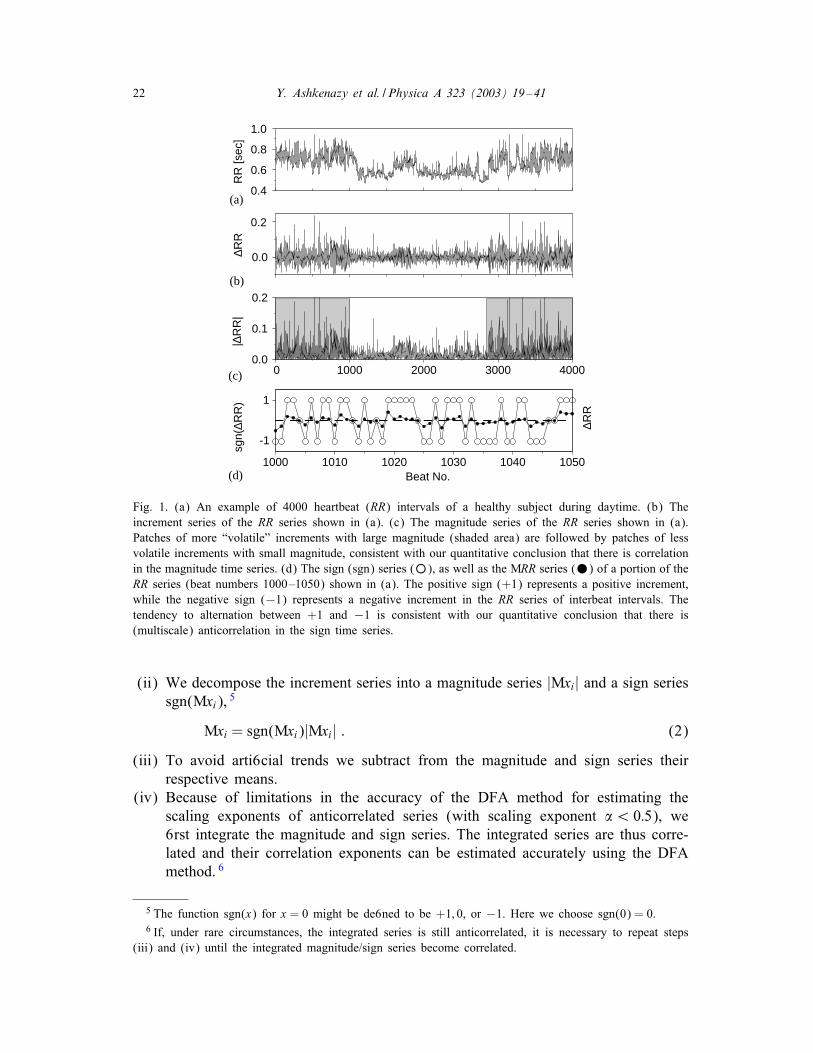
Fig. 1. (a) An example of 4000 heartbeat (RR) intervals of a healthy subject during daytime. (b) The

increment series of the RR series shown in (a). (c) The magnitude series of the RR series shown in (a).

Patches of more “volatile” increments with large magnitude (shaded area) are followed by patches of less

volatile increments with small magnitude, consistent with our quantitative conclusion that there is correlation

in the magnitude time series. (d) The sign (sgn) series (◦), as well as the MRR series (•) of a portion of the

RR series (beat numbers 1000–1050) shown in (a). The positive sign (+1) represents a positive increment,

while the negative sign (−1) represents a negative increment in the RR series of interbeat intervals. The

tendency to alternation between +1 and −1 is consistent with our quantitative conclusion that there is

(multiscale) anticorrelation in the sign time series.

(ii) We decompose the increment series into a magnitude series |Mxi| and a sign series

sgn(Mxi),5

Mxi = sgn(Mxi)|Mxi| : (2)

(iii) To avoid arti6cial trends we subtract from the magnitude and sign series their

respective means.

(iv) Because of limitations in the accuracy of the DFA method for estimating the

scaling exponents of anticorrelated series (with scaling exponent �¡ 0:5), we

6rst integrate the magnitude and sign series. The integrated series are thus corre-

lated and their correlation exponents can be estimated accurately using the DFA

method. 6

5 The function sgn(x) for x = 0 might be de6ned to be +1; 0, or −1. Here we choose sgn(0) = 0.6 If, under rare circumstances, the integrated series is still anticorrelated, it is necessary to repeat steps

(iii) and (iv) until the integrated magnitude/sign series become correlated.


(v) We perform a scaling analysis using second-order DFA on the integrated magni-

tude and sign series. 7

(vi) To obtain the scaling exponents for the magnitude and sign series we calculate the

slope of F(n)=n from a log–log plot. We use the normalized Ductuation function

F(n)=n∼ n�−1 to compensate for the additional integration from step (iv). This

enables us to interpret the scaling results on the level of the increment series

[Mxi ; |Mxi|; sgn(Mxi)] instead of on the level of the integrated series.

As a physiological example, we analyze the heart rate data (Fig. 1) for a group of

18 healthy individuals 8 for which it is known [11] that the heartbeat increment time

series is anticorrelated (Figs. 3a and 4a). We 6nd that the magnitude series exhibits

correlated behavior (Figs. 3b and 4b). The sign series, however, exhibits anticorrelated

behavior for window scales smaller than 100 beats (Figs. 3c and 4c); for scales larger

than 100 beats the sign series gradually becomes uncorrelated.

Correlation in the magnitude series indicates that an increment with large (small)

magnitude is more likely to be followed by an increment with large (small) magnitude.

Anticorrelation in the sign series indicates that a positive increment is more likely to

be followed by a negative increment and vice versa. Thus, our result for the temporal

organization of heartbeat Ductuations suggests that, under healthy conditions, a large

magnitude increment in the positive direction is more likely to be followed by a large

magnitude increment in the negative direction. We 6nd that this empirical “rule” holds

over a broad range of time scales from several beats up to ∼ 100 beats (Fig. 3)

[26,31]. 9

3. Linearity and nonlinearity as re�ected by the magnitude and sign series

Scaling laws that are based on two-point correlations cannot reDect the nonlinearity

of a series (see Appendix A) but, as we will show, the two-point correlations in the

magnitude series do reDect the nonlinearity of the original series. For this purpose,

we generate surrogate data out of a heartbeat interval increment time series using a

technique that preserves the two-point correlations (as reDected by the power spectrum)

and the histogram (but not the nonlinearities [32]). Comparison of the original time

series with the surrogate time series shows that Ductuations with an identical scaling

law can exhibit di8erent correlations for the magnitude series.

7 The 6rst-order DFA eliminates constant trends from the original series (or, equivalently, linear trends

from the integrated series) [5,11]; the second-order DFA removes linear trends, and the nth-order DFA

eliminates polynomial trends of order n − 1.8 MIT-BIH Normal Sinus Rhythm Database and BIDMC Congestive Heart Failure Database available at

http://www.physionet.org/physiobank/database/#ecg.9 Heartbeat increment series were investigated by A. Babloyantz and P. Maurer [31]. These studies di8er

from ours because we investigate, quantitatively, normal heartbeats by evaluating the scaling properties of

the magnitude and sign series. In addition, our calculations are based on window scales larger than six and

up to 1000 heartbeats.


A basic approach to creating surrogate data with the same scaling law as the original

data is to perform a Fourier transform on the time series, preserving the amplitudes

but randomizing the Fourier phases, and then to perform an inverse Fourier transform

to create the surrogate series. This procedure should eliminate nonlinearities stored

in the Fourier phases, preserving only the linear features of the original time series

[33]. However, this does not preserve the probability distribution of the time series

and may lead to an erroneous conclusion regarding the nonlinearity of the underlying

process [27].

A technique which eliminates the nonlinearity of the original data but keeps the

same power spectrum and histogram as the original was suggested in Ref. [32]. The

procedure is iterative and consists of the following steps:

(i) Store a sorted list of the original data {xi} and the power spectrum {Sk} of {xi}.(ii) Begin (l= 0) with a random shuPe {x(l=0)

i } of the data.

(iii) Replace the power spectrum {S(l)k } of {x

(l)i } by {Sk} (keeping the Fourier phases

of {S(l)k }) and then transform back.

(iv) Sort the series obtained from (iii).

(v) Replace the sorted series from (iv) by the sorted {xi} and then return to the

pre-sorting order [i.e., the order of the series obtained from (iii)]; the resulting

series is {x(l+1)i }.

Repeat steps (iii)–(v) until convergence (i.e., until series from consecutive iterations

will be almost the same). 10

We iterate steps (iii)–(v) 100 times to create surrogate data of heartbeat incre-

ment series (Fig. 2); we use 100 iterations to make sure that convergence is achieved.

Nonetheless, in some cases, few iterations may be suQcient for convergence. We apply

the surrogate test to the increment series and not to the original series in part because

the increment series is stationary (i.e., the variance of the series remains 6nite when

increasing the series length to in6nity) and is thus more appropriate for the use of the

surrogate data test. The new surrogate series (Fig. 2a) has almost the same Ductua-

tion function F(n) as the original heartbeat increment series, with a scaling exponent

indicating long-range anticorrelations in the interbeat increment series (Fig. 3a). Our

analysis of the sign time series derived from the surrogate series (Fig. 2c) shows scal-

ing behavior almost identical to the scaling of the sign series derived from the original

data (Fig. 3c). On the other hand, the magnitude time series derived from the surrogate

(linearized) signal (Fig. 2b) exhibits uncorrelated behavior—a signi6cant change from

the strongly correlated behavior observed for the original magnitude series (Fig. 3b).

Thus, the increments in the surrogate series do not follow the empirical “rule” ob-

served for the original heartbeat series, although these increments follow a scaling law

10 Another test for nonlinearity [34] consists of the following steps: (i) create a Gaussian white noise,

(ii) reorder it as the original series, (iii) phase-randomize the series, and (iv) reorder the original series

according to the series from (iii). The surrogate series from (iv) has the same distribution and similar power

spectrum as the original series; however, this procedure does not accurately preserve the low frequencies in

the power spectrum [32] and thus is not applicable for series with long-range correlations.


-1

1

sgn(

∆RR

)

0 1000 2000 3000 40000.0

0.1

0.2|∆

RR

|

1000 1010 1020 1030 1040 1050

Beat No.

0.0

0.2

∆RR

Surrogate Data

∆RR

(a)

(b)

(c)

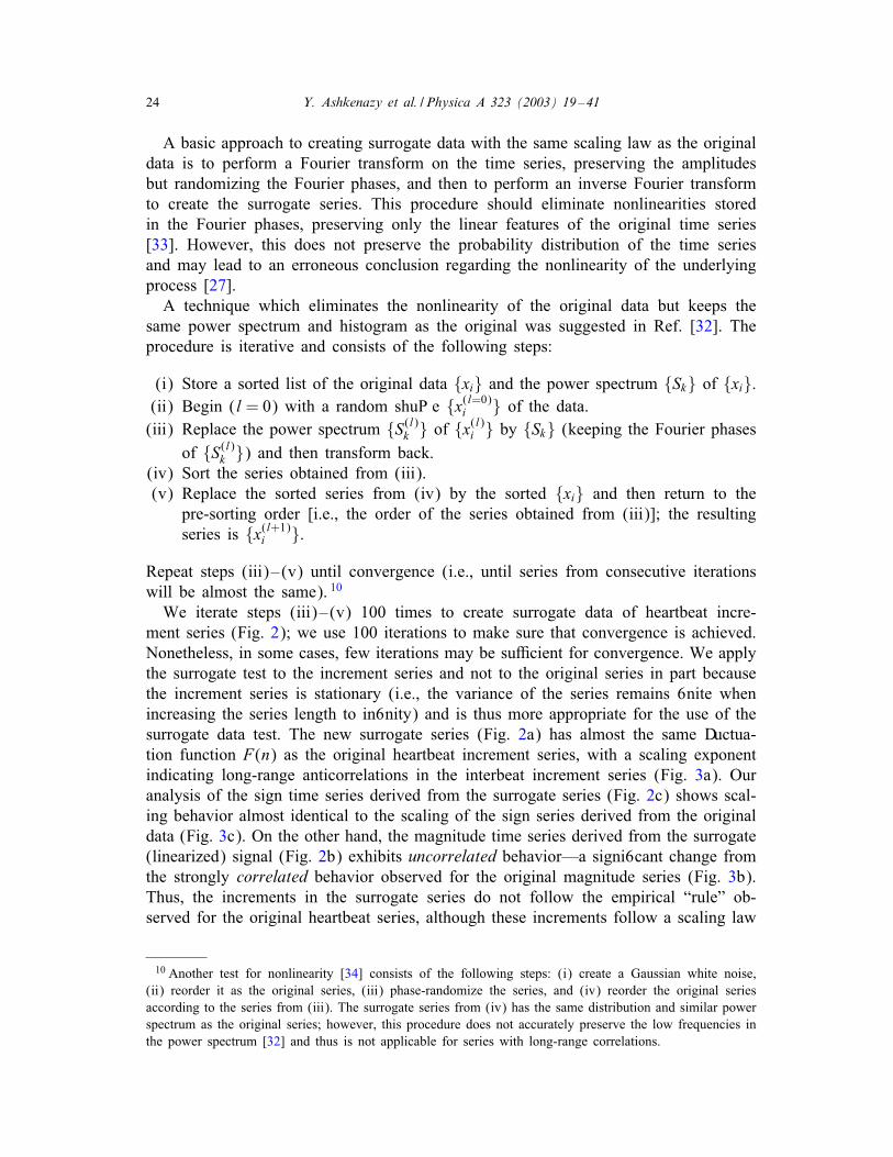
Fig. 2. (a) The surrogate data of the MRR series shown in Fig. 1b. The surrogate increment series has

almost the same two-point correlations and the same probability distribution but random Fourier phases. The

surrogate series is more homogeneous than the original MRR series. (b) The magnitude series decomposed

from the series shown in (a). The magnitude series is homogeneous and does not show the patches of small

and big magnitude values shown in Fig. 1c. This suggests that the “clustering” of the magnitude series is a

measure of nonlinearity. (c) A portion of the sign series of the series shown in (a). The sign series shows

similar alternations as in the original sign series (Fig. 1d).

identical to the original heartbeat increment series. Our results indicate that the magni-

tude series carries information about the nonlinear properties of the original heartbeat

series, while the sign series relates mainly to linear properties.

To further validate these results, we apply the surrogate data test for nonlinearity

to the heartbeat increment series (daily records) of the 18 healthy subjects discussed

above (see footnote 8). For each of the 18 individuals we 6nd that the DFA scaling

exponent of the surrogate data is very close to (although slightly higher than) the

exponent of the original data (Fig. 4a). The small discrepancies between the surrogate

data exponents and the original data exponents might be a result of the 6nite length

and 6nite resolution of the interbeat interval series. The magnitude exponent of the

surrogate data indicates uncorrelated behavior (scaling exponent of � − 1≈ 0:5) for

each of the subjects (Fig. 4b) in contrast to the correlations found in the magnitude

series of the original data. This drastic change from correlated to uncorrelated behavior

for all subjects con6rms our result that the magnitude series carries information about

nonlinear properties of the original data. In Section 5, we show that this type of

nonlinearity is related to multifractality. The sign series exponent of the surrogate data

remains almost unchanged after the surrogate data test (Fig. 4c). Thus, the sign series

seems mainly to reDect the linear properties of the original series.

The di8erence between the exponents before and after the surrogate data test for

nonlinearity may be quanti6ed as follows. If � is the exponent derived from the original


10 100 1000

n

10-1

100

F(n

)/n

10-3

10-2

F(n

)/n

datasurrogate data

10-3

10-2

F(n

)/n

α−1=0.35

(b)

(c)

α−1=0.5

α−1=0.75

α−1=0

(a)

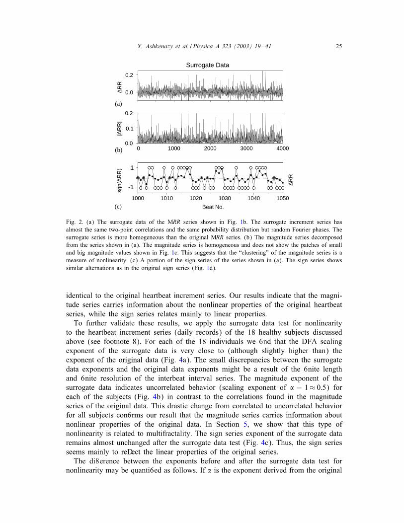
Fig. 3. (a) Root mean square Ductuation, F(n), for ≈ 6 h record (≈ 32 000 data points) for the interbeat

interval RR series ( ) of the healthy subject shown in Fig. 1. Here, n indicates the time scale (in beat

numbers) over which each measure is calculated. The scaling is obtained using second-order detrended

Ductuation analysis, and indicates (since � − 1 = 0) long-range anticorrelations in the heartbeat interval

increment series MRR [11,15]. By construction, the scaling properties of the interval increment series remain

almost unchanged after the surrogate data test (�). (b) The root mean square Ductuation, F(n), of the

integrated magnitude series ( ) indicates long-range correlations in the magnitude series |MRR| (group

average exponent of � − 1 = 0:74± 0:08 where F(n)=n ˙ n�−1). After a surrogate data test applied to the

interbeat interval increment series we 6nd uncorrelated behavior with exponent 0.5 (�). This change in the

scaling suggests that the magnitude series carries information about the nonlinear properties of the original

series since the nonlinear properties are removed by the surrogate test procedure. (c) The root mean square

Ductuation of the integrated sign series ( ) indicates short-range (76 n6 64) anticorrelated behavior in

sgn(MRR) series (group average exponent of � − 1 = 0:32 ± 0:06 where F(n)=n ˙ n�−1). The scaling

properties of the sign series remain unchanged after the surrogate data test (�), which suggests that the sign

series relates to linear properties of the original time series. We note the apparent crossovers at n≈ 20 beats

and n≈ 100 beats. At larger scales (n¿ 64) the sign series loses its speci6city and converges gradually to

� − 1≈ 0:5. Thus, the sign series correlation properties may reveal signi6cant information only for scales

n¡ 100. We note, however, that heartbeat increments derived from the original time series are anticorrelated

up to scales of thousands of heartbeats.

data and S�s; M�s are the average and the standard deviation of the exponents derived

from the surrogate data, then the separation is given by [34]

� = |�− S�s|=M�s : (3)

� measures how many standard deviations the original exponent is separated from

the surrogate data exponent. The larger the � the larger the separation between the

exponents derived from the surrogate data and the exponent derived from the original

data. Thus, larger � values indicate stronger nonlinearity. In Fig. 4d we show the �


values for the magnitude and sign exponents. The � values of the magnitude exponents

are large and thus indicate a signi6cant di8erence between the magnitude exponents of

the original and the surrogate data. On the other hand the � values of the sign exponents

are small, indicating similarity between the sign exponents of the original and surrogate

data. Thus, we conclude that the magnitude series indicates nonlinearity of the original

data. The sign series, on the other hand, relates mainly to the linear properties.

4. The relation between the original, magnitude, and sign series scaling exponents

Recently [26], we investigated the relation between the scaling exponent of the

original series and the scaling exponents of the integrated magnitude series and the

integrated sign series. We generated long-range correlated linear noise with di8erent

scaling exponents ranging from � = 0:5 to 1.5. Then we decomposed the increment

series into a magnitude series and a sign series. Finally, we calculated the scaling

exponents of the integrated magnitude and sign series. At small time scales (n¡ 16),

we found an empirical approximate relation for the scaling exponents,

�sign ≈ 12(�original + �magnitude) : (4)

At larger window scales (n¿ 64), we 6nd that for linear noise with a scaling exponent

�¡ 1:5, the magnitude and sign series of the increments are uncorrelated. In the fol-

lowing we suggest an explanation for these 6ndings. We also show that, for �¿ 1:5 in

the original series, the integrated magnitude series and the integrated sign series have

approximately the same two-point scaling exponent.

We observe uncorrelated behavior for the magnitude series since we use linear noise

(see Section 3 where we 6nd that uncorrelated behavior of the magnitude series reDects

linearity of the original series). In the next section, we show that the magnitude series

is correlated for multifractal nonlinear noise. The sign series exhibits anticorrelated

behavior for small scales and uncorrelated behavior for larger scales, regardless of the

nonlinear properties of the original time series.

At small scales, the sign series coarse grains the increment series and thus preserves

some of its correlation properties. For instance, if the increment series is anticorre-

lated, i.e., a large increment value is followed by a small increment value, the sign

series will also alternate and be anticorrelated. On the other hand, if the incre-

ment series is uncorrelated, the sign series will also perform random behavior and be

uncorrelated.

The power spectrum of long-range anticorrelated series increases in power-law man-

ner. This implies that the amplitudes of low frequencies are much smaller than the

amplitudes of higher frequencies. The crude coarse graining of the increment series by

the sign series mainly approximates the high frequency band (small window scales)

since the majority of the power spectrum lays in this frequency band. However, the sign

series cannot maintain the very small amplitudes of the low frequencies (long-range

anticorrelations) due to the small fraction of the power spectrum at this frequency band.

This may lead to uncorrelated behavior of the sign series for larger window scales.


1 3 5 97 11 13 15 17Subject No.

1.2

1.3

1.4

1.5

1.5

1.7

1.9

Exp

onen

tα

0.8

1

1.2

1.4data

surrogate dataaverage

(b)

(c)

(a)

1 53 7 9 11 13 15 17

Subject No.

0

5

10

15

20

25

30

35

σ fo

r D

FA

Exp

onen

t

magnitude

sign

p<.05

p>.05

(d)


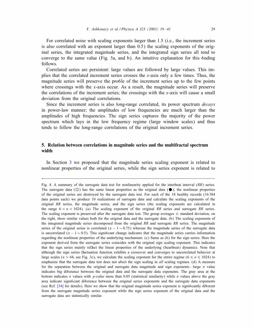
For correlated noise with scaling exponents larger than 1.5 (i.e., the increment series

is also correlated with an exponent larger than 0.5) the scaling exponents of the orig-

inal series, the integrated magnitude series, and the integrated sign series all tend to

converge to the same value (Fig. 5a, and b). An intuitive explanation for this 6nding

follows.

Correlated series are persistent: large values are followed by large values. This im-

plies that the correlated increment series crosses the x-axis only a few times. Thus, the

magnitude series will preserve the pro6le of the increment series up to the few points

where crossings with the x-axis occur. As a result, the magnitude series will preserve

the correlations of the increment series; the crossings with the x-axis will cause a small

deviation from the original correlations.

Since the increment series is also long-range correlated, its power spectrum decays

in power-law manner; the amplitudes of low frequencies are much larger than the

amplitudes of high frequencies. The sign series captures the majority of the power

spectrum which lays in the low frequency regime (large window scales) and thus

tends to follow the long-range correlations of the original increment series.

5. Relation between correlations in magnitude series and the multifractal spectrum

width

In Section 3 we proposed that the magnitude series scaling exponent is related to

nonlinear properties of the original series, while the sign series exponent is related to

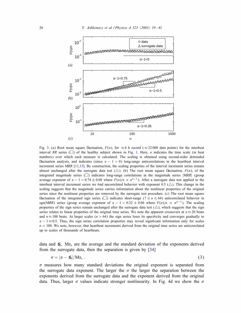
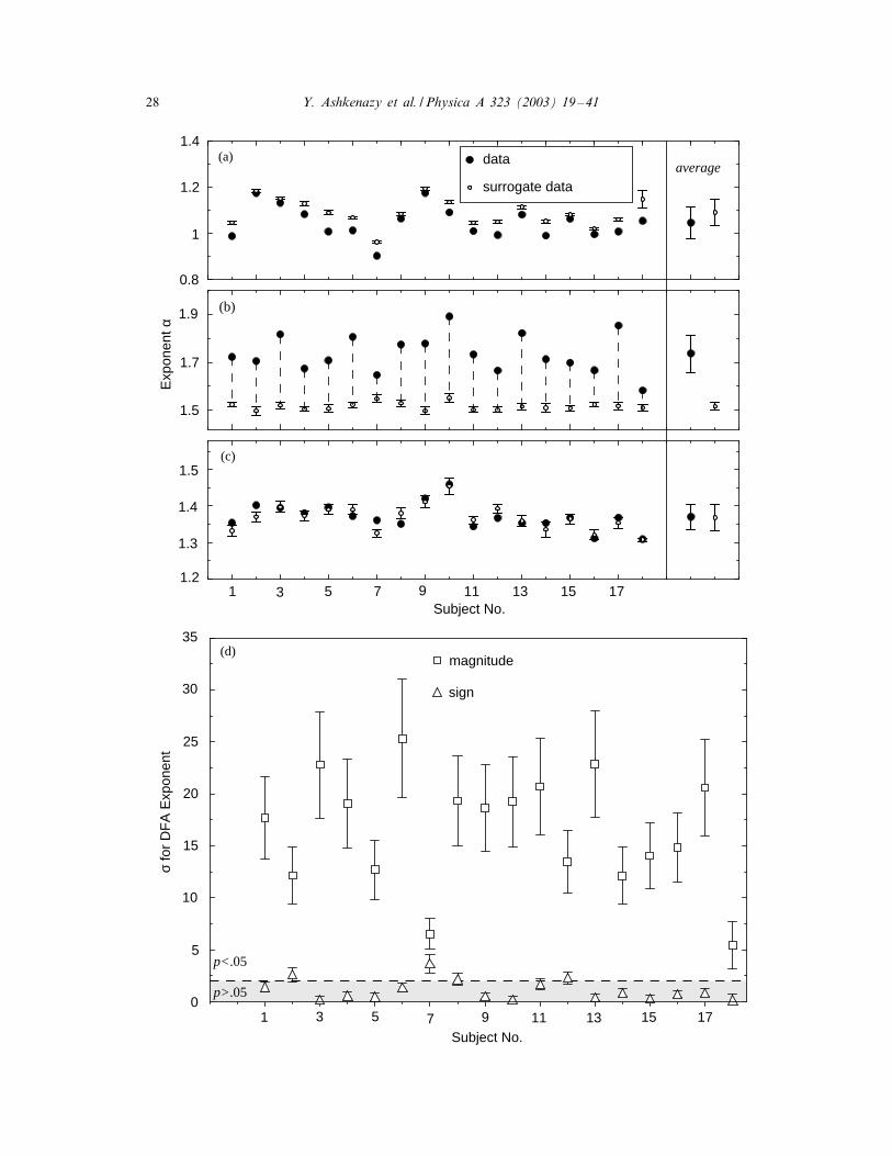
←−−−−−−−−−−−−−−−−−−−−−−−−−−−−−−−−−−−−−−−−−−−−−−−−−−−−−−−−−−−−−−−Fig. 4. A summary of the surrogate data test for nonlinearity applied for the interbeat interval (RR) series.

The surrogate data (◦) has the same linear properties as the original data (•); the nonlinear properties

of the original series are destroyed by the surrogate data test. For each of the 18 healthy records (16 384

data points each) we produce 10 realizations of surrogate data and calculate the scaling exponents of the

original RR series, the magnitude series, and the sign series (the scaling exponents are calculated in

the range 6¡n¡ 1024). (a) The scaling exponent of the original RR series and surrogate RR series.

The scaling exponent is preserved after the surrogate data test. The group averages ± standard deviation, on

the right, show similar values both for the original data and the surrogate data. (b) The scaling exponents of

the integrated magnitude series decomposed from the original RR and surrogate RR series. The magnitude

series of the original series is correlated (� − 1∼ 0:75) whereas the magnitude series of the surrogate data

is uncorrelated (�− 1∼ 0:5). This signi6cant change indicates that the magnitude series carries information

regarding the nonlinear properties of the underlying mechanism. (c) Same as (b) for the sign series. Here the

exponent derived from the surrogate series coincides with the original sign scaling exponent. This indicates

that the sign series mainly reDect the linear properties of the underlying (heartbeat) dynamics. Note that

although the sign series Ductuation function exhibits a crossover and converges to uncorrelated behavior at

large scales (n¿ 64, see Fig. 3c), we calculate the scaling exponent for the entire regime (66 n6 1024) to

emphasize that the surrogate data test does not a8ect the sign scaling in all scaling regimes. (d) A measure

for the separation between the original and surrogate data magnitude and sign exponents—large � value

indicates big di8erence between the original data and the surrogate data exponents. The gray area at the

bottom indicates � values with p-value more than 0.05 (statistical similarity) while � values above the gray

area indicate signi6cant di8erence between the original series exponents and the surrogate data exponents

(see Ref. [34] for details). Here we show that the original magnitude series exponent is signi6cantly di8erent

from the surrogate magnitude series exponent while the sign series exponent of the original data and the

surrogate data are statistically similar.


1.5 1.7 1.9 2.1 2.3 2.5Input Exponent

1.5

1.7

1.9

2.1

2.3

2.5

αlo

ng1.5

1.7

1.9

2.1

2.3

2.5

αsh

ort

αoriginal

αmagnitude

αsign(a)

(b)

Fig. 5. (a) The relation between the scaling exponents of correlated noise, the integrated magnitude series,

and the integrated sign series for the short-range regime (n¡ 16). We generate 10 series of length 32 768

with speci6c correlations (input exponent) and then calculate the scaling exponents of the original series

(•), of the integrated magnitude series ( ), and of the integrated sign series (�); the average ±1 standard

deviation are shown. All three exponents tend to converge to the same value. (b) Same as (a) for the

long-range regime (64¡n¡ 1024). Also in this regime the scaling exponents of the original, magnitude,

and sign series tend to converge to the same value.

linear properties. Here we study what type of nonlinearity is revealed by the magnitude

series correlations.

Linear series with long-range correlations are characterized by linearly dependent

q-order correlation exponents �(q), i.e., the exponents �(q) of di8erent moments q are

linearly dependent,

�(q) = Hq+ �(0) ; (5)

with a single Hurst exponent, 11

H ≡ d�=dq= const : (6)

In this case the series is called monofractal. Long-range correlated nonlinear signals

have a multiple Hurst exponent

h(q) ≡ d�=dq �= const ; (7)

where �(q) depends nonlinearly on q. In this case the series is called multifractal

(MF). The MF spectrum is de6ned by

D(h) = h(q)q− �(q) ; (8)

11 The DFA exponent �=H +1 and the second moment �(2)= 2H + �(0)= 2�− 2+ �(0). For continuous

series �(0) =−1 and thus �(2) = 2� − 3.


where, for a monofractal series, it collapses to a single point,

D(H) =−�(0) : (9)

Here we show the nonlinear measure of the magnitude series scaling exponent to be

related to the MF spectrum D(h).

Indeed, a previous study [14] showed that the healthy heartbeat interval series is

MF and indicated that after Fourier-phase randomization the interbeat interval series

becomes monofractal. Moreover, this study also indicated a loss of multifractality with

disease—heart failure patients have a narrower MF spectrum than healthy individuals.

Comparison of the magnitude series scaling exponent of healthy and heart failure in-

dividuals shows signi6cantly higher exponents for healthy subjects [26]. This result is

additional numerical (although not mathematical) evidence showing that the magnitude

series scaling exponent may be related to the MF spectrum. The change in the mag-

nitude exponent for heart failure subjects is also consistent with a previously reported

loss of nonlinearity with disease [14,35,36].

In order to test the connection between the magnitude scaling exponent and the MF

spectrum, we generate arti6cial noise with built-in MF properties. Then we check how

the magnitude scaling exponent is related to the MF spectrum width.

We use the algorithm proposed in Ref. [37] to generate the arti6cial MF noise. This

algorithm is based on random cascades on wavelet dyadic trees. BrieDy, the random

MF series is built by specifying its discrete wavelet coeQcients cj; k . The coeQcient

cj; k is de6ned recursively as

c0;0 = 1 ;

cj;2k =Wcj−1; k ;

cj;2k+1 =Wcj−1; k (10)

for all j (j¿ 1) and k (06 k ¡ 2j−1), where W is a random variable. Once the

wavelet coeQcients cj; k are constructed, we apply an inverse wavelet transform to gen-

erate MF random series. The MF properties of the series can be determined according

to the distribution of the random variable W .

We consider two di8erent types of probability distributions for the random variable

W : the log-normal distribution and the log-Poisson distribution. For these two examples

the MF properties are known analytically [37]. The MF spectrum D(h) is symmetric

for the log-normal distribution and asymmetric for the log-Poisson distribution. We use

the 10-tap Daubechies discrete wavelet transform [38,39].

5.1. Log-normal W distribution

We consider the case of a log-normal random variable W where ln|W | is nor-

mally distributed and �; �2 are the mean and the variance of ln|W |. For simplicity

we choose �=− 14ln 2. In this case, the scaling exponent of di8erent moments �(q) is


given by

�(q) =− �2

2 ln 2q2 +

q

4− 1 (11)

and the MF spectrum D(h) is

D(h) =− (h− 1=4)2 ln 2

2�2+ 1 : (12)

The MF spectrum width can be found by solving D(h) = 0 and is

hmax − hmin =

( √2�√ln 2

+1

4

)

−(

−√2�√ln 2

+1

4

)

=2√2�√

ln 2: (13)

Thus for � = 0 the series will be monofractal and, for larger � values, will have a

broader MF spectrum (Eq. (13)). It is also clear that for � → 0; D(H = 1=4) = 1

(Eqs. (12), (13)), and for larger values of �, the MF spectrum is symmetric around

D(1=4) = 1 (Fig. 6a, b).

We generate series with di8erent � values ranging from 0 to 0.1 (20 realizations for

each �) and calculate the original, magnitude, and sign scaling exponents (Fig. 6c). We

6nd that indeed the original series exponent has a 6xed value ≈ 1:25; this exponent

is consistent with the Hurst exponent H = 0:25 since the DFA exponent � = H + 1.

The sign series also has a 6xed value ≈ 1:45 (see Ref. [26]). The magnitude series

scaling exponent increases monotonically with � from uncorrelated magnitude series

with scaling exponent �−1≈ 0:5 to strongly correlated magnitude series with exponent

�− 1≈ 1. The magnitude exponent converges to �− 1 = 1.

Since there is a linear relation between � and the MF spectrum width (Eq. (13))

and since the magnitude exponent increases monotonically with �, we suggest that the

magnitude exponent is related to the MF spectrum width.

5.2. Log-Poisson W distribution

In the previous section, we study an example with a symmetric MF spectrum D(h).

Here we show that changes in the magnitude scaling exponent are not a result of

changes in the positive moments only (and especially the fourth moment) but rather

reDect changes of the entire MF spectrum. For this purpose we study an example with

an asymmetric MF spectrum where the exponents for negative moments, h(q¡ 0), are

changed drastically when the MF spectrum width is changed while h(q¿ 0) is less

signi6cantly changed. We tune the parameters in such a way that the fourth moment

�(4) is 6xed and the second moment �(2) is hardly changed.

We consider the case of a log-Poisson random variable W , where � is the mean and

also the variance of Poisson variable P, and ln|W | has the same distribution function

as P ln �+ �; � is an appropriately chosen positive parameter [37]. We choose �=ln 2

and �=−�4 ln 2=4. Under this choice of parameters,

�(q) =−�q + q�4=4 (14)


-10 -5 50 10q

-4

-3

-2

-1

0

1

τ (q

)

0.2 0.4h

0

1

D (

h)

hminhmaxν=0

ν=0.1

ν=0

ν=0.1

0 0.02 0.04 0.06 0.08 0.1

ν

1.2

1.4

1.6

1.8

2

Exp

onen

t

original

magnitude

sign

(a) (b)

(c)

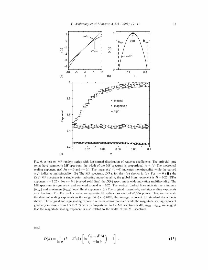
Fig. 6. A test on MF random series with log-normal distribution of wavelet coeQcients. The arti6cial time

series have symmetric MF spectrum; the width of the MF spectrum is proportional to �. (a) The theoretical

scaling exponent �(q) for �=0 and �=0:1. The linear �(q) (�=0) indicates monofractality while the curved

�(q) indicates multifractality. (b) The MF spectrum, D(h), for the �(q) shown in (a). For � = 0 (•) the

D(h) MF spectrum is a single point indicating monofractality; the global Hurst exponent is H = 0:25 (DFA

exponent �=1:25). For �=0:1 (curved solid line) the D(h) spectrum is wide indicating multifractality. The

MF spectrum is symmetric and centered around h = 0:25. The vertical dashed lines indicate the minimum

(hmin) and maximum (hmax) local Hurst exponents. (c) The original, magnitude, and sign scaling exponents

as a function of �. For each � value we generate 20 realizations each of 65 536 points. Then we calculate

the di8erent scaling exponents in the range 646 n6 4096; the average exponent ±1 standard deviation is

shown. The original and sign scaling exponent remains almost constant while the magnitude scaling exponent

gradually increases from 1.5 to 2. Since � is proportional to the MF spectrum width, hmax−hmin , we suggest

that the magnitude scaling exponent is also related to the width of the MF spectrum.

and

D(h) =1

ln �(h− �4=4)

[

ln

(

h− �4=4

−ln �

)

− 1

]

: (15)


Thus, the fourth moment �(4) is independent of �

�(4) = 0 (16)

and the width of the MF spectrum depends on �

hmax − hmin = (�4=4− e ln �)− (�4=4) =−e ln � : (17)

For � = 1 the MF spectrum collapses and becomes a single point (monofractal) with

Hurst exponent H=1=4 and D(1=4)=1. For decreasing or increasing � the MF spectrum

becomes wider. Here we change the MF spectrum width by decreasing �; the major

change in the MF spectrum occurs for negative moments q¡ 0 (Fig. 7a and b).

In Fig. 7c we show the scaling exponents of the original, magnitude, and sign series

for di8erent values of �. We 6nd that the original and sign series exponents hardly

change with �, while the magnitude exponent increases monotonically. This increase

suggests that the magnitude scaling exponent is related to the MF spectrum width (see

also Fig. 6).

We summarize the results of the log-normal and the log-Poisson examples in

Fig. 7d—the magnitude scaling exponent is plotted versus the width of the MF spec-

trum [Eqs. (13), (17)]. Surprisingly, these two examples collapse to the same curve.

This collapse suggests a possible one-to-one relation 12 between the magnitude scaling

exponent and the MF spectrum width. 13

The relation between the magnitude scaling exponent and the MF spectrum width

is consistent with a recent study of Bacry et al. [40]. It was shown there that it is

possible to generate an MF series xi with Gaussian random variables !l, !l,

xi =

i∑

l=1

Mxl =

i∑

l=1

!le!l : (18)

For correlated !l the series xi is MF, while for uncorrelated !l it is monofractal.

Stronger correlations in !l yields broader MF spectrum. The magnitude series |Mxl|is equivalent to the positive numbers e!l while the sign series may be represented by

the real numbers !l. Thus, correlations in |Mxl| may be related to correlations in e!l

and both may be related to the MF spectrum width. We note that this comparison

is qualitative since the sign series is a binary series (+1 or −1) while the !l is a

continuously valued Gaussian random variable.

The results described in this section may be important from a practical point of

view since the calculation of the MF spectrum from a time series involves advanced

12 We de6ne a one-to-one relation as follows: let y = f(x), then if x is a single-valued function of y and

y is a single-valued function of x then x and y are one-to-one related.13 We also performed the same procedure (as in Figs. 6, 7) for a deterministic multifractal object, namely

the generalized devil’s staircase [41]. Also here we 6nd that magnitude exponent increases monotonically

with the multifractal spectrum width. However, for very small multifractal width the magnitude exponent

was ∼ 1 and then increased sharply to the behavior shown in Fig. 7d; this behavior might be related to the

deterministic nature of this multifractal object.


-10 -5 0 5 10q

-4

-3

-2

-1

0

1

τ (q

)

0.2 0.4h

0

1

D (

h)

hmin hmaxδ=1

δ=0.9

δ=1

δ=0.9

0 0.02 0.04 0.06 0.08 0.1–ln (δ)

1.2

1.4

1.6

1.8

2

Exp

onen

t

originalmagnitudesign

0 0.1 0.2 0.3 0.4Multifractal width [hmax –hmin ]

1.5

1.6

1.7

1.8

1.9

2

Mag

nitu

de E

xpon

ent

lognormal dist.logpoisson dist.

(a) (b)

(c) (d)

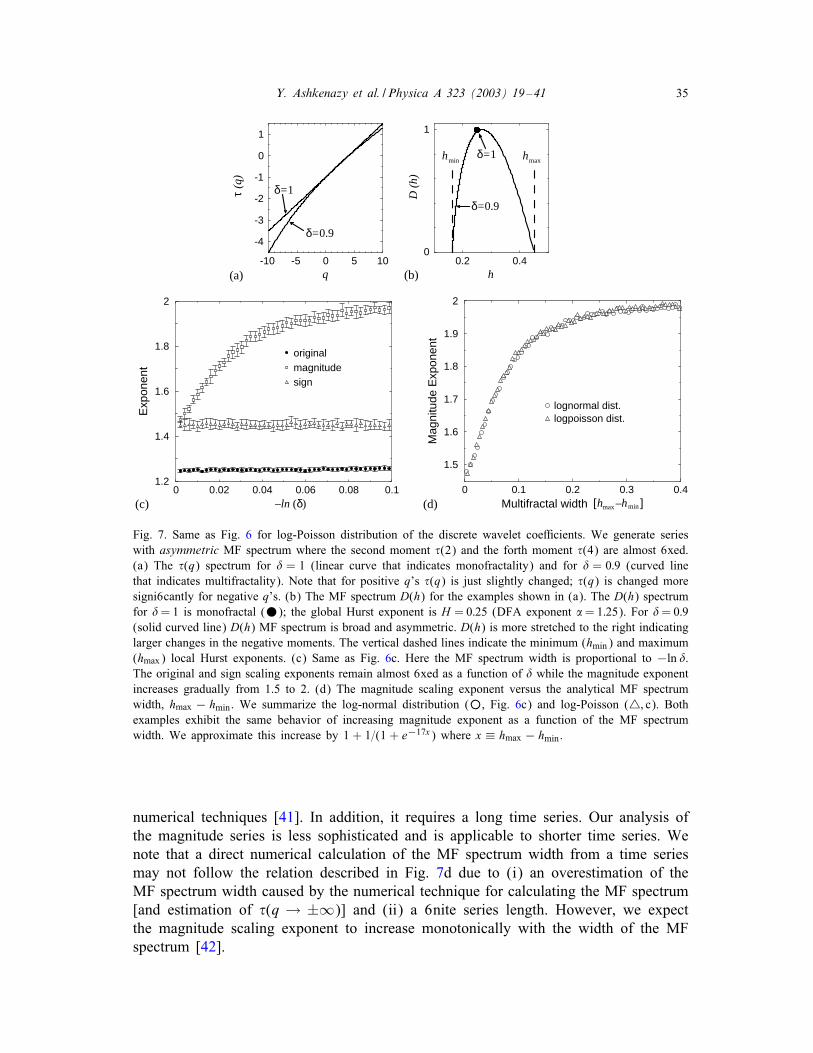
Fig. 7. Same as Fig. 6 for log-Poisson distribution of the discrete wavelet coeQcients. We generate series

with asymmetric MF spectrum where the second moment �(2) and the forth moment �(4) are almost 6xed.

(a) The �(q) spectrum for � = 1 (linear curve that indicates monofractality) and for � = 0:9 (curved line

that indicates multifractality). Note that for positive q’s �(q) is just slightly changed; �(q) is changed more

signi6cantly for negative q’s. (b) The MF spectrum D(h) for the examples shown in (a). The D(h) spectrum

for �= 1 is monofractal (•); the global Hurst exponent is H = 0:25 (DFA exponent �= 1:25). For �= 0:9

(solid curved line) D(h) MF spectrum is broad and asymmetric. D(h) is more stretched to the right indicating

larger changes in the negative moments. The vertical dashed lines indicate the minimum (hmin) and maximum

(hmax) local Hurst exponents. (c) Same as Fig. 6c. Here the MF spectrum width is proportional to −ln �.

The original and sign scaling exponents remain almost 6xed as a function of � while the magnitude exponent

increases gradually from 1.5 to 2. (d) The magnitude scaling exponent versus the analytical MF spectrum

width, hmax − hmin . We summarize the log-normal distribution (◦, Fig. 6c) and log-Poisson (�; c). Both

examples exhibit the same behavior of increasing magnitude exponent as a function of the MF spectrum

width. We approximate this increase by 1 + 1=(1 + e−17x) where x ≡ hmax − hmin .

numerical techniques [41]. In addition, it requires a long time series. Our analysis of

the magnitude series is less sophisticated and is applicable to shorter time series. We

note that a direct numerical calculation of the MF spectrum width from a time series

may not follow the relation described in Fig. 7d due to (i) an overestimation of the

MF spectrum width caused by the numerical technique for calculating the MF spectrum

[and estimation of �(q → ±∞)] and (ii) a 6nite series length. However, we expect

the magnitude scaling exponent to increase monotonically with the width of the MF

spectrum [42].


6. Diagnostic utility of magnitude and sign scaling exponents on heartbeat interval

series

In a previous study, we showed that statistics obtained from the magnitude and sign

series of heartbeat increments can be used to separate healthy subjects from those with

heart failure [26]. In that work, heartbeat interval records of up to 6 h; ≈ 30; 000

points, were analyzed. Here, we show that an even shorter time series—of the order of

2000 points (∼ 1=2 h)—can yield a signi6cant separation between healthy individuals

and those with heart failure.

Our analysis is based on 24 h Holter recordings from 18 healthy individuals (Fig. 4)

and from 12 individuals with congestive heart failure (see footnote 8). We subdivide

each record to segments of 1024 data points and use the DFA method to calculate

the Ductuation function F(n). We choose the scale n = 16 to be the crossover point

since it separates between a short-range regime (6¡n¡ 16) with exponent �1, and

an intermediate-range regime (166 n6 64) with exponent �2. We perform our scaling

analysis for the original series, as well as the magnitude and sign sub-series. For each

time segment we show the 1=2 h average scaling exponent of the healthy and heart

failure groups (Fig. 8).

The short-range exponent �1 of the original RR series (Fig. 8a) shows good sepa-

ration between the healthy and heart failure groups [43]. During nighttime the healthy

exponent drops towards the heart failure exponent. This might be related to the lower

scaling exponent of interbeat interval series of healthy subjects during light and deep

sleep episodes [15]. In addition, the heart failure group shows an apparent slow

oscillatory-like behavior of two cycles per 24 h period. The intermediate exponent

does not show a clear separation between the two groups.

The short and intermediate-range magnitude series exponents also distinguish be-

tween the interbeat patterns of healthy and unhealthy hearts (Fig. 8b). For short range,

the scaling exponent for the heart failure group is systematically larger than for the

healthy group while for the intermediate-range exponent we observe the opposite. Thus,

there is a crossover behavior in the magnitude exponent both for healthy individuals

and those with heart failure; this crossover might be related to the crossover of the

interbeat intervals series [11] since the original, magnitude, and sign exponents depend

on one another at small scales (Section 4). At larger scales (n¿ 64, not shown) the

separation between healthy and unhealthy hearts is signi6cant and might be related to

the decrease of nonlinearity with disease [26].

The behavior of the sign series is similar to that of the original heartbeat increment

series (Fig. 8c). The short-range exponent �1 is larger for healthy subjects. In addition,

the intermediate-range exponent separates between healthy individuals and those with

heart failure; the exponent is smaller for the healthy. At night, the healthy tend to

converge toward the heart failure—these changes might be related to the changes in

the sign series during the di8erent sleep stages [44]. We also observe here an apparent

oscillatory-like behavior of two cycles per 24-h period.

In summary, we show that, in addition to the original RR series, the magnitude and

sign sub-series may help to distinguish between the healthy group and the heart failure

group. We also show that a short time series of order of 2000 points (∼ 1=2 h) may


8 12 16 20 24 4 8t – time [hour]

0.5

1.0

1.5

2.0

α 2

Healthy

0.50.91.31.7

α 1

CHF

average

(a)

p<10 -27

p<10-3

8 12 16 20 24 4 8

t – time [hour]

1.2

1.4

1.6

1.8

α 2

1.2

1.4

1.6

1.8

α 1

average

(b)

p<10-15

p<10-11

8 12 16 20 24 4 8

t –time [hour]

1.0

1.2

1.4

1.6

α 2

0.6

1.0

1.4

1.8α 1

average

(c)

p<10-18

p<10-9

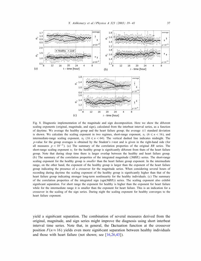
Fig. 8. Diagnostic implementation of the magnitude and sign decomposition. Here we show the di8erent

scaling exponents (original, magnitude, and sign), calculated from the interbeat interval series, as a function

of daytime. We average the healthy group and the heart failure group; the average ±1 standard deviation

is shown. We calculate the scaling exponent in two regimes, short-range exponent, �1 (66 n¡ 16), and

intermediate-range scaling exponent, �2 (166 n¡ 64). The vertical dashed line indicates midnight. The

p-value for the group averages is obtained by the Student’s t-test and is given in the right-hand side (for

all measures p¡ 10−3). (a) The summary of the correlation properties of the original RR series. The

short-range scaling exponent �1 for the healthy group is signi6cantly di8erent from thats of the heart failure

group. Note that during sleep time there is larger overlap between the healthy and heart failure group.

(b) The summary of the correlation properties of the integrated magnitude (|MRR|) series. The short-range

scaling exponent for the healthy group is smaller than the heart failure group exponent. In the intermediate

range, on the other hand, the exponent of the healthy group is larger than the exponent of the heart failure

group indicating the presence of a crossover for the magnitude series. When considering several hours of

recording during daytime the scaling exponent of the healthy group is signi6cantly higher than that of the

heart failure group indicating stronger long-term nonlinearity for the healthy individuals. (c) The summary

of the correlation properties of the integrated sign (sgn(MRR)) series. The scaling exponent also exhibit

signi6cant separation. For short range the exponent for healthy is higher than the exponent for heart failure

while for the intermediate range it is smaller than the exponent for heart failure. This is an indication for a

crossover in the scaling of the sign series. During night the scaling exponent for healthy converges to the

heart failure exponent.

yield a signi6cant separation. The combination of several measures derived from the

original, magnitude, and sign series might improve the diagnosis using short interbeat

interval time series. Note that, in general, the Ductuation function at the crossover

position F(n≈ 16) yields even more signi6cant separation between healthy individuals

and those with heart failure (not shown; see [16,26,43]).


7. Summary

We conclude that series with identical correlation properties can have completely

di8erent time ordering which can be characterized by di8erent scaling exponents for the

magnitude and sign series. The magnitude series reDects the way the series increments

are clustered (volatility [25]) while the sign reDects the way they alternate. Moreover,

we show that the magnitude series carries information regarding nonlinear properties of

the original series while the sign series carries information regarding linear properties

of the original series. The nonlinearity, as reDected by the magnitude series scaling

exponent, is related to the width of the multifractal spectrum of the original series.

Application of the magnitude and sign decomposition on heartbeat increment series

helps us to suggest a dynamical rule of healthy heartbeat increments—a big heartbeat

increment in the positive direction is likely to be followed by a big increment in the

negative direction. Moreover, the magnitude and sign scaling exponents may be used

for diagnostic purposes. Because information obtained by decomposing the original

heartbeat time series into magnitude and sign time series likely reDects aspects of

neuroautonomic regulation, this type of analysis may help address the challenge of

developing realistic models of heart rate control in health and disease.

Acknowledgements

Partial support was provided by the NIH/National Center for Research Resources

(P41 RR13622), the Israel-USA Binational Science Foundation, and the German Aca-

demic Exchange Service (DAAD). We thank L.A.N. Amaral, D. Baker, S.V. Buldyrev,

A. Bunde, J.M. Hausdor8, R. Karasik, J.W. Kantelhardt, G. Paul, Y. Yamamoto, and

especially to A.L. Goldberger for helpful discussions.

Appendix A. Nonlinearity and multifractality

In this appendix we de6ne the linearity and nonlinearity of a time series. We also

review the relation between the multifractality of a time series and its nonlinearity.

Following Refs. [27,32] we de6ne a time series to be linear if it is possible to repro-

duce its statistical properties from the power spectrum and the probability distribution

alone, regardless of the Fourier phases [27]. This de6nition includes (i) autoregression

processes

xn =

M∑

i=1

aixn−i +

L∑

i=0

bi*n−i ; (A.1)

where * is Gaussian white noise and (ii) fractional Brownian motion [45]; the output,

xn, of these processes may undergo monotonic nonlinear transformations

sn = s(xn) (A.2)


and still be linear [27]. Processes which are not linear are de6ned as nonlinear. It

is possible to destroy the nonlinearity of a time series by basically randomizing its

Fourier phases (see Refs. [27,32] and Section 3).

A nonlinearity (linearity) of a time series is related to its multifractality. The de6-

nition of multifractality is based on the partition function Zq(l) of a time series sn and

may be de6ned as [46]

Zq(l) = 〈|sn+l − sn|q〉 ; (A.3)

where 〈·〉 stands for expectation value. In some cases Zq(l) obeys scaling laws

Zq(l)∼ l,q : (A.4)

If the exponents ,q are linearly dependent on q, the series sn is monofractal; if they

are not, sn is multifractal. (Note that in the present study we use a more advanced

method to calculate multifractality that can accurately estimate the exponents of nega-

tive moments q¡ 0 [41].)

The two-point correlation function of an increment time series Msn is de6ned as

A(l) = 〈MsnMsn+l〉 : (A.5)

For long-range correlated stationary Gaussian time series

A(l)∼ l−� ; (A.6)

where 0¡�¡ 1. In this case, the exponent � is related to the DFA exponent � of a

Msn series by [47,48]

Z2(l)∼〈snsn+l〉∼ l2−� = l2� : (A.7)

In addition, these exponents are related to the power spectrum exponent, ., of the

increment series Msn

S(f)∼ 1=f. (A.8)

by

. = 1− �= 2�− 1 : (A.9)

Thus, the second moment only depends on the power spectrum and is independent of

the Fourier phases

,2 = 2�= . + 1 : (A.10)

For monofractal series [41,49],

,q = �q=. + 1

2q : (A.11)

Thus, the MF spectrum of monofractal series is independent of the Fourier phases. This

implies that (i) a long-range correlated series that has uncorrelated Fourier phases is

monofractal and (ii) after randomizing the Fourier phases of an MF series it becomes

monofractal [14].

In summary, monofractal series are linear since their statistical properties depend

only on the power spectrum (two-point correlations) and the probability distribution.


On the other hand, MF series are nonlinear since their higher moments are not solely

dependent on the probability distribution and the power spectrum, but also related to

the Fourier phases.

References

[1] M.F. Shlesinger, Ann. NY Acad. Sci. 504 (1987) 214.

[2] T. Vicsek, Fractal Growth Phenomenon, 2nd Edition, World Scienti6c, Singapore, 1993.

[3] H. Takayasu, Fractals in the Physical Sciences, Manchester University Press, Manchester, UK, 1997.

[4] C.-K. Peng, S.V. Buldyrev, A.L. Goldberger, S. Havlin, F. Sciortino, M. Simons, H.E. Stanley, Nature

356 (1992) 168.

[5] C.-K. Peng, S.V. Buldyrev, S. Havlin, M. Simons, H.E. Stanley, A.L. Goldberger, Phys. Rev. E 49

(1994) 1685.

[6] S.V. Buldyrev, A.L. Goldberger, S. Havlin, R.N. Mantegna, M.E. Matsa, C.-K. Peng, M. Simons,

H.E. Stanley, Phys. Rev. E 51 (1995) 5084.

[7] A. Arneodo, E. Bacry, P.V. Graves, J.F. Muzy, Phys. Rev. Lett. 74 (1995) 3293.

[8] B. Audit, C. Thermes, C. Vaillant, Y. d’Aubenton-Carafa, J.F. Muzy, A. Arneodo, Phys. Rev. Lett. 86

(2001) 2471.

[9] M. Kobayashi, T. Musha, IEEE Trans. Biomed. Eng. 29 (1982) 456.

[10] C.-K. Peng, J. Mietus, J.M. Hausdor8, S. Havlin, H.E. Stanley, A.L. Goldberger, Phys. Rev. Lett. 70

(1993) 1343.

[11] C.-K. Peng, S. Havlin, H.E. Stanley, A.L. Goldberger, Chaos 5 (1995) 82;

C.-K. Peng, S. Havlin, J.M. Hausdor8, J.E. Mietus, H.E. Stanley, A.L. Goldberger, J. Electrocardiol.

28 (1995) 59.

[12] K.K.L. Ho, G.B. Moody, C.-K. Peng, J.E. Mietus, M.G. Larson, D. Levy, A.L. Goldberger, Circulation

96 (1997) 842.

[13] P.-A. Absil, R. Sepulchre, A. Bilge, P. Gerard, Physica A 272 (1999) 235.

[14] P.Ch. Ivanov, L.A.N. Amaral, A.L. Goldberger, S. Havlin, M.G. Rosenblum, Z.R. Struzik, H.E. Stanley,

Nature 399 (1999) 461.

[15] A. Bunde, S. Havlin, J.W. Kantelhardt, T. Penzel, J.H. Peter, K. Voigt, Phys. Rev. Lett. 85 (2000)

3736.

[16] Y. Ashkenazy, M. Lewkowicz, J. Levitan, S. Havlin, K. Saermark, H. Moelgaard, P.E. Bloch Thomsen,

M. Moller, U. Hintze, H.V. Huikuri, Europhys. Lett. 53 (2001) 709.

[17] S. Blesic, S. Milosevic, D. Stratimirovic, M. Ljubisavljevic, Physica A 268 (1999) 275.

[18] J.M. Hausdor8, C.-K. Peng, Z. Ladin, J.Y. Wei, A.L. Goldberger, J. Appl. Physiol. 78 (1995) 349;

J.M. Hausdor8, S.L. Mitchell, R. Firtion, C.-K. Peng, M.E. Cudkowicz, J.Y. Wei, A.L. Goldberger,

J. Appl. Physiol. 82 (1997) 262.

[19] J.D. Pelletier, J. Climate 10 (1997) 1331.

[20] E. Koscielny-Bunde, A. Bunde, S. Havlin, H.E. Roman, Y. Goldreich, H.-J. Schellnhuber, Phys. Rev.

Lett. 81 (1998) 729.

[21] P. Talkner, R.O. Weber, Phys. Rev. E 62 (2000) 150.

[22] K. Ivanova, M. Ausloos, Physica A 274 (1999) 349.

[23] K. Ivanova, M. Ausloos, E.E. Clothiaux, T.P. Ackerman, Europhys. Lett. 52 (2000) 40.

[24] R.N. Mantegna, H.E. Stanley, Nature 376 (1995) 46.

[25] Y. Liu, P. Gopikrishnan, P. Cizeau, M. Meyer, C.-K. Peng, H.E. Stanley, Phys. Rev. E 60 (1999) 1390.

[26] Y. Ashkenazy, P.Ch. Ivanov, S. Havlin, C.-K. Peng, A.L. Goldberger, H.E. Stanley, Phys. Rev. Lett.

86 (2001) 1900.

[27] T. Schreiber, A. Schmitz, Physica D 142 (2000) 346.

[28] J.W. Kantelhardt, E. Koscielny-Bunde, H.H.A. Rego, S. Havlin, A. Bunde, Physica A 295 (2001) 441.

[29] K. Hu, P.Ch. Ivanov, Z. Chen, P. Carpena, H.E. Stanley, Phys. Rev. E 64 (2001) 011 114;

Z. Chen, P.Ch. Ivanov, K. Hu, H.E. Stanley, Phys. Rev. E 65 (2002) 041 107.

[30] Y. Ashkenazy, P.Ch. Ivanov, S. Havlin, C.-K. Peng, Y. Yamamoto, A.L. Goldberger, H.E. Stanley,

Comput. Cardiology 27 (2000) 139.


[31] A. Babloyantz, P. Maurer, Phys. Lett. A 221 (1996) 43;

P. Maurer, H.-D. Wang, A. Babloyantz, Phys. Rev. E 56 (1997) 1188.

[32] T. Schreiber, A. Schmitz, Phys. Rev. Lett. 77 (1996) 635.

[33] P.F. Panter, Modulation, Noise, and Spectral Analysis Applied to Information Transmission,

McGraw-Hill, New York, NY, 1965.

[34] J. Theiler, S. Eubank, A. Longtin, B. Galdrikian, J.D. Farmer, Physica D 58 (1992) 77.

[35] J. Kurths, A. Voss, P. Saparin, A. Witt, H.J. Kleiner, N. Wessel, Chaos 5 (1995) 88;

A. Voss, N. Wessel, H.J. Kleiner, J. Kurths, R. Dietz, Nonlinear Anal.-Theor. 30 (1997) 935.

[36] G. Sugihara, W. Allan, D. Sobel, K.D. Allan, Proc. Natl. Acad. Sci. USA 93 (1996) 2608.

[37] A. Arneodo, E. Bacry, J.F. Muzy, J. Math. Phys. 39 (1998) 4142;

A. Arneodo, S. Manneville, J.F. Muzy, Euro. Phys. J. B 1 (1998) 129.

[38] I. Daubechies, Ten Lectures on Wavelets, SIAM, Philadelphia, PA, 1992.

[39] W.H. Press, S.A. Teukolsky, W.T. Vetterling, B.P. Flannery, Numerical Recipes in C, 2nd Edition,

Cambridge University Press, Cambridge, MA, 1995.

[40] E. Bacry, J. Delour, J.F. Muzy, Phys. Rev. E 64 (2001) 026 103.

[41] J.F. Muzy, E. Bacry, A. Arneodo, Int. J. Bifurcat. Chaos 4 (1994) 245.

[42] Y. Ashkenazy, J.M. Hausdor8, P.Ch. Ivanov, H.E. Stanley, Physica A 316 (2002) 662.

[43] Y. Ashkenazy, M. Lewkowicz, J. Levitan, S. Havlin, K. Saermark, H. Moelgaard, P.E.B. Thomsen,

Fractals 7 (1999) 85.

[44] J.W. Kantelhardt, Y. Ashkenazy, P.Ch. Ivanov, A. Bunde, S. Havlin, T. Penzel, J.-H. Peter, H.E. Stanley,

Phys. Rev. E 65 (2002) 051 908.

[45] B.B. Mandelbrot, J.W. Van Ness, SIAM Rev. 10 (1968) 422–437.

[46] A.L. Barabasi, T. Vicsek, Phys. Rev. A 44 (1991) 2730.

[47] M.S. Taqqu, V. Teverovsky, W. Willinger, Fractals 3 (1995) 785.

[48] H.A. Makse, S. Havlin, M. Schwartz, H.E. Stanley, Phys. Rev. E 53 (1996) 5445.

[49] J.F. Muzy, E. Bacry, A. Arneodo, Phys. Rev. E 47 (1993) 875.

Magnitude and Sign Scaling in Power-Law Correlated Time Series

Documents

Transcript of Magnitude and Sign Scaling in Power-Law Correlated Time Series