Hydrological and 1 D Hydrodynamic Modelling in Manali Sub ...
91
Hydrological and 1 D Hydrodynamic Modelling in Manali Sub-Basin of Beas River, Himachal Pradesh, India Dilip Kumar Maity January, 2009
-
Upload
khangminh22 -
Category
Documents
-
view
3 -
download
0
Transcript of Hydrological and 1 D Hydrodynamic Modelling in Manali Sub ...
Hydrological and 1 D Hydrodynamic Modelling in Manali Sub-Basin of Beas River, Himachal Pradesh, India
Dilip Kumar Maity January, 2009
Hydrological and 1 D Hydrodynamic Modelling in Manali Sub-Basin of Beas River, Himachal Pradesh, India.
by
Dilip Kumar Maity
Thesis submitted to the International Institute for Geo-information Science and Earth Observation in partial fulfilment of the requirements for the degree of Master of Science in Geo-information Science and Earth Observation, Specialisation: (Geo-Hazards) Thesis Assessment Board: Chairman : Dr. Ir. Chris M. M. Mannaerts (ITC, The Netherlands) External Examiner : Dr. D. S. Arya (IIT, Roorkee, India) ITC Member : Ir. Gabriel Norberto Parodi (ITC) IIRS Member : Dr. V. Hari Prasad (In-Charge, WRD) IIRS Member : Ir. Praveen K. Thakur Thesis Supervisors: Ir. Praveen K. Thakur (IIRS) Ir. Gabriel Norberto Parodi (ITC)
INTERNATIONAL INSTITUTE FOR GEO-INFORMATION SCIENCE AND EARTH OBSERVATION ENSCHEDE, THE NETHERLANDS
& INDIAN INSTITUTE OF REMOTE SENSING, NATIONAL REMOTE SENSING CENTRE (NRSC),
DEPARTMENT OF SPACE, DEHRADUN, INDIA

I certify that I might have conferred with others in preparing for this assignment, and drawn upon a range of sources in this work, the content of this thesis work is my original work. Signed…………………………………
Disclaimer This document describes work undertaken as part of a programme of study at the International Institute for Geo-information Science and Earth Observation. All views and opinions expressed therein remain the sole responsibility of the author, and do not necessarily represent those of the institute.

“Only a well-designed channel performs its function best. A blind inert force necessitates intelligent control.”
MAHABHARATA
Dedicated To: My Beloved Grandfather
Who Lead Me To The Glory Of Education

i
Abstract This study introduces about the parameterization of hydrologic and hydraulic modelling for flood inundated area mapping. HEC-HMS, a semi-distributed hydrological model is used for hydrographs generation at predetermined locations and these hydrographs are used as upstream boundary input in MIKE-11 hydraulic model. Palchan to Manali stretch in Beas Sub-basin is used for hydraulic simulation. The hydrological modelling is done in Manali sub-basin. Bahang SASE and Dhundi, two meteorological stations are used as point locations for temperature and rainfall time series data in HEC-HMS model. Rainfall and temperature are used in daily basis from May to October for 1995, 1999 and 2000. Temperature index (TI) is used for snowmelt water contribution in this high altitude region. Land use and land cover (LULC) map prepared from Landsat ETM+ (30m) is used for Curve Number (CN) generation for hydrological modelling. The other parameters for HEC-HMS are collected and prepared from secondary source with the help of literatures. The hydrological model indicates that the Curve Number (CN) has most influence into the total discharge and the model is validated with about 83% accuracy. Both the hydrological and hydraulic models are validated with Bhakra Beas Management Board observed data at Manali outlet. Due to the lower resolution of digital elevation models (DEMs), these could not represent the channel cross section properly and so these are not used in hydraulic modelling in this highly rugged area and only field surveyed cross-sections (31) are used in Mike-11. The Manning’s ‘N’ values for roughness are prepared from field observation. The output hydrographs from HEC-HMS are used as upstream boundary input in MIKE 11. MIKE 11 is successfully calibrated and validated for the unsteady simulation with 86% accuracy. The simulated discharge is much influenced by bed slope and channel conveyance. The difference in water spread area extent in different years with varying rainfall and discharge is clearly observed. KEYWORDS: hydrological and hydraulic modelling, cross-sections, HEC-HMS, MIKE 11, sensitivity analysis, flood inundation mapping.
ii
Acknowledgements The achievement of this paper has come through the overwhelming help that came from many people and sources. I like to express my sincere gratitude to all the people who encouraged me to complete the research work directly or indirectly. I take the opportunity to thank Indian Institute of Remote Sensing (IIRS), Department of space, Government of India and International Institute of Geo-information Science and Earth Observation (ITC), Enschede, The Netherlands for their collaborative MSc. Programme. I would like to express my deep regards to Dr. V. K. Dadhwal, Dean IIRS, Dehradun for permitting me to carry out this research work and for many valuable discussions during the research period. I am thankful to Dr. V. Hariprasad, Programme Coordinator (IIRS), who introduced me to the concept of Disaster, Risk management and other aspects of the research in this field through his teaching. I am also indebted to him for his kind guidance and support during the research work and for providing facilities to carry out the research in IIRS. I am also thankful to Ir. I. C. Das, course coordinator, MSc. Course at IIRS and Dr. Michel Damen, programme coordinator, MSc. Course at ITC. I express my sincere thanks to Ir. Praveen Kumar Thakur, Scientist/Engineer SD, Water Resource Division (WRD), my IIRS supervisor, whose valuable suggestions, serious guidance and assistance leads to the completion of the research work. I am also thankful to Ir. Gabriel Norberto Parodi, Engineer, Water Resource Division, my supervisor at ITC, who inspired me to do this research work with his continuous support and technical guidance. I take the opportunity to thank to my IIRS supervisor for providing the initial idea about the research and guiding me during this phase. I would like to express my thanks to the faculty members of IIRS and ITC who enriched my knowledge by their teaching and guidance during the course directly or indirectly. I gratefully acknowledge the librarians and administrative staffs of IIRS and ITC for their kind help during this MSc course. My special thanks go to Ir. Nitya Nanda Ray, Chief Engineer of Central Water Commission, Dehradun for his useful help regarding MIKE 11 user interface and technical advice at the valuable stage of this research. I wish to convey my thanks to all my previous teachers, seniors, mates and friends at IIRS and Calcutta who supported me a lot during this course. Lastly, I would like to express my heedful gratitude to my parents and family members for their ever support for their loving son in all respect.

iii
Table of contents
1. Introduction ....................................................................................................................................1
1.1. Flood Hazard / Disaster and Damage ..........................................................................2 1.2. Floods in India .............................................................................................................2 1.3. Floods in Beas Basin....................................................................................................3 1.4. Flood control in India...................................................................................................3 1.5. Role of Remore Sensing in Hydrological and hydraulic Modeling.............................4 1.6. Role of GIS in hydrological and hydraulic modeling..................................................4 1.7. Rationale of the Study..................................................................................................5 1.8. Objective of the study: .................................................................................................6
1.8.1. General..................................................................................................................6 1.8.2. Specific .................................................................................................................6
1.9. Research Questions ......................................................................................................6 1.9.1. Question pertaining to 1st objective .....................................................................6 1.9.2. Question pertaining to 2nd objective....................................................................6
2. Literature Review...........................................................................................................................7
2.1. Flood- Definition and Types........................................................................................7 2.2. Flood Studies in India ..................................................................................................7 2.3. Related Studies in Beas Basin......................................................................................8 2.4. Modelling-Definition and Types..................................................................................9
2.4.1. Types of hydrological and Hydraulic models: .....................................................9 2.5. Hydrological Modelling...............................................................................................9
2.5.1. Choice of Model ...................................................................................................9 2.5.2. Input Parameters and Outputs.............................................................................10
2.6. Hydrodynamic Modelling ..........................................................................................10 2.6.1. Choice of Models................................................................................................10 2.6.2. Input Parameters and Outputs.............................................................................10
2.7. Sensitivity analysis and validation.............................................................................11 2.8. Use of DEM in hydrological modelling.....................................................................11 2.9. Consequence of Snow-melt Water in Flood Modelling ............................................11 2.10. Scale Determination ...............................................................................................11
3. Study Area ....................................................................................................................................12
3.1. Background ................................................................................................................12 3.2. Geological Settings ....................................................................................................13 3.3. General Geomorphology............................................................................................13
iv
3.4. Surface water potential...............................................................................................14 3.5. Ground water .............................................................................................................15 3.6. Climate .......................................................................................................................15 3.7. Soil .............................................................................................................................16 3.8. Natural vegetation ......................................................................................................17 3.9. Agriculture and live stocks ........................................................................................18 3.10. Transport and communication................................................................................18 3.11. Settlements and populations...................................................................................18
4. Database and Materials ...............................................................................................................20
4.1.1. Landsat ETM+ Image.........................................................................................20 4.1.2. Cartosat-1 Image.................................................................................................20 4.1.3. Aster DEM..........................................................................................................21 4.1.4. Topo-Sheet..........................................................................................................22 4.1.5. Soil Map .............................................................................................................22 4.1.6. Hydro-meteorological Data ................................................................................23 4.1.7. Field Study..........................................................................................................23 4.1.8. Software Used.....................................................................................................24
5. Methodology .................................................................................................................................26
5.1. HEC-HMS Model .....................................................................................................26 5.1.1. DEM Hydro-Processing .....................................................................................26 5.1.2. LULC Map .........................................................................................................27 5.1.3. HSG Map............................................................................................................28 5.1.4. HEC-GeoHMS Processing .................................................................................30 5.1.5. Basin Model........................................................................................................33 5.1.6. Meteorological Model ........................................................................................34 5.1.7. ATI Melt Rate Function .....................................................................................35 5.1.8. Run the model.....................................................................................................35 5.1.9. Sensitivity Analysis ............................................................................................36 5.1.10. Validation........................................................................................................36
5.2. Mike 11 Model...........................................................................................................36 5.2.1. Start the Project ..................................................................................................37 5.2.2. Network File .......................................................................................................37 5.2.3. Cross Section File ...............................................................................................38 5.2.4. Boundary Editor .................................................................................................39 5.2.5. HD Parameter File ..............................................................................................39 5.2.6. Simulation Editor................................................................................................40 5.2.7. Sensitivity Analysis ............................................................................................40

v
5.2.8. Validation ...........................................................................................................40 5.2.9. Inundated area identification from Water elevation ...........................................41
6. Results and Discussions................................................................................................................42
6.1. HEC-HMS Result ......................................................................................................42 6.2. Sensitivity Analysis of HEC-HMS ............................................................................43 6.3. Validation of HEC- HMS Result ...............................................................................45 6.4. MIKE 11 Result .........................................................................................................46 6.5. Sensitivity Analysis of MIKE 11...............................................................................48 6.6. Validation of MIKE 11 Result ...................................................................................49 6.7. Inundated area and damage area identification..........................................................50
7. Conclusion and Recommendations .............................................................................................53
7.1. Conclusions................................................................................................................53 7.2. Limitations .................................................................................................................54 7.3. Research studies and data gathering required to improve the modelling ..................54
8. References .....................................................................................................................................55
9. Appendices ....................................................................................................................................58
Appendix-1: Model Theory ..................................................................................................58 Appedix-2: Input Data ..........................................................................................................63 Appendix-3: Simulated Results of HEC-HMS and MIKE 11 ..............................................74 Appendix - 4: Field Photographs and Manning’s ‘N’ ..........................................................78 Appendix:-5: Important Websites.........................................................................................79

vi
List of figures Figure 1-1: People Affected and Killed in Different Disaster Events in India (2004 - 2005)...3 Figure 1-2: Diagram of a GIS Activity for Hydraulic Modelling. .............................................5 Figure 1-3: Field view of bank and toe erosion..........................................................................5 Figure 1-4 : The situation of Road and its repair work after flooding........................................6 Figure 3-1: Location map of the Beas Sub-basin .....................................................................12 Figure 3-2: Focus towards Hill from River Beas at Beas Nalla, November, 2008. .................13 Figure 3-3: River Beas near Manali and Beas Nalla, November, 2008. ..................................14 Figure 3-4: Annual Average Temperature and Rainfall. ..........................................................15 Figure 3-5: Weather in August, 2008 at 15:00 Hours. .............................................................15 Figure 3-6: Soil Map of Manali Sub-basin with a Scale of 1: 5, 00, 000 .................................17 Figure 3-7: Pine forest and apple Orchards, November, 2008. ................................................17 Figure 3-8: Apple Orchard and Animal husbandry Near Palchan, August, 2008. ...................18 Figure 3-9: Settlements along the Beas River, November, 2008. ............................................19 Figure 4-1: Landsat ETM image of the study area ...................................................................20 Figure 4-2: Cartosat - 1Image...................................................................................................21 Figure 4-3: ASTER DEM for Manali Sub-basin and Hydraulic stretch with its 3D View......22 Figure 4-4: Soil Map of the Study Area ...................................................................................22 Figure 4-5: Cross Section Location along the Reaches ............................................................23 Figure 5-1: Flow Chart of HEC-HMS Model ..........................................................................26 Figure 5-2: FILL DEM and Flow Direction Map.....................................................................27 Figure 5-3: Flow Accumulation and Stream Grid Map............................................................27 Figure 5-4: Stream Segmentation and Catchment Grid Map ...................................................27 Figure 5-5: LULC Map of Manali Sub-basin…………………………………………………28 Figure 5-6: HSG Map of Manali Sub-basin .............................................................................28 Figure 5-7: CN Grid Map for Manali Sub-basin ......................................................................29 Figure 5-8: Catchment, Drainage and Main outlet of Manali Sub-basin with sub-ids.............30 Figure 5-9: Longest Flow Path (left) Sub-basin centroid and Flow break Path Map (right)....31 Figure 5-10: Sub-watersheds and Reaches ...............................................................................32 Figure 5-11: Flow Chart of MIKE 11 Modelling activities......................................................36 Figure 5-12: File Creating Window..........................................................................................37 Figure 5-13: Reach Network in MIKE 11 ................................................................................37 Figure 5-14: Cross Section Settings and Input .........................................................................38 Figure 5-15: Details of Cross Section and Conveyance ...........................................................38 Figure 5-16: Boundary Parameters...........................................................................................39 Figure 5-17: Initial Discharge at Boundary Reach ...................................................................39 Figure 5-18: Manning’s Roughness equation and values for Reaches.....................................40 Figure 5-19: Input Files and Simulation Editor........................................................................40 Figure 5-20: Flow Chart of inundated Area Identification.......................................................41 Figure 5-21: Inundated Area Extraction from Gauge Heights .................................................41 Figure 6-1: Simulated Discharge for the Year 1995, 1999 and 2000 in HEC-HMS................43 Figure 6-2: Changes in Discharge due to Change in Loss/Gain Fraction ................................44 Figure 6-3: Changes in Discharge due to Change in % of Impervious Area ...........................44 Figure 6-4: Changes in Discharge due to Change in CN Value at Manali Outlet, 2000..........45 Figure 6-5: Simulated and Observed Hydrograph at Manali Outlet, 1999...............................45 Figure 6-6: Relation between Observed and Simulated Discharge, 1999 ................................45 Figure 6-7: Simulated and Observed Hydrograph at Manali Outlet, 2000...............................46 Figure 6-8: Correlation between Observed and Simulated Discharge for 2000.......................46

vii
Figure 6-9: Observed and Simulated Discharge for 1999 and 2000 ........................................47 Figure 6-10: Graphs Showing Discharge amounts for Different N values ..............................48 Figure 6-11: Graphs for Observed and Simulated Discharge, 1999.........................................49 Figure 6-12: Correlation between Observed and Simulated Discharge, 1999 .........................49 Figure 6-13: Graphs for Observed and Simulated Discharge, 2000.........................................50 Figure 6-14: Correlation between Observed and Simulated Discharge, 2000 .........................50 Figure 6-15: Affected Area and Elements at Risk in 1995.......................................................51 Figure 6-16: Graphical Representation of Affected Area and Elements at Risk in 1995.........51 Figure 6-17: Channel Area Occupied by Water in 1999 and 2000 ..........................................52 Figure 6-18: Comparative Graphical Representation of Inundated Area.................................52 Figure 9-1 Feature Space of Landsat ETM+ Image ..................................................................73 Figure 9-2: Graphical Representation of Result for 1995 in HEC-HMS .................................74 Figure 9-3: Graphical Representation of Result for 2000 in HEC-HMS .................................75 Figure 9-4: Graphical Representation of Result for 1999 in HEC-HMS .................................75 Figure 9-5: Relation between 10 Daily Rainfalls and Simulated Discharge............................76 Figure 9-6: 10 Daily Total Rainfalls and Observed Discharge Relation..................................76 Figure 9-7: Time Series Water Level (1st) and Longitudinal Profile.......................................76

viii
List of tables Table 3-1: Average Seasonal Distribution of Annual Flows of the Beas River.....................................14 Table 3-2: Yearly rainfall, evapo-transpiration and snow- and glacier-melt contribution .....................16 Table 4-1: Landsat ETM + image Characteristics for Manali Sub-basin...............................................20 Table 4-2: Characteristics of Cartosat-1 Image used for Hydraulic Stretch...........................................21 Table 4-3: Aster DEM and its characteristics for Manali Sub-basin......................................................21 Table 4-4: Cross-Section Location According to Reach and Chainage .................................................24 Table 5-1: LULC, HSG and Curve Number (CN) .................................................................................29 Table 5-2: Reach-wise Routing Parameters ...........................................................................................31 Table 5-3: Worksheet according to TR55 Method.................................................................................32 Table 5-4: Sub-Basin wise Base Flow throughout the Year ..................................................................33 Table 5-5: Sub-Basin wise Element Details...........................................................................................33 Table 5-6: Sub-Basin wise Loss, Transform and Curve Number (CN) .................................................33 Table 5-7: Reach-wise Element Details .................................................................................................34 Table 5-8: Sub-Basin wise Rainfall Gauge and Other Elements............................................................35 Table 5-9: Temperature Index Parameters .............................................................................................35 Table 6-1: Rainfalls, Simulated and Observed Discharge at Manali Outlet (HEC-HMS).....................42 Table 6-2: Values of Initial Abstraction Parameter for sensitivity Analysis..........................................43 Table 6-3: The Impervious area (%) and CN Values Used for Sensitivity Analysis .............................44 Table 6-4: Rainfall, Simulate and Observed Discharge at Manali Outlet (MIKE 11) ...........................47 Table 6-5: N values and discharge .........................................................................................................48 Table 6-6: Affected Area and Elements at Risk from Cartosat 1 Image................................................50 Table 9-1: Cross Section Reach, Chainage and their Locations.............................................................63 Table 9-2: Distance and Corresponding Elevations (m) Along the Cross Sections ...............................64 Table 9-3: Temperature and Rainfall data from May to October...........................................................69 Table 9-4: Parameters for Temperature Index........................................................................................72 Table 9-5: Changes in Discharge at Manali Outlet, 2000 in HEC-HMS ...............................................74 Table 9-6: Discharge Data for Different values of Sensitive Parameters...............................................77 Table 9-7: Highest Water Elevation at the Cross Sections.....................................................................77
HYDROLOGICAL AND 1 D HYDRODYNAMIC MODELLING IN MANALI SUB-BASIN OF BEAS RIVER, HIMACHAL PRADESH, INDIA
Introduction 1
1. Introduction
“Water is the elixir of life. Without it life is not possible” (Fetter, 2000). One of the most important surface water resources is fresh river water and its current and so, thus the first human civilizations came-up beside the big rivers. It has the unique position among other natural resources; like minerals, fuels, forests etc. Flood, one of the most devastating natural hazards/disasters causes huge immediate damage and long term loss on human activity, economic development of a society as well as on the environment. It reshapes the channel morphology like shifting of channels, channel congestion, sedimentation, soil erosion and so on (Maidment, 1993). Hydrological and Hydrodynamic research deals with the distribution and circulation of water, their physical and chemical properties and the interaction of different states of water with environment (Chow et al., 1988; Subramanya, 2004). Open channel basin hydraulics is related with run-off, roughness or geomorphology of the basin, flow classification, routing, mass, energy (momentum) and continuity equations. Remote Sensing and GIS1, the upcoming advanced computer based tool and techniques which give one step more help in these types of scientific works related to different states of water directly and indirectly (Karimi and Houston, 1997; Walker, 1991). In this regard, the main purpose of modelling is to know the natural system and to provide the information and knowledge to increase human welfare, protect the environment and sustainable manage of water resources in a temporal and economic manner. Modelling is nothing but a process to make a replica of ground happenings. Hydrological and hydraulic modelling can produce the demo of incidents configured out from basin, hydrologic and hydraulic elements and parameters for event (s) and its update (s). More ground detail and expertise can serve more acceptable model result. The study of flood modelling has increased in the last few decades with the abundance of hydro-meteorological hazards throughout the world. Previously it was studied mainly based on laboratory based or through time consuming empirical methods in a traditional way. The field and remote sensing based both study are now converged and successfully implemented with the help of more powerful computers (software) and GIS techniques. Different models with different dimensions (D) for various topographic and climatic conditions are used with an acceptable accuracy and details of the flood plains. The combinations of one and two dimensional models are used to overcome the problems faced in either of the 1D and 2D models (Hunter et al., 2007). These newly integrated models are economic, consistent and timely though there are some difficulties still left for spatial and temporal variations, economic situation of the country etc. Increasing population, conversion of natural forest cover to settled area and consequences of increasing green house gasses are creating an imbalance on natural hydrological cycle in the watersheds. As a result, natural and manmade calamities, specially the hydro-meteorological hazards and disasters are also increased in numbers in the recent past decades. So, remote sensing based modelling has a prior advantage to protect and make the plans for the welfare of society.
1 GIS – Geographical Information System
HYDROLOGICAL AND 1 D HYDRODYNAMIC MODELLING IN MANALI SUB-BASIN OF BEAS RIVER, HIMACHAL PRADESH, INDIA
Introduction 2
1.1. Flood Hazard / Disaster and Damage
There is no independent universal scale to differentiate hazards and disasters for all types of hazardous phenomena. In the under developed and developing countries, the human population will be more affected along with the property but in developed countries, it is vice versa. From the following three definitions of hazard and disaster, it is clear that one phenomenon is hazard in one place but that can be treated as disaster in another place on the basis of differences in economic development and coping capacity of the both places. “Natural hazard is the probability of occurrence, within a specific period of time in a given area, of a potentially damaging phenomenon” – (Granger and Hayne, 2001). “Disaster is a serious disruption of the function of a society, causing widespread human, material, or environmental losses which exceed the ability of affected society to cope using only its own resources” -(Kent, 1994). “Disaster occurs when natural and technical hazards have an impact on human beings and their environment. Events such as earthquakes, floods, and cyclones, by themselves, are not considered disasters. Rather, become disasters when adversely and seriously affect human life, livelihood and property” (Bethke Lynne and Janes, 1997). Damage is total or partial destruction of property, life and other resources immediately after the disaster but loss includes long term economic, environmental, social and psychological irregularity and abnormality in respect to complementary resource and time. The damage and loss depend on pre, during and post flood activities like forecasting, emergency facilities, rescue capacity, education level of the common people and ability of government etc.
1.2. Floods in India
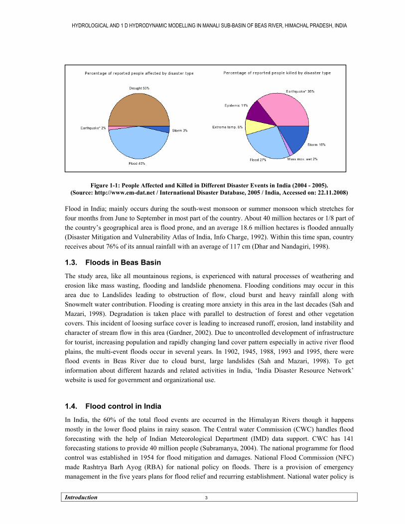
Flood is the most common natural disaster in India, even in the world. It causes more damage in terms of loss of life property and economic activity than any other natural disaster (FEMA, 2000)2. India occupies a place as one of the most disaster prone country in world map where flood is on the in the series of disasters. According to International Disaster Database (EM-DAT, 2008), there were 305 and 360 natural disasters within which 107 and 168 were flood disaster in 2004 and 2005 respectively throughout the world where India listed as 2nd position suffering from 30 natural disasters. According to EM-DAT statistics, total 74, 285, 072 and 116, 990, 371 populations was affected and 6135 and 6957 were killed shares 6.1 % and 13.7 % of total killed population in the above years. There were huge damage and loss due to several flood disasters in India, like Himachal Pradesh, 1988, Orissa, 1999, 2006, 2008, West Bengal 2000, 2004, Maharashtra, 2005, Gujrat, 2007, Saharsa area near Nepal etc. in addition with the every year flood hazard in low lying Gangetic plain in India (Parasuraman and Unnikrishnan P, 2000). Due to lack of planning and development, knowledge, protection, techniques and devices for economy, political benefit and pressure of geometrically grown population and their needs, this type of disaster is taking place almost every year. Some related historical statistics (2004 - 2005) of different disasters are given below in Figure 1-1 and the contribution of flood hazard is clear from the cartograms.
2 FEMA - Federal Emergency Management Agency
HYDROLOGICAL AND 1 D HYDRODYNAMIC MODELLING IN MANALI SUB-BASIN OF BEAS RIVER, HIMACHAL PRADESH, INDIA
Introduction 3
Figure 1-1: People Affected and Killed in Different Disaster Events in India (2004 - 2005).
(Source: http://www.em-dat.net / International Disaster Database, 2005 / India, Accessed on: 22.11.2008)
Flood in India; mainly occurs during the south-west monsoon or summer monsoon which stretches for four months from June to September in most part of the country. About 40 million hectares or 1/8 part of the country’s geographical area is flood prone, and an average 18.6 million hectares is flooded annually (Disaster Mitigation and Vulnerability Atlas of India, Info Charge, 1992). Within this time span, country receives about 76% of its annual rainfall with an average of 117 cm (Dhar and Nandagiri, 1998).
1.3. Floods in Beas Basin
The study area, like all mountainous regions, is experienced with natural processes of weathering and erosion like mass wasting, flooding and landslide phenomena. Flooding conditions may occur in this area due to Landslides leading to obstruction of flow, cloud burst and heavy rainfall along with Snowmelt water contribution. Flooding is creating more anxiety in this area in the last decades (Sah and Mazari, 1998). Degradation is taken place with parallel to destruction of forest and other vegetation covers. This incident of loosing surface cover is leading to increased runoff, erosion, land instability and character of stream flow in this area (Gardner, 2002). Due to uncontrolled development of infrastructure for tourist, increasing population and rapidly changing land cover pattern especially in active river flood plains, the multi-event floods occur in several years. In 1902, 1945, 1988, 1993 and 1995, there were flood events in Beas River due to cloud burst, large landslides (Sah and Mazari, 1998). To get information about different hazards and related activities in India, ‘India Disaster Resource Network’ website is used for government and organizational use.
1.4. Flood control in India
In India, the 60% of the total flood events are occurred in the Himalayan Rivers though it happens mostly in the lower flood plains in rainy season. The Central water Commission (CWC) handles flood forecasting with the help of Indian Meteorological Department (IMD) data support. CWC has 141 forecasting stations to provide 40 million people (Subramanya, 2004). The national programme for flood control was established in 1954 for flood mitigation and damages. National Flood Commission (NFC) made Rashtrya Barh Ayog (RBA) for national policy on floods. There is a provision of emergency management in the five years plans for flood relief and recurring establishment. National water policy is

HYDROLOGICAL AND 1 D HYDRODYNAMIC MODELLING IN MANALI SUB-BASIN OF BEAS RIVER, HIMACHAL PRADESH, INDIA
Introduction 4
also considered for all type of problems related with waters. National Disaster Management Authority (NDMA) under Home Affairs, Government of India, National Remote Sensing Agency (NRSA) and Department of Science and Technology (DST) are also engaged in working for natural hazard management and risk reduction.
1.5. Role of Remore Sensing in Hydrological and hydraulic Modeling
Hydrological and hydrodynamic modelling needs more accurate field measured data about several hydrological, hydrodynamic and basin data. There are several problems to collect adequate data from the field for time, space, economy and security constraints. Remote sensing images help to produce huge information in temporal and spatial domain with different resolutions. The aerial photography, multi-spectral space borne data, radar back scatter, LiDAR3 point data, Global Positioning System (GPS) reading help directly and indirectly to model the hydrological processes and flood related study in different scales. The never ending process of water cycle through the earth and atmosphere and its forecasting, evaluation, assessment, management is difficult and time consuming through conventional methods. The satellites like GOES4, INSAT5, TRMM6, NOAA7 etc. are used for cloud types, cloud top temperatures helps indirectly to predict rainfalls with the help of ground network of rain gauge measurements and some relevant developed algorithms. The very crucial key variables for the model are extracted without point measurement from remote sensing data with different spectral and spatial resolution. It provides the cost effective synoptic view of different spatial entities that help to create thematic maps of natural and man made resources like elevation, channel area, surface water, land use/land cover, soil moisture, vegetation, snow cover, evaporation etc. and their temporal changes. Distributed hydrological model combine with the remote sensing information provides hazard characteristics and their effects like water logging, soil erosion, flood height, velocity, inundated area etc. along with calibration and validation of the model. Topography controls the flow velocity and patterns of a basin. Topographic characteristics can be collected from Digital Elevation Model (DEM), Digital Surface Model (DSM) and Triangular Irregular Network (TIN) digitally.
1.6. Role of GIS in hydrological and hydraulic modeling
The subject of modelling is growingly undertaking the integration of spatial and non spatial information together. Modelling is increasingly used for water quality assessment, water supply, hazard related study, basin management and planning. Geographical information system (GIS) makes the large amount spatial data possible to store, retrieve, correction or manage the complex problem first. Then it helps to analyze the required GIS input for predetermined output layers for different purpose. The geomorphology, land cover, cross section etc. can be seen in different dimension, layers and corrected as requires. In most of the cases remote sensing data are indirectly used for hydrological modelling. So, for digital image processing, thematic map layers generation for input key variables, GIS are obvious to integrate the user and the computer to provide spatial information which helps according to the needs. It takes considerable time to compute and give results with GIS outputs spatial and non-spatial data simultaneously. The user interface is also helpful for GIS experts and friendly to update and more temporal.
3 LiDAR – Light Detection and Ranging, 4 GOES – Geostationary Satellite, USA. 5 INSAT – Indian National Satellite, India. 6 TRMM – Tropical Rainfall Measuring Mission, Japan. 7 NOAA – National Oceanic and Atmospheric Administration, USA.
HYDROLOGICAL AND 1 D HYDRODYNAMIC MODELLING IN MANALI SUB-BASIN OF BEAS RIVER, HIMACHAL PRADESH, INDIA
Introduction 5
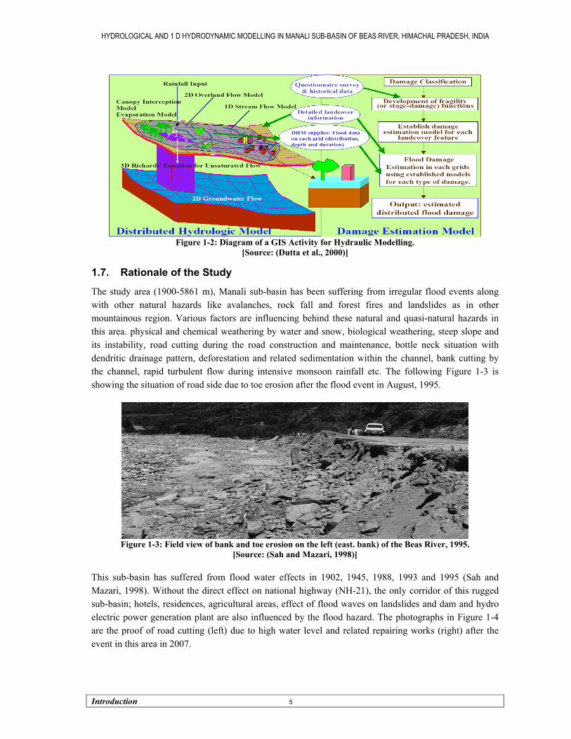
Figure 1-2: Diagram of a GIS Activity for Hydraulic Modelling.
[Source: (Dutta et al., 2000)]
1.7. Rationale of the Study
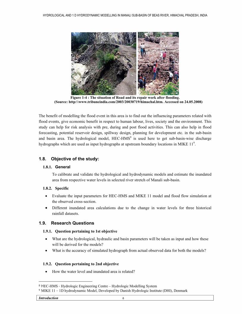
The study area (1900-5861 m), Manali sub-basin has been suffering from irregular flood events along with other natural hazards like avalanches, rock fall and forest fires and landslides as in other mountainous region. Various factors are influencing behind these natural and quasi-natural hazards in this area. physical and chemical weathering by water and snow, biological weathering, steep slope and its instability, road cutting during the road construction and maintenance, bottle neck situation with dendritic drainage pattern, deforestation and related sedimentation within the channel, bank cutting by the channel, rapid turbulent flow during intensive monsoon rainfall etc. The following Figure 1-3 is showing the situation of road side due to toe erosion after the flood event in August, 1995.
Figure 1-3: Field view of bank and toe erosion on the left (east. bank) of the Beas River, 1995.
[Source: (Sah and Mazari, 1998)]
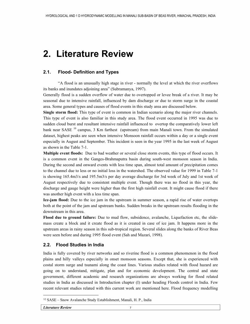
This sub-basin has suffered from flood water effects in 1902, 1945, 1988, 1993 and 1995 (Sah and Mazari, 1998). Without the direct effect on national highway (NH-21), the only corridor of this rugged sub-basin; hotels, residences, agricultural areas, effect of flood waves on landslides and dam and hydro electric power generation plant are also influenced by the flood hazard. The photographs in Figure 1-4 are the proof of road cutting (left) due to high water level and related repairing works (right) after the event in this area in 2007.
HYDROLOGICAL AND 1 D HYDRODYNAMIC MODELLING IN MANALI SUB-BASIN OF BEAS RIVER, HIMACHAL PRADESH, INDIA
Introduction 6
Figure 1-4 : The situation of Road and its repair work after flooding.
(Source: http:\\www.tribuneindia.com/2003/20030719/himachal.htm. Accessed on 24.05.2008)
The benefit of modelling the flood event in this area is to find out the influencing parameters related with flood events, give economic benefit in respect to human labour, lives, society and the environment. This study can help for risk analysis with pre, during and post flood activities. This can also help in flood forecasting, potential reservoir design, spillway design, planning for development etc. in the sub-basin and basin area. The hydrological model, HEC-HMS8 is used here to get sub-basin-wise discharge hydrographs which are used as input hydrographs at upstream boundary locations in MIKE 119.
1.8. Objective of the study:
1.8.1. General
To calibrate and validate the hydrological and hydrodynamic models and estimate the inundated area from respective water levels in selected river stretch of Manali sub-basin.
1.8.2. Specific
• Evaluate the input parameters for HEC-HMS and MIKE 11 model and flood flow simulation at the observed cross-section.
• Different inundated area calculations due to the change in water levels for three historical rainfall datasets.
1.9. Research Questions
1.9.1. Question pertaining to 1st objective
• What are the hydrological, hydraulic and basin parameters will be taken as input and how these will be derived for the models?
• What is the accuracy of simulated hydrograph from actual observed data for both the models?
1.9.2. Question pertaining to 2nd objective
• How the water level and inundated area is related?
8 HEC-HMS - Hydrologic Engineering Centre – Hydrologic Modelling System 9 MIKE 11 – 1D hydrodynamic Model, Developed by Danish Hydrologic Institute (DHI), Denmark
HYDROLOGICAL AND 1 D HYDRODYNAMIC MODELLING IN MANALI SUB-BASIN OF BEAS RIVER, HIMACHAL PRADESH, INDIA
Literature Review 7
2. Literature Review
2.1. Flood- Definition and Types
“A flood is an unusually high stage in river - normally the level at which the river overflows its banks and inundates adjoining area” (Subramanya, 1997). Generally flood is a sudden overflow of water due to overtopped or levee break of a river. It may be seasonal due to intensive rainfall, influenced by dam discharge or due to storm surge in the coastal area. Some general types and causes of flood events in this study area are discussed below. Single storm flood: This type of event is common in Indian scenario along the major river channels. This type of event is also familiar in this study area. The flood event occurred in 1995 was due to sudden cloud burst and resultant intensive rainfall influenced to overtop the comparatively lower left bank near SASE 10 campus, 3 Km farthest (upstream) from main Manali town. From the simulated dataset, highest peaks are seen when intensive Monsoon rainfall occurs within a day or a single event especially in August and September. This incident is seen in the year 1995 in the last week of August as shown in the Table 7-1. Multiple event floods: Due to bad weather or several close storm events, this type of flood occurs. It is a common event in the Ganges-Brahmaputra basin during south-west monsoon season in India. During the second and onward events with less time span, almost total amount of precipitation comes to the channel due to less or no initial loss in the watershed. The observed value for 1999 in Table 7-1 is showing 165.4m3/s and 195.5m3/s per day average discharge for 3rd week of July and 1st week of August respectively due to consistent multiple event. Though there was no flood in this year, the discharge and gauge height were higher than the first high rainfall event. It might cause flood if there was another high event with a less time span. Ice-jam flood: Due to the ice jam in the upstream in summer season, a rapid rise of water overtops both at the point of the jam and upstream banks. Sudden breaks in the upstream results flooding in the downstream in this area. Flood due to ground failure: Due to mud flow, subsidence, avalanche, Liquefaction etc, the slide-mass create a block and it create flood as it is created in case of ice jam. It happens more in the upstream areas in rainy season in this sub-tropical region. Several slides along the banks of River Beas were seen before and during 1995 flood event (Sah and Mazari, 1998).
2.2. Flood Studies in India
India is fully covered by river networks and so riverine flood is a common phenomenon in the flood plains and hilly valleys especially in onset monsoon seasons. Except that, she is experienced with costal storm surge and tsunami along the coast lines. Various studies related with flood hazard are going on to understand, mitigate, plan and for economic development. The central and state government, different academic and research organizations are always working for flood related studies in India as discussed in Introduction chapter (I) under heading Floods control in India. Few recent relevant studies related with this current work are mentioned here. Flood frequency modelling 10 SASE – Snow Avalanche Study Establishment, Manali, H. P., India

HYDROLOGICAL AND 1 D HYDRODYNAMIC MODELLING IN MANALI SUB-BASIN OF BEAS RIVER, HIMACHAL PRADESH, INDIA
Literature Review 8
using Curve Number (CN) and Kinematic wave method was examined in three un-gauged sub-basins in Indian scenario (Kurothe et al., 2001b). One study on 1D hydraulic modelling was done with MIKE 11 for parameterization and validation in Bagmoti River, Sikim (Agrawal et al., 2001). The controlling geomorphic element for flood events was done using Unit Hydrograph method in Kosi River, Bihar (Jain and Sinha, 2003). Here they clearly discussed about the factors which are more responsible behind frequent floods in Kosi River, the sorrow of Bihar. Dam failure and simulated flood analysis was done using MIKE 11 for hydro-electric project in Kameng District, Arunachal Pradesh (Husain and Rai, 2004). Baishya (2004) had used MIKE SHE to model the various hydrological component of Umium hilly catchment (223.05 Sq Km.), Meghalaya, India and described various method like functional and structural classification by level of spatial dis-aggregation and their advantages and disadvantages. They recommended that the land use/cover and slope play a vital role in enhancing the runoff. HEC-GeoRAS is used for generating the river network, cross section and GIS database for Mahanadi south east delta using ASTER DEM and field observed river cross section data for HEC-RAS11 model (Thakur and Sumangala, 2006). The land use land cover (LULC) map was prepared from IRS-LISS-3 data and used for assigning the Manning's N value. (Mohapatra and Sing, 2003) had discussed about the problems and management of flood hazards by four zones in India i. e. Brahmaputra River basin, Ganga River Basin, North-West River basin and Central India & Deccan River Basin.
2.3. Related Studies in Beas Basin
The study area is situated in a high elevated region and flood events are not frequent in the region. Due to cloud burst and funnel shaped dendritic stream network, the area suffered from various flood events several times. Several projects by central government are being implemented to reduce the possibility of flood as well as hazard caused by landslide, rock fall, debris flow etc. A few hydrological and flood inundation modelling is done by few Indian scholars in this area. Hydrological modelling of Beas basin was done for estimating PET12, AET13, surface runoff calculation, estimation of discharge, flood routing and water balance (Mahadev and Prasad, 2001). They found the balance of actual and potential evapo-transpiration for the whole year (for 2000 and 2001) where AET and PET vary from 0.2-1.4 mm and 0.6-2.7 mm respectively. They have also shown the snowmelt water contribution as 2 mm to 18 mm in winter and summer season respectively and a surplus of snowmelt and rain water in the Beas basin by water balance calculation. The (Jaiswal et al., 2003) have done L-Moment based flood frequency modeling in Beas basin. They tested statistical distributions to estimate the probable floods for Beas basin with both the probabilistic and deterministic approach. Prasad and Roy (2005) have also done a hydrological analysis for snow-melt water contribution in Beas River using snowmelt runoff model. They found the percentage of snow melt water throughout the year. Kumar et al. (2007) worked on snow and glacier melt contribution in the Beas River from historical records at Pandoh dam, Himachal Pradesh, India. They showed the snow and glacier melt runoff contributes about 35% to the annual flow of the Beas River with initial loss parameters. No such hydrodynamic modelling is successfully done in this study area except few hydrological modelling works with snow melt water contribution. So, it is a first attempt where both hydrological and hydraulic modelling are done and snowmelt water is also taken into account.
11 HEC-RAS – Hydrologic Engineering Centre – River Analysis System. 12 PET – Potential Evapo-transpiration. 13 AET – Actual Evapo-transpiration.
HYDROLOGICAL AND 1 D HYDRODYNAMIC MODELLING IN MANALI SUB-BASIN OF BEAS RIVER, HIMACHAL PRADESH, INDIA
Literature Review 9
2.4. Modelling-Definition and Types
Model is basically a representation of reality. Modelling of phenomenon and real happening is always a ‘miniature’ or the functions of a group of mathematical equations. These equations are not sufficient to represent the total complexity of real world rather than the simplification (Karssenberg, 2002; Van Loon and Jakob, 2005). Though models give more generalized view of basin hydraulics of the real world, (a) these are more advanced, capable, functional scope, multi activities, efficient models are coming continuously and are improving their work status as per requirement; (b) these can handle huge amount of data sets for large drainage networks with a limited time and cost; (c) easy user interface and most of the recent models are with GIS platform. Visualization of input and output with different dimension is possible here and the input error can be corrected and updated continuously in GIS layers. The effective modelling depends upon experience; selection of appropriate model and it is not a replacement of fieldwork which may help to make a better outcome. All models can not operate or give appropriate result in various spatiotemporal environments though they are made for same purpose. Models for physical process are open and accepted by scientific community.
2.4.1. Types of hydrological and Hydraulic models:
(A) Based on types: I. Physical vs. Mathematical vs. Numerical,
II. Empirical vs. Mathematical, III. Deterministic vs. Stochastic vs. Conceptual, IV. Steady vs. Unsteady, V. Based on Biological assumptions and
VI. Based on Hydrologic assumptions. (B) Models on their bases:
I. Function – Perspective and Descriptive, II. Structure – White box, Black box and Gray box,
III. Level of spatial disaggregating – Lumped and Distributed.
2.5. Hydrological Modelling
2.5.1. Choice of Model
These types of models are mathematical or symbolic representation of known or assumed functions which express the related components of hydrological cycle. Different types of hydrological models are being used depending upon the purpose throughout the world. HEC-HMS is a freeware and familiar model for hydrological simulation (Kurothe et al., 2001a). HEC-HMS is suitable for dendritic drainage pattern and it can include various parameters (HEC-HMS Reference Manual, 2000). So, this semi-distributed mathematical model is used here to get input hydrographs for hydraulic model at upstream boundary cross sections and to quantify the contribution of snowmelt water using the observed three annual rainfall and temperature records. More accurate datasets are needed for acceptable results from the model. So, the intensive field studies for reference, high resolution satellite data for physiography and LULC, sufficient observed gauge and hydro-meteorological datasets are necessary to run and validation of the model (Maidment, 1993; Wilson, 1996).

HYDROLOGICAL AND 1 D HYDRODYNAMIC MODELLING IN MANALI SUB-BASIN OF BEAS RIVER, HIMACHAL PRADESH, INDIA
Literature Review 10
2.5.2. Input Parameters and Outputs
Depending upon the physical, chemical or biological parameters and characteristics, it simulates the original hydrological processes of the catchments or basins (Cunge et al., 1980). The input parameters like slope, aspect, stream lines, junction, sub-basins, length of the reach, area, shape and outlet of the sub-basins, physiography, LULC, HSG14, CN, obstruction (n), base flow, loss and snow-melt rate etc. are derived and collected from satellite imageries, field survey and from literature with the help of GIS platform (HEC-HMS User’s Manual, 2000). Meteorological parameters like precipitation, temperature are collected mostly from measured datasets. Inflow, outflow, combined flow with snow melt water, loss for each sub-basin have been modelled according to purpose and availability of input data in HEC-HMS for three years i. e. 1995, 1999 and 2000. It is validated with observed data at Manali outlet only because of the availability of the observed data at this particular point. The detail procedure of parameterization, sensitivity analysis, calibration and validation are discussed in Methodology and Result and Discussion chapters (Chapter VI and VII).
2.6. Hydrodynamic Modelling
2.6.1. Choice of Models
The MIKE 11, a robust six point distributed 1D model is used for unsteady hydraulic to calculate the gauge height at the cross sections modelling (Bates and De Roo, 2000; DHI, 2008). It as not a freeware and a group of MIKE softwares work in MIKE Zero-based environment. It has a robust HD module and works in all relief conditions. Due to the availability of this model, it is used for this study. Here all the input files are generated in different file formats graphically as described in MIKE 11 User’s Manual, 2008. HEC-GeoRAS, compatible in Arc-View and Arc-Info is used for GIS layer preparation for network and cross section locations shape files. MIKE 11 is used to get water level, flood depth, discharge, rating curve, peak discharge at each cross section to generate hazard map.
2.6.2. Input Parameters and Outputs
The basic inputs of this hydraulic model are divided into four categories or files; network, cross section, boundary and hydrodynamic. In general, the parameters of hydraulic flood model are the representing topography or cross section, the layout of drainage, input discharge or boundary condition and others like reach lengths, roughness, initial flow etc. The drainage network is derived from ASTER DEM with the help pf topographical sheet, cross sections are measured from field, and the boundary parameters are taken from HEC-HMS output. The roughness co-efficient or Manning’s ‘N’ is calculated according to literature and field survey datasets for flow routing and used in HEC-GeoHMS linked TR55 worksheet for calculation of overland sheet flow and channel flows time of concentration (Chow et al., 1988; HEC-HMS Reference Manual, 2000). Then boundary conditions are fixed for unsteady flow simulations. For unsteady simulation, flow hydrographs curves are set for respective input upstream locations (main channel and tributaries) and Q-H15 relation is needed at the end cross section. This relation and base flow are collected from field survey and observed discharge. The gauge height or water level, water depth, discharge rate and volume, rating curve at different cross sections and mid point of two cross sections along the reaches are the output of this hydraulic model (Chapter VI).
14 HSG – Hydrological Soil Group 15 Q-H – Discharge-Gauge Height
HYDROLOGICAL AND 1 D HYDRODYNAMIC MODELLING IN MANALI SUB-BASIN OF BEAS RIVER, HIMACHAL PRADESH, INDIA
Literature Review 11
2.7. Sensitivity analysis and validation
Sensitivity analysis is also necessary for accurate flow dynamics, ranking of parameters and their comparative study (Aronica et al., 1998; Bates, 2004; Pappenberger et al., 2008). So it is an obvious criterion for the acceptance of the model. The Sensitivity is done here for both the models. Several authors have suggested about validating the model though it depends upon the study, model type and area. The observed data is used to compare the simulated result, so the availability of data is a most important criterion here. Validations of the models are done only for Manali outlet with the observed two years datasets (1999 and 2000). For more detail, see Chapter VI.
2.8. Use of DEM in hydrological modelling
The DEM pixel size has an important role in hydrological modelling. Low resolution DEM always gives the average and less information about the small features and land surface areas of complex relief those effects on local slope values, surface flow, lag time etc. ASTER DEM is used here for HEC-HMS model and no DEM is used in hydraulic modelling for this highly rugged topography because of their low resolution.
2.9. Consequence of Snow-melt Water in Flood Modelling
The base flow is contributed by mostly snow melt water in this study area. The snow melt water is ensuring perennial character of the main rivers throughout the year here. Temperature Index is used in hydrological model for simulated six months in this study to get the snow melt contribution in the total output discharge.
2.10. Scale Determination
It’s a one of the most important criteria for dynamic modelling. It determines the characteristics of the datasets, reliability, hypothesis and accuracy of the study (van Westen et al., 2000). The sensitivity of the model to different parameters varies depending upon the scale of study. The amount and availability of datasets, required processing time are also considered before fixing the scale of a study. The current hydrological modelling is done for a sub-basin (Manali) and Palchan to Manali, an eight Km stretch is used for hydraulic modelling part.
HYDROLOGICAL AND 1 D HYDRODYNAMIC MODELLING IN MANALI SUB-BASIN OF BEAS RIVER, HIMACHAL PRADESH, INDIA
Study Area 12
3. Study Area
3.1. Background
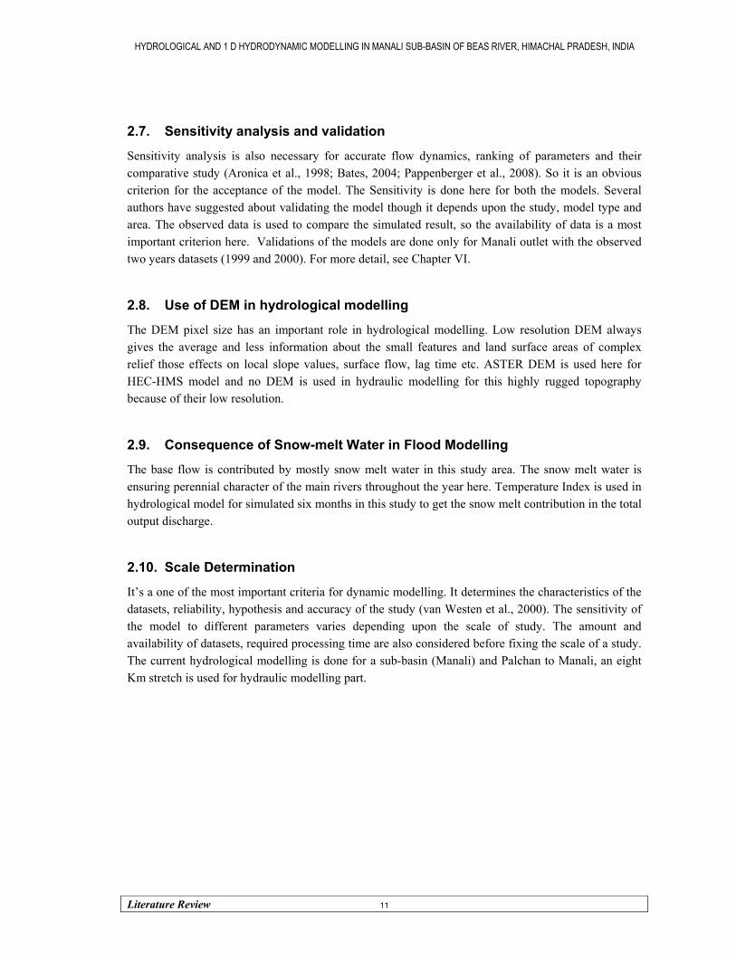
Manali Sub-basin, the study area is situated at the north in Kullu district between 32.230 N-32.420 N and 77.050 -77.280 E, Himachal Pradesh (HP) in India. The main sites of the area are Manali (2000 m), Palchan (2320 m) and Solang (2480 m), Dhundi (2800 m), Beas Kund (3690 m) and other stations are Kothi (2530 m), Marhi (3340 m), Rohtang Pass (3980 m), Bashist (2050 m), and Bhrigu Lake (4250 m). The sub-basin as well as the valley is a part of the Beas River, one of the tributaries of Indus river system. It has an area of 350 Km2 is part a part of “Valley of Gods” because of its religious and scenic places. The Beas river starts from Beas Kund (a small ice body) at an elevation of 4038 m on the eastern slope of Rohtang pass in the western Himalayas. It flows about north-south direction and takes a turn near Larji (957 meter) towards west in a right angle towards west and then it maintains its flow again north-south and west direction up to Pando dam (Singh, 1992). The area is surrounded by different districts of Himachal Pradesh like Kangra and Mandi in the east, Lahul and Spiti in the north and north-east side, Kinnaur and Shimla in the south-eastern part.
Figure 3-1: Location map of the Beas Sub-basin
Western Himalayan Region
INDIA
Jammu & Kashmir
HP
Uttarakhand Hills
BEAS KUND DHUNDI
PALCHAN
MANALI
PALCHAN
MANALI
Area – 350 Sq Km. & Scale - 1:470000
320 13’ 48’’ N 770 17’ E
320 25’ N 770 01’ 30’’ E
Manali to Palchan Stretch Manali Sub-basin
HYDROLOGICAL AND 1 D HYDRODYNAMIC MODELLING IN MANALI SUB-BASIN OF BEAS RIVER, HIMACHAL PRADESH, INDIA
Study Area 13
3.2. Geological Settings
The area is mainly composed of Pre-Cambrian Phylite, Schist, Gneiss and Granite. There is two geological formations namely, the Chail, newer and the Jutough, the older formation. Stratigraphically this area enjoys the reverse sequence i.e. Jutough formation is lying over the Chail as Nappe (Kullu Nappe) due to extreme pressure force during fold formation by Orogenic earth movement in Himalayan region (Mehta, 1976). Volcanic and metamorphic rocks are structured as banded sequence in these folded structures. This area is under higher categories of earthquake zone (Zone V) and many of the rivers start their flows along a fault line (Shankar and Dua, 1978; Virdi, 1979). The gap due to thrust and strike-slip fault allows percolation of rain water and recharges the ground water and increase seepage activity in the comparatively lower altitude whereas sub-surface permafrost environment is created in same geological structure in the cooperatively higher elevation. So, the geology of this area primarily controls the channel location and geometry, influences the elements of hydrological cycle, specially the ground water table, seepage, affluent nature of the channels etc. The inter banded structure with soft (mica) and hard rocks (granite, sandstone) causes sometimes slope failure due to more infiltration, weathering accelerated instability of slope and as a result; the landslide, rock slide etc. are happened frequently along river banks. This is also mentioned in Literature review chapter (Chapter II) in causes of flood section. Moreover in the upstream areas, flow velocity of the rivers is normally high because they are flowing through deep gorge with a higher gradient (Sah and Mazari, 1998). It takes less lag time which creates a high risk of flood, generated near the outlet (bottle neck) due to more accumulative flow.
3.3. General Geomorphology
The region presents asymmetric interlocking spar mosaic formed by the mountains and valleys within an elevation of 1900 - 5861 meters in both sides of the channel. The Beas valley is surrounded by Pir Panjal Range of lesser Himalaya in the north, Great Himalayan Range in the east, Dhawladhar Range in the south and Ravi valley is situated in the west. White snow capped mountain peaks are the landmark except urban places in this area. Glacial-fluvial process and weathering are predominant exogenetic forces to sculpture the morphology of this area. The upper concave and lower steep valleys form a curvilinear profile from downstream to upstream. Quaternary alluvial fans, originated from glacial and glacial-fluvial actions some time makes the channel and flood plains narrow. The toe erosion is more where alluvial fans are converged towards the channel and it frequently creates small slide as well as the water rise due to slide- jam (Singh, 1992).
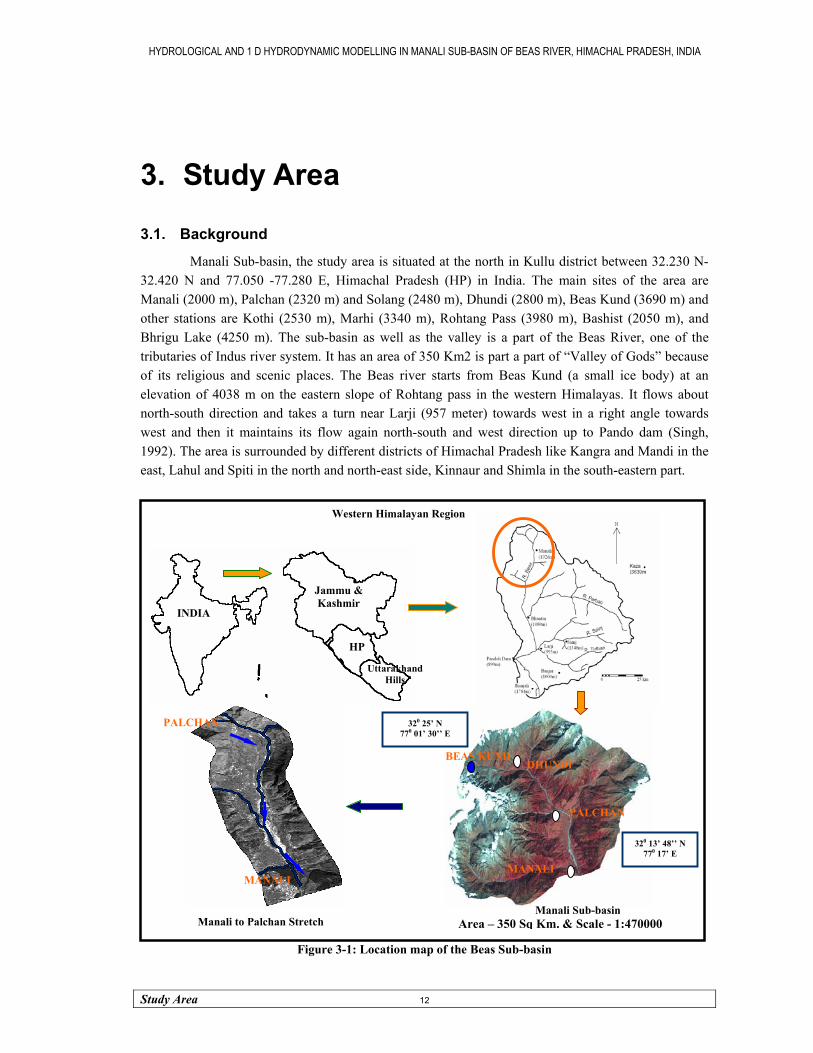
Figure 3-2: Focus towards Hill from River Beas at Beas Nalla, November, 2008.
HYDROLOGICAL AND 1 D HYDRODYNAMIC MODELLING IN MANALI SUB-BASIN OF BEAS RIVER, HIMACHAL PRADESH, INDIA
Study Area 14
3.4. Surface water potential
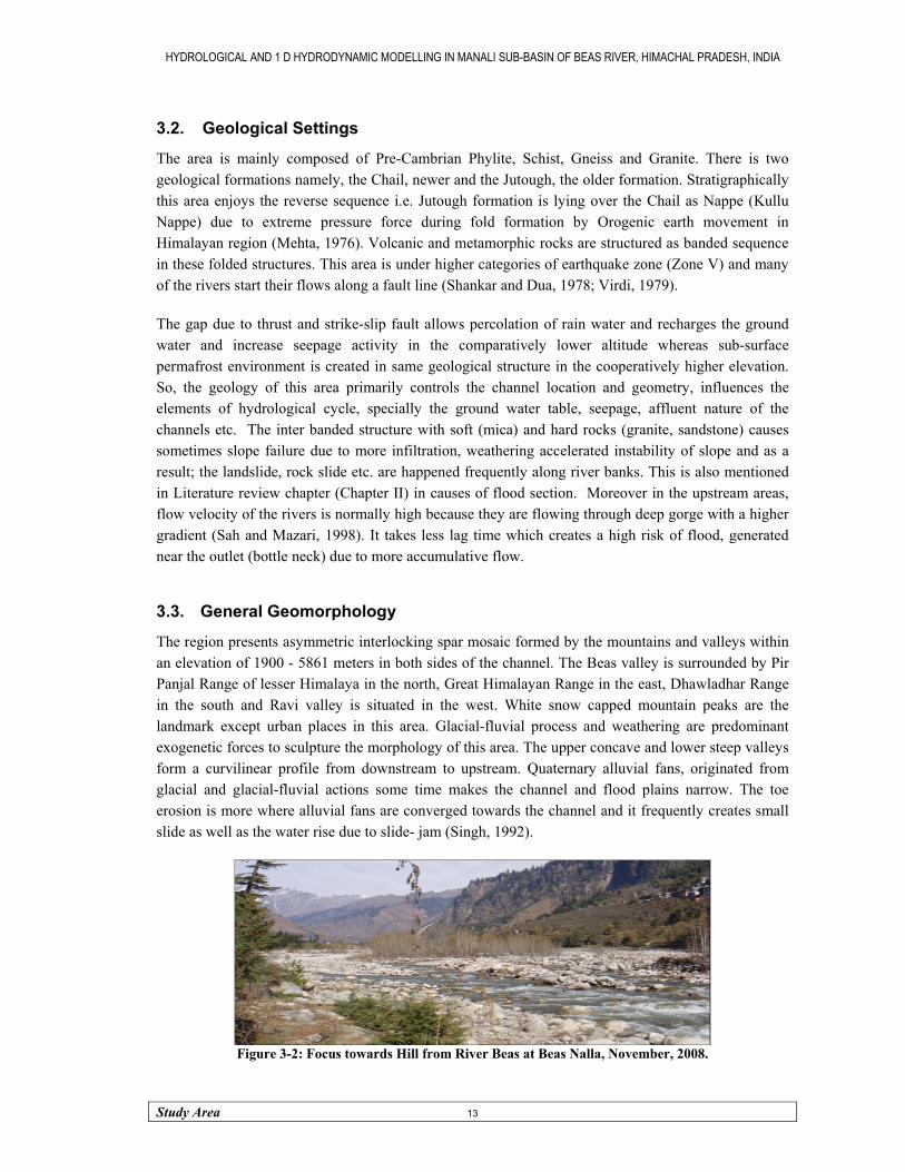
Water being a natural component has an important role for the places where it belongs to. The main sources of the surface water in this area are rivers, glaciers, springs, lakes, rainfall and snowfall in winter season. The main river Beas rises from famous “Beas Kund” where the great Vyas Rishi performed ‘tapa’ here during Mahabharata Kal at the Rohtang pass (above 4000m), in the Pir Panjal Range. Its names are Arjikiya in Vedic and Vipasa in Sanskrit. It flows for about 256 Km. in Himachal up to the plains at Mirthal. Three of the five tributaries in the Indus river system are flowing through the Himachal Pradesh and the Beas or Vipasa is one of them with many tributaries namely the Parbati, the Hurla, the Sainj, the Tirthan, the Uhl, the Suketi, the Luni, the Awa, the Banganga, the Manuni, the Gaj, the Chaki (Singh, 1992). The Beas River and its tributaries are affluent and perennial in nature except the southern are seasonal. No any tributaries are flowing in the current study area but some main nala (Palchan, Beas, RB SASE and Manalsu), jhora join with the Beas River which will be under consideration in this study. The snows melt and seepage water is considered as base in the channels.
Figure 3-3: River Beas near Manali and Beas Nalla, November, 2008.
One hot spring Vashist (2100 m) and two lakes – Beas Kund (3690 m) and Bhrigu lake (4270 m) are the another source of surface water in this area. The Bhrigu Lake over tops during the summer season because both snow-melt water and rainfall are then stored cumulatively with a large amount. The evapo-transpiration rate is not more because of alpine (acicular leaf) type of vegetation, less duration of sunlight and seasonal cloud, fog cover in this area. Another source of surface water is glaciers and a portion is covered by snow during the winter season because of elevation (November-February). A thin narrow snow melt water flow (base flow) is observed in the main channel in this time. Wide flow occurs due to more snow melt and cloud burst water which causes a high gauge at certain stretches with a considerable slope and height in summer season (March-September). It also causes falls, slides, bank erosion etc. during the same season. The following Table 4-1 is showing seasonal and total distribution of flow at Pandoh dam. The monsoon season contributes largest amount (4.09 km3) of discharge (55.1%) whereas the winter season has a lowest contribution of only 0.53 Km3 of discharge (7.2%) out of 7.42 Km3 of total discharge in average. Table 3-1: Average Seasonal Distribution of Annual Flows of the Beas River at Pandoh Dam.
Seasons Months Flow (km3) Flow (%)
Winter January–March 0.53 7.2
Pre-monsoon April–June 2.13 28.6
Monsoon July–September 4.09 55.1 Post-monsoon October–December 0.68 9.1
Total Whole Year 7.42 100
[Source: (Kumar et al., 2007)]

HYDROLOGICAL AND 1 D HYDRODYNAMIC MODELLING IN MANALI SUB-BASIN OF BEAS RIVER, HIMACHAL PRADESH, INDIA
Study Area 15
3.5. Ground water
The area is categorized as a ‘hard rock aquifer regime’ due to the rock types and stratigraphy as discussed in geological settings of this area (Baishya, 2004). Only the seasonal snow less and shale rich areas enjoy a deep ground water potential storage. The fracture, joints, more weathering based ground water recharge and channel based influent recharge are more effortful to uplift water table in this mountainous area. The depth of water table is variable depending upon the topography, stratigraphic set-up. The height of the water table varies within 5-15 m. under unconfined, semi confined or confined condition.
3.6. Climate
The area enjoys much varied climatic behaviour according to its elevation difference (1900 - 4250 m). The area experiences generally low normal monthly maximum temperature due to its altitude. After the month of June (hottest) the temperature continues to fall and the lowest temperature is experienced in January. The mean temperature rises above 20ºc during the summer months while lowest temperature falls below 2ºc in January in average though it goes in negative (Singh, 1992).
Figure 3-4: Annual Average Temperature and Rainfall.
(Source: http://www.world66.com/asia/southasia/himachalpradeshindia/manali/lib/climate, Accessed on 12.11.2008)
Figure 3-5: Weather in August, 2008 at 15:00 Hours.
The relative humidity is higher in the pre-monsoon (May, June) and monsoon period (July, August and September) and lower in winter season. About 70% of the annual rainfall is obtained during monsoon season for the cloud burst. Average annual rainfall is 100cm. Kothi is a meteorological unit here in this area. The climate is cold in general though it varies .for the differences in elevation and aspects and effect of global warming is also observed from the breakout of increasing diseases, insects and other hydro meteorological events. Sudden cloud burst, intensive rainfall in the monsoon season can create devastating flood event in this funnel shaped basin.
D
HYDROLOGICAL AND 1 D HYDRODYNAMIC MODELLING IN MANALI SUB-BASIN OF BEAS RIVER, HIMACHAL PRADESH, INDIA
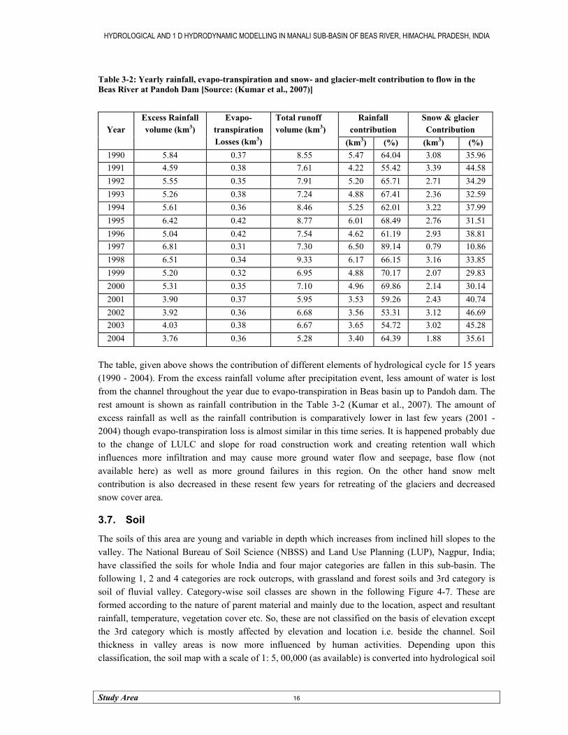
Study Area 16
Table 3-2: Yearly rainfall, evapo-transpiration and snow- and glacier-melt contribution to flow in the Beas River at Pandoh Dam [Source: (Kumar et al., 2007)]
Rainfall
contribution Snow & glacier Contribution
Year
Excess Rainfall volume (km3)
Evapo-transpiration Losses (km3)
Total runoff volume (km3)
(km3) (%) (km3) (%) 1990 5.84 0.37 8.55 5.47 64.04 3.08 35.96 1991 4.59 0.38 7.61 4.22 55.42 3.39 44.58 1992 5.55 0.35 7.91 5.20 65.71 2.71 34.29 1993 5.26 0.38 7.24 4.88 67.41 2.36 32.59 1994 5.61 0.36 8.46 5.25 62.01 3.22 37.99 1995 6.42 0.42 8.77 6.01 68.49 2.76 31.51 1996 5.04 0.42 7.54 4.62 61.19 2.93 38.81 1997 6.81 0.31 7.30 6.50 89.14 0.79 10.86 1998 6.51 0.34 9.33 6.17 66.15 3.16 33.85 1999 5.20 0.32 6.95 4.88 70.17 2.07 29.83 2000 5.31 0.35 7.10 4.96 69.86 2.14 30.14 2001 3.90 0.37 5.95 3.53 59.26 2.43 40.74 2002 3.92 0.36 6.68 3.56 53.31 3.12 46.69 2003 4.03 0.38 6.67 3.65 54.72 3.02 45.28 2004 3.76 0.36 5.28 3.40 64.39 1.88 35.61
The table, given above shows the contribution of different elements of hydrological cycle for 15 years (1990 - 2004). From the excess rainfall volume after precipitation event, less amount of water is lost from the channel throughout the year due to evapo-transpiration in Beas basin up to Pandoh dam. The rest amount is shown as rainfall contribution in the Table 3-2 (Kumar et al., 2007). The amount of excess rainfall as well as the rainfall contribution is comparatively lower in last few years (2001 -2004) though evapo-transpiration loss is almost similar in this time series. It is happened probably due to the change of LULC and slope for road construction work and creating retention wall which influences more infiltration and may cause more ground water flow and seepage, base flow (not available here) as well as more ground failures in this region. On the other hand snow melt contribution is also decreased in these resent few years for retreating of the glaciers and decreased snow cover area.
3.7. Soil
The soils of this area are young and variable in depth which increases from inclined hill slopes to the valley. The National Bureau of Soil Science (NBSS) and Land Use Planning (LUP), Nagpur, India; have classified the soils for whole India and four major categories are fallen in this sub-basin. The following 1, 2 and 4 categories are rock outcrops, with grassland and forest soils and 3rd category is soil of fluvial valley. Category-wise soil classes are shown in the following Figure 4-7. These are formed according to the nature of parent material and mainly due to the location, aspect and resultant rainfall, temperature, vegetation cover etc. So, these are not classified on the basis of elevation except the 3rd category which is mostly affected by elevation and location i.e. beside the channel. Soil thickness in valley areas is now more influenced by human activities. Depending upon this classification, the soil map with a scale of 1: 5, 00,000 (as available) is converted into hydrological soil

HYDROLOGICAL AND 1 D HYDRODYNAMIC MODELLING IN MANALI SUB-BASIN OF BEAS RIVER, HIMACHAL PRADESH, INDIA
Study Area 17
group map for SCS16 CN calculation for HEC-HMS hydrological model. The detail about CN calculation is discussed in Chapter VI.
Figure 3-6: Soil Map of Manali Sub-basin with a Scale of 1: 5, 00, 000
(Source: NBSS & LUP, Nagpur, India)
3.8. Natural vegetation
The landscape of Manali is occupied with Himalayan moist temperate and mixed forest within 2000-3500mts. Deodar and Kail are the most valuable timber forest in this category with silver fir and spruce (at 50-55mt ht.) species along the “Nallas” (small streams) extensively. The moist deciduous forest between 2000-3000 mates is found in this area. Alder species are seen up to 2250mts on the unstable hills and moist ravines (Singh, 1992). The costly edible and nuts producer pine species, mountain bamboo are also seen with Chil pine below 2200mts height in the study area. The total forest area is 140 hectare (Tahsil office, Manali, 2008). Long grasses and orchards found in 4th group of soil, as described above, mainly during rainy season for their elevated location. Depending upon the vegetation type near the banks and deposited bar, roughness coefficients are determined along the cross sections with the help of field survey and widely accepted literature (Acrement and Schneider, 1989).
Figure 3-7: Pine forest and apple Orchards, November, 2008.
16 SCS – Soil Conservation Service, USA.
Soil Map of Manali Sub-basin
HYDROLOGICAL AND 1 D HYDRODYNAMIC MODELLING IN MANALI SUB-BASIN OF BEAS RIVER, HIMACHAL PRADESH, INDIA
Study Area 18
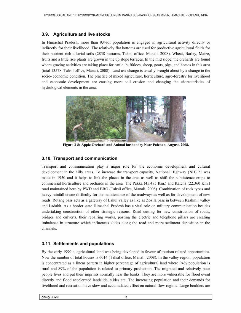
3.9. Agriculture and live stocks
In Himachal Pradesh, more than 93%of population is engaged in agricultural activity directly or indirectly for their livelihood. The relatively flat bottoms are used for productive agricultural fields for their nutrient rich alluvial soils (2838 hectares, Tahsil office, Manali, 2008). Wheat, Barley, Maize, fruits and a little rice plants are grown in the up slope terraces. In the mid slope, the orchards are found where grazing activities are taking place for cattle, buffaloes, sheep, goats, pigs, and horses in this area (total 13578, Tahsil office, Manali, 2008). Land use change is usually brought about by a change in the socio- economic condition. The practice of mixed agriculture, horticulture, agro-forestry for livelihood and economic development are causing more soil erosion and changing the characteristics of hydrological elements in the area.
Figure 3-8: Apple Orchard and Animal husbandry Near Palchan, August, 2008.
3.10. Transport and communication
Transport and communication play a major role for the economic development and cultural development in the hilly areas. To increase the transport capacity, National Highway (NH) 21 was made in 1950 and it helps to link the places in the area as well as shift the subsistence crops to commercial horticulture and orchards in the area. The Pakka (45.485 Km.) and Katcha (22.360 Km.) road maintained here by PWD and BRO (Tahsil office, Manali, 2008). Combination of rock types and heavy rainfall create difficulty for the maintenance of the roadways as well as for development of new roads. Rotang pass acts as a gateway of Lahul valley as like as Zozila pass in between Kashmir valley and Ladakh. As a border state Himachal Pradesh has a vital role on military communication besides undertaking construction of other strategic reasons. Road cutting for new construction of roads, bridges and culverts, their repairing works, posting the electric and telephone pillars are creating imbalance in structure which influences slides along the road and more sediment deposition in the channels.
3.11. Settlements and populations
By the early 1990’s, agricultural land was being developed in favour of tourism related opportunities. Now the number of total houses is 6014 (Tahsil office, Manali, 2008). In the valley region, population is concentrated as a linear pattern in higher percentage of agricultural land where 94% population is rural and 89% of the population is related to primary production. The migrated and relatively poor people lives and put their imprints normally near the banks. They are more vulnerable for flood event directly and flood accelerated landslide, slides etc. The increasing population and their demands for livelihood and recreation have slow and accumulated effect on natural flow regime. Large boulders are

HYDROLOGICAL AND 1 D HYDRODYNAMIC MODELLING IN MANALI SUB-BASIN OF BEAS RIVER, HIMACHAL PRADESH, INDIA
Study Area 19
thrown away towards the channel from the upper hill to make agricultural terraces. Pandoh dam is constructed to fulfil the demand of people. Due to the location of this dam and its storage, the flow in upper catchment is affected. Many pipe lines are made from up-hill to settled areas to collect the fresh water, melted from glacier. This procedure makes unstable the area as well as affects the base flow throughout the year. Surface flow during the precipitation is increasing for decreasing vegetation cover which effects ground water table. Low ground water table can make the soil more fragile due to decreasing cohesion and it influences slope failure and jam in the channel. To increase the tourist demand and economy, inaccessible places of virgin natural beauty are being accessible cutting the trees, making the roads etc. and as a result the temperature is rising and it influences to retreat glaciers, decreasing snow melt discharge i. e. base flow throughout the year.
Figure 3-9: Settlements along the Beas River, November, 2008.
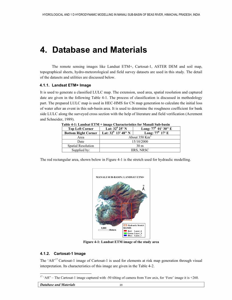
HYDROLOGICAL AND 1 D HYDRODYNAMIC MODELLING IN MANALI SUB-BASIN OF BEAS RIVER, HIMACHAL PRADESH, INDIA
Database and Materials 20
4. Database and Materials
The remote sensing images like Landsat ETM+, Cartosat-1, ASTER DEM and soil map, topographical sheets, hydro-meteorological and field survey datasets are used in this study. The detail of the datasets and utilities are discussed below.
4.1.1. Landsat ETM+ Image
It is used to generate a classified LULC map. The extension, used area, spatial resolution and captured date are given in the following Table 4-1. The process of classification is discussed in methodology part. The prepared LULC map is used in HEC-HMS for CN map generation to calculate the initial loss of water after an event in this sub-basin area. It is used to determine the roughness coefficient for bank side LULC along the surveyed cross section with the help of literature and field verification (Acrement and Schneider, 1989).
Table 4-1: Landsat ETM + image Characteristics for Manali Sub-basin Top Left Corner Lat: 320 25’ N Long: 770 01' 30'' E
Bottom Right Corner Lat: 320 13' 48'' N Long: 770 17' E Area About 350 Km2 Date 15/10/2000
Spatial Resolution 30 m Supplied by: IIRS, NRSC
The red rectangular area, shown below in Figure 4-1 is the stretch used for hydraulic modelling.
Figure 4-1: Landsat ETM image of the study area
4.1.2. Cartosat-1 Image
The ‘Aft’17 Cartosat-1 image of Cartosat-1 is used for elements at risk map generation through visual interpretation. Its characteristics of this image are given in the Table 4-2.
17 ‘Aft” – The Cartosat-1 image captured with -50 tilting of camera from Yaw axis, for ‘Fore’ image it is +260.
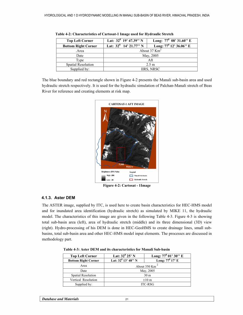
HYDROLOGICAL AND 1 D HYDRODYNAMIC MODELLING IN MANALI SUB-BASIN OF BEAS RIVER, HIMACHAL PRADESH, INDIA
Database and Materials 21
Table 4-2: Characteristics of Cartosat-1 Image used for Hydraulic Stretch The blue boundary and red rectangle shown in Figure 4-2 presents the Manali sub-basin area and used hydraulic stretch respectively. It is used for the hydraulic simulation of Palchan-Manali stretch of Beas River for reference and creating elements at risk map.
Figure 4-2: Cartosat - 1Image
4.1.3. Aster DEM
The ASTER image, supplied by ITC, is used here to create basin characteristics for HEC-HMS model and for inundated area identification (hydraulic stretch) as simulated by MIKE 11, the hydraulic model. The characteristics of this image are given in the following Table 4-3. Figure 4-3 is showing total sub-basin area (left), area of hydraulic stretch (middle) and its three dimensional (3D) view (right). Hydro-processing of his DEM is done in HEC-GeoHMS to create drainage lines, small sub-basins, total sub-basin area and other HEC-HMS model input elements. The processes are discussed in methodology part.
Table 4-3: Aster DEM and its characteristics for Manali Sub-basin
Top Left Corner Lat: 320 19’ 47.39’’ N Long: 770 08’ 31.60’’ E Bottom Right Corner Lat: 320 14’ 21.77’’ N Long: 770 12’ 36.06’’ E
.Area About 37 Km2 Date May, 2005 Type Aft
Spatial Resolution 2.5 m Supplied by: IIRS, NRSC
Top Left Corner Lat: 320 25’ N Long: 770 01’ 30’’ E Bottom Right Corner Lat: 320 13’ 48’’ N Long: 770 17’ E
Area About 350 Km 2 Date May, 2005
Spatial Resolution 30 m Vertical Resolution ±10 m
Supplied by: ITC-RSG

HYDROLOGICAL AND 1 D HYDRODYNAMIC MODELLING IN MANALI SUB-BASIN OF BEAS RIVER, HIMACHAL PRADESH, INDIA
Database and Materials 22
Figure 4-3: ASTER DEM for Manali Sub-basin and Hydraulic stretch with its 3D View
4.1.4. Topo-Sheet
Except these above remote sensing images, three consecutive Topo-sheets (52H/3, 52H/4 and 52H/7 with a 1:50,000 scale) are used for survey guides, cross section location of cross sections and total Manali sub-basin boundary identification. These SOI18 topographical sheets are supplied by IIRS.
4.1.5. Soil Map
The whole soil map of Himachal Pradesh jointly prepared by National Bureau of Soil Science (NBSS) and Land Use Department (LUP), Nagpur Centre with 1:5, 00,000 scales has been used to prepare Hydrological Soil Group (HSG) map for hydrological simulation. The soil classes are shown in Figure 4-4 below.
Figure 4-4: Soil Map of the Study Area
18 SOI – Survey of India
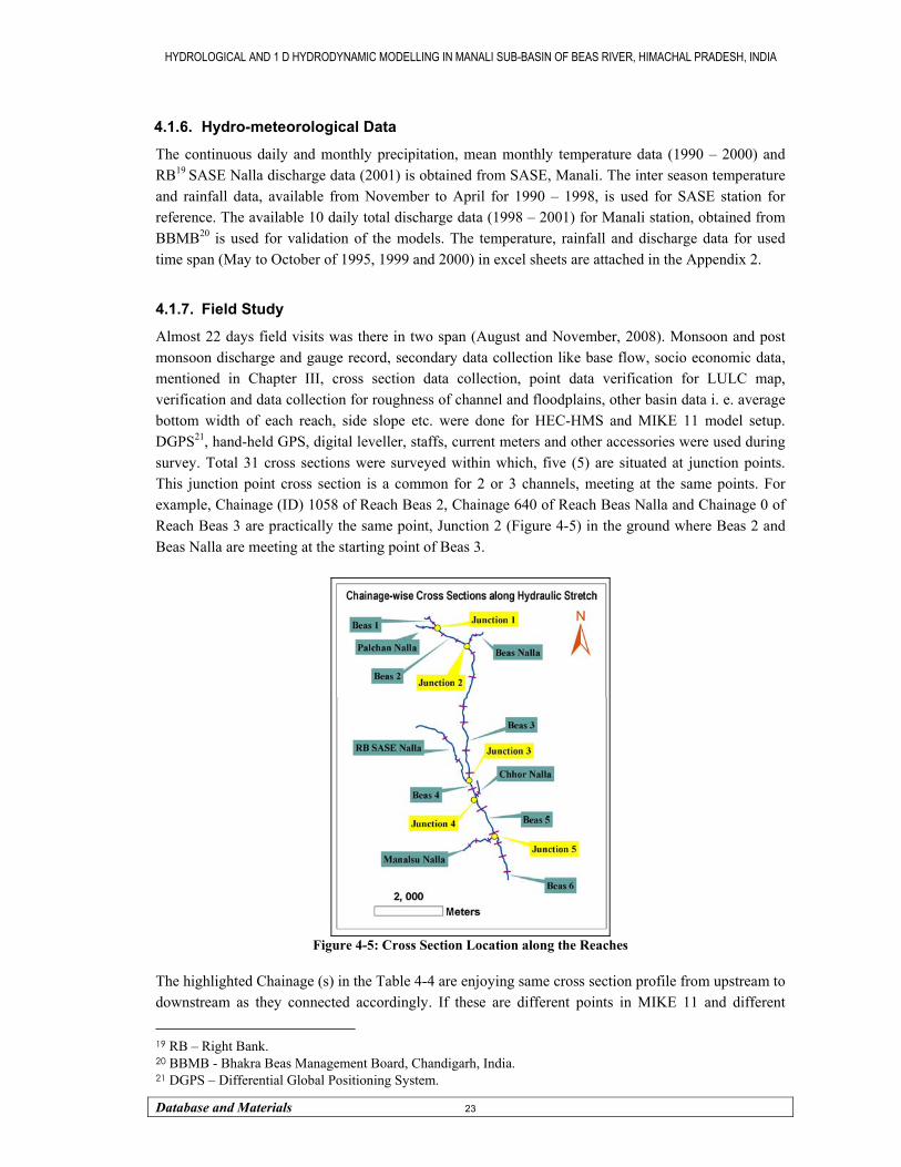
HYDROLOGICAL AND 1 D HYDRODYNAMIC MODELLING IN MANALI SUB-BASIN OF BEAS RIVER, HIMACHAL PRADESH, INDIA
Database and Materials 23
4.1.6. Hydro-meteorological Data
The continuous daily and monthly precipitation, mean monthly temperature data (1990 – 2000) and RB19 SASE Nalla discharge data (2001) is obtained from SASE, Manali. The inter season temperature and rainfall data, available from November to April for 1990 – 1998, is used for SASE station for reference. The available 10 daily total discharge data (1998 – 2001) for Manali station, obtained from BBMB20 is used for validation of the models. The temperature, rainfall and discharge data for used time span (May to October of 1995, 1999 and 2000) in excel sheets are attached in the Appendix 2.
4.1.7. Field Study
Almost 22 days field visits was there in two span (August and November, 2008). Monsoon and post monsoon discharge and gauge record, secondary data collection like base flow, socio economic data, mentioned in Chapter III, cross section data collection, point data verification for LULC map, verification and data collection for roughness of channel and floodplains, other basin data i. e. average bottom width of each reach, side slope etc. were done for HEC-HMS and MIKE 11 model setup. DGPS21, hand-held GPS, digital leveller, staffs, current meters and other accessories were used during survey. Total 31 cross sections were surveyed within which, five (5) are situated at junction points. This junction point cross section is a common for 2 or 3 channels, meeting at the same points. For example, Chainage (ID) 1058 of Reach Beas 2, Chainage 640 of Reach Beas Nalla and Chainage 0 of Reach Beas 3 are practically the same point, Junction 2 (Figure 4-5) in the ground where Beas 2 and Beas Nalla are meeting at the starting point of Beas 3.
Figure 4-5: Cross Section Location along the Reaches
The highlighted Chainage (s) in the Table 4-4 are enjoying same cross section profile from upstream to downstream as they connected accordingly. If these are different points in MIKE 11 and different
19 RB – Right Bank. 20 BBMB - Bhakra Beas Management Board, Chandigarh, India. 21 DGPS – Differential Global Positioning System.
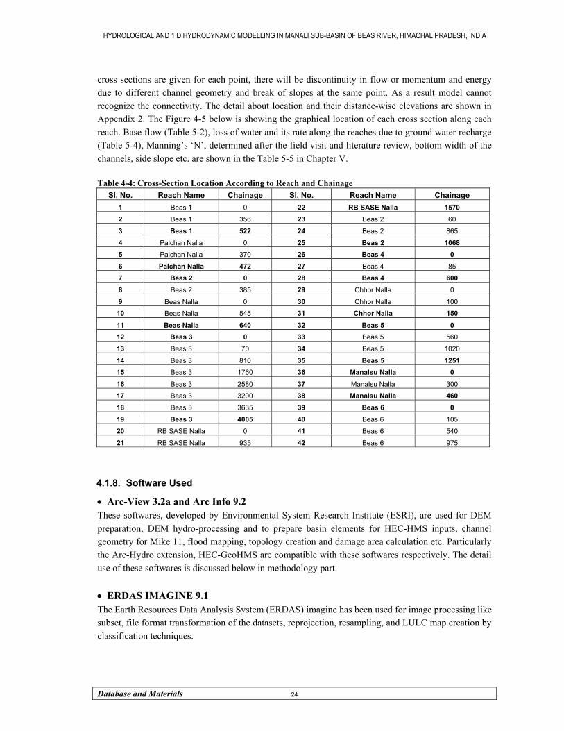
HYDROLOGICAL AND 1 D HYDRODYNAMIC MODELLING IN MANALI SUB-BASIN OF BEAS RIVER, HIMACHAL PRADESH, INDIA
Database and Materials 24
cross sections are given for each point, there will be discontinuity in flow or momentum and energy due to different channel geometry and break of slopes at the same point. As a result model cannot recognize the connectivity. The detail about location and their distance-wise elevations are shown in Appendix 2. The Figure 4-5 below is showing the graphical location of each cross section along each reach. Base flow (Table 5-2), loss of water and its rate along the reaches due to ground water recharge (Table 5-4), Manning’s ‘N’, determined after the field visit and literature review, bottom width of the channels, side slope etc. are shown in the Table 5-5 in Chapter V. Table 4-4: Cross-Section Location According to Reach and Chainage
Sl. No. Reach Name Chainage Sl. No. Reach Name Chainage 1 Beas 1 0 22 RB SASE Nalla 1570 2 Beas 1 356 23 Beas 2 60
3 Beas 1 522 24 Beas 2 865
4 Palchan Nalla 0 25 Beas 2 1068 5 Palchan Nalla 370 26 Beas 4 0 6 Palchan Nalla 472 27 Beas 4 85
7 Beas 2 0 28 Beas 4 600 8 Beas 2 385 29 Chhor Nalla 0
9 Beas Nalla 0 30 Chhor Nalla 100
10 Beas Nalla 545 31 Chhor Nalla 150 11 Beas Nalla 640 32 Beas 5 0 12 Beas 3 0 33 Beas 5 560
13 Beas 3 70 34 Beas 5 1020
14 Beas 3 810 35 Beas 5 1251 15 Beas 3 1760 36 Manalsu Nalla 0 16 Beas 3 2580 37 Manalsu Nalla 300
17 Beas 3 3200 38 Manalsu Nalla 460 18 Beas 3 3635 39 Beas 6 0 19 Beas 3 4005 40 Beas 6 105
20 RB SASE Nalla 0 41 Beas 6 540
21 RB SASE Nalla 935 42 Beas 6 975
4.1.8. Software Used
• Arc-View 3.2a and Arc Info 9.2 These softwares, developed by Environmental System Research Institute (ESRI), are used for DEM preparation, DEM hydro-processing and to prepare basin elements for HEC-HMS inputs, channel geometry for Mike 11, flood mapping, topology creation and damage area calculation etc. Particularly the Arc-Hydro extension, HEC-GeoHMS are compatible with these softwares respectively. The detail use of these softwares is discussed below in methodology part. • ERDAS IMAGINE 9.1 The Earth Resources Data Analysis System (ERDAS) imagine has been used for image processing like subset, file format transformation of the datasets, reprojection, resampling, and LULC map creation by classification techniques.

HYDROLOGICAL AND 1 D HYDRODYNAMIC MODELLING IN MANALI SUB-BASIN OF BEAS RIVER, HIMACHAL PRADESH, INDIA
Database and Materials 25
• HEC-HMS 3.1.0 and HEC-GeoHMS 1.1 This is U.S. Army Crops of Engineers’ Hydrologic Modelling System and it’s a free ware for dendritic watershed system. It is used for hydrologic simulation of Manali sub-basin to prepare input hydrographs of contributing un-gauged small streams meeting in the main Beas River. It is the upper version of 2.2.2 with more functionality like snow melt contribution calculation. HEC-GeoHMS, compatible with Arc-View, is used to create GIS layers of the sub-basin. The detail of input and output is discussed in Chapter VI and VII. • MIKE 11 This one dimensional hydraulic modelling software, developed by Danish Hydrologic Institute (DHI), Denmark is based on MIKE Zero support. The geometric input is primarily taken from HEC-GeoRAS as shape files. The channel network and cross section files are different in it. Its input, calibration, output and validation results are discussed below in Chapter VI and VII. • Other Software There was a major support of MS Excel, Word and Power Point from the beginning. Some particular support of other image processing and GIS software was there for cross section data visualization, transferred from Digital Leveller and other example data processing.

HYDROLOGICAL AND 1 D HYDRODYNAMIC MODELLING IN MANALI SUB-BASIN OF BEAS RIVER, HIMACHAL PRADESH, INDIA
Methodology 26
5. Methodology
The whole study is subdivided into three parts: pre field, field and post field works. In pre-field study; literature review, material collection from secondary sources like Topo-sheets, remote sensing images, field preparation etc were done. Field survey activities are already discussed in chapter-V. Now the post-field activities i.e. Data-base preparation for model input, calibration, validation and inundated area calculation are discussed in this chapter.
5.1. HEC-HMS Model
The following Fig.6-1 is showing the post field activities related with HEC-HMS model.
Figure 5-1: Flow Chart of HEC-HMS Model
5.1.1. DEM Hydro-Processing
Before going to the HEC-HMS part, the terrain processing is needed to generate hydrological maps in other supported software like Arc-View for GeoHMS because there are no tools to edit, modify the DEM in GeoHMS itself. With the help of spatial and 3D analyst tool boxes, it can be done. There is other extension in Arc-GIS for DEM hydro processing like ‘Arc hydro tool’ in which this part is done, and then it is used in GeoHMS. The grid format is a must input file type for DEM and here 30 m. ASTER DEM is used for this pre GeoHMS hydro processing. The Several hydrological maps are generated step by step but in case of stream line generation, user specific threshold value is given. Giving 50 Km2 threshold values for watershed aggregation, 22 sub-watersheds are primarily formed and then these are merged into 7 sub-watersheds according to the availability of flow and cross section data. The following physical parameters are generated from DEM processing:
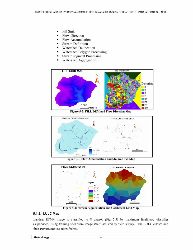
HYDROLOGICAL AND 1 D HYDRODYNAMIC MODELLING IN MANALI SUB-BASIN OF BEAS RIVER, HIMACHAL PRADESH, INDIA
Methodology 27
Fill Sink Flow Direction Flow Accumulation Stream Definition Watershed Delineation Watershed Polygon Processing Stream segment Processing Watershed Aggregation
Figure 5-2: FILL DEM and Flow Direction Map
Figure 5-3: Flow Accumulation and Stream Grid Map
Figure 5-4: Stream Segmentation and Catchment Grid Map
5.1.2. LULC Map
Landsat ETM+ image is classified to 8 classes (Fig 5-5) by maximum likelihood classifier (supervised) using training sites from image itself, assisted by field survey. The LULC classes and their percentages are given below.
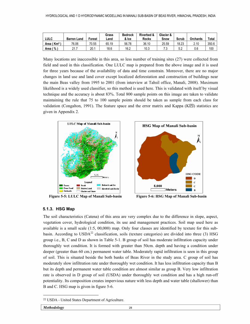
HYDROLOGICAL AND 1 D HYDRODYNAMIC MODELLING IN MANALI SUB-BASIN OF BEAS RIVER, HIMACHAL PRADESH, INDIA
Methodology 28
LULC Barren Land Forest Grass Land
Bedrock & Ice
Riverbed & Rocks
Glacier & Snow Scrub Orchards Total
Area ( Km2 ) 76.06 70.55 65.19 56.78 36.10 25.59 18.23 2.10 350.6 Area ( % ) 21.7 20.1 18.6 16.2 10.3 7.3 5.2 0.6 100
Many locations are inaccessible in this area, so less number of training sites (27) were collected from field and used in this classification. One LULC map is prepared from the above image and it is used for three years because of the availability of data and time constrain. Moreover, there are no major changes in land use and land cover except localized deforestation and construction of buildings near the main Beas valley from 1995 to 2001 (from interview at Tahsil office, Manali, 2008). Maximum likelihood is a widely used classifier, so this method is used here. This is validated with itself by visual technique and the accuracy is about 83%. Total 800 sample points on this image are taken to validate maintaining the rule that 75 to 100 sample points should be taken as sample from each class for validation (Congalton, 1991). The feature space and the error matrix and Kappa (K ) statistics are given in Appendix 2.
Figure 5-5: LULC Map of Manali Sub-basin Figure 5-6: HSG Map of Manali Sub-basin
5.1.3. HSG Map
The soil characteristics (Catena) of this area are very complex due to the difference in slope, aspect, vegetation cover, hydrological condition, its use and management practices. Soil map used here as available is a small scale (1:5, 00,000) map. Only four classes are identified by texture for this sub-basin. According to USDA22 classification, soils (texture categories) are divided into three (3) HSG group i.e., B, C and D as shown in Table 5-1. B group of soil has moderate infiltration capacity under thoroughly wet condition. It is formed with greater than 50cm. depth and having a condition under deeper (greater than 60 cm.) permanent water table. Moderately rapid infiltration is seen in this group of soil. This is situated beside the both banks of Beas River in the study area. C group of soil has moderately slow infiltration rate under thoroughly wet condition. It has less infiltration capacity than B but its depth and permanent water table condition are almost similar as group B. Very low infiltration rate is observed in D group of soil (USDA) under thoroughly wet condition and has a high run-off potentiality. Its composition creates impervious nature with less depth and water table (shallower) than B and C. HSG map is given in figure 5-6.
22 USDA - United States Department of Agriculture.
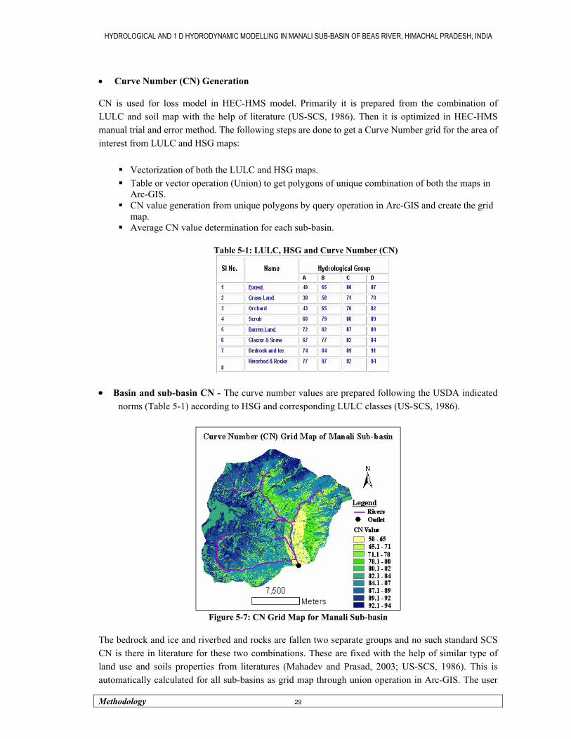
HYDROLOGICAL AND 1 D HYDRODYNAMIC MODELLING IN MANALI SUB-BASIN OF BEAS RIVER, HIMACHAL PRADESH, INDIA
Methodology 29
• Curve Number (CN) Generation CN is used for loss model in HEC-HMS model. Primarily it is prepared from the combination of LULC and soil map with the help of literature (US-SCS, 1986). Then it is optimized in HEC-HMS manual trial and error method. The following steps are done to get a Curve Number grid for the area of interest from LULC and HSG maps:
Vectorization of both the LULC and HSG maps. Table or vector operation (Union) to get polygons of unique combination of both the maps in
Arc-GIS. CN value generation from unique polygons by query operation in Arc-GIS and create the grid
map. Average CN value determination for each sub-basin.
Table 5-1: LULC, HSG and Curve Number (CN)
• Basin and sub-basin CN - The curve number values are prepared following the USDA indicated norms (Table 5-1) according to HSG and corresponding LULC classes (US-SCS, 1986).
Figure 5-7: CN Grid Map for Manali Sub-basin
The bedrock and ice and riverbed and rocks are fallen two separate groups and no such standard SCS CN is there in literature for these two combinations. These are fixed with the help of similar type of land use and soils properties from literatures (Mahadev and Prasad, 2003; US-SCS, 1986). This is automatically calculated for all sub-basins as grid map through union operation in Arc-GIS. The user

HYDROLOGICAL AND 1 D HYDRODYNAMIC MODELLING IN MANALI SUB-BASIN OF BEAS RIVER, HIMACHAL PRADESH, INDIA
Methodology 30
specified cell size is given to get unique average CN value for each cell. Statistics for each sub-basin are then created. This table can be used to identify the LULC-HSG combination of CN values which has largest impact on overall CN of sub-basins or water shades.
5.1.4. HEC-GeoHMS Processing
The following steps are done in HEC-GeoRAS with Arc-View window: • Starts New Project – The user defined project name. • Generate New Project – The total sub-basin (Manali) is demarcated using 1:50, 000 Survey of
India Topo-sheets, mentioned earlier. • Threshold Value for the project – Here the largest area of expected basin is given as 100 Km2.
using previous knowledge about area from Topo-sheets. The number of sub-watersheds is depending upon the threshold area value. Here 26 sub-basins are created automatically with a threshold value of 50 Km2. Then these sub-watersheds are merged and finally 7 sub-basins are created to get outflow hydrographs from HEC-HMS and these are the predefined upstream boundary input in MIKE 11. The outlet location is pointed manually and then the study area is automatically defined.
Figure 5-8: Catchment, Drainage and Main outlet of Manali Sub-basin with sub-ids.
• Basin Processing - Here small basins are merged intentionally to achieve the hydrographs of only predetermined particular locations with the help of Topographical sheets. The merging and splitting can be done from project viewer. Depending upon the purpose and characteristics of the basin (mainly shape), different methods are used for better result. The flow path method i. e. the centroid as the centre of longest flow path is used here. Another methods are Bounding box (centroid identified the bounded polygon) and Ellipse Method (centroid as the centre of the best fitted elliptical polygon). • Longest Flow Path – It computes the longest flow route in the whole basin or for all sub-basins for travelling time calculation done in the HEC-HMS.
62
30 37
41
80
84 72
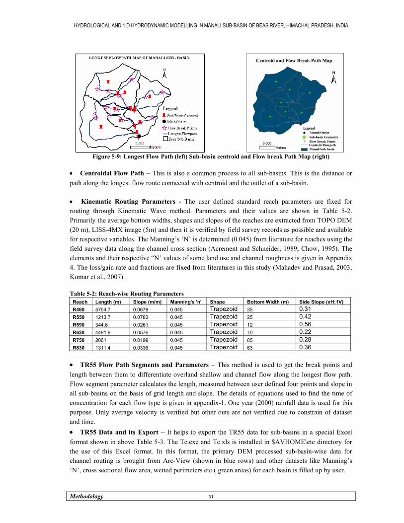
HYDROLOGICAL AND 1 D HYDRODYNAMIC MODELLING IN MANALI SUB-BASIN OF BEAS RIVER, HIMACHAL PRADESH, INDIA
Methodology 31
Figure 5-9: Longest Flow Path (left) Sub-basin centroid and Flow break Path Map (right)
• Centroidal Flow Path – This is also a common process to all sub-basins. This is the distance or path along the longest flow route connected with centroid and the outlet of a sub-basin. • Kinematic Routing Parameters - The user defined standard reach parameters are fixed for routing through Kinematic Wave method. Parameters and their values are shown in Table 5-2. Primarily the average bottom widths, shapes and slopes of the reaches are extracted from TOPO DEM (20 m), LISS-4MX image (5m) and then it is verified by field survey records as possible and available for respective variables. The Manning’s ‘N’ is determined (0.045) from literature for reaches using the field survey data along the channel cross section (Acrement and Schneider, 1989; Chow, 1995). The elements and their respective “N’ values of some land use and channel roughness is given in Appendix 4. The loss/gain rate and fractions are fixed from literatures in this study (Mahadev and Prasad, 2003; Kumar et al., 2007). Table 5-2: Reach-wise Routing Parameters
Reach Length (m) Slope (m/m) Manning's 'n' Shape Bottom Width (m) Side Slope (xH:1V) R460 5754.7 0.0679 0.045 Trapezoid 35 0.31 R550 1213.7 0.0783 0.045 Trapezoid 25 0.42 R590 344.6 0.0261 0.045 Trapezoid 12 0.56 R620 4481.9 0.0576 0.045 Trapezoid 70 0.22 R750 2061 0.0199 0.045 Trapezoid 85 0.28 R830 1311.4 0.0336 0.045 Trapezoid 63 0.36
• TR55 Flow Path Segments and Parameters – This method is used to get the break points and length between them to differentiate overland shallow and channel flow along the longest flow path. Flow segment parameter calculates the length, measured between user defined four points and slope in all sub-basins on the basis of grid length and slope. The details of equations used to find the time of concentration for each flow type is given in appendix-1. One year (2000) rainfall data is used for this purpose. Only average velocity is verified but other outs are not verified due to constrain of dataset and time. • TR55 Data and its Export – It helps to export the TR55 data for sub-basins in a special Excel format shown in above Table 5-3. The Tc.exe and Tc.xls is installed in $AVHOME\etc directory for the use of this Excel format. In this format, the primary DEM processed sub-basin-wise data for channel routing is brought from Arc-View (shown in blue rows) and other datasets like Manning’s ‘N’, cross sectional flow area, wetted perimeters etc.( green areas) for each basin is filled up by user.

HYDROLOGICAL AND 1 D HYDRODYNAMIC MODELLING IN MANALI SUB-BASIN OF BEAS RIVER, HIMACHAL PRADESH, INDIA
Methodology 32
Table 5-3: Worksheet according to TR55 Method
Then the output (in HEC-HMS) values are calculated by HEC-HMS as shown in white and yellow rows in Table 5-2. The sheet, shallow concentrated and channel flow equations are given in appendix 1. The merged watershed IDs are shown in Table 5-3 and Figure 5-8. The default values in green areas is changed as needed but values in white and yellow areas should not be modified because these are dependent on the other cells and its values are computed by TR55 excel sheet inbuilt formulas. It is stored automatically in the project directory as shown in 28th row in the table. The sub-basins and reach names are shown below in Figure 5-10 as sketched in HEC-HMS. The sub-divisions shown in this figure is adopted for the demand of upstream boundary conditions (hydrographs) in MIKE 11.
Figure 5-10: Sub-watersheds and Reaches
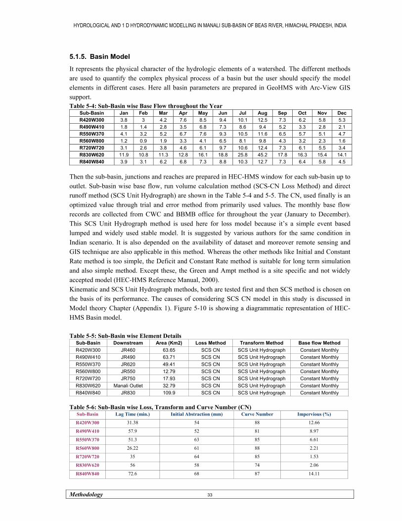
HYDROLOGICAL AND 1 D HYDRODYNAMIC MODELLING IN MANALI SUB-BASIN OF BEAS RIVER, HIMACHAL PRADESH, INDIA
Methodology 33
5.1.5. Basin Model
It represents the physical character of the hydrologic elements of a watershed. The different methods are used to quantify the complex physical process of a basin but the user should specify the model elements in different cases. Here all basin parameters are prepared in GeoHMS with Arc-View GIS support. Table 5-4: Sub-Basin wise Base Flow throughout the Year
Sub-Basin Jan Feb Mar Apr May Jun Jul Aug Sep Oct Nov Dec R420W300 3.8 3 4.2 7.6 8.5 9.4 10.1 12.5 7.3 6.2 5.8 5.3 R490W410 1.8 1.4 2.8 3.5 6.8 7.3 8.6 9.4 5.2 3.3 2.8 2.1 R550W370 4.1 3.2 5.2 6.7 7.6 9.3 10.5 11.6 6.5 5.7 5.1 4.7 R560W800 1.2 0.9 1.9 3.3 4.1 6.5 8.1 9.8 4.3 3.2 2.3 1.6 R720W720 3.1 2.6 3.8 4.6 6.1 9.7 10.6 12.4 7.3 6.1 5.5 3.4 R830W620 11.9 10.8 11.3 12.8 16.1 18.8 25.8 45.2 17.8 16.3 15.4 14.1 R840W840 3.9 3.1 6.2 6.8 7.3 8.8 10.3 12.7 7.3 6.4 5.8 4.5
Then the sub-basin, junctions and reaches are prepared in HEC-HMS window for each sub-basin up to outlet. Sub-basin wise base flow, run volume calculation method (SCS-CN Loss Method) and direct runoff method (SCS Unit Hydrograph) are shown in the Table 5-4 and 5-5. The CN, used finally is an optimized value through trial and error method from primarily used values. The monthly base flow records are collected from CWC and BBMB office for throughout the year (January to December). This SCS Unit Hydrograph method is used here for loss model because it’s a simple event based lumped and widely used stable model. It is suggested by various authors for the same condition in Indian scenario. It is also depended on the availability of dataset and moreover remote sensing and GIS technique are also applicable in this method. Whereas the other methods like Initial and Constant Rate method is too simple, the Deficit and Constant Rate method is suitable for long term simulation and also simple method. Except these, the Green and Ampt method is a site specific and not widely accepted model (HEC-HMS Reference Manual, 2000). Kinematic and SCS Unit Hydrograph methods, both are tested first and then SCS method is chosen on the basis of its performance. The causes of considering SCS CN model in this study is discussed in Model theory Chapter (Appendix 1). Figure 5-10 is showing a diagrammatic representation of HEC-HMS Basin model. Table 5-5: Sub-Basin wise Element Details
Sub-Basin Downstream Area (Km2) Loss Method Transform Method Base flow Method R420W300 JR460 63.65 SCS CN SCS Unit Hydrograph Constant Monthly R490W410 JR490 63.71 SCS CN SCS Unit Hydrograph Constant Monthly R550W370 JR620 49.41 SCS CN SCS Unit Hydrograph Constant Monthly R560W800 JR550 12.79 SCS CN SCS Unit Hydrograph Constant Monthly R720W720 JR750 17.93 SCS CN SCS Unit Hydrograph Constant Monthly R830W620 Manali Outlet 32.79 SCS CN SCS Unit Hydrograph Constant Monthly R840W840 JR830 109.9 SCS CN SCS Unit Hydrograph Constant Monthly
Table 5-6: Sub-Basin wise Loss, Transform and Curve Number (CN)
Sub-Basin Lag Time (min.) Initial Abstraction (mm) Curve Number Impervious (%)
R420W300 31.38 54 88 12.66
R490W410 57.9 52 81 8.97
R550W370 51.3 63 85 6.61
R560W800 26.22 61 88 2.21
R720W720 35 64 85 1.53
R830W620 56 58 74 2.06
R840W840 72.6 68 87 14.11

HYDROLOGICAL AND 1 D HYDRODYNAMIC MODELLING IN MANALI SUB-BASIN OF BEAS RIVER, HIMACHAL PRADESH, INDIA
Methodology 34
Primarily the Lag time is determined by TR55 method for each sub-basin. Initial abstraction (mm) is assumed first depending upon the percentage of impervious area and precipitation period, vegetation cover area, its type and temperature characteristics (Mahadev and Prasad, 2003). Impervious area is calculated from land use and land cover i. e. the summation of settlement and hard rock area and the CN is obtained from generated CN grid map, as discussed earlier (HEC-HMS Reference manual, 2000). Then these are optimized with performance result through trial and error method. The total Initial abstractions (IA) are kept constant for this continuous six months simulation because this simulation is done only for the rainy months and no ancillary datasets were available. The time distribution of this total initial abstraction is done as per amount of rainfall events in six months. The more percentages of this IA are given to initial rainy days of June and July, and lesser amounts of IA in august and later months. The reach parameters and routing method are given in Table 5-2 and 5-6 for respective reaches. Depending upon the dataset, used loss method, general characteristics of peak (single), shape, area and LULC type of the Sub-basins, the SCS Unit Hydrograph (UH), a parametric method is used here in this study for excess precipitation transformation (HEC-HMS Reference Manual, 2000). Constant loss rate and its fraction (Table 5-7) are determined by slope and composition of the bed material and soil (HEC-HMS Reference manual, 2000). The literature and information from CWC, Manali are used to get the particular values for each reach. Surface run-off excess from precipitation is calculated through SCS unit hydrograph and for channel routing, Kinematic wave method is used. Kinematic wave method is used here for flow routing. This method is selected for the present study due to very high reach slope, dendritic drainage pattern, no back water effect and supercritical flow is there in all reaches. The observed data set is available only for the outlet, so insufficiency of dataset for each sub-basin led to consider this method. The Muskingum Cunge method is tested first but it has given comparatively poor result (64% accuracy). The respective equations are shown in Appendix 1. Table 5-7: Reach-wise Element Details
Reach Downstream Routing Method Loss/Gain Method Flow Rate-m3/s (Loss) Fraction (Loss) R460 JR550 Kinematic Wave Constant 0.04 0.040 R550 JR620 Kinematic Wave Constant 0.05 0.060 R590 JR620 Kinematic Wave Constant 0.06 0.048 R620 JR750 Kinematic Wave Constant 0.06 0.060 R750 JR830 Kinematic Wave Constant 0.15 0.060 R830 Manali Outlet Kinematic Wave Constant 0.12 0.055
5.1.6. Meteorological Model
The input precipitation amount (point), temperature, snowmelt water contribution etc. are calculated in this part. Time series of daily precipitation and temperature data of 1995, 1999 and 2000 is the input for this study. Bahang SASE and Dhundi station data (point) are used as specified hydrographs in time series data window through manual input for 1995, 1999 and 2000 from May to October. The units for temperature and rainfall data are in degree centigrade and mm respectively. The snow melt runoff contribution is calculated from temperature index (TI). Though there are three stations in this study area, the meteorological data are used here only for two gauge stations because of the availability of datasets. The total area is subdivided into three elevation zones (Bands) in TI method. The meteorological gauges are assigned according to sub-basin locations as shown in the following Table 5-8 (left). No spatial interpolation method is used for weighted distribution of rainfall throughout the basin, as grid based daily rainfall maps could not be generated in HMS-DSS format. The individual sub-basin is fed with equal precipitation amount in this case. If the temperature is less than 0 degree in

HYDROLOGICAL AND 1 D HYDRODYNAMIC MODELLING IN MANALI SUB-BASIN OF BEAS RIVER, HIMACHAL PRADESH, INDIA
Methodology 35
any sub-basin, the form of precipitation is treated as snowfall instead of rainfall. Snowmelt water contribution is added according to ‘Temperature Index’ parameters (Table 5-8 and 5-9). Table 5-8: Sub-Basin wise Rainfall Gauge and Other Elements and Meteorological Model Set-Up
Table 5-9: Temperature Index Parameters
Parameters Value Parameters Value PX Temperature (DEG C) 0 Cold Limit (mm/DAY) 20 Base Temperature (DEG C) 0 ATI-Cold Rate Coefficient 0.84 Wet Melt Rate (mm/DEG C-DAY) 100 ATI-Cold Rate Function None Rain Rate Limit (mm/DAY) 10 Water Capacity (%) 5 ATI-Melt Rate Coefficient 0.98 Ground Melt Method Fixed Value ATI-Melt Rate Function Table ATI melt rate Ground Melt (mm/DAY) 50 Melt Rate Pattern None ----- -----
The temperature is given followed by universal normal lapse rate 6.4°c/km. The parameters, unit system is given in Table 5-8. The Temperature Index (TI) parameters (Table 5-9) are taken from SASE authority. These are strictly restricted datasets. On the basis of these data sets the TI parameters and values are given as input in paired data section. • Control Specification - It includes the starting and ending date, time and the duration of each simulation. The time span for starting and ending date (1st May to 31st October), computation time steps (one day) is specified here.
Start Date Start Time End Date End Time Time Interval
01 May, Year 0:00 31 Oct, Year 0:00 1 Day
5.1.7. ATI Melt Rate Function
This is calculated for snow melt runoff contribution from temperature index in HEC-HMS for each simulated year 1995. 1999 and 2000 from the months May to October depending upon the ATI parameters taken for ‘Manali Basin’. The parameters for ATI index and their values are given in Appendix 2.
5.1.8. Run the model
This HEC-HMS is calibrated with dataset of the year 2000 using the ‘Manali Basin’ framework. The model includes seven reaches, six junctions and seven sub-basins. The SCS Curve Number method is used for loss estimation, the SCS unit Hydrograph method is used for Transform computation and Kinematic Wave method is used is used for Routing purpose because of the terrain characteristics. The meteorological model and ‘Temperature Index’ for snow melt contribution include the specified
Sub-basin
Gauge
Lapse Rate (DEG/Km)
R420W300 Dhundi -6.4 R490W410 Bahang_SASE -6.4 R550W370 Dhundi -6.4 R560W800 Bahang_SASE -6.4 R720W720 Bahang_SASE -6.4 R830W620 Bahang_SASE -6.4 R840W840 Bahang_SASE -6.4
Precipitation
Specified Hyetograph
Snowmelt Temperature Index Unit System Metric
Basin Manali
Replace Missing Yes
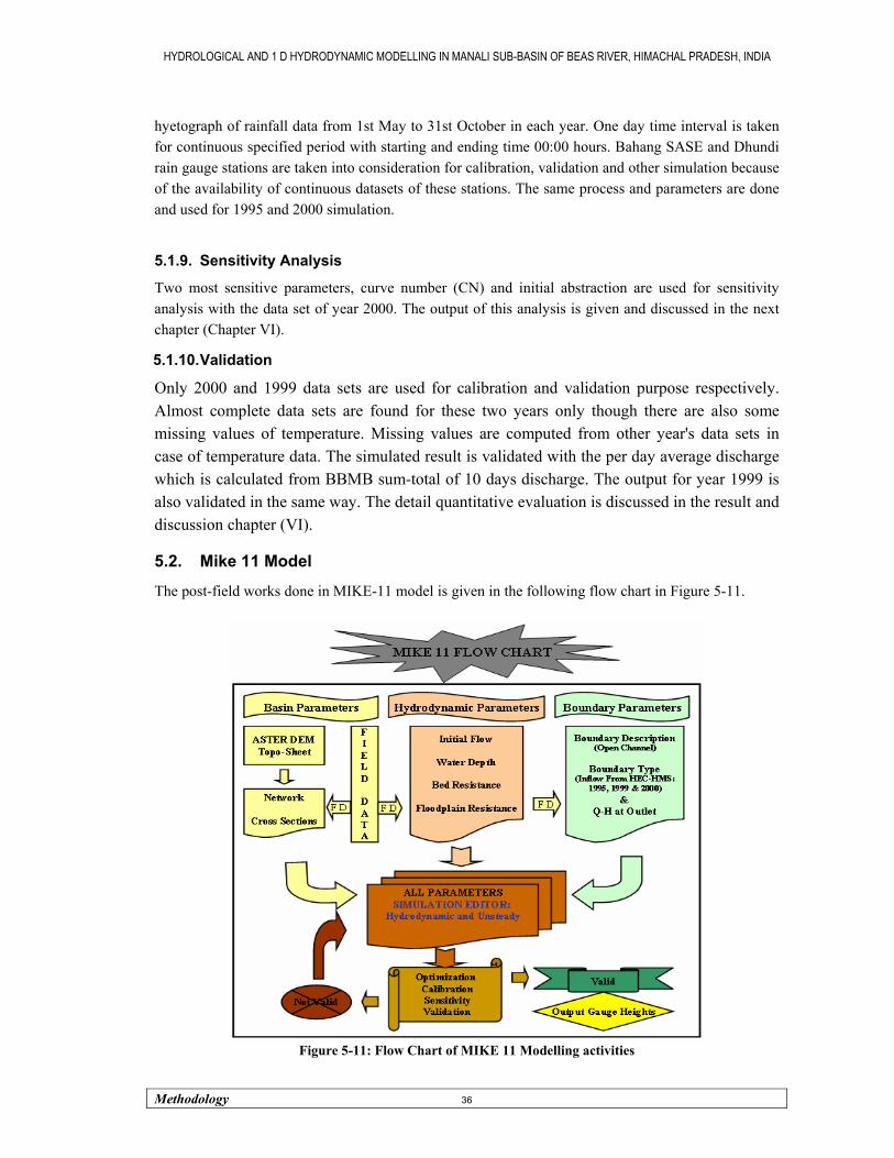
HYDROLOGICAL AND 1 D HYDRODYNAMIC MODELLING IN MANALI SUB-BASIN OF BEAS RIVER, HIMACHAL PRADESH, INDIA
Methodology 36
hyetograph of rainfall data from 1st May to 31st October in each year. One day time interval is taken for continuous specified period with starting and ending time 00:00 hours. Bahang SASE and Dhundi rain gauge stations are taken into consideration for calibration, validation and other simulation because of the availability of continuous datasets of these stations. The same process and parameters are done and used for 1995 and 2000 simulation.
5.1.9. Sensitivity Analysis
Two most sensitive parameters, curve number (CN) and initial abstraction are used for sensitivity analysis with the data set of year 2000. The output of this analysis is given and discussed in the next chapter (Chapter VI).
5.1.10. Validation
Only 2000 and 1999 data sets are used for calibration and validation purpose respectively. Almost complete data sets are found for these two years only though there are also some missing values of temperature. Missing values are computed from other year's data sets in case of temperature data. The simulated result is validated with the per day average discharge which is calculated from BBMB sum-total of 10 days discharge. The output for year 1999 is also validated in the same way. The detail quantitative evaluation is discussed in the result and discussion chapter (VI).
5.2. Mike 11 Model
The post-field works done in MIKE-11 model is given in the following flow chart in Figure 5-11.
Figure 5-11: Flow Chart of MIKE 11 Modelling activities
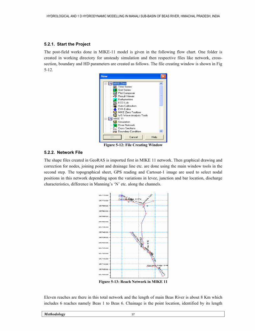
HYDROLOGICAL AND 1 D HYDRODYNAMIC MODELLING IN MANALI SUB-BASIN OF BEAS RIVER, HIMACHAL PRADESH, INDIA
Methodology 37
5.2.1. Start the Project
The post-field works done in MIKE-11 model is given in the following flow chart. One folder is created in working directory for unsteady simulation and then respective files like network, cross-section, boundary and HD parameters are created as follows. The file creating window is shown in Fig 5-12.
Figure 5-12: File Creating Window
5.2.2. Network File
The shape files created in GeoRAS is imported first in MIKE 11 network. Then graphical drawing and correction for nodes, joining point and drainage line etc. are done using the main window tools in the second step. The topographical sheet, GPS reading and Cartosat-1 image are used to select nodal positions in this network depending upon the variations in levee, junction and bar location, discharge characteristics, difference in Manning’s ‘N’ etc. along the channels.
Figure 5-13: Reach Network in MIKE 11
Eleven reaches are there in this total network and the length of main Beas River is about 8 Km which includes 6 reaches namely Beas 1 to Beas 6. Chainage is the point location, identified by its length

HYDROLOGICAL AND 1 D HYDRODYNAMIC MODELLING IN MANALI SUB-BASIN OF BEAS RIVER, HIMACHAL PRADESH, INDIA
Methodology 38
from upstream to down stream as line is formed with continuous points. The starting point at upstream is called zero Chainage and accordingly its ID is automatically calculated by model itself with distance towards downstream and last Chainage is situated at the end of that reach. The names of reaches, their Chainage-wise length and junctions for hydrodynamic flow are mentioned earlier in Field data section (Table 4-4) with cross section locations. The above Figure 5-13 is showing the graphical view of this network.
5.2.3. Cross Section File
Total 31 cross-sections are used in this model. Junction point cross-sections are common two/three upstream and downstream Chainage as discussed and shown (Fig. 4-6) earlier in field data collection part. Cross-section locations are also shown in Figure 5-13 by small red circles (nodes). Value input for cross-section location, its thalweg (channel bottom), left and right levee bank, flow bank etc, resistance ratio is variable or constant depending upon the width of cross-sections and type of bed and flood plain material. The resistance ratio (Observed Manning's N/Global Manning's N) is given in cross section window as one (1) or variable as per the channel/flood plain material. The global value of Manning's N is given separately in HD editor for Chainage (MIKE-11 user’s manual, 2000). The Input window and graphical view of cross-section (Fig 5-14), details of processed data and conveyance (Fig. 5-15) are shown below. The potion under blue coloured rectangle (Figure 5-14) is showing the line of Resistance ratio value along the cross section.
Figure 5-14: Cross Section Settings and Input
Figure 5-15: Details of Cross Section and Conveyance (Shown in Appendix)

HYDROLOGICAL AND 1 D HYDRODYNAMIC MODELLING IN MANALI SUB-BASIN OF BEAS RIVER, HIMACHAL PRADESH, INDIA
Methodology 39
5.2.4. Boundary Editor
Here all the upstream and downstream conditions are defined for the whole Chainage system. The input hydrographs, derived from HEC-HMS are added at each first cross section at zero change (upstream) on Beas 1, Palchan Nalla, Beas Nalla, RB SASE Nalla, Chhor Nalla and Manalsu Nalla for 1995, 1999 and 2000 (Figure 5-16). At the last cross section (Beas 6, Chainage – 975), BBMB rating curve (Q-H) is added. These are done manually in boundary editor in MIKE 11. Figure 5-16 is showing the boundary parameters and their description, type, Chainage location at respective reach ID.
Figure 5-16: Boundary Parameters
5.2.5. HD Parameter File
The specified value for each reach and Chainage are given in different windows within this HD parameter editor. The initial discharge taken from HEC-HMS output for boundary reaches are given and shown in Fig 5-17.
Figure 5-17: Initial Discharge at Boundary Reach
Minimum and maximum Manning’s ‘N’ value, its factor (a = -1) exponent (b = 0) is given for each Chainage in ‘flood plain resistance’ toolbox. The global average value is given for bed roughness as 0.045. The roughness along main Beas River and other streams, used here have almost same because of the presence of medium and large size bolder without vegetation cover from channel bottoms to banks for each channels. Sometimes deposited bars with and without vegetation cover are there along the main Beas River. The ‘N’ values, used in this study for all the reaches vary from 0.030 to 0.060 among all cross-sections (Pappenberger et al., 2005; Werner et al., 2005). Considering the channel material, amount and type of vegetation cover, channel sinuosity, effect of obstruction etc, roughness values (N) are determined (Acrement and Schneider, 1989; Chow, 1995) The flood plain resistance

HYDROLOGICAL AND 1 D HYDRODYNAMIC MODELLING IN MANALI SUB-BASIN OF BEAS RIVER, HIMACHAL PRADESH, INDIA
Methodology 40
value is given as ‘-99’ in this editor. It means the values will be taken from table created for cross-sections (MIKE-11 user manual, 2000).
Figure 5-18: Manning’s Roughness equation and values for Reaches
5.2.6. Simulation Editor
The all necessary files i. e. river network, cross section, time series for boundary conditions, hydrodynamic parameters like initial depth, base flow at respective boundary reach, global bed and flood plain resistance, wave approx as high order fully dynamic are entered first graphically and window-wise. The date, time step for calculation and output file location are defined here. After entering the valid input datasets, the Run and HD parameter option button become green or they show red colour for wrong input datasets (Figure 5-19). Taking the green indication it has been run for unsteady flow simulation from 1st May (00:00 hour) to 31st August (00:00 hour) with one day time interval for 1995, 1999 and 2000. The time step for calculation is taken 2 seconds.
Figure 5-19: Input Files and Simulation Editor
5.2.7. Sensitivity Analysis
Only bed resistance or Manning’s ‘N’ is used sensitivity analysis for the year 2000. The ‘N’ values are taken as 0.015, 0.045 and 0.080 globally to understand the relation of this model parameter with the total discharge in this study. The result and is shown in Chapter VI.
5.2.8. Validation
Like HEC-HMS, after calibrating and run the MIKE 11 model for the year 2000, the output is validated with the BBMB 10 daily total discharges as per day average. The output for year 1999 is also
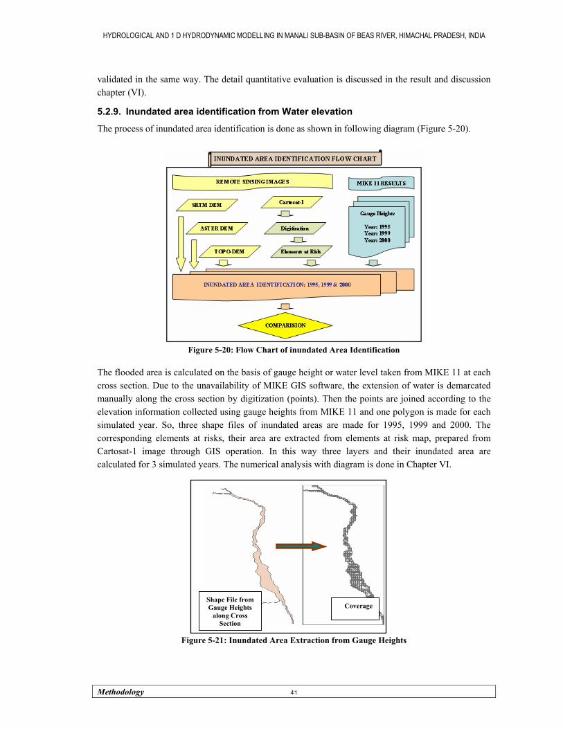
HYDROLOGICAL AND 1 D HYDRODYNAMIC MODELLING IN MANALI SUB-BASIN OF BEAS RIVER, HIMACHAL PRADESH, INDIA
Methodology 41
validated in the same way. The detail quantitative evaluation is discussed in the result and discussion chapter (VI).
5.2.9. Inundated area identification from Water elevation
The process of inundated area identification is done as shown in following diagram (Figure 5-20).
Figure 5-20: Flow Chart of inundated Area Identification
The flooded area is calculated on the basis of gauge height or water level taken from MIKE 11 at each cross section. Due to the unavailability of MIKE GIS software, the extension of water is demarcated manually along the cross section by digitization (points). Then the points are joined according to the elevation information collected using gauge heights from MIKE 11 and one polygon is made for each simulated year. So, three shape files of inundated areas are made for 1995, 1999 and 2000. The corresponding elements at risks, their area are extracted from elements at risk map, prepared from Cartosat-1 image through GIS operation. In this way three layers and their inundated area are calculated for 3 simulated years. The numerical analysis with diagram is done in Chapter VI.
Figure 5-21: Inundated Area Extraction from Gauge Heights
Shape File from Gauge Heights
along Cross Section
Coverage
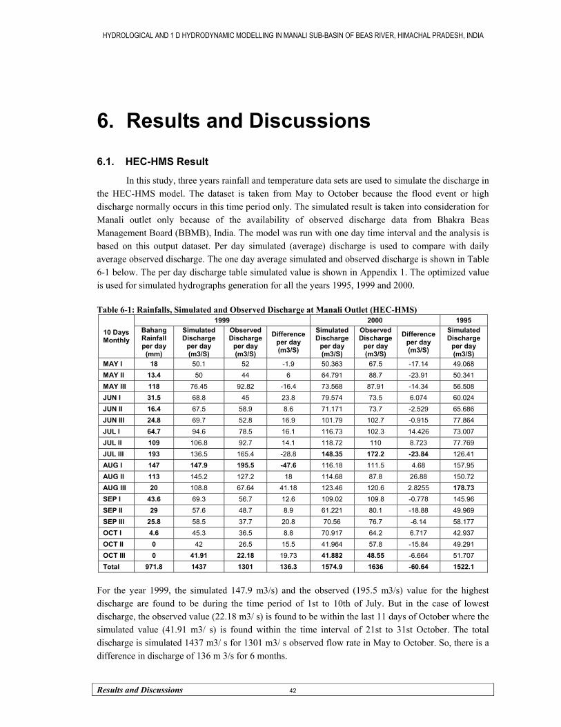
HYDROLOGICAL AND 1 D HYDRODYNAMIC MODELLING IN MANALI SUB-BASIN OF BEAS RIVER, HIMACHAL PRADESH, INDIA
Results and Discussions 42
6. Results and Discussions
6.1. HEC-HMS Result
In this study, three years rainfall and temperature data sets are used to simulate the discharge in the HEC-HMS model. The dataset is taken from May to October because the flood event or high discharge normally occurs in this time period only. The simulated result is taken into consideration for Manali outlet only because of the availability of observed discharge data from Bhakra Beas Management Board (BBMB), India. The model was run with one day time interval and the analysis is based on this output dataset. Per day simulated (average) discharge is used to compare with daily average observed discharge. The one day average simulated and observed discharge is shown in Table 6-1 below. The per day discharge table simulated value is shown in Appendix 1. The optimized value is used for simulated hydrographs generation for all the years 1995, 1999 and 2000. Table 6-1: Rainfalls, Simulated and Observed Discharge at Manali Outlet (HEC-HMS)
1999 2000 1995
10 Days Monthly
Bahang Rainfall per day (mm)
Simulated Discharge
per day (m3/S)
Observed Discharge
per day (m3/S)
Difference per day (m3/S)
Simulated Discharge
per day (m3/S)
Observed Discharge
per day (m3/S)
Difference per day (m3/S)
Simulated Discharge
per day (m3/S)
MAY I 18 50.1 52 -1.9 50.363 67.5 -17.14 49.068 MAY II 13.4 50 44 6 64.791 88.7 -23.91 50.341 MAY III 118 76.45 92.82 -16.4 73.568 87.91 -14.34 56.508 JUN I 31.5 68.8 45 23.8 79.574 73.5 6.074 60.024 JUN II 16.4 67.5 58.9 8.6 71.171 73.7 -2.529 65.686 JUN III 24.8 69.7 52.8 16.9 101.79 102.7 -0.915 77.864 JUL I 64.7 94.6 78.5 16.1 116.73 102.3 14.426 73.007 JUL II 109 106.8 92.7 14.1 118.72 110 8.723 77.769 JUL III 193 136.5 165.4 -28.8 148.35 172.2 -23.84 126.41 AUG I 147 147.9 195.5 -47.6 116.18 111.5 4.68 157.95 AUG II 113 145.2 127.2 18 114.68 87.8 26.88 150.72 AUG III 20 108.8 67.64 41.18 123.46 120.6 2.8255 178.73 SEP I 43.6 69.3 56.7 12.6 109.02 109.8 -0.778 145.96 SEP II 29 57.6 48.7 8.9 61.221 80.1 -18.88 49.969 SEP III 25.8 58.5 37.7 20.8 70.56 76.7 -6.14 58.177 OCT I 4.6 45.3 36.5 8.8 70.917 64.2 6.717 42.937 OCT II 0 42 26.5 15.5 41.964 57.8 -15.84 49.291 OCT III 0 41.91 22.18 19.73 41.882 48.55 -6.664 51.707 Total 971.8 1437 1301 136.3 1574.9 1636 -60.64 1522.1
For the year 1999, the simulated 147.9 m3/s) and the observed (195.5 m3/s) value for the highest discharge are found to be during the time period of 1st to 10th of July. But in the case of lowest discharge, the observed value (22.18 m3/ s) is found to be within the last 11 days of October where the simulated value (41.91 m3/ s) is found within the time interval of 21st to 31st October. The total discharge is simulated 1437 m3/ s for 1301 m3/ s observed flow rate in May to October. So, there is a difference in discharge of 136 m 3/s for 6 months.
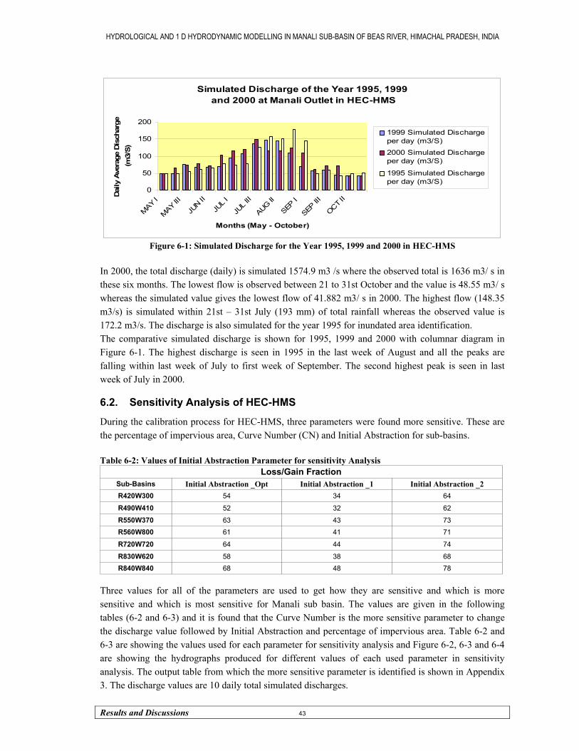
HYDROLOGICAL AND 1 D HYDRODYNAMIC MODELLING IN MANALI SUB-BASIN OF BEAS RIVER, HIMACHAL PRADESH, INDIA
Results and Discussions 43
Simulated Discharge of the Year 1995, 1999 and 2000 at Manali Outlet in HEC-HMS
0
50
100
150
200
MAY I
MAY III
JUN II
JUL I
JUL I
II
AUG II
SEP I
SEP III
OCT II
Months (May - October)
Dai
ly A
vera
ge D
isch
arge
(m
3/S
)1999 Simulated Dischargeper day (m3/S)
2000 Simulated Dischargeper day (m3/S)
1995 Simulated Dischargeper day (m3/S)
Figure 6-1: Simulated Discharge for the Year 1995, 1999 and 2000 in HEC-HMS In 2000, the total discharge (daily) is simulated 1574.9 m3 /s where the observed total is 1636 m3/ s in these six months. The lowest flow is observed between 21 to 31st October and the value is 48.55 m3/ s whereas the simulated value gives the lowest flow of 41.882 m3/ s in 2000. The highest flow (148.35 m3/s) is simulated within 21st – 31st July (193 mm) of total rainfall whereas the observed value is 172.2 m3/s. The discharge is also simulated for the year 1995 for inundated area identification. The comparative simulated discharge is shown for 1995, 1999 and 2000 with columnar diagram in Figure 6-1. The highest discharge is seen in 1995 in the last week of August and all the peaks are falling within last week of July to first week of September. The second highest peak is seen in last week of July in 2000.
6.2. Sensitivity Analysis of HEC-HMS
During the calibration process for HEC-HMS, three parameters were found more sensitive. These are the percentage of impervious area, Curve Number (CN) and Initial Abstraction for sub-basins. Table 6-2: Values of Initial Abstraction Parameter for sensitivity Analysis
Loss/Gain Fraction Sub-Basins Initial Abstraction _Opt Initial Abstraction _1 Initial Abstraction _2 R420W300 54 34 64
R490W410 52 32 62
R550W370 63 43 73 R560W800 61 41 71
R720W720 64 44 74
R830W620 58 38 68 R840W840 68 48 78
Three values for all of the parameters are used to get how they are sensitive and which is more sensitive and which is most sensitive for Manali sub basin. The values are given in the following tables (6-2 and 6-3) and it is found that the Curve Number is the more sensitive parameter to change the discharge value followed by Initial Abstraction and percentage of impervious area. Table 6-2 and 6-3 are showing the values used for each parameter for sensitivity analysis and Figure 6-2, 6-3 and 6-4 are showing the hydrographs produced for different values of each used parameter in sensitivity analysis. The output table from which the more sensitive parameter is identified is shown in Appendix 3. The discharge values are 10 daily total simulated discharges.

HYDROLOGICAL AND 1 D HYDRODYNAMIC MODELLING IN MANALI SUB-BASIN OF BEAS RIVER, HIMACHAL PRADESH, INDIA
Results and Discussions 44
Sensitivity with Initial Abstraction
1563.281894
0
500
1000
1500
2000
MAY I
MAY II
MAY IIIJU
N I
JUN II
JUN III
JUL I
JUL I
I
JUL I
II
AUG I
AUG II
AUG III
SEP I
SEP II
SEP III
OCT I
OCT II
OCT III
Month - 10 Daily (May - October)
Dis
char
ge (m
3/S
)
IA_1 IA_Opt IA_2 Observed_Value
Figure 6-2: Changes in Discharge due to Change in Loss/Gain Fraction at Manali Outlet, 2000 Table 6-3: The Impervious area (%) and CN Values Used for Sensitivity Analysis
Sub-Basins Impervious %_Opt Impervious %_1 Impervious %_2 CN _Opt CN_1 CN_2
R420W300 12.66 25.32 6.33 88 98 68
R490W410 8.97 17.94 4.485 81 91 61
R550W370 6.61 13.22 3.305 85 95 65
R560W800 2.21 4.43 1.105 88 98 68
R720W720 1.53 3.06 0.765 85 95 65
R830W620 2.06 4.12 1.03 74 84 54
R840W840 14.11 28.22 7.055 87 97 67
The optimized (Opt) values for each sub-basin are fixed on the basis of best possible result, shown in the first column of Table 6-3 and first and fifth column of Table 6-4 for respective and then other used value (1 an 2) are shown in the same tables.
Sensitivity with Impervious Area
1563.241894
0
500
1000
1500
2000
MAY I
MAY II
MAY IIIJU
N I
JUN II
JUN III
JUL I
JUL I
I
JUL I
II
AUG I
AUG II
AUG III
SEP I
SEP II
SEP III
OCT I
OCT II
OCT III
Month - 10 Daily (May - October)
Dis
char
ge (m
3/S
)
Imp_1 Imp_Opt Imp_2 Observed_Value
Figure 6-3: Changes in Discharge due to Change in % of Impervious Area at Manali Outlet, 2000
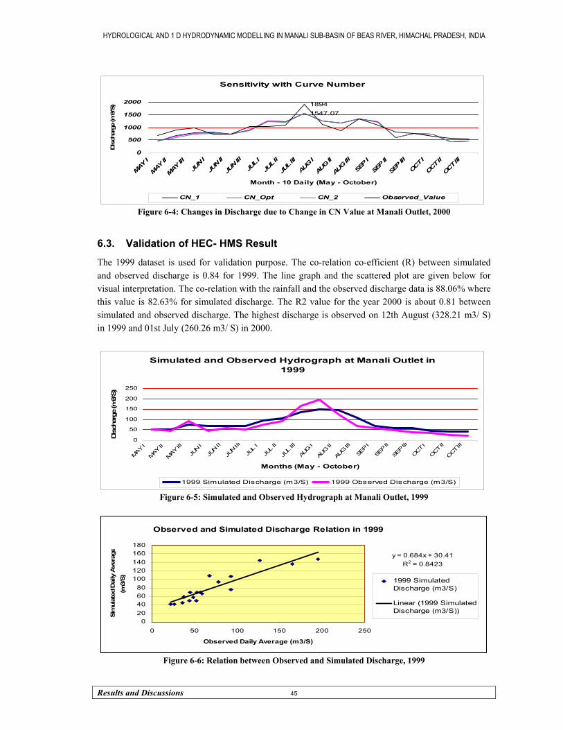
HYDROLOGICAL AND 1 D HYDRODYNAMIC MODELLING IN MANALI SUB-BASIN OF BEAS RIVER, HIMACHAL PRADESH, INDIA
Results and Discussions 45
Sensitivity with Curve Number
1547.071894
0
500
1000
1500
2000
MAY
I
MAY
II
MAY
III
JUN
I
JUN
II
JUN
III
JUL I
JUL II
JUL III
AUG I
AUG II
AUG II
I
SEP
I
SEP
II
SEP
III
OCT I
OCT II
OCT III
Month - 10 Daily (May - October)
Dis
char
ge (m
3/S)
CN_1 CN_Opt CN_2 Observed_Value
Figure 6-4: Changes in Discharge due to Change in CN Value at Manali Outlet, 2000
6.3. Validation of HEC- HMS Result
The 1999 dataset is used for validation purpose. The co-relation co-efficient (R) between simulated and observed discharge is 0.84 for 1999. The line graph and the scattered plot are given below for visual interpretation. The co-relation with the rainfall and the observed discharge data is 88.06% where this value is 82.63% for simulated discharge. The R2 value for the year 2000 is about 0.81 between simulated and observed discharge. The highest discharge is observed on 12th August (328.21 m3/ S) in 1999 and 01st July (260.26 m3/ S) in 2000.
Simulated and Observed Hydrograph at Manali Outlet in 1999
0
50
100
150
200
250
MAY
I
MAY
II
MAY
III
JUN
I
JUN
II
JUN
III
JUL I
JUL II
JUL III
AUG I
AUG II
AUG III
SEP I
SEP II
SEP III
OCT
I
OCT
II
OCT
III
Months (May - October)
Dis
char
ge (m
3/S)
1999 Simulated Discharge (m3/S) 1999 Observed Discharge (m3/S)
Figure 6-5: Simulated and Observed Hydrograph at Manali Outlet, 1999
Observed and Simulated Discharge Relation in 1999
y = 0.684x + 30.41R2 = 0.8423
020406080
100120140160180
0 50 100 150 200 250
Observed Daily Average (m3/S)
Sim
ulat
ed D
aily
Ave
rage
(m3/
S) 1999 SimulatedDischarge (m3/S)
Linear (1999 SimulatedDischarge (m3/S))
Figure 6-6: Relation between Observed and Simulated Discharge, 1999

HYDROLOGICAL AND 1 D HYDRODYNAMIC MODELLING IN MANALI SUB-BASIN OF BEAS RIVER, HIMACHAL PRADESH, INDIA
Results and Discussions 46
Figure 6-5 and 6-6 are showing the hydrographs and scattered plot of simulated and observed discharge for the year 1999 and Figure 6-7 and 6-8 in case 2000 for the same. There is a considerable difference in highest peak discharge between simulated and observed discharge though it is less in case of other peaks. The optimized dataset is used for simulation of all used years. There are some missing values in time series rainfall data for each used year. 2-3 days missing data can make a difference in discharge if there is any intensive precipitation amount. The result of HEC-HMS is used in MIKE 11 as input boundary parameter, so the inaccuracy or less accuracy in result affects the validation result of MIKE 11.
Simulated and Observed Hydrograph at Manali Outlet in 2000
0
50
100
150
200
MAYI
MAYII
MAYIII
JUN I JUNII
JUNIII
JUL I JULII
JULIII
AUGI
AUGII
AUGIII
SEP I SEPII
SEPIII
OCTI
OCTII
OCTIII
Months (May - October)
Sim
ulat
ed D
aily
Ave
rage
(m3/
S)
2000 Simulated Discharge (m3/S) 2000 Observed Discharge (m3/S)
Figure 6-7: Simulated and Observed Hydrograph at Manali Outlet, 2000
Observed and Simulated Discharge Relation in 2000
y = 0.9868x - 2.1717R2 = 0.8076
020406080
100120140160180
0 50 100 150 200
Observed Daily Average (m3/S)
Sim
ulat
ed D
aily
Ave
rage
(m3/
S)
2000 Simulated Discharge(m3/S)Linear (2000 SimulatedDischarge (m3/S))
Figure 6-8: Correlation between Observed and Simulated Discharge for 2000
The correlation coefficient between 1999 rainfall and simulated discharge is 0.73 where this value is 0.88 for the rainfall-observed discharge relation. The scattered plot for 1999 is shown in Appendix 2.
6.4. MIKE 11 Result
The 2000 dataset is used for calibration of the model and it is validated with 1999 dataset. Outflow hydrographs from HEC-HMS are used here as boundary parameter. The only parameter Manning’s ‘N’ value for roughness is used for sensitivity analysis with 2000 dataset. The 10 daily total discharge data is converted into daily average discharges for validation purpose. The simulated highest and lowest discharge value is 164.42m3/S is 47.2m3/ S in August I and October III time span respectively. The highest and lowest observed values are 195.5m3/S and 25.02m3/S on respective dates similar to simulated dates of 1999. The total simulated and observed discharge is 1603.9 and 1376 m3/S in 1999.

HYDROLOGICAL AND 1 D HYDRODYNAMIC MODELLING IN MANALI SUB-BASIN OF BEAS RIVER, HIMACHAL PRADESH, INDIA
Results and Discussions 47
Highest and lowest discharge is 189.4 m3/ S and 57.8 m3/ S in July III and October II time span in 2000. Simulation is also done for 1995 and it is used for inundated area identification. The detail per day discharge information table is shown in appendix 2. Table 6-4: Rainfall, Simulate and Observed Discharge at Manali Outlet (MIKE 11)
1999 2000 1995
10 Days Monthly
Bahang Daily
Rainfall (mm)
Simulated daily
Discharge (m3/S)
Observed Daily Avg. Discharge
(m3/S)
Difference (m3/S)
Simulated Daily
Discharge (m3/S)
Observed Daily Avg. Discharge
(m3/S)
Difference (m3/S)
Simulated Daily
Discharge (m3/S)
MAY I 18 51.585 52 -0.415 51.595 67.5 -15.9 50.834 MAY II 13.4 56.5 44 12.5 73.124 88.7 -15.6 56.5 MAY III 118 77.717 92.82 -15.101 92.506 96.7 -4.19 64.042 JUN I 31.5 78.221 45 33.221 90.932 73.5 17.43 68.455 JUN II 16.4 76.886 58.9 17.986 81.228 73.7 7.527 75.021 JUN III 24.8 79.345 52.8 26.545 116.66 102.7 13.96 89.034 JUL I 64.7 107.27 78.5 28.773 132.94 102.3 30.64 82.62 JUL II 109 121.43 92.7 28.726 135.26 110 25.26 88.335 JUL III 193 155.62 169.5 -13.856 186.42 189.4 -2.98 143.22 AUG I 147 164.42 195.5 -31.08 127.92 111.5 16.42 177.37 AUG II 113 160.82 127.2 33.618 125.73 87.8 37.93 168.11 AUG III 20 119.02 136 -16.965 149.59 132.7 16.89 200.12 SEP I 43.6 78.162 56.7 21.462 123.96 109.8 14.16 165.5 SEP II 29 65.293 48.7 16.593 69.48 80.1 -10.6 56.458 SEP III 25.8 66.216 37.7 28.516 80.13 76.7 3.43 66.26 OCT I 4.6 50.964 36.5 14.464 80.591 64.2 16.39 48.281 OCT II 0 47.2 26.5 20.7 47.2 57.8 -10.6 55.912 OCT III 0 47.2 25.02 22.182 51.92 53.4 -1.48 58.633 Total 971.8 1603.9 1376 227.87 1817.2 1679 138.7 1714.7
In case of 2000, highest simulated discharge (186.42 m3/ S) is almost nearer to each other and on the same time period (Jul. III) where the lowest simulated flow 47.2 m3/ S is comparatively lower than observed value by 10.6 m3/S. The gauge heights of peak discharge period are also taken for 31 cross sections for all the mentioned years. Figure 6-9 is showing the hydrographs of simulated and observed discharge for 1999 and 2000.
Simulated and Observed Discharge at Manali Outlet in 1999 and 2000
0
50
100
150
200
250
MAY I
MAY III
JUN II
JUL I
JUL III
AUG II
SEP I
SEP III
OCT II
Months (May - October)
Dai
ly D
isch
arge
(m3/
S)
1999 Simulated daily Discharge(m3/S)
1999 Observed Daily Avg.Discharge (m3/S)
2000 Simulated DailyDaiDischarge (m3/S)
2000 Observed Daily Avg.Discharge (m3/S)
Figure 6-9: Observed and Simulated Discharge for 1999 and 2000

HYDROLOGICAL AND 1 D HYDRODYNAMIC MODELLING IN MANALI SUB-BASIN OF BEAS RIVER, HIMACHAL PRADESH, INDIA
Results and Discussions 48
6.5. Sensitivity Analysis of MIKE 11
The roughness co-efficient value ‘N’ is used to observe the relationship between the roughness of channel and discharge amount for 2000 datasets. Three values 0.015, 0.45 and 0.08 are used globally for this purpose. No such change in 10 daily total discharges is found as given in the following table. Among these values, 0.045 is giving most suitable output as shown in the validation part. The values were taken globally because the channel morphology is almost similar throughout the reaches. Table 6-5: N values and discharge
Time N_0.045 N_0.08 N_0.015 2000 Observed MAY I 515.95 515.91 515.84 675
MAY II 731.24 731.27 731.37 887
MAY III 925.06 924.90 924.79 967
JUN I 909.32 909.36 909.52 735
JUN II 812.27 812.45 812.73 737
JUN III 1166.57 1166.10 1165.56 1027
JUL I 1329.37 1330.03 1330.73 1023
JUL II 1352.56 1352.87 1353.14 1100
JUL III 1864.24 1864.08 1863.69 1894
AUG I 1279.19 1279.58 1280.05 1115
AUG II 1257.28 1257.31 1257.39 878
AUG III 1495.88 1495.55 1495.25 1327
SEP I 1239.61 1240.17 1240.96 1098
SEP II 694.79 694.57 694.33 801
SEP III 801.30 801.63 802.091 767
OCT I 805.91 806.00 806.157 642
OCT II 472 472 472 578
OCT III 519.2 519.2 519.2 534
Variability in Discharge for Different Manning's ‘N’ at Manali Outlet, 2000
0
500
1000
1500
2000
MAY
I
MAY
III
JUN II
JUL I
JUL III
AUG II
SEP I
SEP III
OCT II
Month - 10 Daily (May - October)
Dis
char
ge (m
3/S)
N_0.33N_0.08N_0.0152000 Observed
Figure 6-10: Graphs Showing Discharge amounts for Different N values and Observed Discharge
This is happened probably due to the sudden change in width because of some mid-channel bar and convergence of alluvial fan, structured controlled meandering, break of slope and effected velocity change in the channel. The energy is used for concave-bank side erosion at the meanders and as a result velocity decreases. The velocity is high where alluvial fans make the channel congested (contraction) and it is less where it flows in a wide channel (expansion) after the narrow congested stretch and flows over a deposited bar covered with orchards. The kinetic energy (momentum) is
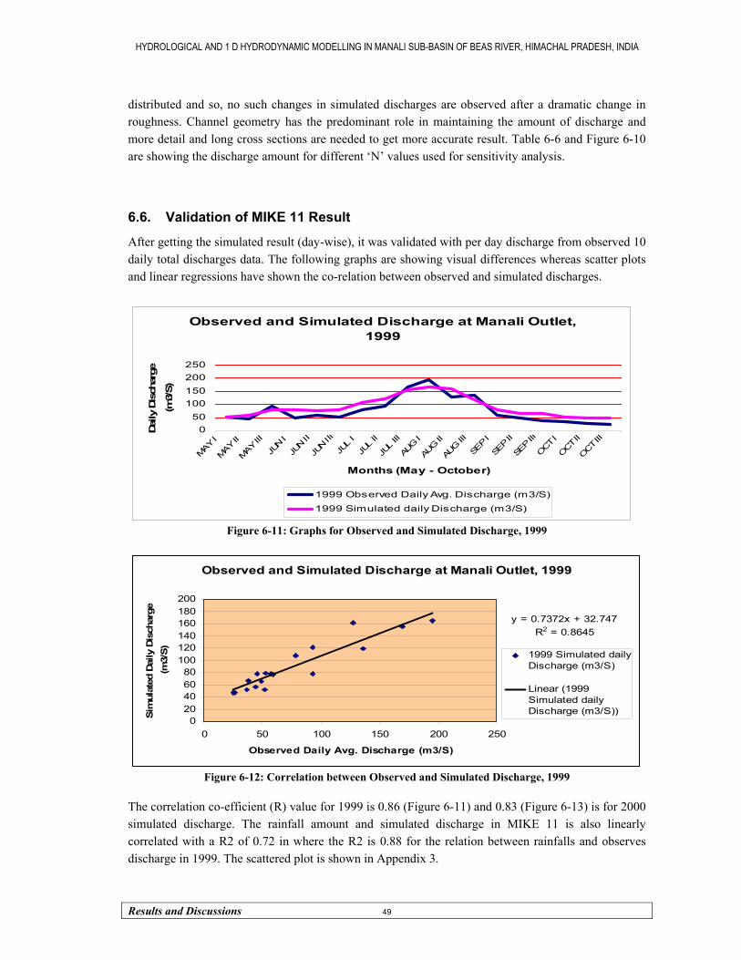
HYDROLOGICAL AND 1 D HYDRODYNAMIC MODELLING IN MANALI SUB-BASIN OF BEAS RIVER, HIMACHAL PRADESH, INDIA
Results and Discussions 49
distributed and so, no such changes in simulated discharges are observed after a dramatic change in roughness. Channel geometry has the predominant role in maintaining the amount of discharge and more detail and long cross sections are needed to get more accurate result. Table 6-6 and Figure 6-10 are showing the discharge amount for different ‘N’ values used for sensitivity analysis.
6.6. Validation of MIKE 11 Result
After getting the simulated result (day-wise), it was validated with per day discharge from observed 10 daily total discharges data. The following graphs are showing visual differences whereas scatter plots and linear regressions have shown the co-relation between observed and simulated discharges.
Observed and Simulated Discharge at Manali Outlet, 1999
050
100150200250
MAY I
MAY II
MAY
III
JUN I
JUN II
JUN II
I
JUL I
JUL II
JUL III
AUG I
AUG II
AUG III
SEP I
SEP II
SEP III
OCT I
OCT
II
OCT
III
Months (May - October)
Dai
ly D
isch
arge
(m3/
S)
1999 Observed Daily Avg. Discharge (m3/S)
1999 Simulated daily Discharge (m3/S)
Figure 6-11: Graphs for Observed and Simulated Discharge, 1999
Observed and Simulated Discharge at Manali Outlet, 1999
y = 0.7372x + 32.747R2 = 0.8645
020406080
100120140160180200
0 50 100 150 200 250
Observed Daily Avg. Discharge (m3/S)
Sim
ulat
ed D
aily
Dis
char
ge
(m3/
S) 1999 Simulated dailyDischarge (m3/S)
Linear (1999Simulated dailyDischarge (m3/S))
Figure 6-12: Correlation between Observed and Simulated Discharge, 1999
The correlation co-efficient (R) value for 1999 is 0.86 (Figure 6-11) and 0.83 (Figure 6-13) is for 2000 simulated discharge. The rainfall amount and simulated discharge in MIKE 11 is also linearly correlated with a R2 of 0.72 in where the R2 is 0.88 for the relation between rainfalls and observes discharge in 1999. The scattered plot is shown in Appendix 3.

HYDROLOGICAL AND 1 D HYDRODYNAMIC MODELLING IN MANALI SUB-BASIN OF BEAS RIVER, HIMACHAL PRADESH, INDIA
Results and Discussions 50
Observed and Simulated Discharge at Manali Outlet, 2000
0
50
100
150
200
MAYI
MAYII
MAYIII
JUNI
JUNII
JUNIII
JULI
JULII
JULIII
AUGI
AUGII
AUGIII
SEPI
SEPII
SEPIII
OCTI
OCTII
OCTIII
Months (May - October)
Dai
ly D
isch
arge
(m3/
S)
2000 Simulated Daily DaiDischarge (m3/S) 2000 Observed Daily Avg. Discharge (m3/S)
Figure 6-13: Graphs for Observed and Simulated Discharge, 2000
Observed and Simulated Discharge at Manali Outlet, 2000
y = 0.7653x + 15.993R2 = 0.8333
020406080
100120140160180200
0 50 100 150 200
Observed Daily Avg. Discharge (m3/S)
Obs
erve
d Da
ily D
isch
arge
(m3/
S) 2000 Observed Daily Avg.
Discharge (m3/S)
Linear (2000 ObservedDaily Avg. Discharge(m3/S))
Figure 6-14: Correlation between Observed and Simulated Discharge, 2000
6.7. Inundated area and damage area identification
The flood maps are generated from highest water level at cross sections along the reaches and then the flooded or inundated area is calculated from Cartosat 1 image as mentioned in the methodology chapter. Mainly the water occupied channel area is demarcated as areal extent is less (up to about 170m3/S daily) in 1999 and in 2000. Because of heavy rainfall in 1995, river side area (left bank) like SASE campus, BRO campus and adjoining roads etc. were inundated with a few (0.1 – 0.4 m) meter of water level depending upon the elevation of motioned places. The highest gauge height is taken for water occupied area identification and these are 4th September, 12th August and 1st July for the years 1995, 1999 and 2000 respectively. Though flood events are not frequent phenomena here, but a sudden cloud burst and resultant rainfall inundate the low areas. The water level for each year at all the cross sections is given in Appendix 3. Table 6-6: Affected Area and Elements at Risk from Cartosat 1 Image in 1995, 1999 and 2000
Elements at Risks Water Occupied Area(Km2) 1995
Water Occupied Area(Km2) 1999
Water Occupied Area(Km2) 2000
Bushes & Trees 0.09 0.09 0.09 Orchards 0.03 0.03 0.03 Settlement 0.24 0 0
River Channel 1.03 1.03 1.0 Total area 1.39 1.15 1.12
Road Length 938.42 m 0 0
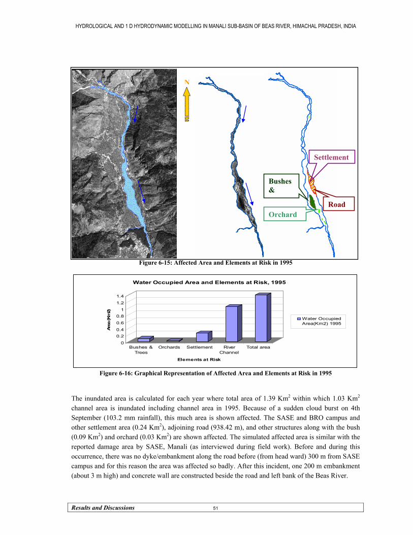
HYDROLOGICAL AND 1 D HYDRODYNAMIC MODELLING IN MANALI SUB-BASIN OF BEAS RIVER, HIMACHAL PRADESH, INDIA
Results and Discussions 51
Figure 6-15: Affected Area and Elements at Risk in 1995
0
0.20.4
0.6
0.81
1.2
1.4
Are
a (K
m2)
Bushes &Trees
Orchards Settlement RiverChannel
Total area
Elements at Risk
Water Occupied Area and Elements at Risk, 1995
Water OccupiedArea(Km2) 1995
Figure 6-16: Graphical Representation of Affected Area and Elements at Risk in 1995
The inundated area is calculated for each year where total area of 1.39 Km2 within which 1.03 Km2
channel area is inundated including channel area in 1995. Because of a sudden cloud burst on 4th September (103.2 mm rainfall), this much area is shown affected. The SASE and BRO campus and other settlement area (0.24 Km2), adjoining road (938.42 m), and other structures along with the bush (0.09 Km2) and orchard (0.03 Km2) are shown affected. The simulated affected area is similar with the reported damage area by SASE, Manali (as interviewed during field work). Before and during this occurrence, there was no dyke/embankment along the road before (from head ward) 300 m from SASE campus and for this reason the area was affected so badly. After this incident, one 200 m embankment (about 3 m high) and concrete wall are constructed beside the road and left bank of the Beas River.
N
Settlement
Bushes &
Orchard Road

HYDROLOGICAL AND 1 D HYDRODYNAMIC MODELLING IN MANALI SUB-BASIN OF BEAS RIVER, HIMACHAL PRADESH, INDIA
Results and Discussions 52
Figure 6-17: Channel Area Occupied by Water in 1999 and 2000 It is clear from the above Table 6-6 that, the water occupied area is only channel area in 1999 and 2000. The affected elements are only bushes, trees and orchards which are situated on the deposited bars along the channel. As the bars are 1-2.5 m high from the highest peak is simulated, these elements are partially affected in 1999 and 2000. Because of the construction of an embankment after 1995, the effect of high water level became less. The comparative areas of different elements at risk are shown in following Figure 6-18. For more details and diagrammatic view, see Figure 6-15 to 6-18.
0
0.2
0.4
0.6
0.8
1
1.2
1.4
Are
a (K
m2)
Bushes &Trees
Orchards Settlement RiverChannel
Total area
Elements at Risk
Water Occupied Area and Elements at Risk in 1995, 1999 and 2000
Water Occupied Area(Km2)1995Water Occupied Area(Km2)1999Water Occupied Area(Km2)2000
Figure 6-18: Comparative Graphical Representation of Inundated Area and Elements at Risks
N N

HYDROLOGICAL AND 1 D HYDRODYNAMIC MODELLING IN MANALI SUB-BASIN OF BEAS RIVER, HIMACHAL PRADESH, INDIA
Conclusion and Recommendations 53
7. Conclusion and Recommendations
Based on the research objectives and questions, the achieved conclusions and recommendations for probable future works are given in this chapter.
7.1. Conclusions
The main objective of this study is calibration and validation of HEC-HMS and MIKE 11 models and inundated area identification on DEMs using gauge heights obtained from MIKE 11.
The specific objectives are –
• Evaluate the input parameters for HEC-HMS and MIKE 11 model and flood flow simulation at the observed cross-section.
• Different inundated area calculation due to the change in water levels for three historical rainfall dataset.
Three Research questions were formulated to reach the objective mentioned above. The first research question draws attention towards the required parameters for both the hydrologic and hydraulic models. The used parameters for the models, their derivation process and use in the models are given and discussed in previous sections. The basin, hydrological and hydraulic parameters for HEC-HMS are extracted and prepared in GIS layers from ASTER DEM, field survey, observed data, maps and literatures. The final optimised values used in this study are given in Database and Materials chapter (Chapter III, Table 4.4 and Appendix 2) and Methodology chapter (Chapter IV, Table 5.2 to 5.9). The sensitivity analysis is also done to identify the most sensitive parameters in this area of study. The most sensitive parameter for HEC-HMS model is Curve Number (CN) followed by Initial Abstraction of the sub-basins among three more sensitive parameters selected for sensitivity analysis. The other one is percentage of impervious area. The output results for sensitive parameters as seen in HEC-HMS are shown in Appendix 3. Manning’s roughness co-efficient (N) is the only parameter, tested for sensitivity analysis in MIKE 11 and global value of 0.045 is used for simulation. The second research question highlights the accuracy of model results for both the model. The HEC-HMS model is used to generate the hydrographs for input boundary locations in MIKE 11. The simulated values for 1999 and 2000 ate validated with R 2 of 0.82 and 0.83 respectively. To calculate the accuracy of simulated discharge with observed dataset, the optimized dataset are used for 1999 and 2000 in MIKE 11. The highest difference in peak discharge in 1999 is about 31 m 3/s where simulated and observed discharges are 164 m 3/s and 195 m 3/s and it gives a linear correlation value(R 2) of 0.83. Similarly, the simulated, observed and the difference between two are 186 m3/s, 189 m 3/s and 3 m 3/s respectively with an R2 of 0.83. The simulated results are shown in the Table 6-1 and 6-4 for HEC-HMS and MIKE 11 respectively.
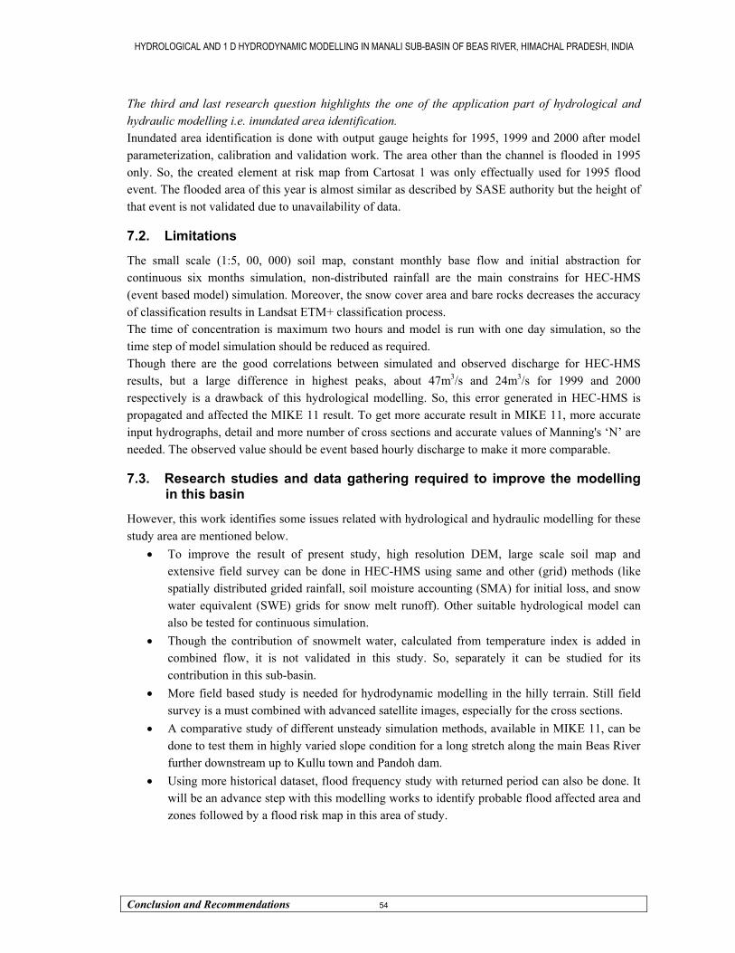
HYDROLOGICAL AND 1 D HYDRODYNAMIC MODELLING IN MANALI SUB-BASIN OF BEAS RIVER, HIMACHAL PRADESH, INDIA
Conclusion and Recommendations 54
The third and last research question highlights the one of the application part of hydrological and hydraulic modelling i.e. inundated area identification. Inundated area identification is done with output gauge heights for 1995, 1999 and 2000 after model parameterization, calibration and validation work. The area other than the channel is flooded in 1995 only. So, the created element at risk map from Cartosat 1 was only effectually used for 1995 flood event. The flooded area of this year is almost similar as described by SASE authority but the height of that event is not validated due to unavailability of data.
7.2. Limitations
The small scale (1:5, 00, 000) soil map, constant monthly base flow and initial abstraction for continuous six months simulation, non-distributed rainfall are the main constrains for HEC-HMS (event based model) simulation. Moreover, the snow cover area and bare rocks decreases the accuracy of classification results in Landsat ETM+ classification process. The time of concentration is maximum two hours and model is run with one day simulation, so the time step of model simulation should be reduced as required. Though there are the good correlations between simulated and observed discharge for HEC-HMS results, but a large difference in highest peaks, about 47m3/s and 24m3/s for 1999 and 2000 respectively is a drawback of this hydrological modelling. So, this error generated in HEC-HMS is propagated and affected the MIKE 11 result. To get more accurate result in MIKE 11, more accurate input hydrographs, detail and more number of cross sections and accurate values of Manning's ‘N’ are needed. The observed value should be event based hourly discharge to make it more comparable.
7.3. Research studies and data gathering required to improve the modelling in this basin
However, this work identifies some issues related with hydrological and hydraulic modelling for these study area are mentioned below.
• To improve the result of present study, high resolution DEM, large scale soil map and extensive field survey can be done in HEC-HMS using same and other (grid) methods (like spatially distributed grided rainfall, soil moisture accounting (SMA) for initial loss, and snow water equivalent (SWE) grids for snow melt runoff). Other suitable hydrological model can also be tested for continuous simulation.
• Though the contribution of snowmelt water, calculated from temperature index is added in combined flow, it is not validated in this study. So, separately it can be studied for its contribution in this sub-basin.
• More field based study is needed for hydrodynamic modelling in the hilly terrain. Still field survey is a must combined with advanced satellite images, especially for the cross sections.
• A comparative study of different unsteady simulation methods, available in MIKE 11, can be done to test them in highly varied slope condition for a long stretch along the main Beas River further downstream up to Kullu town and Pandoh dam.
• Using more historical dataset, flood frequency study with returned period can also be done. It will be an advance step with this modelling works to identify probable flood affected area and zones followed by a flood risk map in this area of study.
HYDROLOGICAL AND 1 D HYDRODYNAMIC MODELLING IN MANALI SUB-BASIN OF BEAS RIVER, HIMACHAL PRADESH, INDIA
Appendices 55
8. References
Acrement, G.J. and Schneider, V.R., 1989. Guide for selecting Manning’s roughness coefficients for natural channels and floodplains. Report No. FHWA-TS-84-204. Federal Highways Administration US Department of Transportation, Washington. http://www.fhwa.dot.gov/BRIDGE/wsp2339.pdf, Accessed on 12.12.2008. Agrawal, S.K., Kharya, A.K. and Khattar, R., 2001. Flood Management in Bagmati Basin, Central
Water Commission, Bihar, India. Aronica, G., Hankin, B.G. and Beven, K.J., 1998. Uncertainty and equifinalily in calibrating
distributed roughness coefficients in a flood propagation model with limited data. Advances in Water Resources Technology, 22(4): 349-365.
Baishya, B., 2004. Hydrological modelling of Umiam catchment Meghalaya using MIKE-SHE,
(B.Tech. Thesis), IIRS, India. Bates, P.D., 2004. Remote sensing and flood inundation modeling. Hydrological Processes, 18: 2593-
2597. Bates, P.D. and De Roo, A.P.J., 2000. A Simple Raster-Based model for Flood Inundation Simulation.
Journal of Hydrology, 236: 54-77. Bethke Lynne, T.P. and Janes, G., 1997. Building Capacities for Risk Reduction, 1st Ed (DMTP, ed.). Booij, M.J., 2005. Impact of Climatic Change on River Flooding Assessed with Different Spatial
Model Resolutions. Journal of Hydrology, 303: 176-198. Chow, V.T., Maidment, D.R. and Mays, L.W., 1988. Applied Hydrology, McGraw Hill Book
Company, International Edition. . Chow, V.T., Maidment, D. R. & Mays, L.W, 1995. Handbook of Applied Hydrology. Civil
Engineering Series. Congalton, R.G., 1991. A Review of Assessing the Accuracy of Classifications of Remotely Sensed
Data. Remote Sensing and Environment, 37: 35-46. Cunge, J.A., Holly Jr., F.M. and Verwey, A., 1980. Practical Aspects of Computational River
hydraulics. Pitman, London. 420. Dhar, N.O. and Nandagiri, S., 1998. Floods in Indian Rivers and their Meteorological Aspects,
Memoir Geological Society of India, Bangalore. 1-25. DHI, 2008. Project Oriented Water Modelling –Step-by Step Training Guide, Water and Environment,
Denmark. Disaster Mitigation and Vulnerability Atlas of India, Info Charge, 1992. Dutta, D., Herath, S. and Musiake, K., 2000. Flood Inundation Simulation in a River Basin Using a
Physically Based Distributed Hydrologic Model. Journal of Hydrological Processes, John Wiley & Sons, 14 (3): 497-520.
HYDROLOGICAL AND 1 D HYDRODYNAMIC MODELLING IN MANALI SUB-BASIN OF BEAS RIVER, HIMACHAL PRADESH, INDIA
Appendices 56
EM-DAT, 2008. The International Disaster Database, URL (www.em-dat.net), Accessed on:
22.11.2008. FEMA, 2000. National Flood Insurance programme 2000, Stakeholder's Report. Fetter, C.W., 2000. Applied Hydrology, New Delhi, CBS Publishers & Distributors, Second Edition. Gardner, J.S., 2002. Natural Hazard Risk in Kullu District, Himachal Pradesh, India. The
Geographical review, 92. Granger, K. and Hayne, M., 2001. Natural Hazards and Risk they Pose to South East Queensland,
Geoscience Australia in Conjunction with the Bureau of Meteorology, Commonwealth of Australia 2001, in: Hazards and Risk Concepts (AGSO, ed.), Australia.
Hunter, N.M., Bates, P.D., Horritt, M.S. and Wilson, M.D., 2007. Simple spatially-distributed models
for predicting flood inundation: a review. Geomorphology, 990: 208-225. Husain, S., M. and Rai, N.N., 2004. One dimensional dam break flood analysis for Kameng hydro
electric project, India, Central Water Commission, Arunachal Pradesh. Jain, V. and Sinha, R., 2003. Evaluation of geomorphic control on flood hazard through Geomorphic
Instantaneous Unit Hydrograph. Current Science, 85(11): 1596 – 1600. Jaiswal, R.K., Goel, N.K., Singh, P. and Thomas, T., 2003. L-Moment Based Flood Frequency
Modeling. IE (I) Journal, 84: 6-10. Karimi, H.A. and Houston, B., 1997. Evaluating strategies for integrating environmental models with
GIS: Current trends and future needs. Computer, Environment and Urban Systems, 24: 109-122.
Karssenberg, D., 2002. The value of environmental modelling languages for building distributed
hydrological models. Hydrological Processes, 16: 2751-2766. Kent, R., 1994. Disaster Preparedness Guide, DMTP, UNDP. Kumar, V., Sing, P. and Sing, V., 2007. Snow and glacier melt contribution in the Beas River at
Pandoh Dam, Himachal Pradesh, India. Hydrological Sciences, 52(2): 376-386. Kurothe, R.S., Goel, N.K. and Mathur, B.S., 2001a. Derivation of a curve number and Kinematic-
wave based flood frequency distribution. Hydrological Sciences, 46(4): 571 – 584. Kurothe, R.S., Goel, N.K. and Mathur, B.S., 2001b. Derivation of a curve number and kinematic-wave
based flood frequency distribution. Hydrological Sciences, 46: 571-584. Mahadev, H. and Prasad, V.H., 2001. Hydrological modelling of Beas basin: IIRS ITC MSc. Thesis. Mahadev, R.H. and Prasad, V.H., 2003. Hydrological modelling of Beas basin: IIRS-AU M. Tech.
Thesis. Maidment, D.R., 1993. GIS and hydrological modelling. In M. F. Goodchild, B. Parks, & L. Steyaert,
Environmental Modelling with GIS New York, USA. 147-167. Mehta, P.K., 1976. Structural and metamorphic history of the crystalline rocks of Kulu Valley,
Himachal Pradesh, in relation to tectonics of the Himalaya. Accad. Naz. Lincei, Atti Convegni Lincei,Vol. 21, pp. 215–244.
HYDROLOGICAL AND 1 D HYDRODYNAMIC MODELLING IN MANALI SUB-BASIN OF BEAS RIVER, HIMACHAL PRADESH, INDIA
Appendices 57
Mohapatra, P.K. and Sing, R.D., 2003. Flood Management in India. Natural Hazards, 28: 131 – 143. Pappenberger, F., Beven, K., Horritt, M. and Blazkova, S., 2005. Uncertainty in the calibration of
effective roughness parameters in HEC-RAS using inundation and downstream level observations. Journal of Hydrology, 302: 46-69.
Pappenberger, F., Beven, K.J., Ratto, M. and Matgen, P., 2008. Multi-Method Global Sensitivity
Analysis of Flood Inundation Models. Advance in Water Resources, 31: 1-14. Parasuraman, S. and Unnikrishnan P, V., 2000. India Disasters Report Towards A Policy Initiative,
OUP Publisher, India. Sah, M.P. and Mazari, R.K., 1998. Anthropogenically accelerated mass movement, Kulu Valley,
Himachal Pradesh, India. Geomorphology, 26: 123-138. Shankar, R. and Dua, K.J.S., 1978. On the existence of a tear fault along upper Beas Valley, District
Kulu, Himachal Pradesh, and its bearing on the thermal activity. Himalayan Geol, 8(1): 466–472.
Singh, R.L., 1992. ndia A Regional Geography. National Geographical Society. India, Varanasi. Subramanya, K., 1997. Engineering Hydrology, New Delhi, TataMcGraw-Hill, Second Edition. Subramanya, K., 2004. Engineering Hydrology, New Delhi, TataMcGraw-Hill, Second Edition. Thakur, P.K. and Sumangala, A., 2006. “Flood Inundation Mapping and 1-D Hydrodynamic Modeling
Using Remote Sensing and GIS Techniques”. ISPRS Orange Book Publications during ISPRS/ISRS commission IV symposium on: “Geospatial Database for Sustainable Development” at GOA from 27-30 September 2006.
US-SCS, 1986. (Soil Conservation Service), Urban Hydrology for Small Watersheds. Technical
Release 55, Springfield, VA. Van Loon, L.R. and Jakob, A., 2005. Evidence for a second transport porosity for the diffusion of
tritiated water (HTO) in a sedimentary rock (Opalinus Clay - OPA): application of through- and out-diffusion techniques. Transport in Porous Media, 61(2): 193-214.
van Westen, C.J., Soeters, R. and Sijmons, K., 2000. Digital geomorphological landslide hazard
mapping of the Alpago area, Italy. Journal of Applied Geomorphology 2., 1. Virdi, N.S., 1979. Status of the Chail Formation vis-a-vis Jutogh–Chail relationship in Himachal
Lessar Himalaya. Himalayan Geol, 9(1): 111–125. Walker, S., 1991. Keys to successful implementation of computer aided decision support systems in
water recourses management. Advances in Water Resources Technology: 467-472. Werner, M.G.F., Hunter, N.M. and Bates, P.D., 2005. Identifiably of distributed floodplain roughness
values in flood extent estimation. Journal of Hydrology, 314: 139-157. Wilson, J.P., 1996. GIS-base and land surface/subsurface modelling: new potential for new model?,
International conference on GIS and environmental modelling, Santa Fe, NM, USA. Websites: http:\\www.tribuneindia.com/2003/20030719/himachal.htm. Accessed on 24.05.2008 http://www.world66.com/asia/southasia/himachalpradeshindia/manali/lib/climate, Accessed on 12.11.2008)
HYDROLOGICAL AND 1 D HYDRODYNAMIC MODELLING IN MANALI SUB-BASIN OF BEAS RIVER, HIMACHAL PRADESH, INDIA
Appendices 58
9. Appendices
Appendix-1: Model Theory
HEC-HMS 3.2
This rainfall-runoff model (previously HEC-1) is used here to get the rainfall excess and its routing in the channel though it has other modules for other purposes (HEC-HMS Reference Manual, 2000). For this purpose loss, transform and routing modules are used as follows:
Loss Method
SCS23 Curve Number (CN) method (1972) is used here to calculate the initial losses and rainfall excess after the precipitation event. In this method, HSG, LULC and antecedent moisture condition are taken into account with cumulative precipitation in this area. The equation is expressed below:
SIaP
IaPPe+−
−=
2)( Equation 9-1
Where, Pe is the accumulated precipitation access at time t; P is the accumulated rainfall depth at time t; Ia is the initial abstraction (loss) and S is the potential maximum retention.
Transform Method
The following dimensionless equation is used for the transformation of surface runoff to the channel:
TpACUp = Equation 9-2
Where, A is the watershed area and C is the conversion constant (2.08 in SI and 484 in FPS system). The time of peak and duration of the unit excess precipitation is related as:
lagttTp2∆
= Equation 9-3
Where, t∆ is the duration of excess precipitation; lagt is the basin lag. The lag time is estimated through calibration and this travel time is done by TR-55 method. The time of concentration is a product of time concentration of sheet, shallow concentrated and channel flow. The time of concentration equation is given below:
)()()( ChanneltcentratedShallowContSheettc TTTT ++= Equation 9-4
Routing method
Kinematic routing method is based upon ‘finite difference approximation of continuity equation and simplification of momentum equation. The upstream and watershed surface runoff are included for trapezoidal channel routing. The equations are given below:
Discharge 32
235
12149.1)(
++=
ZYWAS
nQ Equation 9-5
23 SCS – Soil Conservation Service (now Natural Resource Conservation Service), USA. N. B. For all equations and discussions, see HEC-HMS Reference Manual, 2000 & Chow et al., 1988.
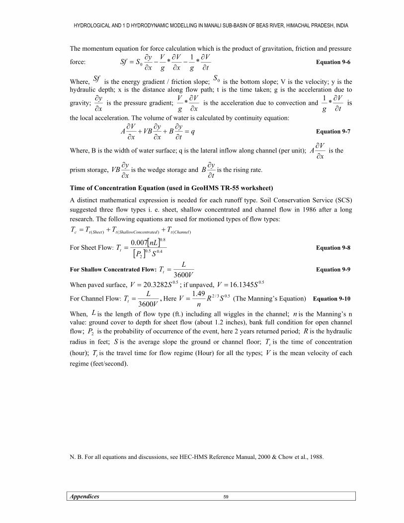
HYDROLOGICAL AND 1 D HYDRODYNAMIC MODELLING IN MANALI SUB-BASIN OF BEAS RIVER, HIMACHAL PRADESH, INDIA
Appendices 59
The momentum equation for force calculation which is the product of gravitation, friction and pressure
force: tV
gxV
gV
xySSf
∂∂
−∂∂
−∂∂
= *1*0 Equation 9-6
Where, Sf is the energy gradient / friction slope; 0S is the bottom slope; V is the velocity; y is the hydraulic depth; x is the distance along flow path; t is the time taken; g is the acceleration due to
gravity; xy∂∂ is the pressure gradient;
xV
gV
∂∂* is the acceleration due to convection and
tV
g ∂∂*1 is
the local acceleration. The volume of water is calculated by continuity equation:
qtyB
xyVB
xVA =
∂∂
+∂∂
+∂∂
Equation 9-7
Where, B is the width of water surface; q is the lateral inflow along channel (per unit); xVA∂∂ is the
prism storage, xyVB∂∂
is the wedge storage and tyB∂∂
is the rising rate.
Time of Concentration Equation (used in GeoHMS TR-55 worksheet)
A distinct mathematical expression is needed for each runoff type. Soil Conservation Service (SCS) suggested three flow types i. e. sheet, shallow concentrated and channel flow in 1986 after a long research. The following equations are used for motioned types of flow types:
)()()( ChanneltcentratedShallowContSheettc TTTT ++=
For Sheet Flow: [ ]
[ ] 4.05.02
8.0007.0SP
nLTt = Equation 9-8
For Shallow Concentrated Flow: V
LTt 3600= Equation 9-9
When paved surface, 5.03282.20 SV = ; if unpaved, 5.01345.16 SV =
For Channel Flow: V
LTt 3600= , Here 5.03/249.1 SR
nV = (The Manning’s Equation) Equation 9-10
When, L is the length of flow type (ft.) including all wiggles in the channel; n is the Manning’s n value: ground cover to depth for sheet flow (about 1.2 inches), bank full condition for open channel flow; 2P is the probability of occurrence of the event, here 2 years returned period; R is the hydraulic radius in feet; S is the average slope the ground or channel floor; cT is the time of concentration (hour); tT is the travel time for flow regime (Hour) for all the types; V is the mean velocity of each regime (feet/second). N. B. For all equations and discussions, see HEC-HMS Reference Manual, 2000 & Chow et al., 1988.
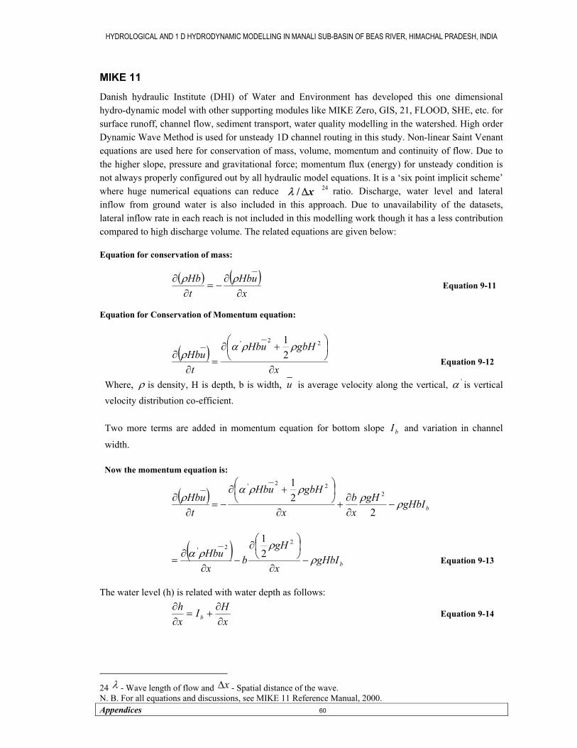
HYDROLOGICAL AND 1 D HYDRODYNAMIC MODELLING IN MANALI SUB-BASIN OF BEAS RIVER, HIMACHAL PRADESH, INDIA
Appendices 60
MIKE 11
Danish hydraulic Institute (DHI) of Water and Environment has developed this one dimensional hydro-dynamic model with other supporting modules like MIKE Zero, GIS, 21, FLOOD, SHE, etc. for surface runoff, channel flow, sediment transport, water quality modelling in the watershed. High order Dynamic Wave Method is used for unsteady 1D channel routing in this study. Non-linear Saint Venant equations are used here for conservation of mass, volume, momentum and continuity of flow. Due to the higher slope, pressure and gravitational force; momentum flux (energy) for unsteady condition is not always properly configured out by all hydraulic model equations. It is a ‘six point implicit scheme’ where huge numerical equations can reduce 24 ratio. Discharge, water level and lateral inflow from ground water is also included in this approach. Due to unavailability of the datasets, lateral inflow rate in each reach is not included in this modelling work though it has a less contribution compared to high discharge volume. The related equations are given below: Equation for conservation of mass:
( ) ( )x
uHbtHb
∂∂
−=∂
∂ ρρ Equation 9-11
Equation for Conservation of Momentum equation:
( )x
gbHuHb
tuHb
∂
+∂
=∂
∂22'
21 ρρα
ρ Equation 9-12
Where, ρ is density, H is depth, b is width, u is average velocity along the vertical, 'α is vertical velocity distribution co-efficient. Two more terms are added in momentum equation for bottom slope bI and variation in channel
width. Now the momentum equation is:
( )bgHbIgH
xb
x
gbHuHb
tuHb ρρ
ρραρ
−∂∂
+∂
+∂
−=∂
∂2
21
222'
( )bgHbI
x
gHb
xuHb ρ
ρρα
−∂
∂
−∂
∂=
22' 2
1
Equation 9-13
The water level (h) is related with water depth as follows:
xHI
xh
b ∂∂
+=∂∂
Equation 9-14
24 λ - Wave length of flow and x∆ - Spatial distance of the wave. N. B. For all equations and discussions, see MIKE 11 Reference Manual, 2000.
x∆/λ
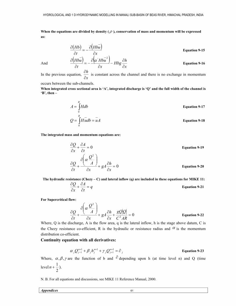
HYDROLOGICAL AND 1 D HYDRODYNAMIC MODELLING IN MANALI SUB-BASIN OF BEAS RIVER, HIMACHAL PRADESH, INDIA
Appendices 61
When the equations are divided by density ( ρ ), conservation of mass and momentum will be expressed as:
( ) ( )
xuHb
tHb
∂∂
−=∂
∂ Equation 9-15
And ( ) ( )
xhHbg
xuHb
tuHb
∂∂
−∂
∂−=
∂∂
2'α Equation 9-16
In the previous equation, xh∂∂ is constant across the channel and there is no exchange in momentum
occurs between the sub-channels. When integrated cross sectional area is ‘A’, integrated discharge is ‘Q’ and the full width of the channel is ‘B’, then –
∫=B
HdbA0
Equation 9-17
AudbuHQB
== ∫0
Equation 9-18
The integrated mass and momentum equations are:
0=∂∂
+∂∂
tA
xQ
Equation 9-19
0
2
=∂∂
+∂
∂
+∂∂
xhgA
xA
Q
tQ
α Equation 9-20
The hydraulic resistance (Chezy – C) and lateral inflow (q) are included in these equations for MIKE 11:
qtA
xQ
=∂∂
+∂∂
Equation 9-21
For Supercritical flow:
02
2
=+∂∂
+∂
∂
+∂∂
ARCQgQ
xhgA
xA
Q
tQ
α Equation 9-22
Where, Q is the discharge, A is the flow area, q is the lateral inflow, h is the stage above datum, C is the Chezy resistance co-efficient, R is the hydraulic or resistance radius and α is the momentum distribution co-efficient. Continuity equation with all derivatives:
jnjj
njj
njj QhQ ∂=++ +
+++
−11
111 γβα Equation 9-23
Where, γβα ,, are the function of b and ∂ depending upon h (at time level n) and Q (time
level21
+n ).
N. B. For all equations and discussions, see MIKE 11 Reference Manual, 2000.

HYDROLOGICAL AND 1 D HYDRODYNAMIC MODELLING IN MANALI SUB-BASIN OF BEAS RIVER, HIMACHAL PRADESH, INDIA
Appendices 62
Momentum equation using all the derivatives can be expressed as:
jnjj
njj
njj hQh ∂=++ +
+++
−11
111 γβα Equation 9-24
Where, ( ),Afj =α ( )RACxtQf n
jj ,,,,, ∆∆=β , ( )Afj =γ and
For user defined Manning’s resistance (M), the discharge is computed by the Manning’s equation:
ASMRQ 21
032
= Equation 9-25
Where M is resistance number, R is hydraulic radius, 0S is bed slope, A is cross sectional
wetted area calculated by iteration and it is placed in the cross section table of MIKE 11HD when a certain level accuracy is reached ( 310− ).
N. B. For all equations and discussions, see MIKE 11 Reference Manual, 2000.
∆∆=∂
+
++
+
−−21
1121
11 ,,,,,,,,,,,n
jnj
nj
n
jnjj QhQQhvqtxAf θα
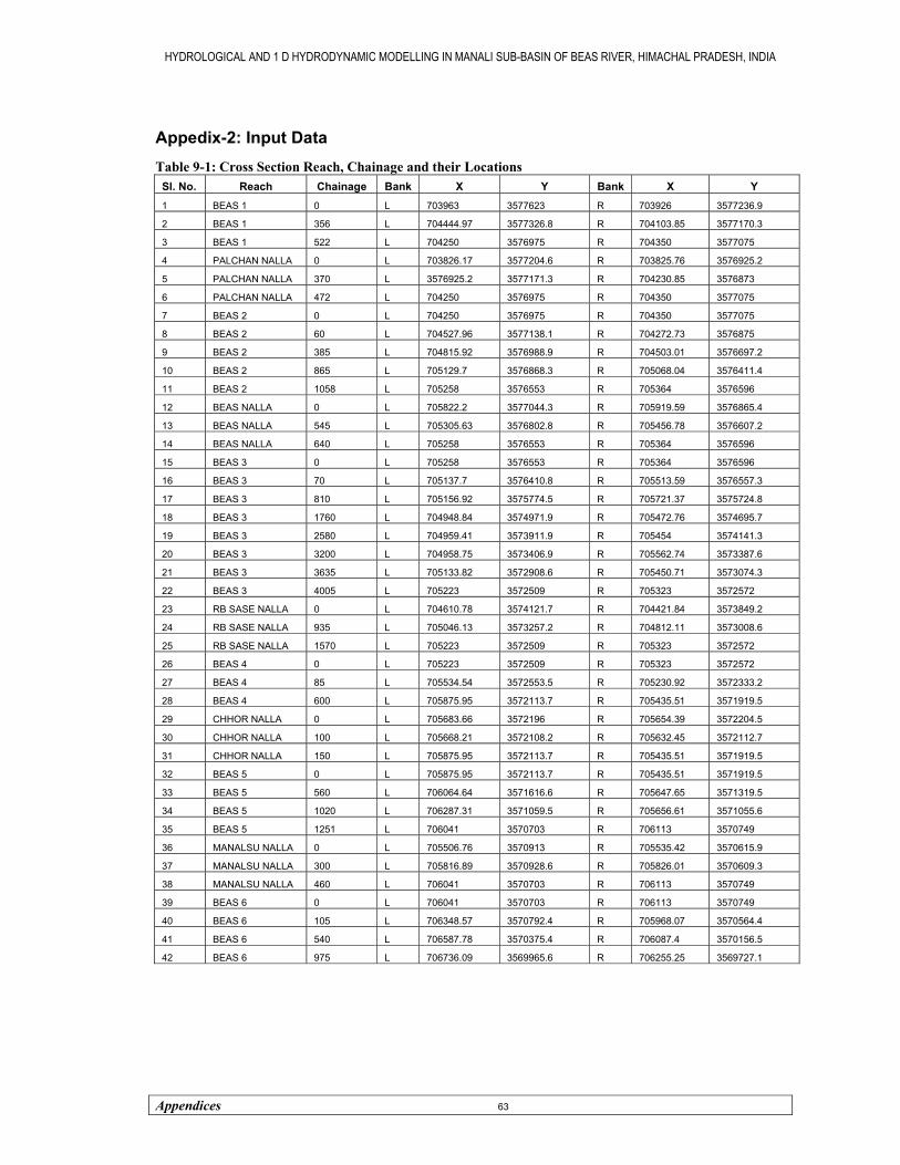
HYDROLOGICAL AND 1 D HYDRODYNAMIC MODELLING IN MANALI SUB-BASIN OF BEAS RIVER, HIMACHAL PRADESH, INDIA
Appendices 63
Appedix-2: Input Data Table 9-1: Cross Section Reach, Chainage and their Locations
Sl. No. Reach Chainage Bank X Y Bank X Y 1 BEAS 1 0 L 703963 3577623 R 703926 3577236.9
2 BEAS 1 356 L 704444.97 3577326.8 R 704103.85 3577170.3
3 BEAS 1 522 L 704250 3576975 R 704350 3577075
4 PALCHAN NALLA 0 L 703826.17 3577204.6 R 703825.76 3576925.2
5 PALCHAN NALLA 370 L 3576925.2 3577171.3 R 704230.85 3576873
6 PALCHAN NALLA 472 L 704250 3576975 R 704350 3577075
7 BEAS 2 0 L 704250 3576975 R 704350 3577075
8 BEAS 2 60 L 704527.96 3577138.1 R 704272.73 3576875
9 BEAS 2 385 L 704815.92 3576988.9 R 704503.01 3576697.2
10 BEAS 2 865 L 705129.7 3576868.3 R 705068.04 3576411.4
11 BEAS 2 1058 L 705258 3576553 R 705364 3576596
12 BEAS NALLA 0 L 705822.2 3577044.3 R 705919.59 3576865.4
13 BEAS NALLA 545 L 705305.63 3576802.8 R 705456.78 3576607.2
14 BEAS NALLA 640 L 705258 3576553 R 705364 3576596
15 BEAS 3 0 L 705258 3576553 R 705364 3576596
16 BEAS 3 70 L 705137.7 3576410.8 R 705513.59 3576557.3
17 BEAS 3 810 L 705156.92 3575774.5 R 705721.37 3575724.8
18 BEAS 3 1760 L 704948.84 3574971.9 R 705472.76 3574695.7
19 BEAS 3 2580 L 704959.41 3573911.9 R 705454 3574141.3
20 BEAS 3 3200 L 704958.75 3573406.9 R 705562.74 3573387.6
21 BEAS 3 3635 L 705133.82 3572908.6 R 705450.71 3573074.3
22 BEAS 3 4005 L 705223 3572509 R 705323 3572572
23 RB SASE NALLA 0 L 704610.78 3574121.7 R 704421.84 3573849.2
24 RB SASE NALLA 935 L 705046.13 3573257.2 R 704812.11 3573008.6
25 RB SASE NALLA 1570 L 705223 3572509 R 705323 3572572
26 BEAS 4 0 L 705223 3572509 R 705323 3572572
27 BEAS 4 85 L 705534.54 3572553.5 R 705230.92 3572333.2
28 BEAS 4 600 L 705875.95 3572113.7 R 705435.51 3571919.5
29 CHHOR NALLA 0 L 705683.66 3572196 R 705654.39 3572204.5
30 CHHOR NALLA 100 L 705668.21 3572108.2 R 705632.45 3572112.7
31 CHHOR NALLA 150 L 705875.95 3572113.7 R 705435.51 3571919.5
32 BEAS 5 0 L 705875.95 3572113.7 R 705435.51 3571919.5
33 BEAS 5 560 L 706064.64 3571616.6 R 705647.65 3571319.5
34 BEAS 5 1020 L 706287.31 3571059.5 R 705656.61 3571055.6
35 BEAS 5 1251 L 706041 3570703 R 706113 3570749
36 MANALSU NALLA 0 L 705506.76 3570913 R 705535.42 3570615.9
37 MANALSU NALLA 300 L 705816.89 3570928.6 R 705826.01 3570609.3
38 MANALSU NALLA 460 L 706041 3570703 R 706113 3570749
39 BEAS 6 0 L 706041 3570703 R 706113 3570749
40 BEAS 6 105 L 706348.57 3570792.4 R 705968.07 3570564.4
41 BEAS 6 540 L 706587.78 3570375.4 R 706087.4 3570156.5
42 BEAS 6 975 L 706736.09 3569965.6 R 706255.25 3569727.1
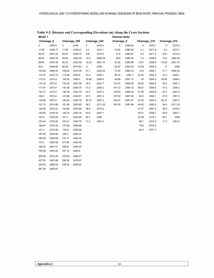
HYDROLOGICAL AND 1 D HYDRODYNAMIC MODELLING IN MANALI SUB-BASIN OF BEAS RIVER, HIMACHAL PRADESH, INDIA
Appendices 64
Table 9-2: Distance and Corresponding Elevations (m) Along the Cross Sections
Palchan Nalla Chainage_0 Chainage_370 Chainage_472
0 2386.53 0 2372.1 0 2376.4
16.65 2386.28 3.1 2371.8 2.3 2374.1
31.6 2385.87 6.3 2371.3 9.81 2370.3
38.6 2385.54 7.2 2368.8 14.5 2364.05
53.32 2384.88 8.81 2365.9 16.22 2361.15
62.97 2383.53 16.29 2364.4 17 2358
73.34 2382.32 19.5 2362.7 21.1 2354.25
85.16 2381.7 22.52 2362.3 27.4 2349.1
93.85 2381.77 24 2362.6 35.82 2348.4
101.81 2382.28 26.52 2363.6 39.3 2347.7
107.12 2384.12 36.37 2364.8 41.2 2346.2
120.63 2386.28 41.98 2364.8 44.7 2347.4
137.52 2387.08 44.5 2364.1 47.9 2351.3
163.57 2387.27 47.29 2363.4 50.31 2357.2
183.35 2387.96 49.52 2365.5 56.3 2371.25
51.87 2367.2 58.5 2379.2
55.01 2368.7 63.8 2387.1
59.38 2370.1 68.7 2390
68.1 2374.2 71.2 2391.2
79.8 2375.5
82.4 2377.3
BEAS 1 Chainage_0 Chainage_356 Chainage_522 0 2460.5 0 2440 0 2376.4
17.66 2458.77 17.66 2438.27 2.3 2374.1
36.97 2457.24 36.97 2436.74 9.81 2370.3
56.62 2450.76 56.62 2430.26 14.5 2364.05
69.84 2444.39 82.33 2423.59 16.22 2361.15
95.9 2429.84 96.26 2419.82 17 2358
103.86 2398.32 106.82 2410.39 21.1 2354.25
110.74 2374.13 113.99 2403.8 27.4 2349.1
112.91 2373.4 124.55 2384.4 35.82 2348.4
116.16 2373.4 130.04 2367.98 39.3 2347.7
117.97 2373.4 134.26 2354.79 41.2 2346.2
124.13 2373.4 136.79 2354.79 44.7 2347.4
126.3 2373.4 141.86 2352.91 47.9 2351.3
134.98 2373.4 145.24 2354.79 50.31 2357.2
137.15 2374.86 151.99 2353.85 56.3 2371.25
142.94 2376.33 153.68 2353.85 58.5 2379.2
145.84 2376.33 158.75 2354.79 63.8 2387.1
150.9 2379.26 161.7 2353.85 68.7 2390
153.44 2379.26 167.61 2354.79 71.2 2391.2
158.87 2379.26 170.99 2356.68
161.4 2379.99 179.01 2356.68
167.55 2383.66 184.5 2362.33
169.36 2383.66 197.17 2400.34
173.7 2387.85 217.85 2420.45
182.03 2441.57 236.01 2435.52
194.69 2463.55 257.12 2450.6 209.89 2472.35 276.54 2464.01
227.62 2481.88 299.34 2476.57
239.93 2485.54 324.25 2482.43
261.28 2492.87
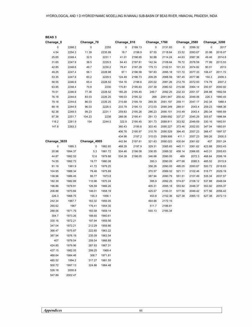
HYDROLOGICAL AND 1 D HYDRODYNAMIC MODELLING IN MANALI SUB-BASIN OF BEAS RIVER, HIMACHAL PRADESH, INDIA
Appendices 65
BEAS 3 Chanage_0 Chanage_70 Chanage_810 Chanage_1760 Chanage_2580 Chanage_3200
0 2268.2 0 2255 0 2199.13 0 2131.83 0 2099.32 0 2017
4.54 2254.3 11.39 2235.99 18.7 2198.9 67.55 2118.64 23.52 2093.67 20.98 2016.07
25.65 2249.4 32.5 2231.1 41.01 2198.65 92.88 2114.24 44.63 2087.38 49.46 2014.8
31.65 2247.9 38.5 2229.5 64.43 2197.81 142.34 2109.84 76.72 2078.59 77.99 2013.53
42.85 2248.6 49.7 2230.2 78.41 2197.29 179.13 2102.51 101.33 2074.82 90.01 2013
49.25 2247.4 56.1 2228.98 97.1 2196.58 197.83 2095.18 131.72 2077.33 106.47 2011.72
53.35 2247.9 60.2 2229.5 124.49 2196.73 209.29 2088.59 187.45 2077.96 150.3 2009.3
58.55 2246.9 65.4 2228.52 154.16 2196.6 220.02 2081.26 212.79 2072.93 174.79 2007.2
63.95 2248.4 70.8 2230 170.81 2195.63 237.39 2080.52 215.68 2064.14 200.97 2000.92
70.51 2246.9 77.36 2228.52 185.28 2195.45 249.7 2092.25 232.33 2051.57 206.88 1992.54
76.18 2244.6 83.03 2226.25 199.03 2195.32 268 2091.947 250.42 2049.06 226.3 1990.45
79.18 2244.6 86.03 2226.25 215.68 2195.19 269.35 2091.197 259.11 2047.17 242.34 1989.4
89.18 2244.9 96.03 2226.5 233.78 2195.13 272.03 2090.349 289.51 2043.4 259.23 1988.36
92.38 2249.5 99.23 2231.1 259.83 2195.26 286.23 2090.101 310.49 2043.4 280.34 1995.69
97.38 2251.7 104.23 2238 288.06 2195.41 291.13 2089.692 337.27 2045.29 305.67 1996.84
118.2 2261.9 154 2244.5 322.8 2195.45 301.73 2089.811 353.92 2049.69 330.16 1993.91
147.8 2263.3 360.43 2195.6 303.45 2090.227 373.46 2052.83 347.04 1993.91
406.76 2195.97 310.76 2090.529 394.45 2057.23 366.47 1997.57
434.98 2197.2 315.03 2089.906 411.1 2057.23 389.26 2000.5
Chanage_3635 Chanage_4005 442.94 2197.61 321.63 2090.023 430.64 2061.62 407 2001.24
0 1995.3 0 1982.65 468.28 2197.9 329.31 2085.65 445.11 2061.62 423.88 2003.43
20.98 1994.37 5.3 1981.72 504.46 2198.08 336.55 2089.32 458.14 2066.65 443.31 2005.63
44.87 1992.53 12.6 1979.88 534.38 2198.05 346.68 2090.05 469 2072.3 468.64 2006.16
74.55 1992.73 19.77 1980.08 350.3 2090.05 477.68 2085.5 485.52 2015.9
91.19 1991.9 41.72 1979.25 358.26 2090.05 495.05 2093.67 500.72 2018.83
104.95 1988.34 78.46 1975.69 370.57 2089.32 521.11 2102.46 516.77 2029.19
138.96 1986.45 95.77 1973.8 387.94 2090.79 551.51 2107.49 535.34 2037.57
182.39 1982.89 110.96 1970.24 395.9 2092.25 574.67 2108.12 537.88 2048.04
196.86 1978.91 126.59 1966.26 405.31 2095.18 553.92 2048.37 553.92 2055.37
206.88 1970.84 146.01 1958.19 425.57 2100.31 577.56 2049.42 577.56 2056.42
226.3 1968.75 155.3 1956.1 453.8 2152.36 627.38 2065.13 627.38 2072.13
242.34 1967.7 163.32 1955.05 464.66 2172.15
265.62 1967 176.41 1954.35 511.7 2186.81
288.06 1971.79 183.58 1959.14 555.13 2185.34
304.7 1973.26 188.65 1960.61
330.16 1972.21 197.94 1959.56
347.04 1972.21 212.29 1959.86
366.47 1975.87 222.85 1963.22
387.94 1976.19 235.09 1963.54
407 1979.54 259.54 1966.89
424.85 1979.96 287.93 1967.31
437.15 1982.05 299.25 1969.4
468.64 1984.46 306.7 1971.81
485.52 1994.2 317.27 1981.55
500.72 1997.13 324.86 1984.48
526.18 2000.8
547.89 2002.47
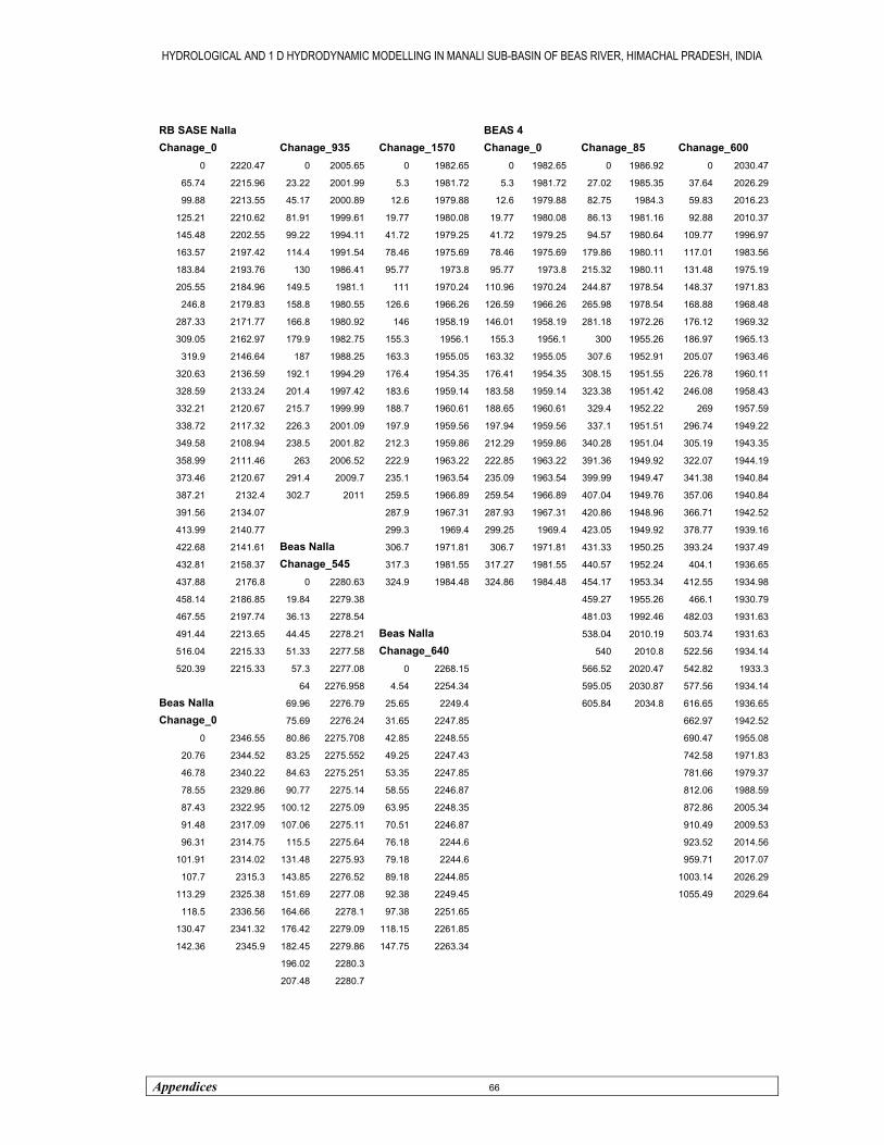
HYDROLOGICAL AND 1 D HYDRODYNAMIC MODELLING IN MANALI SUB-BASIN OF BEAS RIVER, HIMACHAL PRADESH, INDIA
Appendices 66
RB SASE Nalla BEAS 4 Chanage_0 Chanage_935 Chanage_1570 Chanage_0 Chanage_85 Chanage_600
0 2220.47 0 2005.65 0 1982.65 0 1982.65 0 1986.92 0 2030.47
65.74 2215.96 23.22 2001.99 5.3 1981.72 5.3 1981.72 27.02 1985.35 37.64 2026.29
99.88 2213.55 45.17 2000.89 12.6 1979.88 12.6 1979.88 82.75 1984.3 59.83 2016.23
125.21 2210.62 81.91 1999.61 19.77 1980.08 19.77 1980.08 86.13 1981.16 92.88 2010.37
145.48 2202.55 99.22 1994.11 41.72 1979.25 41.72 1979.25 94.57 1980.64 109.77 1996.97
163.57 2197.42 114.4 1991.54 78.46 1975.69 78.46 1975.69 179.86 1980.11 117.01 1983.56
183.84 2193.76 130 1986.41 95.77 1973.8 95.77 1973.8 215.32 1980.11 131.48 1975.19
205.55 2184.96 149.5 1981.1 111 1970.24 110.96 1970.24 244.87 1978.54 148.37 1971.83
246.8 2179.83 158.8 1980.55 126.6 1966.26 126.59 1966.26 265.98 1978.54 168.88 1968.48
287.33 2171.77 166.8 1980.92 146 1958.19 146.01 1958.19 281.18 1972.26 176.12 1969.32
309.05 2162.97 179.9 1982.75 155.3 1956.1 155.3 1956.1 300 1955.26 186.97 1965.13
319.9 2146.64 187 1988.25 163.3 1955.05 163.32 1955.05 307.6 1952.91 205.07 1963.46
320.63 2136.59 192.1 1994.29 176.4 1954.35 176.41 1954.35 308.15 1951.55 226.78 1960.11
328.59 2133.24 201.4 1997.42 183.6 1959.14 183.58 1959.14 323.38 1951.42 246.08 1958.43
332.21 2120.67 215.7 1999.99 188.7 1960.61 188.65 1960.61 329.4 1952.22 269 1957.59
338.72 2117.32 226.3 2001.09 197.9 1959.56 197.94 1959.56 337.1 1951.51 296.74 1949.22
349.58 2108.94 238.5 2001.82 212.3 1959.86 212.29 1959.86 340.28 1951.04 305.19 1943.35
358.99 2111.46 263 2006.52 222.9 1963.22 222.85 1963.22 391.36 1949.92 322.07 1944.19
373.46 2120.67 291.4 2009.7 235.1 1963.54 235.09 1963.54 399.99 1949.47 341.38 1940.84
387.21 2132.4 302.7 2011 259.5 1966.89 259.54 1966.89 407.04 1949.76 357.06 1940.84
391.56 2134.07 287.9 1967.31 287.93 1967.31 420.86 1948.96 366.71 1942.52
413.99 2140.77 299.3 1969.4 299.25 1969.4 423.05 1949.92 378.77 1939.16
422.68 2141.61 Beas Nalla 306.7 1971.81 306.7 1971.81 431.33 1950.25 393.24 1937.49
432.81 2158.37 Chanage_545 317.3 1981.55 317.27 1981.55 440.57 1952.24 404.1 1936.65
437.88 2176.8 0 2280.63 324.9 1984.48 324.86 1984.48 454.17 1953.34 412.55 1934.98
458.14 2186.85 19.84 2279.38 459.27 1955.26 466.1 1930.79
467.55 2197.74 36.13 2278.54 481.03 1992.46 482.03 1931.63
491.44 2213.65 44.45 2278.21 Beas Nalla 538.04 2010.19 503.74 1931.63
516.04 2215.33 51.33 2277.58 Chanage_640 540 2010.8 522.56 1934.14
520.39 2215.33 57.3 2277.08 0 2268.15 566.52 2020.47 542.82 1933.3
64 2276.958 4.54 2254.34 595.05 2030.87 577.56 1934.14
Beas Nalla 69.96 2276.79 25.65 2249.4 605.84 2034.8 616.65 1936.65
Chanage_0 75.69 2276.24 31.65 2247.85 662.97 1942.52
0 2346.55 80.86 2275.708 42.85 2248.55 690.47 1955.08
20.76 2344.52 83.25 2275.552 49.25 2247.43 742.58 1971.83
46.78 2340.22 84.63 2275.251 53.35 2247.85 781.66 1979.37
78.55 2329.86 90.77 2275.14 58.55 2246.87 812.06 1988.59
87.43 2322.95 100.12 2275.09 63.95 2248.35 872.86 2005.34
91.48 2317.09 107.06 2275.11 70.51 2246.87 910.49 2009.53
96.31 2314.75 115.5 2275.64 76.18 2244.6 923.52 2014.56
101.91 2314.02 131.48 2275.93 79.18 2244.6 959.71 2017.07
107.7 2315.3 143.85 2276.52 89.18 2244.85 1003.14 2026.29
113.29 2325.38 151.69 2277.08 92.38 2249.45 1055.49 2029.64
118.5 2336.56 164.66 2278.1 97.38 2251.65
130.47 2341.32 176.42 2279.09 118.15 2261.85
142.36 2345.9 182.45 2279.86 147.75 2263.34
196.02 2280.3
207.48 2280.7
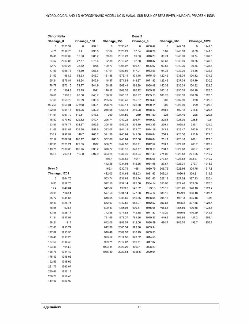
HYDROLOGICAL AND 1 D HYDRODYNAMIC MODELLING IN MANALI SUB-BASIN OF BEAS RIVER, HIMACHAL PRADESH, INDIA
Appendices 67
Chhor Nalla Beas 5 Chanage_0 Chanage_100 Chanage_150 Chanage_0 Chanage_560 Chanage_1020
0 2023.32 0 1999.1 0 2030.47 0 2030.47 0 1949.39 0 1942.5
4.71 2019.76 9.41 1995.5 37.64 2026.29 37.64 2026.29 0.89 1948.39 0.89 1941.5
15.45 2009.39 16.33 1985.2 59.83 2016.23 59.83 2016.23 30.74 1946.39 30.74 1939.5
24.57 2003.86 27.57 1978.6 92.88 2010.37 92.88 2010.37 60.65 1943.49 60.65 1936.6
32.72 1999.23 38.72 1965 109.77 1996.97 109.77 1996.97 90.56 1940.39 90.56 1933.5
47.89 1995.73 43.89 1955.5 117.01 1983.56 117.01 1983.56 94.38 1939.39 94.38 1932.5
51.63 1981.9 51.63 1943.7 131.48 1975.19 131.48 1975.19 120.42 1938.39 120.42 1931.5
65.24 1976.84 63.24 1942.6 148.37 1971.83 148.37 1971.83 125.49 1937.39 125.49 1930.5
78.77 1973.15 71.77 1941.9 168.88 1968.48 168.88 1968.48 150.32 1936.39 150.32 1929.5
81.15 1964.2 79.15 1941 176.12 1969.32 176.12 1969.32 180.18 1935.39 180.18 1928.5
86.68 1960.9 83.68 1940.7 186.97 1965.13 186.97 1965.13 188.76 1933.39 188.76 1926.5
97.69 1959.79 92.69 1939.6 205.07 1963.46 205.07 1963.46 200 1932.39 200 1925.5
99.258 1959.34 97.258 1939.1 226.78 1960.11 226.78 1960.11 209 1927.39 209 1920.5
102.05 1964.16 103.05 1939.9 246.08 1958.43 246.08 1958.43 218.6 1927.2 218.6 1920.4
111.51 1967.79 112.51 1943.6 269 1957.59 269 1957.59 226 1927.49 226 1920.6
118.82 1973.62 122.82 1949.4 296.74 1949.22 296.74 1949.22 228.5 1928.39 228.5 1921
123.87 1976.77 131.87 1952.5 305.19 1943.35 305.19 1943.35 239.1 1928.2 239.1 1921.2
131.68 1981.82 138.68 1957.6 322.07 1944.19 322.07 1944.19 243.9 1928.47 243.9 1921.2
133.7 1992.92 146.7 1968.7 341.38 1940.84 341.38 1940.84 256.9 1928.36 256.9 1921.3
137.12 2007.54 166.12 1980.3 357.06 1940.84 357.06 1940.84 261.1 1928.16 261.1 1921.3
142.35 2021.21 172.35 1987 366.71 1942.52 366.71 1942.52 263.7 1927.78 263.7 1920.9
149.75 2030.38 186.75 1996.2 378.77 1939.16 378.77 1939.16 268.7 1927.63 268.7 1920.8
156.8 2032.1 197.8 1997.9 393.24 1937.49 393.24 1937.49 271.05 1926.53 271.05 1919.7
404.1 1936.65 404.1 1936.65 273.67 1926.53 273.67 1919.7
412.55 1934.98 412.55 1934.98 273.7 1925.31 273.7 1918.5
Beas 5 466.1 1930.79 466.1 1930.79 306.75 1923.66 305.75 1917.8
Chanage_1251 482.03 1931.63 482.03 1931.63 309.21 1926.4 309.21 1919.6
0 1964.75 503.74 1931.63 503.74 1931.63 327.13 1927.24 327.13 1920.4
6.85 1957.75 522.56 1934.14 522.56 1934.14 353.06 1927.48 353.06 1920.6
17.4 1949.04 542.82 1933.3 542.82 1933.3 378.16 1928.28 378.16 1921.4
29.35 1948.1 577.56 1934.14 577.56 1934.14 386.16 1929.9 386.16 1923.1
35.72 1944.65 616.65 1936.65 616.65 1936.65 395.16 1931.8 395.16 1925
39.43 1926.74 662.97 1942.52 662.97 1942.52 397.66 1935.2 397.66 1928.4
48.56 1925.8 690.47 1955.08 690.47 1955.08 406.68 1956.66 406.68 1933.8
53.56 1925.17 742.58 1971.83 742.58 1971.83 419.29 1960.6 410.29 1942.8
71.34 1917.94 781.66 1979.37 781.66 1979.37 449.2 1969.95 427.2 1953.1
88.21 1917 812.06 1988.59 812.06 1988.59 484.7 1983.55 492.7 1955.7
102.43 1915.74 872.86 2005.34 872.86 2005.34
117.67 1913.55 910.49 2009.53 910.49 2009.53
128.48 1913.23 923.52 2014.56 923.52 2014.56
137.56 1914.49 959.71 2017.07 959.71 2017.07
153.45 1914.8 1003.14 2026.29 1003.1 2026.29
168.76 1914.49 1055.49 2029.64 1055.5 2029.64
175.43 1916.06
192.53 1916.69
221.73 1943.07
230.46 1952.18
238.78 1959.45
147.92 1967.32

HYDROLOGICAL AND 1 D HYDRODYNAMIC MODELLING IN MANALI SUB-BASIN OF BEAS RIVER, HIMACHAL PRADESH, INDIA
Appendices 68
Manalsu Nalla Beas 6 Chanage_0 Chanage_300 Chanage_460 Chanage_0 Chanage_105 Chanage_540
0 1943 0 1929 0 1964.75 0 1964.75 0 1960 0 1915
4 1940.2 0.25 1925.13 6.85 1957.75 6.85 1957.75 63.7 1953 2.87 1905.39
5 1937.8 3.75 1924.08 17.4 1949.04 17.4 1949.04 134.62 1944.3 13.1 1900.7
9 1938.2 7.31 1921.98 29.35 1948.1 29.35 1948.1 155.85 1943.4 22.2 1899.1
14 1937.5 9.39 1921.87 35.72 1944.65 35.72 1944.65 178.53 1939.9 23.6 1897.9
22.5 1932 11.69 1921.2 39.43 1926.74 39.43 1926.74 213.27 1922 43.1 1899.2
31.2 1930 13.2 1920.8 48.56 1925.8 48.56 1925.8 217.61 1921.1 47.79 1905.39
38.2 1928.5 14.2 1921.28 53.56 1925.17 53.56 1925.17 228.71 1920.4 61.64 1910.1
46.9 1930 18.1 1921.74 71.34 1917.94 71.34 1917.94 252.83 1913.2 88.83 1912.5
70.4 1941 19.83 1922.47 88.21 1917 88.21 1917 256.69 1912.3 97.27 1922.98
72.6 1941.1 21.29 1922.78 102.4 1915.74 102.43 1915.74 264.41 1911 122.44 1931.78
23.5 1923.33 117.7 1913.55 117.67 1913.55 274.55 1908.8 123.9 1943
25.97 1924.18 128.5 1913.23 128.48 1913.23 279.37 1908.5
26.74 1924.84 137.6 1914.49 137.56 1914.49 290.47 1909.7
28.19 1925.55 153.5 1914.8 153.45 1914.8 297.23 1910.1 Beas 6
168.8 1914.49 168.76 1914.49 308.81 1909.7 Chanage_975
175.4 1916.06 175.43 1916.06 322.32 1911.3 0 1996
192.5 1916.69 192.53 1916.69 328.59 1911.9 69.96 1948.36
221.7 1943.07 221.73 1943.07 341.62 1938.3 109.05 1940.3
230.5 1952.18 230.46 1952.18 371.05 1947.4 165.98 1905.12
238.8 1959.45 238.78 1959.45 196.55 1890.12
147.9 1967.32 147.92 1967.32 200 1892.4
201.9 1888.76
205.15 1888.26
209.55 1886.86
212 1885.41
212.5 1884.83
215.04 1884.11
226.4 1883.64
235.72 1882.7
240.84 1882.6
242.84 1882.9
244.84 1883.28
247.94 1885
250.88 1884.2
252.88 1888.7
254.88 1892.4
262.43 1892.5
267.64 1892.8
294.67 1898
327.4 1902.5
357.32 1913.5
387.2 1923.5
389.07 1933.5

HYDROLOGICAL AND 1 D HYDRODYNAMIC MODELLING IN MANALI SUB-BASIN OF BEAS RIVER, HIMACHAL PRADESH, INDIA
Appendices 69
Table 9-3: Temperature and Rainfall data from May to October at Bahang_SASE Gauge Station
Date Temperature (DEG-C)
Rainfall (mm) Date
Temperature (DEG-C)
Rainfall (mm) Date
Temperature (DEG-C)
Rainfall (mm)
1-May-95 19.4 0 1-May-99 20.75 0 1-May-00 18.75 0 2-May-95 18.6 0 2-May-99 21 5.6 2-May-00 19 0 3-May-95 18.4 20 3-May-99 16 3.4 3-May-00 21.25 0 4-May-95 19.2 0 4-May-99 18.5 0 4-May-00 20.75 19.5 5-May-95 18.3 0 5-May-99 17.5 0 5-May-00 19 16.6 6-May-95 18.4 0 6-May-99 17.5 0 6-May-00 17 10.3 7-May-95 19.3 0 7-May-99 20.45 0 7-May-00 14 6 8-May-95 19.7 0 8-May-99 20.9 0 8-May-00 17.5 0 9-May-95 18.5 0 9-May-99 20.25 9 9-May-00 18.75 0
10-May-95 19.2 0 10-May-99 11.75 0 10-May-00 20.25 0 11-May-95 19.2 0.6 11-May-99 18 0.6 11-May-00 20.75 0 12-May-95 19.4 0 12-May-99 16.25 0 12-May-00 21.5 18.2 13-May-95 19.75 0 13-May-99 16.4 7.4 13-May-00 19.75 17.7 14-May-95 20.15 0 14-May-99 14.5 1.4 14-May-00 19.25 0 15-May-95 22.55 0 15-May-99 15 0 15-May-00 20.5 0 16-May-95 23.25 0 16-May-99 16.15 0 16-May-00 18.25 23 17-May-95 22 0 17-May-99 17.25 0 17-May-00 19 0 18-May-95 19.25 0 18-May-99 18.5 1.6 18-May-00 19.25 13.8 19-May-95 15.7 16.5 19-May-99 17.75 2.4 19-May-00 19.75 1 20-May-95 15.2 5.4 20-May-99 17.75 0 20-May-00 20 0 21-May-95 15.55 1.6 21-May-99 19.25 0 21-May-00 19 0 22-May-95 14.7 6.6 22-May-99 18.9 0 22-May-00 20.1 0 23-May-95 15.45 0 23-May-99 19 3.4 23-May-00 20.4 22.6 24-May-95 15.7 0 24-May-99 19.5 63 24-May-00 19.4 15.3 25-May-95 15.7 0 25-May-99 15.25 38.8 25-May-00 20.75 0 26-May-95 18.9 0 26-May-99 11.75 3.2 26-May-00 19.25 17.4 27-May-95 18.8 0 27-May-99 18.1 0 27-May-00 20.4 0 28-May-95 19.4 0 28-May-99 19.25 0 28-May-00 18.35 10 29-May-95 19.45 0 29-May-99 20 6.2 29-May-00 18.75 0 30-May-95 19.5 0 30-May-99 18.75 1.4 30-May-00 19.25 8.2 31-May-95 20.4 0.2 31-May-99 18.65 2.4 31-May-00 19.35 13.4
1-Jun-95 22.35 0 1-Jun-99 17.1 6.6 1-Jun-00 17.25 0 2-Jun-95 21.85 0 2-Jun-99 15.75 0 2-Jun-00 19.25 0 3-Jun-95 21.95 0 3-Jun-99 15 0 3-Jun-00 20.25 0 4-Jun-95 23 0 4-Jun-99 14.25 5.6 4-Jun-00 19.5 0 5-Jun-95 22.5 0 5-Jun-99 13.75 3 5-Jun-00 15.25 0 6-Jun-95 22.5 0 6-Jun-99 12 0 6-Jun-00 20.25 0 7-Jun-95 22.85 0 7-Jun-99 14.9 0 7-Jun-00 19.5 0.4 8-Jun-95 22.75 0 8-Jun-99 18.75 0 8-Jun-00 17 33 9-Jun-95 22.9 0 9-Jun-99 20.75 0 9-Jun-00 16 19
10-Jun-95 24.4 0 10-Jun-99 20.5 16.3 10-Jun-00 17 4.2 11-Jun-95 23.6 0 11-Jun-99 21 0 11-Jun-00 16.25 0 12-Jun-95 22.2 0 12-Jun-99 20.25 0 12-Jun-00 17.75 0 13-Jun-95 21.25 0 13-Jun-99 20.1 0 13-Jun-00 17.75 0 14-Jun-95 21.75 0 14-Jun-99 19.25 0 14-Jun-00 21.25 0 15-Jun-95 23.05 0 15-Jun-99 19 0 15-Jun-00 20 0 16-Jun-95 24.65 0 16-Jun-99 20 0 16-Jun-00 22.5 13 17-Jun-95 23.2 0 17-Jun-99 21.5 0 17-Jun-00 22 0 18-Jun-95 20.55 0 18-Jun-99 23 12.4 18-Jun-00 21.5 14 19-Jun-95 19.8 6 19-Jun-99 20.7 0 19-Jun-00 22 0
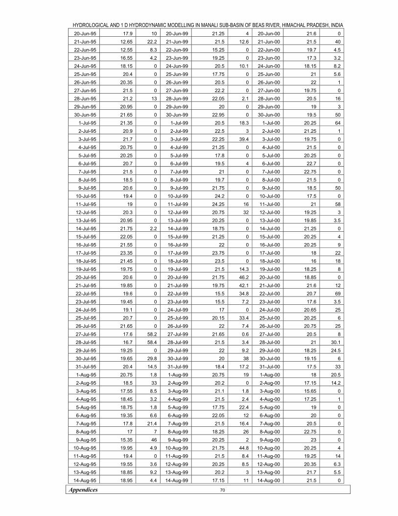
HYDROLOGICAL AND 1 D HYDRODYNAMIC MODELLING IN MANALI SUB-BASIN OF BEAS RIVER, HIMACHAL PRADESH, INDIA
Appendices 70
20-Jun-95 17.9 10 20-Jun-99 21.25 4 20-Jun-00 21.6 0 21-Jun-95 12.65 22.2 21-Jun-99 21.5 12.6 21-Jun-00 21.5 40 22-Jun-95 12.55 8.3 22-Jun-99 15.25 0 22-Jun-00 19.7 4.5 23-Jun-95 16.55 4.2 23-Jun-99 19.25 0 23-Jun-00 17.3 3.2 24-Jun-95 18.15 0 24-Jun-99 20.5 10.1 24-Jun-00 18.15 8.2 25-Jun-95 20.4 0 25-Jun-99 17.75 0 25-Jun-00 21 5.6 26-Jun-95 20.35 0 26-Jun-99 20.5 0 26-Jun-00 22 1 27-Jun-95 21.5 0 27-Jun-99 22.2 0 27-Jun-00 19.75 0 28-Jun-95 21.2 13 28-Jun-99 22.05 2.1 28-Jun-00 20.5 16 29-Jun-95 20.95 0 29-Jun-99 20 0 29-Jun-00 19 3 30-Jun-95 21.65 0 30-Jun-99 22.95 0 30-Jun-00 19.5 50
1-Jul-95 21.35 0 1-Jul-99 20.5 18.3 1-Jul-00 20.25 64 2-Jul-95 20.9 0 2-Jul-99 22.5 3 2-Jul-00 21.25 1 3-Jul-95 21.7 0 3-Jul-99 22.25 39.4 3-Jul-00 19.75 0 4-Jul-95 20.75 0 4-Jul-99 21.25 0 4-Jul-00 21.5 0 5-Jul-95 20.25 0 5-Jul-99 17.8 0 5-Jul-00 20.25 0 6-Jul-95 20.7 0 6-Jul-99 19.5 4 6-Jul-00 22.7 0 7-Jul-95 21.5 0 7-Jul-99 21 0 7-Jul-00 22.75 0 8-Jul-95 18.5 0 8-Jul-99 19.7 0 8-Jul-00 21.5 0 9-Jul-95 20.6 0 9-Jul-99 21.75 0 9-Jul-00 18.5 50
10-Jul-95 19.4 0 10-Jul-99 24.2 0 10-Jul-00 17.5 0 11-Jul-95 19 0 11-Jul-99 24.25 16 11-Jul-00 21 58 12-Jul-95 20.3 0 12-Jul-99 20.75 32 12-Jul-00 19.25 3 13-Jul-95 20.95 0 13-Jul-99 20.25 0 13-Jul-00 19.85 3.5 14-Jul-95 21.75 2.2 14-Jul-99 18.75 0 14-Jul-00 21.25 0 15-Jul-95 22.05 0 15-Jul-99 21.25 0 15-Jul-00 20.25 4 16-Jul-95 21.55 0 16-Jul-99 22 0 16-Jul-00 20.25 9 17-Jul-95 23.35 0 17-Jul-99 23.75 0 17-Jul-00 18 22 18-Jul-95 21.45 0 18-Jul-99 23.5 0 18-Jul-00 16 18 19-Jul-95 19.75 0 19-Jul-99 21.5 14.3 19-Jul-00 18.25 8 20-Jul-95 20.6 0 20-Jul-99 21.75 46.2 20-Jul-00 18.85 0 21-Jul-95 19.85 0 21-Jul-99 19.75 42.1 21-Jul-00 21.6 12 22-Jul-95 19.6 0 22-Jul-99 15.5 34.8 22-Jul-00 20.7 69 23-Jul-95 19.45 0 23-Jul-99 15.5 7.2 23-Jul-00 17.6 3.5 24-Jul-95 19.1 0 24-Jul-99 17 0 24-Jul-00 20.65 25 25-Jul-95 20.7 0 25-Jul-99 20.15 33.4 25-Jul-00 20.25 6 26-Jul-95 21.65 0 26-Jul-99 22 7.4 26-Jul-00 20.75 25 27-Jul-95 17.6 58.2 27-Jul-99 21.65 0.6 27-Jul-00 20.5 8 28-Jul-95 16.7 58.4 28-Jul-99 21.5 3.4 28-Jul-00 21 30.1 29-Jul-95 19.25 0 29-Jul-99 22 9.2 29-Jul-00 18.25 24.5 30-Jul-95 19.65 29.8 30-Jul-99 20 38 30-Jul-00 19.15 6 31-Jul-95 20.4 14.5 31-Jul-99 18.4 17.2 31-Jul-00 17.5 33 1-Aug-95 20.75 1.8 1-Aug-99 20.75 19 1-Aug-00 18 20.5 2-Aug-95 18.5 33 2-Aug-99 20.2 0 2-Aug-00 17.15 14.2 3-Aug-95 17.55 8.5 3-Aug-99 21.1 1.8 3-Aug-00 15.65 0 4-Aug-95 18.45 3.2 4-Aug-99 21.5 2.4 4-Aug-00 17.25 1 5-Aug-95 18.75 1.8 5-Aug-99 17.75 22.4 5-Aug-00 19 0 6-Aug-95 19.35 6.6 6-Aug-99 22.05 12 6-Aug-00 20 0 7-Aug-95 17.8 21.4 7-Aug-99 21.5 16.4 7-Aug-00 20.5 0 8-Aug-95 17 7 8-Aug-99 18.25 26 8-Aug-00 22.75 0 9-Aug-95 15.35 46 9-Aug-99 20.25 2 9-Aug-00 23 0
10-Aug-95 19.95 4.9 10-Aug-99 21.75 44.8 10-Aug-00 20.25 4 11-Aug-95 19.4 0 11-Aug-99 21.5 8.4 11-Aug-00 19.25 14 12-Aug-95 19.55 3.6 12-Aug-99 20.25 8.5 12-Aug-00 20.35 6.3 13-Aug-95 18.85 9.2 13-Aug-99 20.2 3 13-Aug-00 21.7 5.5 14-Aug-95 18.95 4.4 14-Aug-99 17.15 11 14-Aug-00 21.5 0

HYDROLOGICAL AND 1 D HYDRODYNAMIC MODELLING IN MANALI SUB-BASIN OF BEAS RIVER, HIMACHAL PRADESH, INDIA
Appendices 71
15-Aug-95 19.4 0 15-Aug-99 14.75 0 15-Aug-00 21.9 3 16-Aug-95 20.55 0 16-Aug-99 19.1 0 16-Aug-00 19.75 0 17-Aug-95 20.15 53.8 17-Aug-99 19.35 0 17-Aug-00 21.25 0 18-Aug-95 19.95 7.6 18-Aug-99 19.6 0 18-Aug-00 21.2 0 19-Aug-95 19.3 11.2 19-Aug-99 21.9 0 19-Aug-00 21.5 6 20-Aug-95 19.7 35.2 20-Aug-99 19.7 6 20-Aug-00 20.4 0 21-Aug-95 18.05 5 21-Aug-99 19.9 5.2 21-Aug-00 21.75 2 22-Aug-95 17.9 30.4 22-Aug-99 19.25 0 22-Aug-00 21.25 0 23-Aug-95 19.5 0.3 23-Aug-99 21.25 0 23-Aug-00 20.25 10.5 24-Aug-95 19.5 3.2 24-Aug-99 21.25 0 24-Aug-00 20.4 3 25-Aug-95 19.45 1 25-Aug-99 21.5 0 25-Aug-00 20.9 0 26-Aug-95 20 24.6 26-Aug-99 21.4 11 26-Aug-00 20.65 0 27-Aug-95 21.5 1.2 27-Aug-99 19.55 3.8 27-Aug-00 22.65 8.5 28-Aug-95 18.55 39.2 28-Aug-99 19.25 0 28-Aug-00 20.25 4 29-Aug-95 17.85 0.6 29-Aug-99 18.55 0 29-Aug-00 20.5 3 30-Aug-95 17.9 13.8 30-Aug-99 19 0 30-Aug-00 21 22 31-Aug-95 17.7 41.3 31-Aug-99 18.7 0 31-Aug-00 19.85 20
1-Sep-95 19.1 13.2 1-Sep-99 19.3 0 1-Sep-00 19.6 39 2-Sep-95 18.25 39 2-Sep-99 20.4 3 2-Sep-00 16.25 28.4 3-Sep-95 17.6 61.8 3-Sep-99 20.25 0.8 3-Sep-00 20.5 0 4-Sep-95 13.25 103.2 4-Sep-99 18.25 0 4-Sep-00 21.95 0 5-Sep-95 14 54 5-Sep-99 19.3 21.6 5-Sep-00 22.5 38.2 6-Sep-95 14.5 6 6-Sep-99 20.1 10 6-Sep-00 21.5 12 7-Sep-95 15.5 0 7-Sep-99 20.5 2 7-Sep-00 18.25 17.5 8-Sep-95 15.75 1.3 8-Sep-99 16.5 4.2 8-Sep-00 17.25 8 9-Sep-95 15.6 2.6 9-Sep-99 19.65 2 9-Sep-00 15.65 3
10-Sep-95 15.8 0 10-Sep-99 18 0 10-Sep-00 15.65 4 11-Sep-95 16.1 0 11-Sep-99 19.6 0 11-Sep-00 16.75 3.4 12-Sep-95 16.6 2 12-Sep-99 20.1 0 12-Sep-00 17.25 0 13-Sep-95 16.4 0 13-Sep-99 19.4 0 13-Sep-00 18.35 0 14-Sep-95 16.75 0 14-Sep-99 19.25 0 14-Sep-00 18.85 0 15-Sep-95 16.45 0 15-Sep-99 20.5 0 15-Sep-00 18.7 0 16-Sep-95 15.1 0 16-Sep-99 21.25 8.4 16-Sep-00 19.1 0 17-Sep-95 16.9 0 17-Sep-99 19.8 0 17-Sep-00 21 0 18-Sep-95 17.35 0 18-Sep-99 21.6 0 18-Sep-00 21 10.6 19-Sep-95 17.1 0 19-Sep-99 21.75 3.6 19-Sep-00 19.35 6.1 20-Sep-95 16.8 0 20-Sep-99 21.5 17 20-Sep-00 17.5 18 21-Sep-95 17.35 0 21-Sep-99 17.75 0 21-Sep-00 15.5 25.3 22-Sep-95 17.15 0 22-Sep-99 20 0 22-Sep-00 17 6.3 23-Sep-95 17.05 0 23-Sep-99 22.1 2 23-Sep-00 15.25 0 24-Sep-95 18.9 0.6 24-Sep-99 20.1 4.8 24-Sep-00 15 0 25-Sep-95 16.5 0 25-Sep-99 16.25 7 25-Sep-00 15.25 5.3 26-Sep-95 16.8 0 26-Sep-99 18.75 0 26-Sep-00 15.5 18.5 27-Sep-95 16.75 0 27-Sep-99 18.5 0 27-Sep-00 11.25 0 28-Sep-95 15.15 16.2 28-Sep-99 18.5 0 28-Sep-00 14.75 0 29-Sep-95 15.9 1.4 29-Sep-99 19.25 0 29-Sep-00 15 0 30-Sep-95 15.05 0 30-Sep-99 19.8 12 30-Sep-00 15.5 0
1-Oct-95 15.95 0 1-Oct-99 19.45 0 1-Oct-00 17 0 2-Oct-95 16.2 0 2-Oct-99 16.85 0 2-Oct-00 16.75 32 3-Oct-95 15 0 3-Oct-99 17.25 0 3-Oct-00 16.75 27.4 4-Oct-95 14.2 0 4-Oct-99 17.25 0 4-Oct-00 17.5 15.6 5-Oct-95 14.85 0 5-Oct-99 17.1 0 5-Oct-00 18 4.8 6-Oct-95 16.75 0 6-Oct-99 17.75 0 6-Oct-00 18.5 0.7 7-Oct-95 16.1 0 7-Oct-99 17.3 3.6 7-Oct-00 18.75 0 8-Oct-95 16.55 0 8-Oct-99 16.9 1 8-Oct-00 18 0 9-Oct-95 17.2 0 9-Oct-99 12.75 0 9-Oct-00 15.75 0
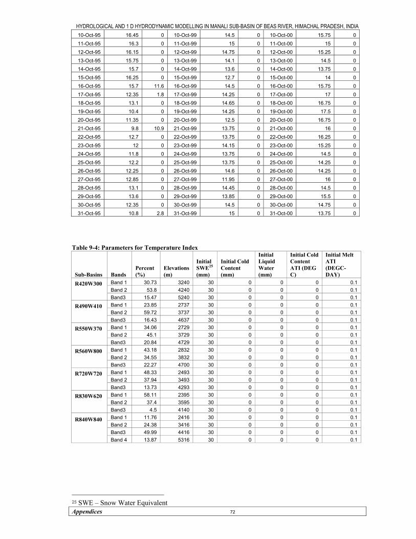
HYDROLOGICAL AND 1 D HYDRODYNAMIC MODELLING IN MANALI SUB-BASIN OF BEAS RIVER, HIMACHAL PRADESH, INDIA
Appendices 72
10-Oct-95 16.45 0 10-Oct-99 14.5 0 10-Oct-00 15.75 0 11-Oct-95 16.3 0 11-Oct-99 15 0 11-Oct-00 15 0 12-Oct-95 16.15 0 12-Oct-99 14.75 0 12-Oct-00 15.25 0 13-Oct-95 15.75 0 13-Oct-99 14.1 0 13-Oct-00 14.5 0 14-Oct-95 15.7 0 14-Oct-99 13.6 0 14-Oct-00 13.75 0 15-Oct-95 16.25 0 15-Oct-99 12.7 0 15-Oct-00 14 0 16-Oct-95 15.7 11.6 16-Oct-99 14.5 0 16-Oct-00 15.75 0 17-Oct-95 12.35 1.8 17-Oct-99 14.25 0 17-Oct-00 17 0 18-Oct-95 13.1 0 18-Oct-99 14.65 0 18-Oct-00 16.75 0 19-Oct-95 10.4 0 19-Oct-99 14.25 0 19-Oct-00 17.5 0 20-Oct-95 11.35 0 20-Oct-99 12.5 0 20-Oct-00 16.75 0 21-Oct-95 9.8 10.9 21-Oct-99 13.75 0 21-Oct-00 16 0 22-Oct-95 12.7 0 22-Oct-99 13.75 0 22-Oct-00 16.25 0 23-Oct-95 12 0 23-Oct-99 14.15 0 23-Oct-00 15.25 0 24-Oct-95 11.8 0 24-Oct-99 13.75 0 24-Oct-00 14.5 0 25-Oct-95 12.2 0 25-Oct-99 13.75 0 25-Oct-00 14.25 0 26-Oct-95 12.25 0 26-Oct-99 14.6 0 26-Oct-00 14.25 0 27-Oct-95 12.85 0 27-Oct-99 11.95 0 27-Oct-00 16 0 28-Oct-95 13.1 0 28-Oct-99 14.45 0 28-Oct-00 14.5 0 29-Oct-95 13.6 0 29-Oct-99 13.85 0 29-Oct-00 15.5 0 30-Oct-95 12.35 0 30-Oct-99 14.5 0 30-Oct-00 14.75 0 31-Oct-95 10.8 2.8 31-Oct-99 15 0 31-Oct-00 13.75 0
Table 9-4: Parameters for Temperature Index
Sub-Basins Bands Percent (%)
Elevations (m)
Initial SWE25 (mm)
Initial Cold Content (mm)
Initial Liquid Water (mm)
Initial Cold Content ATI (DEG C)
Initial Melt ATI (DEGC-DAY)
Band 1 30.73 3240 30 0 0 0 0.1 Band 2 53.8 4240 30 0 0 0 0.1
R420W300 Band3 15.47 5240 30 0 0 0 0.1
Band 1 23.85 2737 30 0 0 0 0.1 Band 2 59.72 3737 30 0 0 0 0.1
R490W410 Band3 16.43 4637 30 0 0 0 0.1
Band 1 34.06 2729 30 0 0 0 0.1 Band 2 45.1 3729 30 0 0 0 0.1
R550W370 Band3 20.84 4729 30 0 0 0 0.1
Band 1 43.18 2832 30 0 0 0 0.1 Band 2 34.55 3832 30 0 0 0 0.1
R560W800 Band3 22.27 4700 30 0 0 0 0.1
Band 1 48.33 2493 30 0 0 0 0.1 Band 2 37.94 3493 30 0 0 0 0.1
R720W720 Band3 13.73 4293 30 0 0 0 0.1
Band 1 58.11 2395 30 0 0 0 0.1 Band 2 37.4 3595 30 0 0 0 0.1
R830W620 Band3 4.5 4140 30 0 0 0 0.1
Band 1 11.76 2416 30 0 0 0 0.1 Band 2 24.38 3416 30 0 0 0 0.1 Band3 49.99 4416 30 0 0 0 0.1
R840W840 Band 4 13.87 5316 30 0 0 0 0.1
25 SWE – Snow Water Equivalent

HYDROLOGICAL AND 1 D HYDRODYNAMIC MODELLING IN MANALI SUB-BASIN OF BEAS RIVER, HIMACHAL PRADESH, INDIA
Appendices 73
Figure 9-1 Feature Space of Landsat ETM+ Image

HYDROLOGICAL AND 1 D HYDRODYNAMIC MODELLING IN MANALI SUB-BASIN OF BEAS RIVER, HIMACHAL PRADESH, INDIA
Appendices 74
Appendix-3: Simulated Results of HEC-HMS and MIKE 11 Table 9-5: Changes in Discharge at Manali Outlet, 2000 in HEC-HMS
Time
Discharge (m3/S) for L/G 2
Discharge (m3/S) for L/G 0.5
Discharge (m3/S) for Im2
Discharge (m3/S) for Im 0.5
Discharge (m3/S) -Validated
Observed Discharge (m3/S)
MAY I 496.56 535.46 522.27 494.46 503.63 675
MAY II 637.3 691.15 658.73 642.44 647.91 887
MAY III 795.01 863.16 811.62 808 809.25 967
JUN I 782.9 848.25 796.5 795.37 795.74 735
JUN II 701.32 757.92 711.98 711.61 711.71 737
JUN III 999.96 1086.45 1018.52 1017.6 1017.85 1027
JUL I 1147.44 1243.34 1167.68 1167.09 1167.26 1023
JUL II 1167.35 1264 1187.48 1187.1 1187.23 1100
JUL III 1601.91 1740.16 1632.08 1631.7 1631.81 1894
AUG I 1146.46 1225.48 1161.85 1161.79 1161.8 1115
AUG II 1132.63 1207.74 1146.83 1146.78 1146.8 878
AUG III 1339.93 1432.21 1358.14 1358.07 1358.08 1327
SEP I 1069.24 1161.09 1090.3 1090.17 1090.22 1098
SEP II 602.88 649.32 612.21 612.19 612.21 801
SEP III 693.78 749.57 705.64 705.58 705.6 767
OCT I 696.66 753.23 709.2 709.14 709.17 642
OCT II 414.2 442.4 419.64 419.7 419.64 578
OCT III 454.77 486.08 461.32 461.16 460.7 534
Figure 9-2: Graphical Representation of Result for 1995 in HEC-HMS
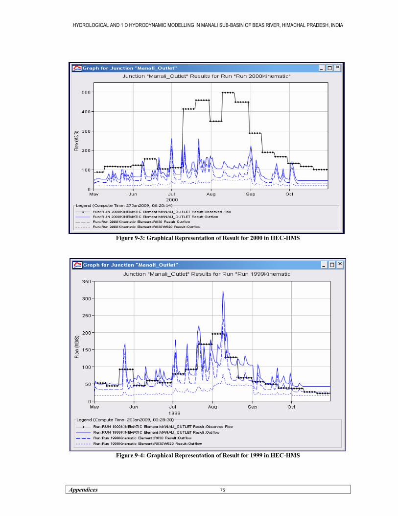
HYDROLOGICAL AND 1 D HYDRODYNAMIC MODELLING IN MANALI SUB-BASIN OF BEAS RIVER, HIMACHAL PRADESH, INDIA
Appendices 75
Figure 9-3: Graphical Representation of Result for 2000 in HEC-HMS
Figure 9-4: Graphical Representation of Result for 1999 in HEC-HMS

HYDROLOGICAL AND 1 D HYDRODYNAMIC MODELLING IN MANALI SUB-BASIN OF BEAS RIVER, HIMACHAL PRADESH, INDIA
Appendices 76
Rainfall and Observed Discharge Relation, 1999
y = 8.1352x + 302.55R2 = 0.8806
0
500
1000
1500
2000
2500
0 50 100 150 200 250
Rainfall in mm
Disc
harg
e in
m3/
S
1999 Observed Discharge
Linear (1999 ObservedDischarge)
Figure 9-5: Relation between 10 Daily Rainfalls and Simulated Discharge in 1999 in HEC-HMS
Rainfall and Simulated Discharge Relation, 1999y = 5.5338x + 519.58
R2 = 0.7279
0200400600800
10001200140016001800
0 50 100 150 200 250
Rainfall in mm
Dis
char
ge in
m3/
S
1999 Simulated Dischrge
Linear (1999 SimulatedDischrge )
Figure 9-6: 10 Daily Total Rainfalls and Observed Discharge Relation for the Year 1999 in HEC-HMS
Figure 9-7: Time Series Water Level (1st) and Longitudinal Profile (2nd) of Main Beas River, 2000
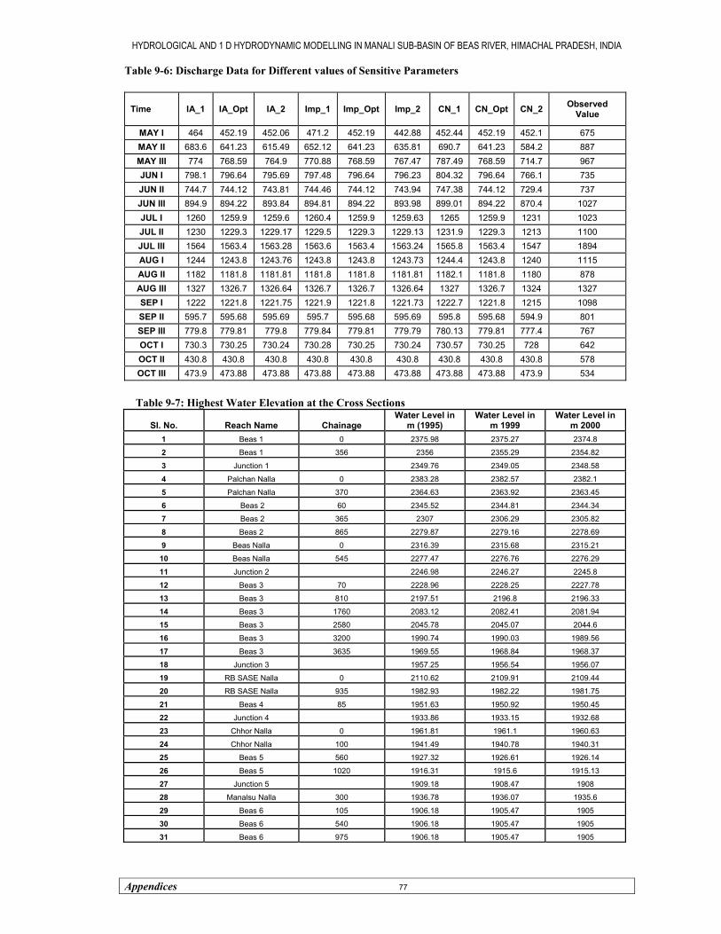
HYDROLOGICAL AND 1 D HYDRODYNAMIC MODELLING IN MANALI SUB-BASIN OF BEAS RIVER, HIMACHAL PRADESH, INDIA
Appendices 77
Table 9-6: Discharge Data for Different values of Sensitive Parameters
Time IA_1 IA_Opt IA_2 Imp_1 Imp_Opt Imp_2 CN_1 CN_Opt CN_2 Observed Value
MAY I 464 452.19 452.06 471.2 452.19 442.88 452.44 452.19 452.1 675 MAY II 683.6 641.23 615.49 652.12 641.23 635.81 690.7 641.23 584.2 887 MAY III 774 768.59 764.9 770.88 768.59 767.47 787.49 768.59 714.7 967 JUN I 798.1 796.64 795.69 797.48 796.64 796.23 804.32 796.64 766.1 735 JUN II 744.7 744.12 743.81 744.46 744.12 743.94 747.38 744.12 729.4 737 JUN III 894.9 894.22 893.84 894.81 894.22 893.98 899.01 894.22 870.4 1027 JUL I 1260 1259.9 1259.6 1260.4 1259.9 1259.63 1265 1259.9 1231 1023 JUL II 1230 1229.3 1229.17 1229.5 1229.3 1229.13 1231.9 1229.3 1213 1100 JUL III 1564 1563.4 1563.28 1563.6 1563.4 1563.24 1565.8 1563.4 1547 1894 AUG I 1244 1243.8 1243.76 1243.8 1243.8 1243.73 1244.4 1243.8 1240 1115 AUG II 1182 1181.8 1181.81 1181.8 1181.8 1181.81 1182.1 1181.8 1180 878 AUG III 1327 1326.7 1326.64 1326.7 1326.7 1326.64 1327 1326.7 1324 1327 SEP I 1222 1221.8 1221.75 1221.9 1221.8 1221.73 1222.7 1221.8 1215 1098 SEP II 595.7 595.68 595.69 595.7 595.68 595.69 595.8 595.68 594.9 801 SEP III 779.8 779.81 779.8 779.84 779.81 779.79 780.13 779.81 777.4 767 OCT I 730.3 730.25 730.24 730.28 730.25 730.24 730.57 730.25 728 642 OCT II 430.8 430.8 430.8 430.8 430.8 430.8 430.8 430.8 430.8 578 OCT III 473.9 473.88 473.88 473.88 473.88 473.88 473.88 473.88 473.9 534
Table 9-7: Highest Water Elevation at the Cross Sections
Sl. No. Reach Name Chainage Water Level in
m (1995) Water Level in
m 1999 Water Level in
m 2000 1 Beas 1 0 2375.98 2375.27 2374.8
2 Beas 1 356 2356 2355.29 2354.82
3 Junction 1 2349.76 2349.05 2348.58
4 Palchan Nalla 0 2383.28 2382.57 2382.1
5 Palchan Nalla 370 2364.63 2363.92 2363.45
6 Beas 2 60 2345.52 2344.81 2344.34
7 Beas 2 365 2307 2306.29 2305.82
8 Beas 2 865 2279.87 2279.16 2278.69
9 Beas Nalla 0 2316.39 2315.68 2315.21
10 Beas Nalla 545 2277.47 2276.76 2276.29
11 Junction 2 2246.98 2246.27 2245.8
12 Beas 3 70 2228.96 2228.25 2227.78
13 Beas 3 810 2197.51 2196.8 2196.33
14 Beas 3 1760 2083.12 2082.41 2081.94
15 Beas 3 2580 2045.78 2045.07 2044.6
16 Beas 3 3200 1990.74 1990.03 1989.56
17 Beas 3 3635 1969.55 1968.84 1968.37
18 Junction 3 1957.25 1956.54 1956.07
19 RB SASE Nalla 0 2110.62 2109.91 2109.44
20 RB SASE Nalla 935 1982.93 1982.22 1981.75
21 Beas 4 85 1951.63 1950.92 1950.45
22 Junction 4 1933.86 1933.15 1932.68
23 Chhor Nalla 0 1961.81 1961.1 1960.63
24 Chhor Nalla 100 1941.49 1940.78 1940.31
25 Beas 5 560 1927.32 1926.61 1926.14
26 Beas 5 1020 1916.31 1915.6 1915.13
27 Junction 5 1909.18 1908.47 1908
28 Manalsu Nalla 300 1936.78 1936.07 1935.6
29 Beas 6 105 1906.18 1905.47 1905
30 Beas 6 540 1906.18 1905.47 1905
31 Beas 6 975 1906.18 1905.47 1905
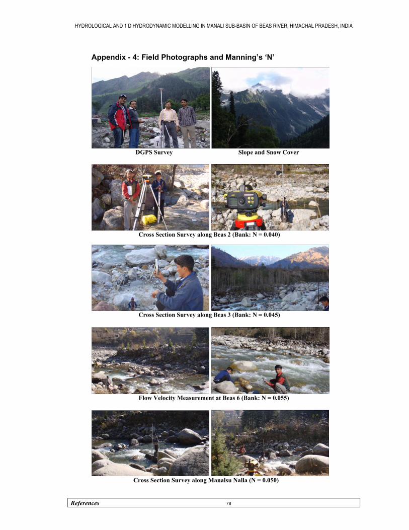
HYDROLOGICAL AND 1 D HYDRODYNAMIC MODELLING IN MANALI SUB-BASIN OF BEAS RIVER, HIMACHAL PRADESH, INDIA
References 78
Appendix - 4: Field Photographs and Manning’s ‘N’
DGPS Survey Slope and Snow Cover
Cross Section Survey along Beas 2 (Bank: N = 0.040)
Cross Section Survey along Beas 3 (Bank: N = 0.045)
Flow Velocity Measurement at Beas 6 (Bank: N = 0.055)
Cross Section Survey along Manalsu Nalla (N = 0.050)
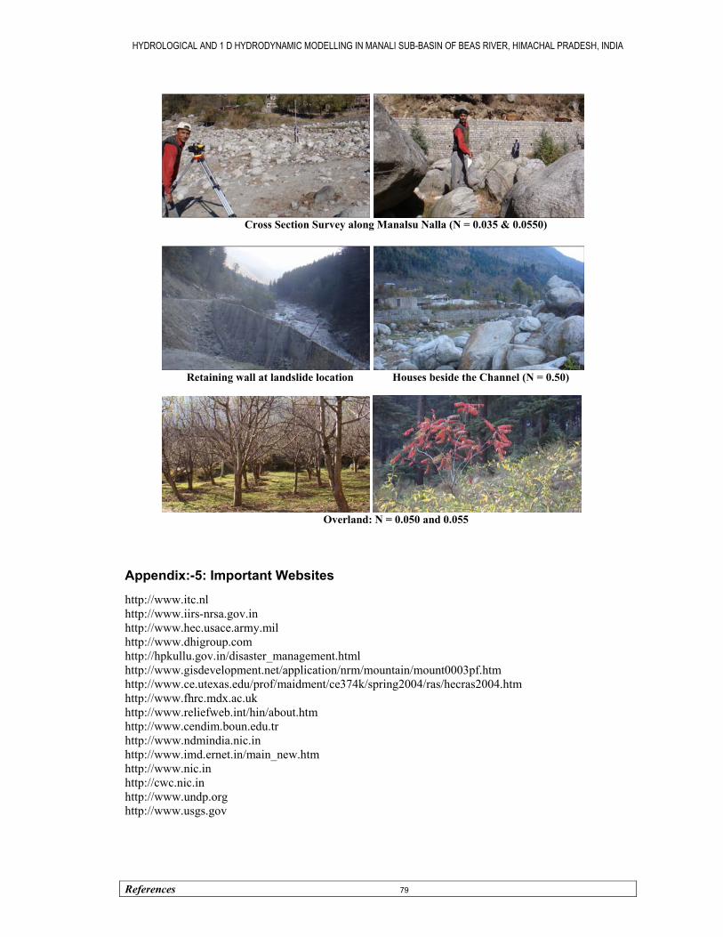
HYDROLOGICAL AND 1 D HYDRODYNAMIC MODELLING IN MANALI SUB-BASIN OF BEAS RIVER, HIMACHAL PRADESH, INDIA
References 79
Cross Section Survey along Manalsu Nalla (N = 0.035 & 0.0550)
Retaining wall at landslide location Houses beside the Channel (N = 0.50)
Overland: N = 0.050 and 0.055
Appendix:-5: Important Websites
http://www.itc.nl http://www.iirs-nrsa.gov.in http://www.hec.usace.army.mil http://www.dhigroup.com http://hpkullu.gov.in/disaster_management.html http://www.gisdevelopment.net/application/nrm/mountain/mount0003pf.htm http://www.ce.utexas.edu/prof/maidment/ce374k/spring2004/ras/hecras2004.htm http://www.fhrc.mdx.ac.uk http://www.reliefweb.int/hin/about.htm http://www.cendim.boun.edu.tr http://www.ndmindia.nic.in http://www.imd.ernet.in/main_new.htm http://www.nic.in http://cwc.nic.in http://www.undp.org http://www.usgs.gov