Hydrodynamic Modeling of Towed Buoyant Submarine ...

Hydrodynamic Modeling of Towed Buoyant Submarine

Antenna's in Multidirectional Seas

by

Sam R. Geiger

B.S., Louisiana Tech University, 1993

Submitted to the Department of Ocean Engineering, MITand to the Department of Applied Ocean Physics and Engineering, WHOI

in partial fulfillment of the requirements for the degree of

Master of Science in Oceanographic Engineering

at the

MASSACHUSETTS INSTITUTE OF TECHNOLOGY

and the

WOODS HOLE OCEANOGRAPHIC INSTITUTION

September 2000

© 2000 Sam R. GeigerAll rights reserved.

The author herebyelectronic copies of

Signature of Author..

grants to MIT and WHOI permission to reproduce paper andthis thesis in whole or in part and to distribute them publicly.

.................../ ...... 4...... .. . r ......................Joint Program in Oceanographic Engineering

Massachusetts Institute of Technologyand Woods Hole Oceanographic Institution

August 4, 2000

C ertified by ... .. . ...... .. ...... . .. . . . . . . . . . . . .. . .. . . . .Jerome H. Milgram

Professor, Ocean EngineeringThesis Supervisor

Accepted by... .. .. ..... .. - ... ............ 1 .. . . . .. ....

Professor Micha CSS. TriantafyllouChair, Joint Committee for Oceanographic Engineering

Massachusetts Institute of Technologyand Woods Hole Oceanographic Institution

MASSA1i CHST SISTITUTEOF TECHNOLOGY

MAR 2 7 2001

LIBRARIES

B ARKER

Hydrodynamic Modeling of Towed Buoyant Submarine Antenna's in

Multidirectional Seas

by

Sam R. Geiger

Submitted to the Department of Ocean Engineering, MITand to the Department of Applied Ocean Physics and Engineering, WHOI

on August 4, 2000 in partial fulfillment of the requirements for the degree ofMaster of Science in Oceanographic Engineering

Abstract

A finite difference computer model is developed to simulate the exposure statistics of a radiofrequency buoyant antenna as it is towed in a three-dimensional random seaway. The modelallows the user to prescribe antenna properties (length, diameter, density, etc.), sea conditions(significant wave height, development of sea), tow angle, and tow speed. The model thensimulates the antenna-sea interaction for the desired duration to collect statistics relating toantenna performance. The model provides design engineers with a tool to predict antennaperformance trends, and to conduct design tradeoff studies. The floating antenna envisionedis for use by a submarine operating at modest speed and depth.

Thesis Supervisor: Jerome H. MilgramTitle: Professor, Ocean Engineering

2

Contents

1 Introduction

1.1 Motivation

1.2

1.3

Background . . . . . . . . . . . . . . . . . . . . .

Antenna Model . . . . . . . . . . . . . . . . . . .

2 Wave Field Model Development

2.1 Linear, Random, Deep Water Wave Theory . . .

2.2 Energy Density Spectra Contained in the Model

2.2.1 Bretschneider Two Parameter Spectrum

2.2.2 Ochi Six Parameter Spectrum . . . . . . .

2.2.3 Square Wave Spectrum . . . . . . . . . .

2.2.4 Single Sine Wave Spectrum . . . . . . . .

2.3 Unidirectional Modeling Methods . . . . . . . . .

2.3.1 Sine Wave Superposition (SWS) Method.

2.3.2 Fast Fourier Transform (FFT) Method . .

2.4 Multidirectional Modeling Methods . . . . . . . .

2.4.1 Complete Wave Field (CWF) Method . .

2.4.2 Partial Wave Field (PWF) Method . . . .

2.5 Verification of Model Seas . . . . . . . . . . . . .

2.5.1 Significant Wave Height . . . . . . . . . .

2.5.2 Encounter Frequency . . . . . . . . . . . .

2.5.3 Spatial Spectral Analysis . . . . . . . . .

. . . . . . . 10

.. - - - 11

12

. . . . . . . . . . . . . . . . . . 12

. . . . . . . . . . . . . . . . . . 16

. . . . . . . . . . . . . . . . . . 18

. . . . . . . . . . . . . . . . . . 20

. . . . . . . . . . . . . . . . . . 22

. . . . . . . . . . . . . . . . . . 22

. . . . . . . . . . . . . . . . . . 23

. . . . . . . . . . . . . . . . . . 24

. . . . . . . . . . . . . . . . . . 25

. . . . . . . . . . . . . . . . . . 28

. . . . . . . . . . . . . . . . . . 29

. . . . . . . . . . . . . . . . . . 34

. . . . . . . . . . . . . . . . . . 43

. . . . . . . . . . . . . . . . . . 43

. . . . . . . . . . . . . . . . . . 45

. . . . . . . . . . . . . . . . . . 46

3

9

S . 9

2.5.4 Temporal Spectral Analysis . . . . . . . . . . . . . . . . . . . . . . . . .4

3 Antenna Model Development

3.1 Coordinate System Description .......

3.2 Governing Vertical Equation of Motion . .

3.3 Antenna Modeling Methods . . . . . . . .

3.3.1 Discretization . . . . . . . . . . . .

3.3.2 Integration Method . . . . . . . .

3.3.3 Boundary Conditions . . . . . . .

3.3.4 Initial Conditions . . . . . . . . . .

4 Modeling Results

4.1 Exposure Statistics . . . . . . . . . . . . .

4.1.1 Definition of Exposure . . . . . . .

4.1.2 Statistics Calculated by the Model

4.2 Results . . . . . . . . . . . . . . . . . . . .

4.2.1 Series 1: Statistics vs. Number of

4.2.2 Series 2: Statistics vs. Tow Angle

4.2.3 Series 3: Statistics vs. Sea Severit

4.2.4 Series 4: Statistics vs. Tow Speed

4.2.5 Series 5: Statistics vs. Antenna L

4.2.6 Series 6: Statistics vs. Antenna D

4.2.7 Series 7: Statistics vs. Antenna D

51

. . . . . . . . . . . . . . 51

. . . . . . . . . . . . . . 53

. . . . . . . . . . . . . . 55

. . . . . . . . . . . . . . 55

. . . . . . . . . . . . . . 57

. . . . . . . . . . . . . . 58

. . . . . . . . . . . . . . 59

60

. . . . . . . . . . . . . . 60

. . . . . . . . . . . . . . 60

. . . . . . . . . . . . . . 61

Propagation Directions

..................

y. . . . . . . . . . . . .

mg..............ength . . . . . . . . . . .

iameter . . . . . . . . . .

ensity . . . . . . . . . . .

. . . . . . 63

. . . . . . 63

. . . . . . 65

. . . . . . 67

. . . . . . 69

. . . . . . 71

. . . . . . 73

. . . . . . 75

5 Future Efforts

A User's Guide to Proteus

A .1 Introduction . . . . . . . . . . . . . . . . . . . . . . . . . . . . . . . . . . . . . . .

A.1.1 Contents of the User's Guide . . . . . . . . . . . . . . . . . . . . . . . . .

A.1.2 Analysis Procedure . . . . . . . . . . . . . . . . . . . . . . . . . . . . . . .

A.2 Proteus Input File . . . . . . . . . . . . . . . . . . . . . . . . . . . . . . . . . . .

A.2.1 Description of Features and Limitations . . . . . . . . . . . . . . . . . . .

4

77

78

78

78

78

81

81

49

A.2.2 Sample Input File . . . . . . . . . . . . . . . . . . . . . . . . . . . . . . . 91

A .3 O utput Files . . . . . . . . . . . . . . . . . . . . . . . . . . . . . . . . . . . . . . 91

A.3.1 Snapshot Output File (run_ id//'_mat') . . . . . . . . . . . . . . . . . . 91

A.3.2 Simulation Parameters and Results File (run_ id//'_info.txt') . . . . . . 92

A.3.3 Exposure Data Matrix File (run_ id//'_edm') . . . . . . . . . . . . . . . 95

A.3.4 Temporal Wave Data File (run_ id//' mat2') . . . . . . . . . . . . . . . . 95

A.3.5 Spatial Wave Data File (run id//'_mat3') . . . . . . . . . . . . . . . . . 96

B Sea State Correlation Data 98

5

List of Figures

2-1 Typical Wave Energy Density Spectrum . . . . . . . . . . . . . . . . . . . . . . . 14

2-2 Determination of Component Amplitudes ai (w) . . . . . . . . . . . . . . . . . . . 15

2-3 Bretschneider Spectrum for Varying Sea Severity . . . . . . . . . . . . . . . . . . 18

2-4 Bretschneider Spectrum for Varying Degrees of Development . . . . . . . . . . . 19

2-5 Ochi Six Parameter Single Most Probable Spectrum . . . . . . . . . . . . . . . . 21

2-6 Square Wave Spectrum . . . . . . . . . . . . . . . . . . . . . . . . . . . . . . . . . 22

2-7 Single Sine Wave Spectrum . . . . . . . . . . . . . . . . . . . . . . . . . . . . . . 23

2-8 Complete Wave Field 3-D Energy Spectrum (quadrants 1 and 4 shown) . . . . . 31

2-9 Wave Field Generated by CWF Method . . . . . . . . . . . . . . . . . . . . . . . 34

2-10 PWF Unidirectional Wave Summation . . . . . . . . . . . . . . . . . . . . . . . . 35

2-11 Partial Wave Field 3-D Energy Spectrum - No Directional Scaling (quadrants 1

and 4 shown) . . . . . . . . . . . . . . . . . . . . . . . . . . . . . . . . . . . . . . 36

2-12 Cosine Square Directional Spreading Function . . . . . . . . . . . . . . . . . . . . 38

2-13 Cosine Square Directional Spreading Function for the Five Directions Example

P roblem . . . . . . . . . . . . . . . . . . . . . . . . . . . . . . . . . . . . . . . . . 38

2-14 Partial Wave Field 3-D Energy Spectrum - With Directional Scaling (quadrants

1 and 4 shown) . . . . . . . . . . . . . . . . . . . . . . . . . . . . . . . . . . . . . 39

2-15 Geometry of the Wave Summation . . . . . . . . . . . . . . . . . . . . . . . . . . 41

2-16 Encounter Frequency for Varying Tow Speeds . . . . . . . . . . . . . . . . . . . . 45

2-17 Spectral Analysis of Spatial Wave Data - One Propagation Direction . . . . . . . 46

2-18 Spectral Analysis of Spatial Wave Data - Three Propagation Directions . . . . . 47

2-19 Spectral Analysis of Spatial Wave Data - Five Propagation Directions . . . . . . 48

6

2-20 Spatial Frequency Stretching

2-21 Spectral Analysis of Temporal Wave Data . . . . . . . . . . . . . . . . . . . . . .

3-1 Coordinate System: X-Z Plane . . . . . . . . . . . . . . . . . . . . . . . . . . . .

3-2 Coordinate System: X-Y Plane . . . . . . . . . . . . . . . . . . . . . . . . . . . .

3-3 Antenna and Sea Surface Elevation Variables . . . . . . . . . . . . . . . . . . . .

3-4 Antenna Element Description . . . . . . . . . . . . . . . . . . . . . . . . . . . . .

3-5 Antenna and Antenna Element Description . . . . . . . . . . . . . . . . . . . . .

4-1

4-2

4-3

4-4

4-5

4-6

4-7

A-i

A-2

A-3

Average Exposure vs. Number of Propagation Directions

Average Exposure vs. Tow Angle . . . . . . . . . . . . . .

Average Exposure vs. Sea Severity . . . . . . . . . . . . .

Average Exposure vs. Tow Speed . . . . . . . . . . . . . .

Average Exposure vs. Antenna Length . . . . . . . . . . .

Average Exposure vs. Antenna Diameter . . . . . . . . .

Average Exposure vs. Antenna Density . . . . . . . . . .

Sample Threshold Antenna Exposure of 0.04 . . . . . . .

Sample Output of Snapshot Output File . . . . . . . . . .

Sample Output of Temporal Wave Data Analysis . . . . .

A-4 Sample Output of Spatial Wave Data Analysis

7

. . . . . . . . . . . . . 64

. . . . . . . . . . . . . 66

. . . . . . . . . . . . . 68

. . . . . . . . . . . . . 70

. . . . . . . . . . . . . 72

. . . . . . . . . . . . . 74

. . . . . . . . . . . . . 76

. . . . . . . . . . . . . 89

. . . . . . . . . . . . . 92

. . . . . . . . . . . . . 96

97

50

52

52

54

55

56

. . . . . . . . . . . . 4 9

List of Tables

2.1 Linear Theory Deep Water Wave Relations . . . . . . . . . . . . . . . . . . . . . 13

2.2 Ochi Six Parameter Spectrum: Most Probable Values . . . . . . . . . . . . . . . 21

2.3 Comparison of Fourier Transform Domain Relationships . . . . . . . . . . . . . . 25

2.4 Comparison of Frequency Resolution for the SWS and FFT Methods . . . . . . . 28

2.5 Simulated Significant Wave Heights for a Specified Sea Severity of 3.0 m . . . . . 44

4.1 Series 1 Input Parameters . . . . . . . . . . . . . . . . . . . . . . . . . . . . . . . 63







B.1 Sea State Correlation Data . . . . . . . . . . . . . . . . . . . . . . . . . . . . . . 99

8

Chapter 1

Introduction

1.1 Motivation

As the United States Navy launches the last of the highly capable Seawolf class submarines and

begins construction on the even more capable Virginia class submarines, it continues to find itself

operationally limited by the technological barriers present with high data rate communications.

The capability for high speed data transfer has escalated at an astonishing rate over the last

few years; however, the submarine force faces unique challenges in fully utilizing high data

rate systems which operate at higher frequencies. High frequency (UHF, SHF, or EHF band)

radio signals are unable to penetrate below the surface of the water; so, while the submarine

is submerged, radio communications systems are limited to low data rate receive-only modes

transmitted at very low frequencies (ELF, or VLF band). The current mode of operation calls

for the submarine to routinely come to periscope depth to raise a radio mast above the surface of

the water, send and receive the necessary message traffic, then submerge to continue its mission.

This required visit to periscope depth not only causes the submarine to suspend execution

of its mission, but also reduces the overall stealth of the mission. Submarine operations

are typically driven by the need for stealth, and stealth is best preserved by remaining fully

submerged. Clearly, the communications goal of the submarine force is to be able to utilize

the high frequency and high data rate communication circuits while retaining the stealth of

operation at speed and depth.

9

1.2 Background

This goal of high data rate communication at speed and depth is the motivation of a U.S. Navy

Advanced Technology Demonstration (ATD). Initially funded jointly by the Defense Advanced

Research Projects Agency (DARPA) and the Office of Naval Research (ONR) in FY 96-97 as

a feasibility study, the Buoyant Cable Array Antenna (BCAA) research became a DARPA and

ONR Demonstration in FY 98-99. The BCAA prototype satisfactorily demonstrated receive-

only capability with a field test in the Summer of 1999. The program was promoted to the level

of Navy ATD in FY 00 and renamed the Multi-element Buoyant Cable Antenna (MBCA). The

MBCA is a 3 year joint program which is a combined Navy ATD-funded and DARPA-funded

effort. This ATD, one of only 6 ATD's funded by the Navy for fiscal year 2000, reflects the

high priority the Navy places on submarine connectivity. The goals of the MBCA program

include:

" demonstrate 24 kbps 2-way communication at UHF over the Fleet Satellite (FLTSAT)

communications system while the submarine is at a speed of 6 knots and at a depth of

300 feet

" demonstrate 1.5 Mbps data rates over UHF Line-of-Site

" demonstrate L-band voice communications.

The participants in the program include the Naval Undersea Warfare Center, Johns Hopkins

University Applied Physics Laboratory, Sippican Inc., and MIT's Lincoln Laboratory. Lincoln

Laboratory is a federally funded laboratory administered by the Massachusetts Institute of

Technology. Lincoln Laboratory, whose specialties include radar and electrical engineering,

was chosen to overcome the technological challenge of designing a floating linear array radio

frequency communication antenna module and the associated inboard electronics. However, to

gain insight into the behavior of the antenna module in a random seaway, Lincoln Laboratory

added Professor Jerome Milgram of the MIT Ocean Engineering department to the antenna

development effort. Professor Milgram joined a working group that was established to estimate

statistics on

9 the average fraction of antenna elements exposed over an extended period of time

10

" the temporal variation of the exposure statistics, including duration of reception dropout

times

" the spatial distribution of those exposed elements.

This thesis work was undertaken to support the statistics working group by improving upon

the first hydrodynamic model which was developed by Professor Milgram and Gary Ulrich.

[9][10] The improved model retains all of the capabilities of the original model and improves

upon the original model by upgrading the wave field from a unidirectional wave field with the

choice of only two tow directions, 0 or 180 degrees, to a multidirectional wave field with the

choice of any tow direction from 0 to 180 degrees. This provides all angles due to port and

starboard symmetry.

1.3 Antenna Model

The method used to determine the antenna behavior and the exposure statistics was to develop

long term simulations from which exposure statistics could be obtained vice getting the exposure

statistics from the theory of a non-linear process. The model, named PROTEUS, performs

the simulation by constructing a wave field and then modeling the antenna in the wave field

and analyzing the resultant behavior. The development of the wave field model is described in

Chapter 2 and the development of the antenna model is described in Chapter 3. The results

of the improved model are presented in Chapter 4 and a detailed user's guide is included as

Appendix A.

11

Chapter 2

Wave Field Model Development

2.1 Linear, Random, Deep Water Wave Theory

To simplify the model and to reduce computation time, the simulated wave field was assumed to

be described by linear, random, deep-water wave theory. The linear theory aspect of the waves

implies that the velocity potential and fluid velocity are constant from the mean free-surface to

the free-surface level. The linear theory assumptions represent a first order approximation in

satisfying the free surface kinematic and dynamic boundary conditions. A complete derivation

and discussion of linear wave theory can be found in Faltinsen and Newman. [4][6] "Deep

water" is defined to exist when A < 2d, where A is the wavelength and d is the water depth.

The random aspect of the waves implies that

" the instantaneous wave elevation from the mean free-surface is gaussian distributed with

zero mean and variance

" the waves are an ergodic process, which means that the wave statistics obtained from a

single location are the same as the wave statistics obtained from an ensemble of locations

" the waves are a stationary process, which means that the wave statistics are invariant

with respect to time [7][8]

Because the last condition is so restrictive, we relax it to allow the statistics to vary slowly

with time, otherwise known as a weakly-stationary process. A summary of the deep water

linear theory wave relations is provided in Table 2.1.

12

Quantity Formula

Wave Number k =Circular Frequency w = 7r

2

Dispersion Relation k =g

Velocity Potential = 3ekz sin(kx' - wt)Surface Displacement h a cos(kx' - wt)Radian Frequency w = fgkPhase Velocity c = g/kGroup Velocity C = g/kHorizontal Fluid Velocity u = awekz cos(kx' - wt)Vertical Fluid Velocity w = awekz sin(kx' - wt)Wave Energy Density E = ipga2

Note: x' refers to a stationary x coordinate system.

Table 2.1: Linear Theory Deep Water Wave Relations

Assuming a lower wave frequency bound of 0.3 rad/sec, which is reasonable for the vast

majority of energy density spectra one would encounter, this translates into a minimum water

depth of 342 meters. This implies that for depths shallower than about 350 meters, the

deep water theory begins to break down, and a finite depth treatment of the waves must be

considered. A complete derivation and discussion of finite depth wave theory can be found in

Faltinsen and Newman. [4][6]

Upon inspection of the linear theory formulas in Table 2.1, the waves are found to be

sinusoidal. However, an observation of the sea surface shows that the waves display a quite

complicated and random structure. This observed behavior can be numerically approximated

by adding together a series of sinusoids with each discrete frequency component having the

appropriate amplitude and a random phase. As the number of discrete frequency components

increases, the numerical approximation approaches the continuous distribution of the actual

sea surface. This discrete method of describing a two dimensional random seaway is presented

in Equation 2.1

N

h(x', t) = a (w) cos(ki(w)x' - wit + #i) (2.1)

where

13

Bretschneider Energy Density Spectrum1.4

1.2-

e 0.8

E

3 0.6-(1)

0.4-

0.2-

0-0 0.5 1 1.5 2 2.5 3

Frequency (rad/sec)

Figure 2-1: Typical Wave Energy Density Spectrum

h(x', t) is the wave elevation, referenced to the mean free-surface

a2 (w) is the appropriate wave amplitude of each discrete frequency component

ki(w) is the wave number of each discrete frequency component

wi is the set of discrete circular frequencies contained in the modeled energy density spectrum

Oi is the random phase assigned to each discrete frequency component

and the ekz term has been dropped, since evaluation occurs at the sea surface (z = 0).

Using the equations found in Table 2.1, one can determine most of the terms on the right

hand side of Equation 2.1: ki is determined from the dispersion relation, and Oi is a random

number with a uniform distribution on 0 to 27r. The determination of the appropriate wave

amplitude, however, requires some discussion and a deeper understanding of wave theory.

To determine the wave amplitude corresponding to a given wave frequency, one begins by

defining the spectral energy density function, S(w), which represents the energy of the waves

having frequency w. A typical energy density spectrum is shown in Figure 2-1. The units of

S(w) are defined to be in m 2-sec, so that when S(w) is integrated with respect to w, the result

is the average energy of the random waves with respect to time.

14

Bretschneider Energy Density Spectrum

0.8 F

0.6 -

0.4

0.21

0.0 0.2 0.4 0.6 0.8 1 1.2Frequency (rad/sec)

1.4 1.6 1.8 2

Figure 2-2: Determination of Component Amplitudes ai (w)

The spectrum shown in Figure 2-1 is said to be a single-sided spectrum, which refers to

the fact that the frequencies are constrained to be positive. For a double-sided spectrum, both

the positive and the negative frequencies are allowed, and the spectrum is defined such that

S(w) = S(-w). In addition, the double-sided spectrum is half the magnitude of the single-sided

spectrum; since, for constant sea severity, the area under the spectral energy density curve must

be constant. The amplitudes, ai(w), of the discrete frequency components in Equation 2.1 are

obtained from Equation 2.2

1-a (O)2 = S(W)Aw2

(2.2)

where

ai(w) is the amplitude of the discrete band, Aw, of waves with center frequency w.

Equation 2.2 is simply a statement that the square of the wave amplitude is a measure of

the average energy of the waves, because both sides of the equation represent energy in units

of M 2 . The method of obtaining the amplitudes ai(w) is shown in Figure 2-2.

15

E

a.(co)=(2 S(0o) Aw)1/2

SA

Until now, S(w) has been presented in terms of wave energy present at a given wave fre-

quency. It can be shown from the Wiener-Khintchine theorem that S(w) is related to the wave

amplitude record at a fixed location in the ocean. [7] We define a wave record at a given

location as x'(t). Then the autocorrelation of x'(t) is given by

R(T) = lim jX'(t) X'(t + T) dt (2.3)T~oo 2T _T

and by the Wiener-Khintchine theorem, the spectral energy density function, S(w), and the

autocorrelation function, R(T), form a Fourier transform pair.

1 0S(w) = - R(T) e-iwrdT (2.4)

7r 1-0

R(T) = j S(w) 6iw'dw (2.5)

This method proves to be invaluable as it has the ability to convert observed wave records into

spectral energy density functions.

2.2 Energy Density Spectra Contained in the Model

Numerous energy density spectral forms have been proposed by researchers attempting to char-

acterize a particular sea wave environment. [4] [5] [7] [8] The spectral forms may characterize a

particular geographic wave environment or they may characterize a particular storm environ-

ment, but in all cases, they share a very similar form. The model incorporates the spectral

formulation as a subroutine; therefore, it is completely arbitrary from the model viewpoint how

the spectrum is defined. In order to provide some variability in the allowable spectral forms

and to allow for troubleshooting and debugging of the model, four wave spectral energy forms

were included in the model. Two of the spectral forms are actual derived models that are well

accepted in the ocean design field. Though the two spectral models may appear very different

at first glance, most spectral formulations share the basic form of Equation 2.6 [9]

S(w) A H e-BW(2.6):;w

16

where

A, B are constants to be determined

H, is the significant wave height, which is defined to be the average wave height of the

one third highest waves. Sea severity is most commonly given in terms of significant wave

height among researchers; however, significant data exists which gives sea severity in terms of

a value called sea state. Appendix B provides a correlation amongst significant wave height,

modal wave frequency, wind speed, and sea state. The two actual derived spectral formulations

chosen for the model are the Bretschneider two parameter spectrum and the Ochi six parameter

spectrum, given in Equations 2.7 and 2.8, respectively. [7]

S(w) = WH2,e1.25(wm/w)4 (2.7)4 w5

1 2 4A3-+IW4 .Aj H 2 (43+1) /j4S(W)= - E 4 ( 4 )m (2.8)

4 1-(Aj) W4A + I

The other two models are the square wave spectrum and the single sine wave spectrum,

given in Equations 2.9 and 2.10, respectively. These simple geometric form models were used

for troubleshooting and debugging of the model and to verify the results of the model.

0.0 for b < 0.01

S (b) = 5.0 for 0.01 < b < 1.01 (2.9)

0.0 for b > 1.01

S (b) = 56 (b - bs) (2.10)

where

17


(Development = 1.0 for all cases)

Hs3 mS

H =2 mS

H5 =1 m

2 2.5 3

Figure 2-3: Bretschneider Spectrum for Varying Sea Severity

kb = -

27

and b, is the spatial frequency of the sine wave.

(2.11)

2.2.1 Bretschneider Two Parameter Spectrum

The two parameters of the Bretschneider spectrum, Equation 2.7, are significant wave height,

H,, and modal frequency, win. Modal frequency is the frequency at which S(w) reaches its

maximum value, and significant wave height is as previously defined. For the special case of

a fully developed sea, a relationship exists between w, and H. A fully developed sea, also

referred to as a fully arisen sea, is one in which the wind imparts energy to the waves at a

rate equal to that at which viscous damping dissipates their energy and wave-wave interactions

transmit energy from one frequency to another. Designating this modal frequency as WMFA, we

18

1.4

1.2 -

0.8

E

9 0.6ZCo

0.4 -

0.2 -

00 0.5 1 1.5

Frequency (rad/sec)

Bretschneider Energy Density Spectrum(HS = 3.0 m for all cases)

1.6Development=0.75

1.4 -

1.2 -Deelopment=1.00

Q) Devlopment=1.25

E 0.8

' 0.6 -

0.4-

0.2

00 0.5 1 1.5 2 2.5 3

Frequency (rad/sec)

Figure 2-4: Bretschneider Spectrum for Varying Degrees of Development

have

WFA 04 '(2.12)

which establishes the energy equilibrium characteristic of a fully arisen sea. The two require-

ments for a fully developed sea are

" sufficient distance over which the wind is blowing over the water, or fetch

" sufficient length of time the wind has been blowing, or duration.

If the fetch or duration are insufficient, the modal frequency will be greater than that given

by Equation 2.12; if the winds are subsiding, the modal frequency will be less than that given

by Equation 2.12. This is best understood by considering the mechanism by which waves are

generated. The wind causes ripples, or capillary waves, on the sea surface, which is a short

wavelength, high frequency phenomenon. Thus as a storm is building, wave energy input occurs

at high frequency, and the energy gradually is transferred through wave-wave interactions to

lower frequencies. Likewise, as a storm is subsiding, the high frequency waves attenuate most

19

rapidly due to viscous effects, and the result is a skewing of the spectral energy toward lower

frequencies. By introducing a term we will call the development factor, Dev, we can quantify

the degree of sea arousal as given in Equation 2.13. [9]

wm = Dev WmFA (2.13)

Using this convention, values of Dev < 1.0 correspond to a decaying sea, and values of Dev > 1.0

correspond to a building sea. Figures 2-3 and 2-4 show representative plots of S(w) as significant

wave height and development, respectively, are varied. Note that in Figure 2-4, that while

changing the development shifts the location of peak spectral energy density, it keeps the area

under the curve,and thus the total energy, constant.

2.2.2 Ochi Six Parameter Spectrum

The Ochi six parameter spectrum is a generalization of the Bretschneider two parameter spec-

trum in two respects:

" two spectral peaks are present, each with their own modal frequency and significant wave

height, and their contributions add together

* a shape factor, A, can be applied to each spectral peak to skew the curve right or left,

independent of the significant wave height or modal frequency. [9]

In the form given in Equation 2.8, each parameter is an independent variable. However,

by analyzing over 800 wave spectra from the North Atlantic, Ochi obtained a relationship for

the six parameters in terms of the measured significant wave height, H. [7] The result of this

analysis is a family of spectra having a 95% confidence; however, the results given in Table

2.2 represent a single "most probable" spectrum [7]. The model implements this single most

probable form for obtaining the six parameters of the Ochi spectrum. A sample plot of the

Ochi most probable spectrum, showing its characteristic bimodal shape, is shown in Figure 2-5.

20

Parameter Value

Hs1 0.84H,

Hs 2 0.54HsUmI 0.70e-0.

04 6H,

Wm2 1.15e-0.039H,

A, 3.00A2 1.54e-- 0.06 2H

Table 2.2: Ochi Six Parameter Spectrum: Most Probable Values

Ochi Energy Density Spectrum(Single Most Probable Spectrum for Hs = 3.0 m)

1.8

1.6

1.4 [1.2 [

E0.8 -

0.6 [0.4 -

0.2

0 0.5 1.5 2 2.5Frequency (rad/sec)

Figure 2-5: Ochi Six Parameter Single Most Probable Spectrum

21

1

1

Square Wave Energy Density Spectrum7

6-

5-

4--

E

3-1-

2

0-0.2 0 0.2 0.4 0.6 0.8 1

Spatial Frequency (m- )

Figure 2-6: Square Wave Spectrum

2.2.3 Square Wave Spectrum

The square wave spectrum was added to the model to provide for verification of the resultant

multidirectional wave field spectral analysis. By providing a more easily recognizable input

spectrum, the goal was to generate a more easily recognizable output spectrum. A plot of the

square wave spectrum is shown in Figure 2-6.

2.2.4 Single Sine Wave Spectrum

The single sine wave spectrum was added to the model to provide for an efficient recognizable

input spectrum which could be used for troubleshooting the frequency related components of

the multidirectional wave field. By providing a more easily recognizable input spectrum, the

goal was to generate a more easily recognizable output spectrum. A plot of the single sine

wave spectrum is shown in Figure 2-7.

22

Single Sine Wawa Energy Density Spectrum7

6-

5-

4-

E

3-

2-

00 0.05 0.1 0.15 0.2 0.25 0.3 0.35 0.4

Spatial Frequency (m- 1 )

Figure 2-7: Single Sine Wave Spectrum

2.3 Unidirectional Modeling Methods

As mentioned earlier, the wave field in the previous model consisted of a unidirectional random

seaway with the choice of only two tow directions. The wave field in the current model makes

use of the unidirectional method to construct the multidirectional wave field, so it is necessary

to completely understand the unidirectional method developed by Ulrich before moving on

to the development of the multidirectional method. The discussion and derivation of the

unidirectional method that follows comes from Ulrich. [9]

The sea domain variables of interest for the unidirectional wave field are

" sea elevation, h

" fluid horizontal velocity, u

" fluid vertical velocity, w.

Two methods were employed in arriving at the sea domain properties of the unidirectional

wave field, each with certain advantages and disadvantages. The first method will be called

the Sine Wave Superposition (SWS) method, and the second method will be called the Fast

23

Fourier Transform (FFT) method. The source code for both of these computer programs can

be found in reference [10].

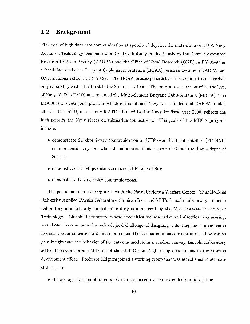
2.3.1 Sine Wave Superposition (SWS) Method

As previously mentioned in Equation 2.1, the sea elevation can be obtained by a superposition

of sine waves having a random phase and an amplitude prescribed by Equation 2.2. In like

manner, the fluid velocities can be calculated by the superposition method. The formulas for

h, u and w in an earth-fixed reference frame are provided in Equations. 2.14 - 2.16.

N

h(x', t) = 7 ai (w) cos(ki(w) x' - wit + #i) (2.14)

N

u(x', t) = a (w) w cos(ki(w) x' - wit + #i) (2.15)

N

w(x', t) = a (w) w sin(ki(w) x' - wit + #i) (2.16)i=21

By invoking a coordinate transformation and the dispersion relation from Table 2.1, one arrives

at the forms appropriate to the coordinate system moving with the antenna. These are presented

in Equations 2.17 - 2.19.

N

h(x, t) = I3ai(w)cos ki(w)x- (wi - U)t +#i] (2.17)

N= 1

u(x, t) = ai (w) w cos ki(w) x - (wi - ) (2.18)1 -k~)X

N w-U 1

w(x, t) = ai (w) w sin ki(w) x - (wi - )t+ #I (2.19)i=1 -~J

The spectral energy density function S(w) used in this formulation was a single sided spectrum.

The advantages of the SWS method are

" simplicity in coding fluid property subroutines

" good resolution for S(w) at lower frequencies, where most of the wave energy resides

24

Time-Frequency Space-Spatial Fre-Domain quency Domain

f = 1/T b 11Lw=2wf k=27rb

k = (2irf)2/g w = 2irgb

Table 2.3: Comparison of Fourier Transform Domain Relationships

9 frequency meshing (Aw) is unrelated to the spatial meshing (Ax), allowing both antenna

element length and wave energy frequency resolution to be arbitrarily chosen.

2.3.2 Fast Fourier Transform (FFT) Method

This method takes advantage of the fact that Equations 2.14 - 2.16 are a Fourier series, and

thus the functions h, U,and w are the inverse Fourier transform of some expression. Since the

calculations to determine the sea domain properties occur at a fixed point in time, the transform

variables are not w and t, rather they become b and x. Table 2.3 summarizes the analogous

relationships between the time-frequency domains and the space-spatial frequency domains.

Because the FFT algorithm used for the model assumed the presence of both positive and

negative frequency components, it was necessary to use a two sided spectrum for this method.

In order to retain the same amount of energy (i.e. area under the spectral energy density curve)

as the transition from one-sided to two-sided spectra is made, it is necessary that the formula

for the component amplitudes be adjusted from that given in Equation 2.2. In addition, it is

convenient to incorporate the random phase, #i, into a complex component amplitude, Ci. With

these changes in mind, the formulas providing the sea domain properties are given in Equations

2.20 - 2.24.

h(x) Re ci(bi) exp [i(27rbix + (27rbiU - 2ixgbi) t)] (2.20)

u(x) Re ci(bi) /2rgb, exp [i(2bix + (2wbiU - V2irgbi) t)] (2.21)

w NiU

w (x) =Re -ici (bi) V/2-7rgbi exp [I(27rbix + (27rbi U - V/2_7gbi) t) (2.22)

25

Re {ci(bi)} =

Im{ci(bi)} =

2 S(bi) Ab cos(#i)

2S(bi) Ab sin(oi)

Then the Fourier transform pairs become

H(b)

V/27rgbi H(b)

-i V27rg bi H(b)

N

Hib)

h(x)

Su(x)

w(x)

ci(b) exp [it (27rbiU - /27rgbi)]

H(b) * h(x) (2.29)

is defined to mean

H(b)

h(x)

N

= >3h(x) exp (-i27rbx)

N

27r3 H(b) exp (i27rbx)

(2.30)

(2.31)

By setting the complex component amplitudes, ci, to obey the relation

ci(bi) = ci(-bi) (2.32)

that is, the positive frequency components are the complex conjugates of the negative frequency

components, then the imaginary parts of Equations 2.20-2.22 are zero, and the Re{ } can be

26

(2.23)

(2.24)

where

(2.25)

(2.26)

(2.27)

and

(2.28)

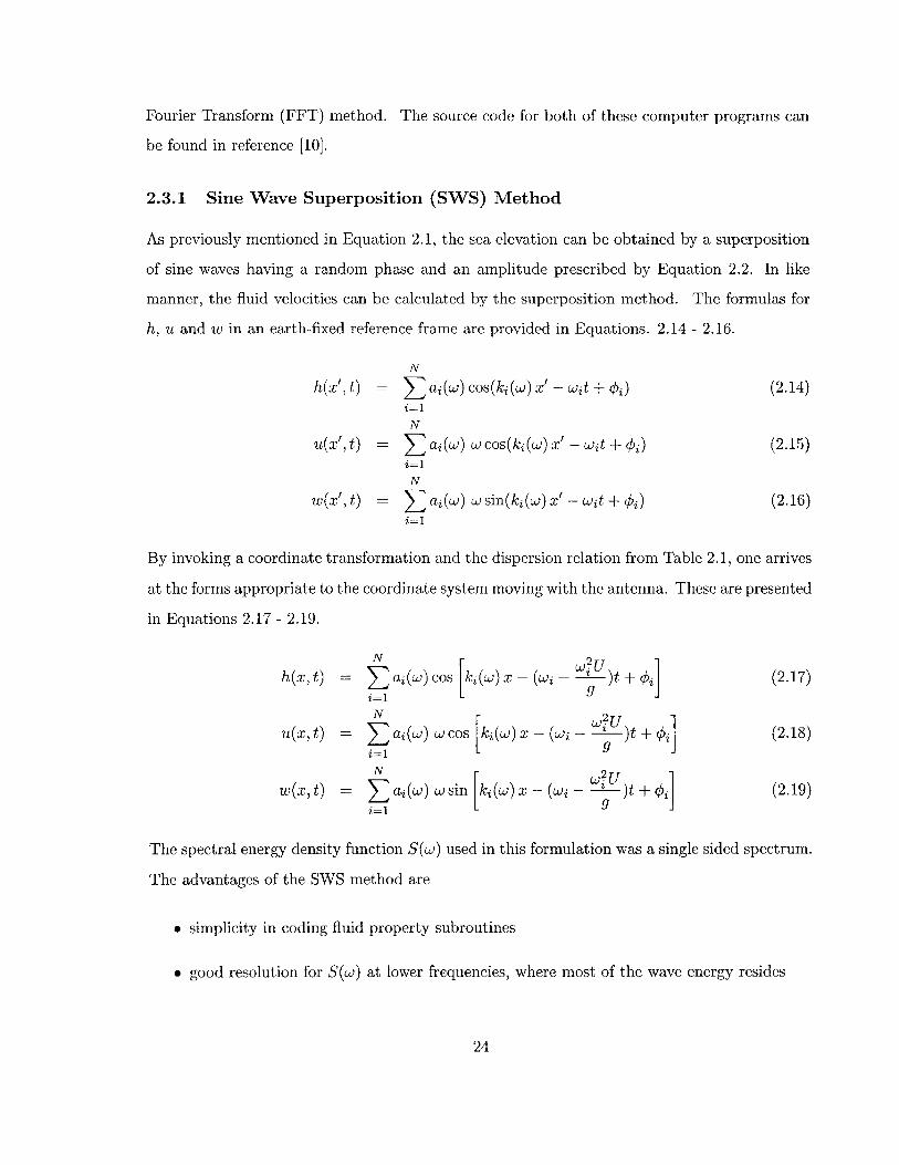
dropped from the equations. Finally, the wave field is constructed by performing an inverse

FFT on the one-dimensional complex arrays, represented by the left side of Equations 2.25 -

2.27, which contain the Fourier coefficients describing h, u, and w.

When converting between the spectral energy density function as a function of w to another

variable, such as b, the basic relations of Equations 2.33 and 2.34 are useful.

S(w) dw S(b) db (2.33)dw

S (b) = S(L) dw(2.34)d b

An important feature of the FFT method is the linkage of the spatial frequency domain

meshing (Ab), and the sea spatial meshing (Ax). The key to the FFT method is to make the

antenna spatial meshing, As, match the sea domain spatial meshing, Ax. This is accomplished

by using the relations given in Equations 2.35 - 2.38, and ensuring that the sea Ax equals the

desired antenna As.

Ab bmin (2.35)Lsea

NseaAb _Nsea 12 2Lsea 2Ax

Wmin = 27rgbmin (2.37)

Wmax = 2wrgbmax (2.38)

The primary advantage of the FFT method is computational speed. The FFT method

executes approximately 10 times faster than the SWS version. A further increase in execution

speed is accomplished by not computing the FFT every time step, At. Rather, the sea data

(h, u, w) is computed at nAt intervals, and linearly interpolated in between. The integer n is

determined by the computer model using the highest sea energy frequency component, Wmax.

This ensures that the linearly interpolated sea evolves in a smooth and continuous fashion.

Its disadvantage is that it has poorer low frequency resolution of the sea wave energy than its

SWS counterpart. This is demonstrated by a typical run case in Table 2.4 where the lowest 10

frequencies defined are listed for both methods. As one can readily calculate from integrating

Equation 2.7 with respect to w, for a sea severity of 2.0 m significant wave height, 67.7% of the

27

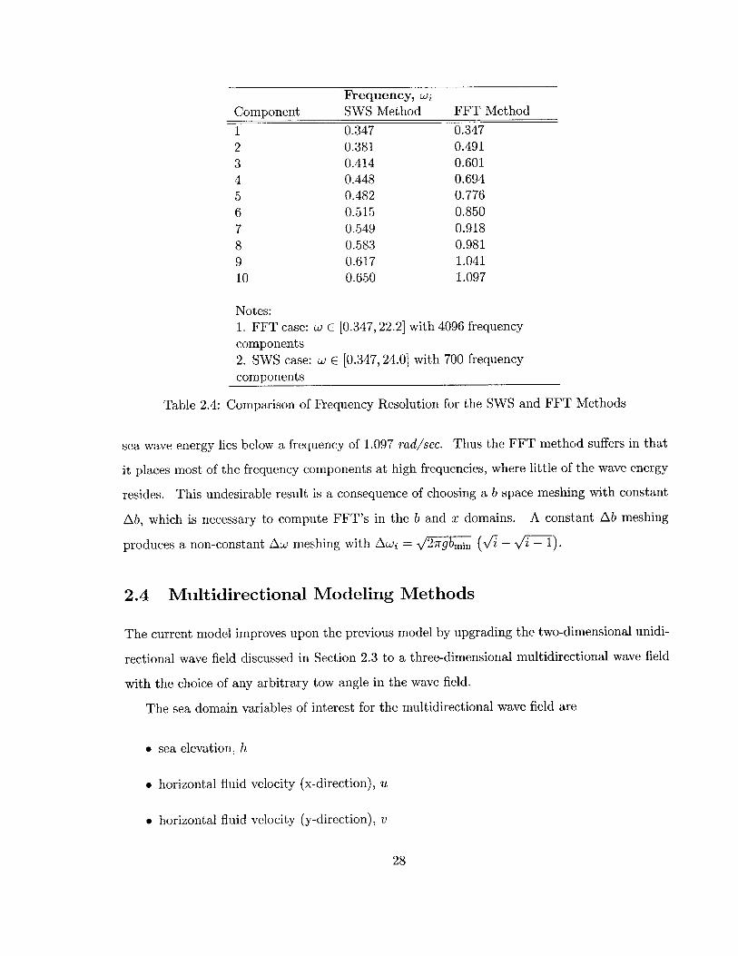
Frequency, wjSWS Method

0.3470.3810.4140.4480.4820.5150.5490.5830.6170.650

FFT Method

0.3470.4910.6010.6940.7760.8500.9180.9811.0411.097

Notes:1. FFT case: w E [0.347,22.2] with 4096 frequency

components

2. SWS case: w E [0.347,24.0] with 700 frequencycomponents

Table 2.4: Comparison of Frequency Resolution for the SWS and FFT Methods

sea wave energy lies below a frequency of 1.097 rad/sec. Thus the FFT method suffers in that

it places most of the frequency components at high frequencies, where little of the wave energy

resides. This undesirable result is a consequence of choosing a b space meshing with constant

Ab, which is necessary to compute FFT's in the b and x domains. A constant Ab meshing

produces a non-constant Aw meshing with Awi = v/2 7rgbmin (v' - i - 1).

2.4 Multidirectional Modeling Methods

The current model improves upon the previous model by upgrading the two-dimensional unidi-

rectional wave field discussed in Section 2.3 to a three-dimensional multidirectional wave field

with the choice of any arbitrary tow angle in the wave field.

The sea domain variables of interest for the multidirectional wave field are

" sea elevation, h

" horizontal fluid velocity (x-direction), u

* horizontal fluid velocity (y-direction), v

28

Component

12345678910

* vertical fluid velocity, w.

Two methods were considered in arriving at the sea domain properties of the multidirectional

wave field, each with certain advantages and disadvantages. The first method will be called

the Complete Wave Field (CWF) method, and the second will be called the Partial Wave Field

(PWF) method.

2.4.1 Complete Wave Field (CWF) Method

The Complete Wave Field (CWF) method involves the construction of a three-dimensional wave

field using a spectral energy model that is completely described in both the x and y directions

in the spatial frequency domain. This is accomplished in a manner similar to that discussed

in Section 2.3.2, except that the equations now will be a function of both x and y and will

separate the horizontal velocity into x and y components.

As previously mentioned in Equation 2.1, the sea elevation can be obtained by a superpo-

sition of sine waves having a random phase and an amplitude prescribed by Equation 2.2. In

like manner, the fluid velocities can be calculated by the superposition method. The formulas

for h, u, v, and w in an earth-fixed reference frame are provided in Equations 2.39 - 2.42.

N N

h(x', y', t) = 3 aj>(3 x, wyk) cos(kx, (ox ) x' + kyk (wy) y' - Wjkt + Ojk) (2.39)j=1 k=1

N N

u(',y', t) = EEajk(x,, WYk) Wjk cos (Ojk) (2.40)j=1 k=1

x cos(kxj(wXj) x' + kyk (y) Y' - Jjjkt + jk k)

N N

v(x', y', t) = Y ajk(wX, Iwyk) wjk sin (Ojk) (2.41)j=1 k=1

x cos(kx, (w,) x' + kyk (Wyk) Y' - Wjkt + Ojk)

29

N N

w(x', y', t) E3 E3 ajk(wxj , WyJY) Wjk sin(kx3 (wXj) XI + kyk (Wyk) y' - Wjkt + Ojk) (2.42)j=1 k=1

where

Ok = tan- (~) (2.43)

Wjk =CLx27 WYk (2.44)

By invoking a coordinate transformation and the dispersion relation from Table 2.1, one

arrives at the forms appropriate to the coordinate system moving with the antenna. These are

presented in Equations 2.45 - 2.48.

N N

h(x,y,t) = ajk(xj, wYk) (2.45)j=1 k=1

xcos~kw x~kw~w WkU cos (Ojk)x COS kxj (Lx ) x + kYkJ Y) Y- (L jk ---- )t + jk

9

N N

u(x, y, t) ajk(W xj, wyk) wjk cos (Ojk) (2.46)j=1 k=1

x COS [kxj(wxj) x + kYk (y) y- (wjk - kU )t +(k jk9

N N

v(x,y,t) = ajk( x,wy,) wjksin(jk) (2.47)j=1 k=1

S kU COS (Ojk)x COS [kxj(wxj ) x + kYk (LLYk) Y- (LLik -~ )t + Ojk

30


50. -.-.-.....-.

40-

E30

9 202M 0.1

10

0 7 ..- 0.050.1

0.05

b (m ) -0.05 -0.1 0 b (-)

Figure 2-8: Complete Wave Field 3-D Energy Spectrum (quadrants 1 and 4 shown)

N N

w(x,y,t) = Z ajk(x,,Wyk) Wjk (2.48)

j=1 k=1

W~kU cos (Ojk) 1X sin kxj(wxj) x + ky, Py) y - (wjk - )t+ jk

1 ~91

We again take advantage of the fact that Equations 2.45 - 2.48 are a Fourier series, and

thus the functions h, u, v,and w are the inverse Fourier transform of some expression. Since

the calculations to determine the sea domain properties occur at a fixed point in time, the

transform variables are not w and t, rather they become b and x. Because the two-dimensional

FFT algorithm used for the model assumed the presence of frequency components in all four

quadrants surrounding the origin in the spatial frequency domain, it was necessary to construct

an energy density spectrum in three dimensions. An example of a three-dimensional energy

density spectrum, in spatial frequency coordinates, which is used by the sea domain properties

equations is shown in Figure 2-8. In order to retain the same amount of energy (i.e. area under

the spectral energy density curve), it is necessary that the formula for the component amplitudes

be adjusted from that given in Equation 2.2. In addition, it is convenient to incorporate the

31

random phase, #jk, into a complex component amplitude, Cjk. With these changes in mind, the

formulas providing the sea domain properties are given in Equations 2.49 - 2.54.

N N

h(x, y)

u(x, y)

v(x, y)

w(x,y)

= Z Rejk(b., byk)j=1 k=1

(2.49)

x exp [i(27rbx, x + 27rbyky + (27rbjkU cos (Ojk) - 27rgbjk) t)]

- (2.50)Z Re {ck(bx ,I byk) 27rgbjk cos (Ojk)j=1 k=1

x exp [i(27rbx, x + 27rbYk y + (27rbjkU cos (Ojk) - /27rgbjk) t)}

(2.51)- E Re {cCk(bxI byk) N 2 7rgbjk sin (Ojk)j=1 k=1

j=1

N

ERek=1

x exp [i(27rbx x + 27rbyky + (27rbikU cos (Ojk) - v2lrgbjk) t)

i cj (bx,, byk) V2rgbjk C2.52)

x exp [i(27rbxjx + 27rbYky + (27rbjkU cos (Ojk) - ,2lrgbjk) t)]

Re {cjk(bXj, byk)} =

Jm c <jbX,,byk)

bjkS(bxj, byk)

b S(bx,,byk)

bj = b3 +b k

32

(2.53)

where

Ab cos(#i k)

Ab sin< jk) (2.54)

(2.55)

Then the Fourier transform pairs become

H(bX, by)

2wtgbik cos (Ojk) H(bX, by)

27rgbjk sin (Ojk) H(bx, by)

-i 27gbjk H(bx, by)

h(x, y)

Su(x, y)

e v(X, y)

Sw(X, y)

(2.56)

(2.57)

(2.58)

(2.59)

where

N N

H(b,, by) = Zc (b,, bYk) ex p [it (27bikU cos (ojk) - N2lrgbjk)j=1 k=1

H(bx, by) <- h(x, y)

(2.60)

and

(2.61)

is defined to mean

H(bX, by)

h(x, y)

N N

E h(xj, Yk) exp (-i27rb, x - i27byky)j=1 k=1

N N

2 E H(bxj, bY,) exp (i2irb 3x + i27rbyk y)j=1 k=1

(2.62)

(2.63)

By setting the complex component amplitudes, cjk, to obey the relations

Cik (-bx,, -byk) = ci(bxj, byk)

jk(-bxj, byk) = ci(bx,,-bYk)

(2.64)

(2.65)

that is, the frequency components of quadrants 2 and 3 are the complex conjugates of the

frequency components of quadrants 4 and 1, respectively, then the imaginary parts of Equations

2.49 - 2.52 are zero, and the Re{ } can be dropped from the equations.

Finally, the wave field is constructed by performing an inverse FFT on the two-dimensional

complex arrays, represented by the left side of Equations 2.56 - 2.59, which contain the Fourier

33

Three Dimensional Wave Field - CWF Method

NOTE: Only Portion of Wave Field Shown

02

E

..

15-0 10020015

Y (meters) 0 0 X (meters)

Figure 2-9: Wave Field Generated by CWF Method

coefficients describing h, u, v, and w. A example of the wave field generated by the CWF

method is shown in Figure 2-9. This computational step is not trivial and is the reason that

this method was abandoned early in the project. The memory requirements and computation

times necessary to complete the inverse FFT of these large arrays was not practical for desktop

computer modeling.

Wave field directionality has not been discussed up to this point. That topic has been

reserved for Section 2.4.2, the Partial Wave Field method, which is the method that is imple-

mented in the model.

2.4.2 Partial Wave Field (PWF) Method

The Partial Wave Field (PWF) method involves the construction of a three-dimensional wave

field using a spectral energy model that is only partially described in both the x and y directions

in the spatial frequency domain. In comparison to the CWF method, this partial description

significantly reduces the amount of computation needed to build the modeled wave field. It

reduces computation time by forming the multidirectional wave field from the proper combi-

nation of several unidirectional waves as shown in Figure 2-10. In addition, the PWF method

34

Figure 2-10: PWF Unidirectional Wave Summation

takes advantage of the fact that the only wave field information necessary to compute exposure

statistics on the antenna is the information from the wave field that is directly in contact with

the antenna.

The first step of the PWF method is to select, from the available choices, the wave energy

density spectrum to be modeled. The energy density spectrum dictates the behavior and

magnitude of the modeled seas and its selection can significantly affect the exposure statistics.

Guidance on proper selection of the energy density spectrum can be found in Section A.2.1 and

in numerous texts and papers. [4][5][7][8]

The next step of the PWF method is to construct the three dimensional energy density

spectrum with NN discrete unidirectional spectra that are each propagating in a different

direction. The model allows for the user to select any odd number of discrete unidirectional

waves. The requirement for an odd number is driven by the assumption that one direction lies

on the principal axis and the remaining directions are split evenly on either side of the principal

axis. A larger number of directions will result in a more realistic three dimensional sea spectrum

but at the expense of computation time. Referring again to Figure 2-10, one can see that as

the number of unidirectional waves increases, the modeled seas more closely approach a realistic

35


CO)

E6

21 36072c 00

0,0.1 -360

0.05 0.10 -720 00

-0.05

b (m ) -0.1 0 b5 (m-)

Figure 2-11: Partial Wave Field 3-D Energy Spectrum - No Directional Scaling (quadrants 1

and 4 shown)

three dimensional spectrum. Likewise, as the number of unidirectional waves decreases, the

modeled seas move further away from a realistic three dimensional spectrum. The model

constructs the three dimensional energy density spectrum by assigning a direction to each of

the discrete unidirectional spectra, as shown in Figure 2-11. The example shown in Figure

2-11 is for five propagation directions. For a given number of propagation directions, five in

this example, the model assumes equal angles between each direction and then solves for the

correct angle to assign to each direction. It should be noted that, for purposes of illustration,

the magnitude of each of the unidirectional spectra is equal and that Figure 2-11 is similar

to Figure 2-8 except that Figure 2-11 is only partially modeling the three dimensional energy

density spectrum.

It has already been pointed out the magnitude of each of the unidirectional spectra in Figure

2-11 is equal. This implies that the wave field has no directional spreading characteristic; that

is, energy is being propagated equally in all directions. In reality, wind-generated waves tend

to propagate in the same general direction as the wind. Typically, the energy is spread over

several directions, but the majority is in the direction of the wind. This spreading of energy

36

can be characterized by what is known as a directional spreading function. The directional

spreading function assigns a fraction of the total wave energy to each particular direction, with

that fraction being determined by the shape of the spreading model selected. To generate

a directional spectrum, one simply multiplies the energy density spectrum by the directional

spreading function

S (w, 0) = S (w) D (0, w) (2.66)

where D (0, w) represents the directional spreading as a function of both direction, 0, and fre-

quency, w. Not unlike wave spectra, numerous directional spreading functions have been pro-

posed by researchers attempting to characterize a particular sea wave environment. [4] [5] [6] [7] [8]

Although the spreading functions implemented in the model are simple models that are a func-

tion of direction only, spreading models exist that represent the spreading as a function of both

direction and frequency. In these frequency dependent spreading functions, the low frequency

components are assigned a very narrow spreading while the high frequency components are as-

signed a wider spreading. [5] The spreading functions used in the model are the cosine square

formula and the cosine fourth formula, given in Equations 2.67 and 2.68, respectively.

2 2()<D (0) - cos2 (0), <0<- (2.67)

72 28 iv i'

D (0) = -cos<(), -- < - (2.68)37 2 2

A plot of the cosine square formula, shown in Figure 2-12, shows the behavior of the di-

rectional spreading function as the propagation direction changes from 0 degrees, the principal

axis of propagation, to ±90 degrees. As shown in Figure 2-12, the largest fraction of energy

is along the principal axis while at ±90 degrees the fraction tapers to zero. To account for

the total energy in the spreading spectrum, the actual fraction assigned to each unidirectional

spectrum is the integral of the directional spreading function centered on each direction with

integration limits being equal distances on either side of the propagation direction. Again,

using the five propagation direction example, the propagation directions and their respective

integration limits are shown in Figure 2-13.

Applying the cosine square spreading function to the three dimensional energy density spec-

37

(2/ )cos20 Directional Spreading Function

0.1 0.2 0.3 0.4 0.5 0.6Energy Fraction

0.7 0.8 0.9 1

Figure 2-12: Cosine Square Directional Spreading Function

(2/ )cos2 0 Directional Spreading Function

8072 - Propagation Direction

a)60 Integration Limits for E

40 3

0

cc)

-L40 360o20

0

2 -40 -36

00

2 -20 2

C

-80K

0 0.1 0.2 0.3 0.4 0.5 0.6 0.7Energy Fraction

Figure 2-13: Cosine Square Directional Spreading Function

Problem

0.8 0.9 1

for the Five Directions Example

38

90.

60

30

0)

cci

C

0

-30

-60

-90

0

ach Direction

i i i i i i


E

0150

10-

E5- 720 00

0,0.1 -360

0.05 0.10 -720 00

-0.05

bY (m- 1 ) -0.1 0 b (m~)

Figure 2-14: Partial Wave Field 3-D Energy Spectrum - With Directional Scaling (quadrants 1and 4 shown)

trum in Figure 2-11, you obtain a three dimensional energy density spectrum with directional

characteristics, shown in Figure 2-14. Now, comparing Figure 2-14 with Figure 2-11, you can

see that the magnitudes of the unidirectional spectra in Figure 2-14 are not equal, but are scaled

according to the directional spreading function. In addition, as prescribed by the spreading

function, the principal axis of wave propagation, 0 degrees, contains the largest fraction of

energy.

The next step in the PWF method is to apply the FFT method, described in Section 2.3.2,

to each of the scaled unidirectional wave spectra to solve for the spatial sea domain properties

of each unidirectional wave. Now the individual waves must be properly summed to determine

the three dimensional wave properties along the antenna. The sea domain properties of the

PWF method are somewhat different than those found by the CWF method. In the CWF

method, the goal was to solve for h, u, v, and w in the entire wave field. With the PWF

method, the only information needed is the information along the antenna. To simplify the

numerical modeling, the velocities of interest were found relative to the antenna. So rather

than solving for the x and y velocities in the entire field, the model solves for the velocities

39

that act longitudinally and transversely on the antenna, as well as the vertical velocity. The

summation is accomplished by Equations 2.69 - 2.72.

NN

h (x) = hi (Y) (2.69)

NN

Ulongitudinal (X) = ui (i) cos (V) (2.70)

NN

Utransverse (x) =3 ui (Y) sin (@) (2.71)i=1

NN

W (X) = wi ()(2.72)

where

Y= Ne -0.5 As- - (N - 1) + 1 + 0.5 As cos(@) (2.73)

and

NN is the number of propagation directions being summed

hi (Y) is the wave elevation of the individual unidirectional wave, at the location i, in the

unidirectional wave field that is acting on the antenna location x, as shown in Figure 2-15

ui (Y) is the horizontal velocity of the individual unidirectional wave, at the location -, in

the unidirectional wave field that is acting on the antenna location x, as shown in Figure 2-15

,0 is the angle between the individual unidirectional wave and the antenna, as shown in

Figure 2-15

wi (Y) is the vertical velocity of the individual unidirectional wave, at the location Y, in the

unidirectional wave field that is acting on the antenna location x, as shown in Figure 2-15

Nsea is the number of spatial divisions in the unidirectional wave field

As is the spatial increment on the antenna as well as the spatial frequency increment of the

40

1 2 k3 6I.

N

N Wavesea

x

Figure 2-15: Geometry of the Wave Summation

unidirectional wave spectrum

N is the number of spatial divisions on the antenna

L is the modeled length of the antenna

In Equations 2.69 - 2.73, it is assumed that the width of the unidirectional wave is infinite

and that the surface properties along that infinite width do not vary. This assumption allows

you to perform the summation shown in Figure 2-15.

The origin of equation 2.73 is not obvious, but it represents the trigonometric and geometric

relation between the individual wave and the antenna. Referring to Figure 2-15, the numbers

represent the array storage locations of the particular variables with the wave properties num-

bered i = 1 to Nsea and the antenna properties numbered j = 1 to N. The spacing between

points, As, is the same for both the antenna and the wave with the length of the wave field

being Lee and the length of the antenna being L. In addition, it is assumed that the antenna

and the wave cross at their midpoints. The position, Y, can be found from

~ = (icrossing point - Xorigin ) - (Xcrossing point - X) cos (V/) (2.74)

41

14 5/ 71 12 K 13 8

= (number of whole and partial mesh spaces on wave field between

crossing point and origin) x (As)

= (Nsea

0.0

- 0.5) As

Xcrossing point = (number of whole and partial mesh spaces on antenna between

crossing point and origin) x (As)

N= -_ 0.5) As

x (number of whole and partial mesh spaces on antenna between

x and origin) x (As)

= (j - 1) As

combining equations 2.74 - 2.79 you obtain

- 0.5) As - - j+ 0.5) As cos (0)

where j represents the array storage location nearest to x, given by

- (N - 1) + IL

when Equation 2.81 is combined with Equation 2.80, you obtain

- 0.5 As - - 1) + 1 + 0.5 As cos (0)

which is identical to Equation 2.73.

The PWF modeling framework consists of the following steps

1. select the wave energy density spectrum to be modeled

2. construct the three dimensional energy density spectrum with NN discrete unidirectional

spectra that are each propagating in a different direction

42

where

Ycrossing point

Xorigin

(2.75)

(2.76)

(2.77)

(2.78)

(2.79)

z = (Nsea (2.80)

(2.81)

= Nsea (2.82)N _ [ X (N2 L

3. select the directional spreading function

4. apply the directional spreading function to the discrete components of the three dimen-

sional energy density spectrum

5. perform an inverse FFT on the one-dimensional complex arrays, represented by the left

side of Equations 2.25 - 2.27, which contain the Fourier coefficients describing h, u, and

w of each discrete unidirectional spectrum

6. properly sum the sea domain properties of each discrete unidirectional wave along the

length of the antenna to generate a three dimensional wave field on the antenna

7. time advance the Fourier coefficients describing h, u, and w using Equation 2.28

8. repeat steps 5-7 for duration of simulation.

2.5 Verification of Model Seas

The random multidirectional seaway was constructed by the PWF method as described in

Section 2.4.2. By running the modeling code and sampling the wave field for several parameters,

one can build a wave record that can be analyzed to determine if the resultant wave field

correctly models the desired wave field. The modeled seas verification focused on the following

four areas

" significant wave height, H,

" encounter frequency, we

" spectral analysis of a spatial wave record

" spectral analysis of a temporal wave record.

2.5.1 Significant Wave Height

By sampling the wave record for sea surface elevation, one can determine the significant wave

height of the sample, as defined in Section 2.2. [7] This can then be compared to the significant

43

Spatial

Sample Mean(hi) &

(M) (M)1 -0.0546 0.71772 -0.0120 0.74553 0.0024 0.83894 0.0160 0.88905 0.0287 0.63366 -0.0119 0.88437 0.0066 0.74108 -0.0844 0.76369 -0.0362 0.549010 -0.0391 0.856911 0.0632 0.704712 0.0050 0.6758

Averages: -0.0097 0.7500

Table 2.5: Simulated Significant Wave

Temporal

11 Mean(hi) & Hs

(M) (m) (m) (M)2.87792.98933.36383.56472.54063.54592.97133.06212.20163.43602.82582.71003.0075

Heights

0.01020.0032

-0.00090.00850.0231

-0.00450.0057

-0.0171-0.01850.0092

-0.0182-0.0061-0.0005

0.77840.69500.78930.75820.70170.71590.75280.71400.74120.73730.72150.76360.7391

3.12152.78693.16523.04052.81372.87073.01862.86322.97232.95672.89343.06192.9637

for a Specified Sea Severity of 3.0 m

wave height which was specified in the input file. The measured significant wave height can be

found by Equations 2.83 and 2.84,

a2 = .0 X

H, 4.0162

(2.83)

(2.84)

where

xi is the sampled wave amplitude, measured from the mean free-surface

& is the standard deviation of the sampled wave amplitudes

H, is the measured significant wave height of the wave record.

(The " ^" symbol denotes that the quantity is computed from a sampled wave record, and

therefore may deviate somewhat from the theoretical value.)

A sea severity of 3.0 m significant wave height was simulated by the PWF method. Twelve

wave amplitude records were analyzed by sampling the seas spatially at 0.0625 m intervals

and temporally at 0.021 sec intervals. The results are summarized in Table 2.5. An excellent

agreement to the specified significant wave height is achieved with an average deviation in HS

of 0.25% and 1.20% for the spatial and temporal analysis, respectively.

44

Encounter Frequency for Varying Tow Speeds1.1

Model Values--- - Theoretical Values

a 0.8 --

Tow Angle = 450

0.7 - 0 1.0 rad/secC 0

0.6IL

0.5-0C

W 0.4-

0.3

0.2 '0 0.5 1 1.5 2 2.5 3 3.5 4 4.5 5

Tow Speed (m/sec)

Figure 2-16: Encounter Frequency for Varying Tow Speeds

2.5.2 Encounter Frequency

Determination of the encounter frequency presents a formidable task for a random multidirec-

tional seaway. To simplify the task, the analysis of encounter frequency was done using the

single sine wave spectrum as the input spectrum. The method used to verify the encounter

frequency invoked the superposition principle: the sea waves generated by the PWF method are

ultimately a superposition of individual sine waves, thus the verification of encounter frequency

was restricted to seas represented by a single sine wave. The goal of this analysis is to verify

that the antenna sees the correct "encounter frequency," i.e. an effective change of the wave

frequency as the antenna is towed in a seaway. The encounter frequency, We, is given by

We = wo - w'U cos (0) (2.85)

where

wo is the wave frequency in a stationary coordinate system

U is the antenna tow speed

0 is the tow angle with respect to the principal axis of wave propagation

45

Spatial Power Spectral Density Analysis

1 Propagation Direction18

Scaled Output Spectrum16 - Input Spectrum

14- Area of Input Spectrum = 5.00Area of Scaled Output Spectrum = 4.90Mean Square Wave Elevation = 4.99

12 -NOTE: Output spectrum data is at time t = 0

10-E

uf 8-

6-

4-

2-

0-0.2 0 0.2 0.4 0.6 0.8 1

Spatial Frequency (m1)

Figure 2-17: Spectral Analysis of Spatial Wave Data - One Propagation Direction

g is the acceleration due to gravity.

Thus for towing into head seas (cos (1800) is negative), the encounter frequency goes up,

and for towing with following seas (cos (0') is positive), the encounter frequency goes down.

The encounter frequency was measured for a single sine wave of frequency Wo = 1.0 rad/sec at

tow speeds from 0.0 m/sec to 5.0 m/sec at a tow angle of 45'. The resulting plot of We vs. U

is shown in Figure 2-16. The plot of we vs. U is expected to be linear with a slope of - 0 cos(

(see Equation 2.85), which for wo = 1.0 rad/sec and 0 = 450 has a value of -0.0721 m- 1 . The

measured slope was -0.0767 m-1, which shows the proper dependence of encounter frequency

on speed has been captured by the model.

2.5.3 Spatial Spectral Analysis

By sampling the wave record spatially for sea surface elevation, one can determine the spatial

power spectral density curve of the modeled wave field. By comparing the resultant spectral

density curve to the desired spectral density curve, a verification of the model's wave field

generation method can be conducted. Figure 2-17 shows the spectral analysis of spatial wave

data for a wave field constructed with only one propagation direction. The resultant energy

46


3 Propagation Directions

--- _ Scaled Output Spectrum25 - Input Spectrum

Area of Input Spectrum = 5.00Area of Scaled Output Spectrum = 5.11

20 Mean Square Wave Elevation = 5.20

NOTE: Output spectrum data is at time t = 0

15

U:'

10-

5-

0-0.2 0 0.2 0.4 0.6 0.8 1

Spatial Frequency (m-)

Figure 2-18: Spectral Analysis of Spatial Wave Data - Three Propagation Directions

density spectrum closely resembles the desired input spectrum and there is good agreement

amongst the values representing the area under the input spectrum, the area under the output

spectrum, and the mean square wave elevation of the modeled wave field.

An interesting phenomena occurs when the number of propagation directions is increased

to three. As shown in Figure 2-18, there is an apparent increase in energy density at the lower

spatial frequencies while the opposite occurs at the higher spatial frequencies. There is still

good agreement amongst the values representing the area under the input spectrum, the area

under the output spectrum, and the mean square wave elevation of the modeled wave field,

but there is an obvious shift in energy to lower frequencies. This shift in energy to lower

frequencies is attributed to the wave summation method listed in Equation 2.73 and shown in

Figure 2-15. As the individual wave is added, it is being "stretched" in length due to the angle

between the antenna and the wave itself. For the extreme case where this angle is 900, only one

value of wave elevation from the individual wave would be applied to the entire length of the

antenna. In this case, a single point value is stretched along the entire length of the antenna.

In the opposite extreme case where the angle is 00, there would be a point to point match in

the individual wave and the antenna with no stretching, as shown in Figure 2-17. The same

47


5 Propagation Directions

Scaled Output Spectrum25 - Input Spectrum

Area of Input Spectrum = 5.00Area of Scaled Output Spectrum = 4.85

20 Mean Square Wawoe Elevation = 4.88

NOTE: Output spectrum data is at time t = 0

~15-

10

5-

0-0.2 0 0.2 0.4 0.6 0.8 1

Spatial Frequency (m- )

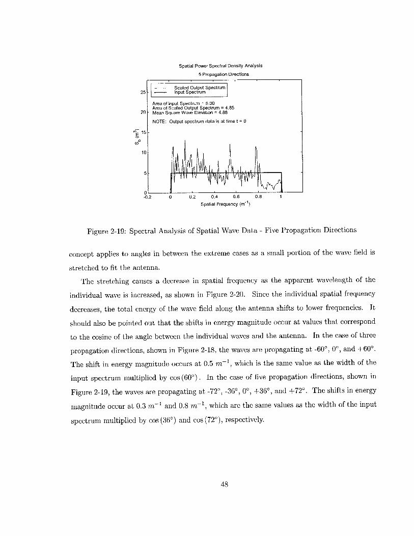
Figure 2-19: Spectral Analysis of Spatial Wave Data - Five Propagation Directions

concept applies to angles in between the extreme cases as a small portion of the wave field is

stretched to fit the antenna.

The stretching causes a decrease in spatial frequency as the apparent wavelength of the

individual wave is increased, as shown in Figure 2-20. Since the individual spatial frequency

decreases, the total energy of the wave field along the antenna shifts to lower frequencies. It

should also be pointed out that the shifts in energy magnitude occur at values that correspond

to the cosine of the angle between the individual waves and the antenna. In the case of three

propagation directions, shown in Figure 2-18, the waves are propagating at -60', 00, and +60'.

The shift in energy magnitude occurs at 0.5 m-1, which is the same value as the width of the

input spectrum multiplied by cos (600) . In the case of five propagation directions, shown in

Figure 2-19, the waves are propagating at -72', -36', 0', +360 , and +720. The shifts in energy

magnitude occur at 0.3 m- 1 and 0.8 m-1, which are the same values as the width of the input

spectrum multiplied by cos (360) and cos (720), respectively.

48

Figure 2-20: Spatial Frequency Stretching

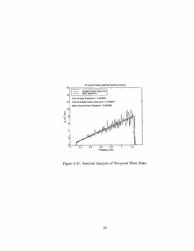
2.5.4 Temporal Spectral Analysis

By sampling the wave record temporally for sea surface elevation, one can determine the tem-

poral power spectral density curve of the modeled wave field. By comparing the resultant

spectral density curve to the desired spectral density curve, a verification of the model's wave

field generation method can be conducted. Figure 2-21 shows the temporal spectral analysis

of a model generated wave field. The resultant energy density spectrum closely resembles the

desired input spectrum and there is good agreement amongst the values representing the area

under the input spectrum, the area under the output spectrum, and the mean square wave

elevation of the modeled wave field.

49

16

14

1

U>

Temporal Power Spectral Density Analysis

Scaled Output Spectrum- Input Spectrum

0 0.2 0.4 0.6 0.8Frequency (Hz)

1 1.2

Figure 2-21: Spectral Analysis of Temporal Wave Data

50

Area of Input Spectrum = 5.0000002 - Area of Scaled Output Spectrum = 4.960691

Mean Square Wave Elevation = 5.005589

0

8-

6-

4-

2-

n

1

Chapter 3

Antenna Model Development

3.1 Coordinate System Description

The coordinate system adopted for the model is a three-dimensional system whose origin trans-

lates in the antenna tow direction at the antenna tow speed U, which is defined to be positive.

The origin of the antenna is defined to be the trailing point of the antenna. The waves travel

in the positive x direction, all at varying angles, but always from left to right in the positive x

direction. Figure 3-1 depicts the coordinate system in the x-z plane as well as the basic antenna

configuration. The antenna tow angle, 0, is the angle measured from the antenna to the prin-

cipal axis of wave propagation. It is defined to be 0' when pointing in the positive x direction

and 1800 when pointing in the negative x direction. The model allows the user to select any

tow angle between and including 0' and 180'. Due to port and starboard symmetry of the

anntena, the behavior of the antenna for the angles 180' to 3600 is identical to the behavior

of the antenna for the angles 00 to 1800. Figure 3-2 depicts the coordinate system in the x-y

plane as well as the antenna tow direction.

The equations listed in Table 2.1 apply to a stationary coordinate system. The transforma-

tion to a moving coordinate system employs the following relationship

x' = x + Ut (3.1)

where

51

Direction ofWave Propagation

x Tow SpeedU

Tow Point

Figure 3-1: Coordinate System:

Y

AntennaTow

Direction

HeadSeas

Figure 3-2: Coordinate System:

X-Z Plane

10X FollowingSeas

X-Y Plane

52

z

Drogue tenna

*** t 0,

X' is the earth-fixed, stationary, coordinate system

x is the moving coordinate system whose origin translates with velocity U , as shown in

Figures 3-1 and 3-2.

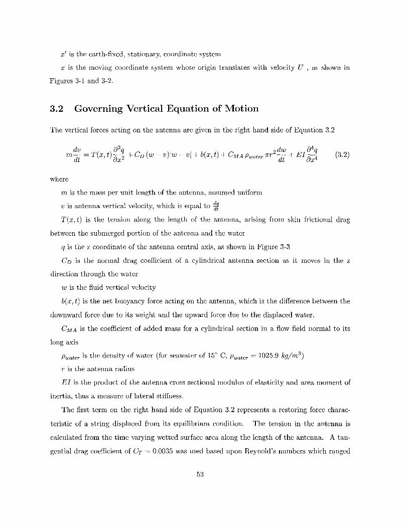
3.2 Governing Vertical Equation of Motion

The vertical forces acting on the antenna are given in the right hand side of Equation 3.2

dv _2_ 2 dw ___

m = T(x, t) + CD (w - v) w-vI b(x, t) + CMA Pwater T 2 2 + EI (3.2)dt Ox 2 d O 0x 4

where

m is the mass per unit length of the antenna, assumed uniform

v is antenna vertical velocity, which is equal to ddt

T(x, t) is the tension along the length of the antenna, arising from skin frictional drag

between the submerged portion of the antenna and the water

q is the z coordinate of the antenna central axis, as shown in Figure 3-3

CD is the normal drag coefficient of a cylindrical antenna section as it moves in the z

direction through the water

w is the fluid vertical velocity

b(x, t) is the net buoyancy force acting on the antenna, which is the difference between the

downward force due to its weight and the upward force due to the displaced water.

CMA is the coefficient of added mass for a cylindrical section in a flow field normal to its

long axis

Pwater is the density of water (for seawater of 150 C, Pwater = 1025.9 kg/m 3 )

r is the antenna radius

EI is the product of the antenna cross sectional modulus of elasticity and area moment of

inertia, thus a measure of lateral stiffness.

The first term on the right hand side of Equation 3.2 represents a restoring force charac-

teristic of a string displaced from its equilibrium condition. The tension in the antenna is

calculated from the time varying wetted surface area along the length of the antenna. A tan-

gential drag coefficient of CT = 0.0035 was used based upon Reynold's numbers which ranged

53

z

Sea Elevation Antenna Elevation

h q

Relative Antenna Elevation

y = q - h

Figure 3-3: Antenna and Sea Surface Elevation Variables

from 32,940 to 592,900 for speed/diameter combinations of 3 knots/1 inch to 9 knots/6 inches,

respectively. [1] The second term represents the normal drag force a cylindrical element would

experience as it is moved through the fluid with its long axis perpendicular to the direction of

motion. A value of CD = 1.0 was used, which assumes an infinite fluid domain. The fourth

term represents the added mass effect experienced by a cylindrical object as the fluid around it

is accelerating normal to the long axis of the cylinder. A value of CMA = 1.0 was used, which

is consistent with standard fluid dynamic texts assuming an infinite fluid domain. [6] The final

term represents the restoring force due to the stiffness of the material, and its distribution with

respect to the neutral axis. Initial design options have the lateral stiffness ranging from 300 to

21400 Pa-m

It is recognized that some of these forces have been approximated, namely in that the values

quoted above are for CD and CMA in an infinite fluid domain. The antenna operates in close

proximity to the free surface, and occasionally portions rise completely above the surface of

the water. A rigorous treatment of the behavior of CD and CMA near the free surface was not

attempted. Rather, a straightforward linear approximation was employed which varied the

coefficients CD and CMA from their infinite fluid domain values when the antenna axis was at

54

Conductor: Antenna Element:Isometric View Section View

Figure 3-4: Antenna Element Description

a depth of r, just submerged, to a value of zero when the antenna axis was at a height of r,

just breaking out of the water. This dependence of CD and CMA on relative antenna depth, y,

is shown in Equations 3.3 and 3.4, which only apply to the partially submerged case.

CD(Y) = -Y- 1) (3-3)

CMA(Y) = MAInfinite + (34)+r 2' 34

3.3 Antenna Modeling Methods

3.3.1 Discretization

The antenna, of length L, is subdivided first into lengths of the physical radio antenna elements.

These antenna elements, designed at Lincoln Laboratory, are called "jelly roll" antennas because

they are a conducting sheet rolled up about 11 times. A graphical description of the antenna

element is shown in Figure 3-4. The element length is designated Lejem. This first level of

subdivision is not only logical, but necessary for the exposure statistics calculated by the model.

55

Element' Length

Leiem

4Element Length

Lelem

I I I

L = Neiem Lelem

Leiem = M As

Mesh' Length 4

As

Figure 3-5: Antenna and Antenna Element Description

As it turns out, this type of antenna element performs well as long as it has some small amount,

on the order of 1 mm, of its outer housing diameter exposed along its entire length. But if

the element becomes covered by even a small amount of water at any point along its length,

antenna performance drops dramatically. Thus it is necessary to monitor numerous points

within each element to determine whether a given element is exposed or not. This leads to

the final level of antenna subdivision: each element is meshed into some integer number M of

sections with length As. The subdivision process is shown in Figure 3-5.

An interesting feature of the models which calculate the sea elevation and fluid velocities

by Fast Fourier Transforms (FFTs) is that the frequency meshing (Aw) of the spectral energy

density function S(w), is now related to the spatial meshing (Ax) of the sea, and thus the

spatial meshing of the antenna (As). This means that there is an extra constraint to consider

56

AntennaLength

L

Nelem= 7

M=6

I - I - I I I I 1 7 1

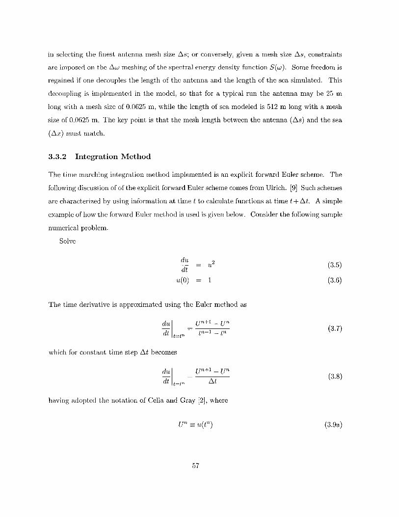
in selecting the finest antenna mesh size As; or conversely, given a mesh size As, constraints

are imposed on the Aw meshing of the spectral energy density function S(w). Some freedom is

regained if one decouples the length of the antenna and the length of the sea simulated. This

decoupling is implemented in the model, so that for a typical run the antenna may be 25 m

long with a mesh size of 0.0625 m, while the length of sea modeled is 512 m long with a mesh

size of 0.0625 m. The key point is that the mesh length between the antenna (As) and the sea

(Ax) must match.

3.3.2 Integration Method

The time marching integration method implemented is an explicit forward Euler scheme. The

following discussion of of the explicit forward Euler scheme comes from Ulrich. [9] Such schemes

are characterized by using information at time t to calculate functions at time t+ At. A simple

example of how the forward Euler method is used is given below. Consider the following sample

numerical problem.

Solve

= U2 (3.5)

u(0) = 1 (3.6)

The time derivative is approximated using the Euler method as

du Un+1 - Un (37)dt ti' n+1 - tn 37

which for constant time step At becomes

du Un+1 - U(- -= A (3.8)dt t.t At

having adopted the notation of Celia and Gray [2], where

U" = U(tn) (3.9a)

57

and t" is the nth time step. Then the solution proceeds step by step, beginning with the initial

value of u given in Equation 3.6

= U(0)2 = 1 (3.10)dt t=O

then solving Equation 3.8 for U'+ 1 we obtain

U = UO + At du (3.11)dt ltO

With the value of a now known at time t (U1 ), we can calculate

du (U1) 2 (3.12)

d t=1

and

u2 = u + At (3.13)dt t~t

In like manner, we move forward in time to calculate any desired U'. Numerical experi-

mentation was used to determine the appropriate time step size which produced acceptable

results.

The spatial derivatives (dq) used in the model are classified as centered finite-divided-

difference formulas. [3] Thus the antenna algorithm can be classified as a forward time, centered

space (FTCS) method.

3.3.3 Boundary Conditions

The boundary conditions imposed on the antenna endpoints are given in Equations 3.14 and

3.15 as

q(0) = h(0) (3.14)

q(L) = h(L) (3.15)

58

That is, the antenna follows the sea surface at its endpoints. This is envisioned to be accom-

plished at the trailing end by a drogue having positive buoyancy, and at the tow point by one

of several options. These options include

" a dynamic lifting body

" a surface following buoy

" a leader of positive buoyancy

" some combination of the above features.

3.3.4 Initial Conditions

The antenna simulation begins at t = 0 with

q(x)

dq(x)

dt

h(x)

dh(x)dt

(3.16)

(3.17)

that is, the antenna is placed at the sea surface, and given an initial vertical velocity matching

that of the sea surface.

59

Chapter 4

Modeling Results

4.1 Exposure Statistics

4.1.1 Definition of Exposure

The primary goal of the modeling effort was to predict exposure statistics as various design

and operational parameters were varied; therefore, it is necessary to define exposure before

proceeding on to the exposure statistics results. The overall exposure of the antenna is driven

by the exposure of individual antenna elements, so the determination of an exposed, or receiving,

antenna element must be addressed. The experimentally observed performance characteristics

of the "jelly roll" antenna elements led to the following definition of exposure. It was found that

for a level element in calm water, the antenna gain is stable right up to the point at which the

outer skin becomes completely submerged. It was also found that if any portion of the outer

skin was completely covered by water then the gain of the element suffered drastically. Thus an

exposed element was defined to be one which was exposed by some small threshold height, set

to four percent of Diameter for all simulations, at every point along the length of the element.

In a discrete computer model some approximation is necessary with regard to every point along

the length of the element. Thus each antenna element was divided into smaller segments for

analysis. Typical designs considered had an element length of 0.5 m and were further divided,

or oversampled, at M = 8.

60

4.1.2 Statistics Calculated by the Model

The computer model was programmed to track three key statistics:

* average exposure - the average fraction of antenna elements exposed throughout the entire

duration of the simulation

" threshold met - the average fraction of the time that some specified number of antenna

elements, or more, were exposed

* average counterdetection length - the average length of the antenna where there is no

water touching the antenna.

In addition, a record is made at each sample time of the condition of every antenna element,

such that when the simulation is finished, an exposure matrix is available for further post-

processing. Examples of information which could be extracted from the exposure matrix

include

* average drop-out time of a specific element

* average spatial length of wave wash-overs

* histograms and standard deviations of the number of exposed elements

" exposure statistics for an array not fully populated (i.e., one could examine only the

columns which had antenna elements installed) .

Five output files are generated for each run of the computer model. These output files are

described in detail in Appendix A. The input parameters which are specified for each run of

the computer model are also described in detail in Appendix A.

In the exposure statistics results given below, each series of simulations is presented in the

following manner:

" a listing of the antenna and operational parameters input table used to generate the series

" a plot of the average fraction of elements exposed

61

. a brief discussion of the exposure plot.

It is important to realize that these plots represent averages in time and space. This is

necessary in order to display the results as functions of key antenna design and operational

parameters, which is most useful from a designer's viewpoint. From the output files, it is also

possible to analyze how the statistics vary as time progresses, or how the statistics vary along

the array from the tow point to the trailing end. Although there are a large number of possible

statistics that could be analyzed for an even larger number of design and operational param-

eter combinations, only one statistic is presented here for seven selected design or operational

parameters.

62

Table 4.1: Series 1

4.2 Results

4.2.1 Series 1: Statistics vs. Number of Propagation Directions

Input

The input parameters for Series 1: Statistics versus Number of Propagation Directions, are

given in Table 4.1. This is a measure of the fineness of the angular sea description. The

number of propagation directions used were 1, 5, 9, 13, 17, and 21. The tow angles used were

0, 45, 90, 135, and 180 degrees.

63

Parameter

DurationNelem

LantLeiem

DiameterEl

PantMUTow AngleHsDevelopmentSpectral Model

Spreading Function

NfreqNN

Description

60 sec7336.5 m0.5 m3.0 inches100 N-rn 2

408 kg/M 3

85.0 kts00 450 ,900 ,1350 ,1800

3.0 m1.0Bretschneidercos

2

2131,5,9,13,17,21

Input Parameters

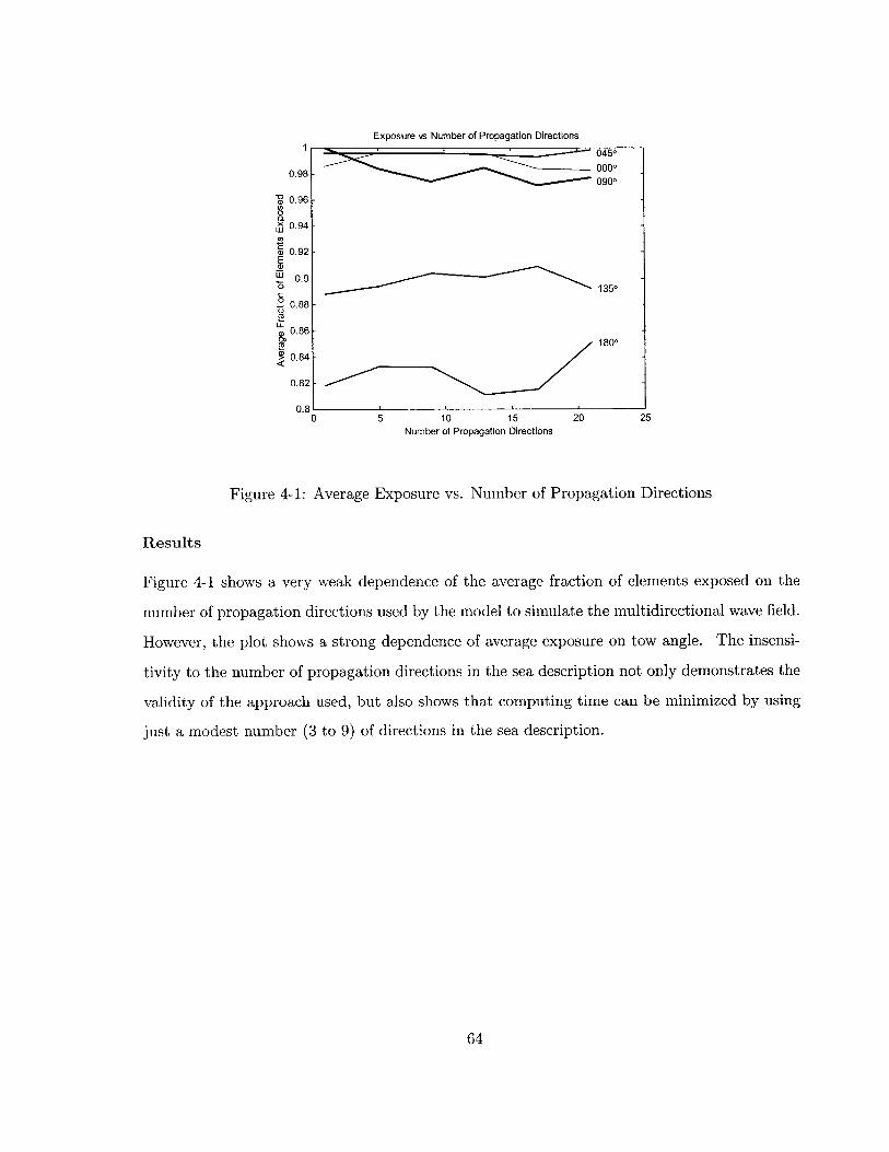
Exposure vs Number of Propagation Directions1 0450

0.98 -0000900

-O 0.96-0.901

0.94 -

a) 0.92-E

_W 0.9-o 1350

0.8

0.88

L ~,0.86-1800

S0.84

0.82

0.810 5 10 15 20 25

Number of Propagation Directions

Figure 4-1: Average Exposure vs. Number of Propagation Directions

Results

Figure 4-1 shows a very weak dependence of the average fraction of elements exposed on the

number of propagation directions used by the model to simulate the multidirectional wave field.

However, the plot shows a strong dependence of average exposure on tow angle. The insensi-

tivity to the number of propagation directions in the sea description not only demonstrates the

validity of the approach used, but also shows that computing time can be minimized by using

just a modest number (3 to 9) of directions in the sea description.

64

Parameter Description

Duration

Neiem

Lant

Leiem

DiameterEI

PantM

U

Tow Angle

HsDevelopment

Spectral Model

Spreading Function

NfreqNN

60 sec7336.5 m0.5 m

3.0 inches100 N-m2

408 kg/M 3

85.0 kts0 ,300,600,900,1200,1500,18003.0 m1.0Bretschneidercos

2

213

3

Table 4.2: Series 2 Input Parameters

4.2.2 Series 2: Statistics vs. Tow Angle

Input

The input parameters for Series 2: Statistics versus Tow Angle, are given in Table 4.2. The

tow angles used were 0, 30, 60, 90, 120, 150, and 180 degrees.

65

Parameter Description

Exposure \s Tow Angle

0 20 40 60 80 100 120Tow Angle (degrees)

140 160 180

Figure 4-2: Average Exposure vs. Tow Angle

Results

Figure 4-2 shows a rather weak dependence of the average fraction of elements exposed on the

tow angle from 0-90' (following seas); however, there is a very strong dependence on tow angle

from 90'-180' (head seas).

66

o 0.960.w

c 0.94a)Ea)W0.92

0

CU09

LCL

0.88

0.86

0.84

1

0.98


4.2.3 Series 3: Statistics vs. Sea Severity

Input

The input parameters for Series 3: Statistics versus Sea Severity, are given in Table 4.3. The

significant wave heights used were 0.5, 1.0, 1.5, 2.0, 2.5, and 3.0 meters. The tow angles used

were 0, 45, 90, 135, and 180 degrees.

67

Parameter

Duration

Neiem

LantLelem

DiameterEI

PantMUTow Angle

HSDevelopmentSpectral Model

Spreading Function

Nfreq

NN

Description

60 sec7336.5 m0.5 m3.0 inches100 N-m2

408 kg/M 3

85.0 kts

0 ,450 ,900 ,1350 ,18000.5,1.0,1.5,2.0,2.5,3.0 m

1.0Bretschneidercos

2

2133

Exposure vs Significant Wa\e Height

0 0.5 1 1.5 2Significant Wave Height (m)

2.5

Figure 4-3: Average Exposure vs. Sea Severity

Results

Figure 4-3 shows a rather weak dependence of the average fraction of elements exposed on the

significant wave height at all tow angles.

68

0C.wa,

E0)wI0C0

LL

0.951-

0.9 V

045009000000

1350

1800

0.853 3.5

1


4.2.4 Series 4: Statistics vs. Tow Speed

Input

The input parameters for Series 4: Statistics versus Tow Speed, are given in Table 4.4. The

tow speeds used were 3, 5, 7, and 9 knots. The tow angles used were 0, 45, 90, 135, and 180

degrees.

69

Parameter

DurationNeiemLant

Leiem

DiameterEI

PantM

U

Tow AngleHsDevelopmentSpectral Model

Spreading Function

NfreqNN

Description

60 sec7336.5 m0.5 m3.0 inches200 N-m2

408 kg/M 3

83,5,7,9 kts0 ,450,900,135 ,18003.0 m1.0Bretschneidercos

2

2133

Exposure vs Tow Speed

2 3 4 5 6 7Tow Speed (m/sec)

8 9 10

Figure 4-4: Average Exposure vs. Tow Speed

Results

Figure 4-4 demonstrates the effect that tow angle has on other parameters. In this instance,

increasing tow speed for tow angles greater than 900 (head seas) causes a decrease in exposure

fraction. While, for tow angles less than 900 (following seas), increasing tow speed causes an

increase in exposure fraction.

70

'0

0

CD

0C

0,

LL

0.95-

0.9-

0.85

0.8

0.75 -

0450............. 0 0 0 0

0900

1350

1800

0.7 - - -


4.2.5 Series 5: Statistics vs. Antenna Length

Input

The input parameters for Series 5: Statistics versus Antenna Length, are given in Table 4.5.

The antenna lengths used were 5, 15, 25, 60, and 100 meters. The tow angles used were 0, 45,

90, 135, and 180 degrees.

71

Parameter

Duration

NelemLant

Leiem

DiameterEl

PantM

U

Tow Angle

HsDevelopmentSpectral ModelSpreading Function

Nfreq

NN

Description

60 sec10,30,50,120,2005,15,25,60,100 m

0.5 m

3.0 inches200 N-m2

408 kg/M 3

85.0 kts0 ,450 ,900 ,1350 ,18003.0 m1.0Bretschneidercos

2

2133

Exposure vs Antenna Length

000009000450

-O 0.95-0 .0 .aw

Ca, 0.9-E

0

0 1350 10.85-

Li.CD

-M 1800S0.8

0 10 20 30 40 50 60 70 80 90 100 110Antenna Length (m)

Figure 4-5: Average Exposure vs. Antenna Length

Results

Figure 4-5 shows a very strong dependence of the average fraction of elements exposed on the

antenna length for lengths less than 25 meters. For lengths greater than 25 meters, there is

little or no dependence on antenna length.

72

1


4.2.6 Series 6: Statistics vs. Antenna Diameter

Input

The input parameters for Series 6: Statistics versus Antenna Diameter, are given in Table 4.6.

The antenna diameters used were 3 and 6 inches. The tow angles used were 0, 45, 90, 135,

and 180 degrees.

73

Parameter

Duration

NelemLantLeiemDiameter

EI

PantMUTow Angle

HSDevelopmentSpectral Model

Spreading Function

Nfreq

NN

Description

60 sec7336.5 m0.5 m3.0,6.0 inches200 N-m2408 kg/M 3

85.0 kts

0 ,450,900 ,135 ,18003.0 m1.0Bretschneidercos

2

2133

Exposure vs Antenna Diameter1-

0.98-

0.96-

S0.94 -w

0.92-E

0.9-0

c 0.88-

0.86-

2 0.84-

0.82-

0.8-

2. 5.5 6 6.5

Figure 4-6: Average Exposure vs. Antenna Diameter

Results

Figure 4-6 also demonstrates the influence that tow angle has on amplifying the effects of design

parameter changes. In all cases shown, the larger diameter antenna has an increased exposure

fraction, but the change is most significant for head seas cases.

74

3 3.5 4 4.5 5Antenna Diameter (m)

,uu

0900

1350

1800

5

Parameter

Duration

NelemLant

Leiem

DiameterEl

PantM

UTow Angle

HsDevelopmentSpectral Model

Spreading Function

Nfreq

NN


4.2.7 Series 7: Statistics vs. Antenna Density

Input

The input parameters for Series 7: Statistics versus Antenna Density, are given in Table 4.7.

The antenna densities used were 200, 300, 400, 500, and 600 kg/m 3 . The tow angles used were

0, 45, 90, 135, and 180 degrees.

75

Description

60 sec7336.5 m0.5 m3.0 inches200 N-m2

200,300,400,500,600 kg/m3

85.0 kts0 ,450 ,900 ,1350 ,18003.0 rn1.0Bretschneidercos

2

2133

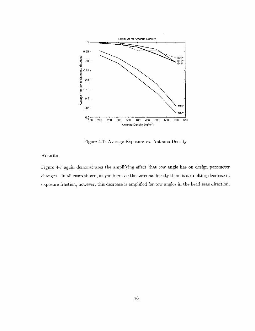
Exposure vs Antenna Density

000009000450

1350

1800

200 250 300 350 400 450 500

Antenna Density (kg/m3)

550 600 650

Figure 4-7: Average Exposure vs. Antenna Density

Results

Figure 4-7 again demonstrates the amplifying effect that tow angle has on design parameter

changes. In all cases shown, as you increase the antenna density there is a resulting decrease in

exposure fraction; however, this decrease is amplified for tow angles in the head seas direction.

76

0.95-

0.9 -0.

o 0.8-

LI)

a>

t0.7U-

0)

-W 0.7-

0.65

07-

50150

1

L

Chapter 5

Future Efforts

The combined Navy and DARPA Multi-element Buoyant Cable Antenna effort was funded

in FY 00 for 3 years. The demonstration phase culminated with a successful testing effort in

Hawaii in the Summer of 1999. Within FY 00, Lincoln Laboratory is scheduled to complete the

development and design of an antenna which can stand up to the rigors of an at sea deployment.

FY 01 will see the initial production of the deployable version with the goal of at sea submarine

testing during FY 02.

Work at MIT will continue to support the buoyant cable antenna effort. Another graduate

student, under the supervision of Professor Jerome Milgram, will continue and extend the

scope of the simulation effort. Areas which will be investigated to improve the capability of

the computer model include

" more detailed modeling of the hydrodynamics at the free surface

" higher order integration schemes

" addition of digital signal processors to improve computation speed

" validation against tow tank data

" validation against at-sea test data

" effects of roll for revised antenna elements whose performance depends on roll angle.

77

Appendix A

User's Guide to Proteus

A.1 Introduction

A.1.1 Contents of the User's Guide

The User's Guide is broken down into three sections:

" Introduction

" Input File

" Output Files.

Section A. 1 describes the contents of the user's guide and contains the procedures necessary

to obtain the results discussed in Section A.3. Section A.2 describes the Proteus input file line

by line and includes program features and limitations associated with each parameter. Section

A.3 briefly describes the contents of each of the five output files and the recommended methods

of viewing or extracting the information.

A.1.2 Analysis Procedure

Obtaining the Snapshot Output

1. Ensure that the input file, proteus_ input.txt, is located in the same directory as the

FORTRAN executable file, proteus.exe.

78

2. Modify the input file to reflect the conditions that the user wishes to analyze, using Section

A.2 as guidance for features and limitations. Ensure that the matlab_ output variable is

set to .TRUE.

3. Execute proteus. exe.

4. The snapshot output file (run_ id//'_mat') will be located in the same directory as the

executable file.

5. Ensure that the output file (run_ id//'_ mat') will be located in the same directory as

the Matlab function file, proteus_ mat.

6. At the Matlab command line type: clear; proteus_ mat('run_ id// mat').

Obtaining the Parameters and Results Summary




A.2 as guidance for features and limitations. Ensure that the run_ info variable is set to

.TRUE.


4. The parameters and results summary output file (run_ id//'_info.txt') will be located in

the same directory as the executable file.

5. The output file can be viewed with any standard text editor.

Obtaining the Exposure Data Matrix




A.2 as guidance for features and limitations. Ensure that the exp_ data variable is set to

.TRUE.

79


4. The exposure data matrix output file (run id//'_edm') will be located in the same

directory as the executable file.

5. The output file can be viewed with a user supplied Matlab® file or with a spreadsheet

application.

Obtaining Wave Data Temporal Spectrum Analysis

1. Ensure that the input file, proteus_ input. txt, is located in the same directory as the



A.2 as guidance for features and limitations. Ensure that the wave_ temporal variable is

set to .TRUE.

3. Execute proteus.exe.

4. The temporal wave data output file (run_ id//'_mat2') will be located in the same di-

rectory as the executable file.

5. Ensure that the output file (run_ id//'_mat2') will be located in the same directory as

the executable file, proteus_ mat2. exe.

6. Execute proteus_ mat2. exe. When the program prompts the user for filename, enter

run id/_ mat2.

7. Ensure that the output file (run_ id//'_mat2_proc') will be located in the same directory

as the Matlab function file, proteus_ mat2.

8. At the Matlab command line type: clear; proteus_ mat2('run_ id// mat2_ proc').

Obtaining Wave Data Spatial Spectrum Analysis



80


A.2 as guidance for features and limitations. Ensure that the wave_ spatial variable is

set to .TRUE.


4. The spatial wave data output file (run_ id//'_mat3') will be located in the same directory

as the executable file.

5. Ensure that the output file (runid//'_mat3') will be located in the same directory as

the executable file, proteus_ mat3. exe.

6. Execute proteus_ mat3. exe. When the program prompts the user for filename, enter

run_ id/_ mat3.

7. Ensure that the output file (run_ id//'_mat3_ proc') will be located in the same directory

as the Matlab function file, proteus_ mat3.

8. At the Matlab command line type: clear; proteus_ mat3('run id/ mat3_ proc').

A.2 Proteus Input File

A.2.1 Description of Features and Limitations

Header

The input file for Proteus is shown in Section A.2.2. The first 7 lines are for informational

purposes and have no effect on the program. However, note that all variables are given in SI

units and that there must be 7 lines prior to the first variable defined.

Run Identifier (run_ id)

The run_ id is an 8 character variable used to name the 5 output files. The 5 output files are

named

e run id//'_mat'

81

. run_ id//'_info.txt'

* run_ id//'_edm'

* run id//'_mat2'

" run_ id//'_ mat3'.

(The // represents FORTRAN90 string concatenation.) Output files are located in the local

directory from which the program is run. A sample pattern for run_ id is run_ id='15May_01'.

Characters which Matlab@ would interpret as operators (/, +, -, *, etc.) should be avoided in

run_ id if one of the Matlab output options is selected.

FFT Power of 2 (nnf)

The FFT algorithm is designed to operate on arrays which have an integer power of 2 elements.

nnf sets this power of 2, making

N sea = 2nnf (A.1)

where

N_sea is the number of sea frequency components and spatial locations.

The length of the sea surface modeled in the spatial domain is generally much larger than

the antenna length requires; however, the speed advantage of the FFT method more than

outweighs the penalty of carrying along the extra sea information.

Number of Antenna Elements (num_ of_ elem)

This is the number of physical antenna receiver elements in the array, assuming that

" the array is fully populated

* the elements have zero space between them.

Antenna Element Length (element_ length)

This is the length of each antenna element.

82

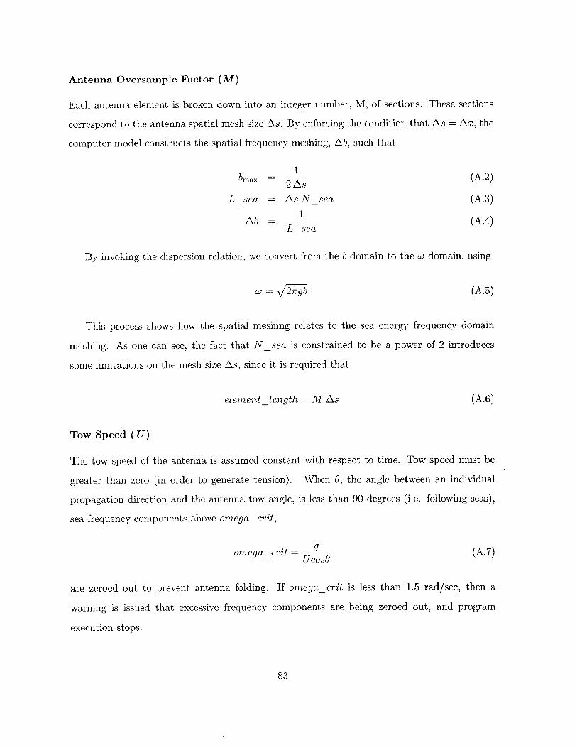
Antenna Oversample Factor (M)

Each antenna element is broken down into an integer number, M, of sections. These sections

correspond to the antenna spatial mesh size As. By enforcing the condition that As = Ax, the

computer model constructs the spatial frequency meshing, Ab, such that

1bmax (A.2)

2As

Lsea = As Nsea (A.3)

1Ab = (A.4)

L-sea

By invoking the dispersion relation, we convert from the b domain to the w domain, using

w = '27rg b (A.5)

This process shows how the spatial meshing relates to the sea energy frequency domain

meshing. As one can see, the fact that Nsea is constrained to be a power of 2 introduces

some limitations on the mesh size As, since it is required that

element_length = M As (A.6)

Tow Speed (U)

The tow speed of the antenna is assumed constant with respect to time. Tow speed must be

greater than zero (in order to generate tension). When 0, the angle between an individual

propagation direction and the antenna tow angle, is less than 90 degrees (i.e. following seas),

sea frequency components above omegacrit,

omega crit = 9 (A.7)

are zeroed out to prevent antenna folding. If omega_crit is less than 1.5 rad/sec, then a

warning is issued that excessive frequency components are being zeroed out, and program

execution stops.

83

Simulation Time (duration)

The total length of time simulated by the program.

Antenna Time Step Increment ( t_ incr)

The time step increment used in solving the antenna's governing equation. A typical value

for an antenna with no stiffness is 0.001 seconds. When stiffness is added, the time increment

should be reduced to 0.0001 seconds. In all cases, if the program stops executing due to a

run-time math error, the time increment should be made smaller to allow proper execution of

the program.

Snapshot Output Interval (pic_ time)

This variable allows the user to control the time interval between snapshots, which are recorded

to file run_ id//'_mat'. These snapshots record both the sea and antenna elevation data along

the entire length of the antenna, at a resolution of As.

Time of First Snapshot (tfirstpic)

The time to begin recording snapshots is user defined. This is useful to ignore transient behavior

at the start of the simulation, or to save only a representative sample at the end of a lengthy

simulation.

Statistics Output Interval (stat_ time)

This variable allows the user to control the time interval between exposure data matrix records,

which are recorded to file run_ id//'_edm'. Selection of an excessively small stat_ time results

in subsequent records containing essentially the same information, and contributes little to the

statistics of the sample.

Snapshot Output Option(matlab_ output)

The snapshot output file (run id//'_mat') is optional, since it does not contain any unique

statistical information, and requires a relatively large amount of disk space. The primary

84

benefit of examining the snapshot output file is to learn the physical behavior of the antenna in

a seaway. In addition, the output is useful to detect when the time step size is too small, which

is characterized by rapid unphysical antenna oscillations. matlab_ output=.TRUE. means that

snapshot output is enabled, .FALSE. means snapshot output is disabled.

Simulation Parameters and Results Summary Option (run_ info)

The simulation parameters and results summary file (run id//'_info.txt') is optional, but is

highly recommended as it contains all of the pertinent inputs and results of the simulation.

run_ info=.TRUE. means that summary output is enabled, .FALSE. means summary output

is disabled.

Exposure Data Matrix Option (exp_ data)

The exposure data matrix file (run_ id//'_edm') is optional; since, it is needed only when

examining the exposure of individual elements rather than being concerned with the overall

exposure of the antenna. exp_ data=.TRUE. means that the exposure data matrix output is

enabled, .FALSE. means that the exposure data matrix output is disabled.

Temporal Wave Data Option (wave_ temporal)

The temporal wave data file (run_ id//'_mat2') is optional, since it is needed only when an-

alyzing the power spectrum of the modeled seas in time. It contains the wave elevation at a

single random point on the antenna in time. wave_ temporal=.TRUE. means that the temporal

wave data output is enabled, .FALSE. means that the temporal wave data output is disabled.

Spatial Wave Data Option (wave_ spatial)

The spatial wave data file (run_ id//'_mat3') is optional, since it is needed only when analyzing

the power spectrum of modeled seas along the antenna. It contains the wave elevation at every

point on the antenna for the time = 0.0 seconds. wave_ spatial=.TRUE. means that the spatial

wave data output is enabled, .FALSE. means that the spatial wave data output is disabled.

85

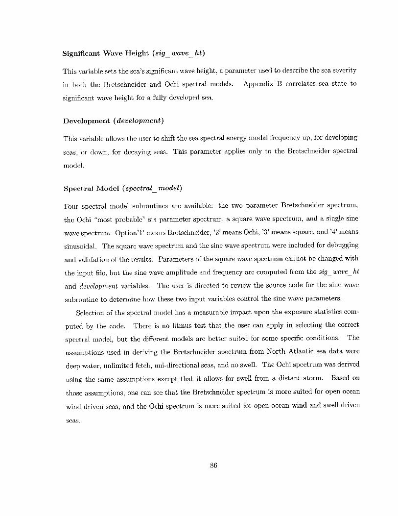
Significant Wave Height (sig_ wave_ ht)

This variable sets the sea's significant wave height, a parameter used to describe the sea severity

in both the Bretschneider and Ochi spectral models. Appendix B correlates sea state to

significant wave height for a fully developed sea.

Development (development)

This variable allows the user to shift the sea spectral energy modal frequency up, for developing

seas, or down, for decaying seas. This parameter applies only to the Bretschneider spectral

model.

Spectral Model (spectral_ model)

Four spectral model subroutines are available: the two parameter Bretschneider spectrum,

the Ochi "most probable" six parameter spectrum, a square wave spectrum, and a single sine

wave spectrum. Option'1' means Bretschneider, '2' means Ochi, '3' means square, and '4' means

sinusoidal. The square wave spectrum and the sine wave spectrum were included for debugging

and validation of the results. Parameters of the square wave spectrum cannot be changed with

the input file, but the sine wave amplitude and frequency are computed from the sig_ wave_ ht

and development variables. The user is directed to review the source code for the sine wave

subroutine to determine how these two input variables control the sine wave parameters.

Selection of the spectral model has a measurable impact upon the exposure statistics com-

puted by the code. There is no litmus test that the user can apply in selecting the correct

spectral model, but the different models are better suited for some specific conditions. The

assumptions used in deriving the Bretschneider spectrum from North Atlantic sea data were

deep water, unlimited fetch, uni-directional seas, and no swell. The Ochi spectrum was derived

using the same assumptions except that it allows for swell from a distant storm. Based on

those assumptions, one can see that the Bretschneider spectrum is more suited for open ocean

wind driven seas, and the Ochi spectrum is more suited for open ocean wind and swell driven

seas.

86

Directional Spreading Function (spreading_func)

This allows the user to select the directional spreading function to apply to the power spectra

to obtain the desired wave field. Two directional spreading functions are available: cos2 O and

cos 4 0. Option '1' means cos 2 0 and option '2' means cos 40.

Number of Propagation Directions (NN)

This allows the user to select the number of discrete unidirectional waves which will combine

to form the multidirectional sea surface. A larger number of directions will result in more

realistic sea spectra but at the expense of computation time. It is recommended that the user

experiment with the number of propagation directions until the simulation results converge.

Trapezoidal Integration Convergence Factor (epsilon)

This refers to the convergence factor of the trapezoidal integration that is needed to calculate

the integral of the directional spreading function. A typical value is le- 3 .

Antenna Tow Angle (tow_ angle)

Antenna tow angle with respect to the primary axis of propagation. A tow angle of 0 degrees

represents following seas, 90 degrees represents beam seas, and 180 degrees represents head

seas.

Antenna Diameter (diam_ antenna)

This is the outer diameter of the hose-like structure encasing the antenna. Element performance

(gain) is controlled by whether this outer diameter is submerged; the diameter of the inner

conducting slot antenna affects the rotational invariance of the element, and the maximum

theoretical gain of a fully exposed element.

Water Density (rho_ water)

Water density in which the antenna operates.

87

Drogue Size (drog_ area)

The drogue frontal area (in m2 ) determines the tension at the trailing end of the antenna,

according to

1T =-pwater U 2 drog_areaCDn (A.8)

2

A typical value is 0.01 m2 .

Normal Drag Coefficient (CD_ n)

This represents the drag coefficient for a cylinder in cross flow. A constant value of 1.0 has

been assumed.

Tangential Drag Coefficient (CD_ t)

This is the skin friction associated with flow along the long axis of the antenna. A relatively

smooth outer surface has been assumed in choosing this value, which has been assumed constant.

A typical value is 0.0035.

Antenna Density (rhoantenna)

The average antenna density, which is assumed to be constant over the entire array. This is

an approximation in that the antenna has slightly higher density at the actual element, and

slightly lower density between elements.

Antenna Lateral Stiffness (flex stiff_ coeff)

This variable represents the resistance of the antenna to bending, and is given by

flex stif f _coeff = El (A.9)

where

E is the modulus of elasticity

I is the area moment of inertia.

88

.04

Waterline

1.00

Figure A-1: Sample Threshold Antenna Exposure of 0.04

Added Mass Coefficient (C_ m)

The added mass coefficient for a cylinder in cross flow has been set to 1.0.

Maximum Number of Samples (max_ num_ of_ samples)

This refers to the maximum number of "snapshots" taken for the Matlab viewer, or the

exposure data matrix. max_ num_ of samples is used to dynamically allocate array storage for

variables which are sampled periodically in time.

Threshold Antenna Exposure (reqd_ ant_ exposure)

As mentioned earlier, the antenna gain remains steady until the element just becomes sub-

merged. In order to capture this performance, and introduce margin for capillary waves not

modeled, the parameter reqd_ ant_ exposure has been defined. The reqd_ ant_ exposure is the

height above the water which must be maintained by the antenna to be considered exposed.

The reqd ant_ exposure is given as a fraction of the antenna diameter. See Figure A-1 for a

diagram representing an antenna diameter of 1.0 and a reqd_ ant_ exposure of 0.04.

89

Threshold Number of Elements (num_ of elem_ thresh)

This variable allows the user to specify the lowest number of exposed antenna elements necessary

to achieve the desired design antenna array gain. At each stat_ time, the number of exposed

elements is compared to num_ of elem_ thresh; the result (a "1" when the threshold is met,

"0" otherwise) is found in the summary output file, run_ id//'_info.txt', along with any other

variables tracked over the course of the simulation. Currently, the variables tracked over time

are

" tow point tension (tow- tension( ))

" number of elements exposed (is_ exposed( ,

" threshold met (thresh_ met: "0" or "1", as above)

" counterdetection length (length_ totally_ exposed( )).

90

A.2.2 Sample Input File

Input File for proteus Simulation Program

SI units throughout; useful conversions follow

1 inch = 0.0254 in

1 foot = 0.3048 in

1 knot = 0.5144 m/s

runid

nnf

numof_ ele

element length

M

U

duration

tIincr

pic time

t first pic

stat time

matlab output

run info

expdata

wavetemporal

wave-spatial

sigwaveht

development

spectral_ model

spreading_ func

NN

epsilon

tow angle

diam _antenna

rho water

drog area

CD n

CDt

rhoantenna

flex_ stiff_ coeff

Cm

max _num ofsamples

reqd ant exposure

num of elem thresh

8 characters long

# of components. N-sea=2**nnf

# of actual slotted antenna elements

physical slotted antenna length (in)

# of mesh points/element length

tow speed (use POSITIVE #) (m/s)

total simulated run time (sec)

time step increment used for antenna calculations

snapshot interval for Matlab viewer (sec)

time of first snapshot (sec)

statistics interval (sec)

TRUE: A file is created that contains wave and antenna data

TRUE: A file is created that contains a summary of run parameters and results

TRUE: A file is created that contains the exposure data matrix

TRUE: A file is created that contains temporal wave elevation at a single point

TRUE: A file is created that contains spatial wave elevation at time=0

significant wave height (i)

modal frequency shift factor (used only for spectral model 1)

1=Bretschneider; 2=Ochi; 3=square; 4=sine

directional spreading function: 1=cos^2; 2=cos^4

Number of propagation directions (must be odd number)

Convergence factor for trapezoidal integration

Tow angle relative to primary axis of propagation (0-180 degrees)(0 following,180 head)

Antenna outer diameter (meters)

density of seawater (kg/m^3)

drogue area normal to fluid flow (m^2)

normal flow drag coefficient for a cylinder

antenna/fluid tangential drag coefficient

antenna density (kg/i^3)

lateral bending stiffness of antenna (Pa m^4) El

added mass coefficient for a cylinder

upper limit on # of samples in time domain

threshold amount of vertical exposure necess for reception (% of antenna diameter)

threshold # of elements required to achieve necessary gain

A.3 Output Files

A.3.1 Snapshot Output File (run_ id//'_mat')

File Description

This file provides:

91

15May_02

13

60

0.5

8

3.0

30.0

.001

0.2

0.0

0.1

.FALSE.

.TRUE.

.FALSE.

.FALSE.

.FALSE.

3.0

1.0

le-3

180.0

0.0762

1025.9

0.01

1.0

0.0035

408.0

100.0

1.0

1000

0.04

30

Run ID: 24May-01Sea Data For Time 0.00 sec

0 5 10 15Antenna Position (m)

3

2.5

2

1.5

1

0.5

0

-0.5

-1

-1.5

-2

Figure A-2: Sample Output of Snapshot Output File

" a time history of sea elevation along the antenna

" a time history of vertical, longitudinal, and transverse sea velocities along the antenna

" a time history of vertical antenna position

" antenna parameters necessary for the Matlab® function file.

This file is intended to be viewed with the Matlab function file, proteus_ mat.

Sample Output

A sample output of the Matlab function file proteus_ mat is shown in Figure A-2

A.3.2 Simulation Parameters and Results File (runid//'_info.txt')

File Description

This file provides:

e a complete listing of antenna parameters

92

20 25 30

Q)E

9 a complete listing sea spectra parameters

* a summary of exposure and antenna performance statistics.

This file is intended to be viewed with any standard text editor.

Sample Output

Summary of Parameters and Results

General Information

Run ID = 24May_01

Parameter and Result Summary File = 24May _01 _info.txt

Wave and Antenna Data File = 24May 01 mat

Start Date/Time 05/12/2000 07:22:31

End Date/Time 05/12/2000 07:41:07

Elapsed Computational Time = 1115.56 seconds

Simulated Analysis Time = 30.00 seconds

Antenna Parameters

Number of Antenna Elements = 60

Length of Antenna Element = 0.50 meters

Total Antenna Length = 30.00 meters

Antenna Diameter = 0.0762 meters

Lateral Bending Stiffness = 50.00 N-m^2

Antenna Density = 408.00 kg/m^3

Drogue Area Normal to Fluid Flow = 0.0100 m^2

Normal Flow Drag Coefficient for a Cylinder = 1.000000

Tangential Drag Coefficient = 0.003500

Coefficient of Added Mass for a Cylinder = 1.000000

93

Number of Mesh Points Per Element = 8

Tow Speed = 2.50 m/sec

Tow Angle = 180.0 degrees

Time Increment for Antenna Related Calculations 0.00010 seconds

Sea Spectra Parameters

Spectral Model = Bretschneider

Directional Spreading Function = cos^2

Development Factor = 1.00

Significant Wave Height = 3.00 meters

Minimum Cutoff Frequency = 0.35 radians/sec

Maximum Cutoff Frequency = 22.21 radians/sec

Length of Seas Modeled = 512.0 meters

Number of Spatial Sea Domain Mesh Points = 2^13

Number of Propagation Directions = 3

Seawater Density = 1025.90 kg/m^3

Time Increment for Sea Spectra Related Calculations 0.02125 seconds

Number of Antenna Time Increments Between Sea Spectra Calculations 212

Simulation Results

Maximum Tow Tension 116.4 N

Minimum Tow Tension = 24.3 N

Stretched Antenna Length = 30.2 meters

Antenna Strain = .005

Statistics Sampling Interval = 0.100 seconds

Number of Samples Observed for Statistics = 301

Average Fraction of Antenna Exposed = 0.895

Vertical Antenna Exposure Necessary to Receive = 4.0 percent of diameter

94

Number of Antenna Elements Required to be Exposed 30 / 60

Time That Number of Required Elements are Exposed 100.0 percent

Average Detection Length = 1.95 meters

A.3.3 Exposure Data Matrix File (run_ id//'_edm')

File Description

This file provides:

" the raw exposure data information for each antenna element at each time sampled

* the spatial position of all elements.

This allows one to analyze statistics across time or space. This file can be viewed with a

user supplied Matlab® file or with a spreadsheet application.

Sample Output

time spatial position / exposure status

0.00000

0.09900

0.19800

0.29700

0.39600

30.00000 29.50000 29.00000 28.50000 28.00000

0

0

0

A.3.4 Temporal Wave Data File (run id//'_mat2')

File Description

This file provides:

95

E3

16

14

12

10

8

6

4

2

0

Power Spectral Density Comparison for Data Run <17May-02>

-__ Scaled Output Spectrum- Input Spectrum

0 0.2 0.4 0.6 0.8frequency (Hz)

1 1.2

Figure A-3: Sample Output of Temporal Wave Data Analysis

" a time history of the wave elevation at a single random point on the antenna

" antenna parameters necessary for the Matlab function file.

This allows one to analyze the power spectrum of the modeled seas in time. It is intended

to be processed with the FORTRAN executable file, proteus_ mat2.exe, then viewed with the

Matlab® function file, proteus_ mat2.

Sample Output

A sample output of the Matlab® function file proteus_ mat2 is shown in Figure A-3.

A.3.5 Spatial Wave Data File (run id//'_mat3')

File Description

This file provides:

" the wave elevation at every point on the antenna at time = 0.0 seconds

" antenna parameters necessary for the Matlab® function file.

96

Area of Input Spectrum = 5.000000

Area of Unscaled Output Spectrum (Not Shown) = 0.056341

L/2k Scaling Factor = 86.84

Area of Scaled Output Spectrum = 4.892339

Number of data points per segment = 4096

Number of non-overlapping data segments = 2

Total Number of data points = 819

-

16

14

1:

1'

E

Cl)

Power Spectral Density Comparison for Data Run <17May-01>

-__ Scaled Output Spectrum-- Input Spectrum

-0.2 0 0.2 0.4 0.6 0.8 1

spatial frequency (m1)

Figure A-4: Sample Output of Spatial Wave Data Analysis

This allows one to analyze the power spectrum of the modeled seas in space. It is intended

to be processed with the FORTRAN executable file, proteus_ mat3. exe, then viewed with the

Matlab function file, proteus_ mat3.

Sample Output

A sample output of the Matlab@ function file proteus_ mat3 is shown in Figure A-4.

97

Area of Input Spectrum = 5.0000002 - Area of Unscaled Output Spectrum (Not Shown) = 0.075695

L/2k Scaling Factor = 64.00Area of Scaled Output Spectrum = 4.844453

0- Number of data points per segment = 1024Number of non-omedapping data segments = 8Total Number of data points = 8192

8 NOTE: Output spectrum data is at tim t = 0

6-

4-

2-

pi

Appendix B

Sea State Correlation Data

98

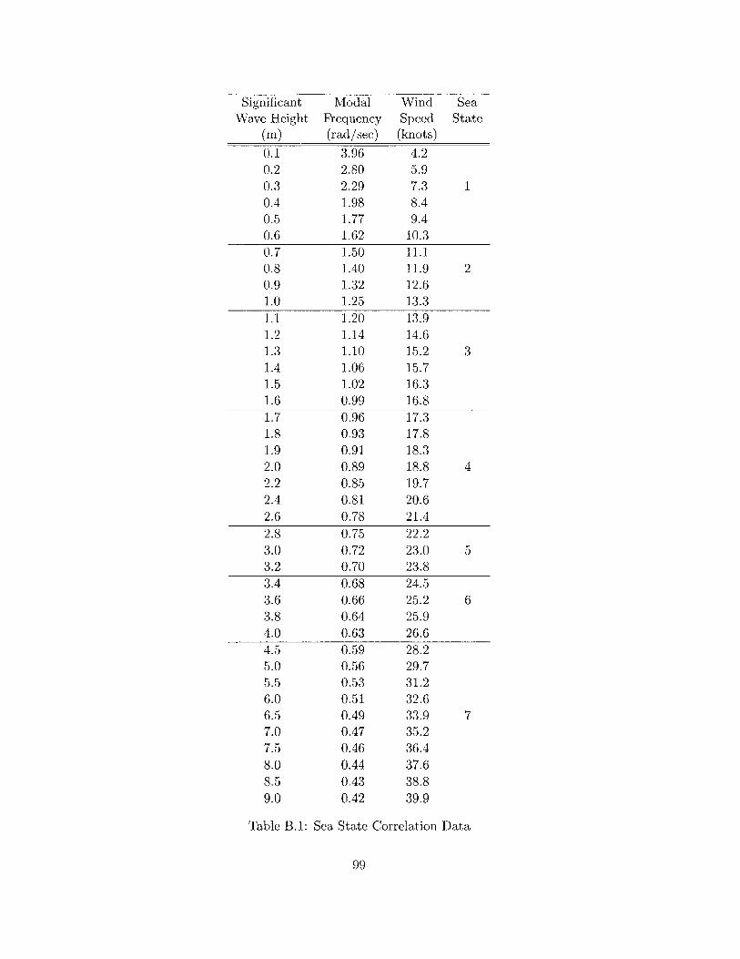
Table B.1: Sea State Correlation Data

99

SeaState

1

SignificantWave Height

(m)0.10.20.30.40.50.60.70.80.91.01.11.21.31.41.51.61.71.81.92.02.22.42.62.83.03.23.43.63.84.0

4.55.05.56.06.57.07.58.08.59.0

ModalFrequency

(rad/sec)3.962.802.291.981.771.621.501.401.321.251.201.141.101.061.020.990.960.930.910.890.850.810.780.750.720.700.680.660.640.630.590.560.530.510.490.470.460.440.430.42

WindSpeed

(knots)

4.25.97.38.49.4

10.311.111.912.613.313.914.615.215.716.316.817.317.818.318.819.720.621.422.223.023.824.525.225.926.628.229.731.232.633.935.236.437.638.839.9

7

2

3

4

5

6

Bibliography

[1] Berteaux, H. 0. Buoy Engineering. New York: John Wiley and Sons, Inc., 1976.

[2] Celia, M. A. and W. G. Gray. Numerical Methods for Differential Equations. Englewood

Cliffs, NewJersey: Prentice Hall, 1992.

[3] Chapra, Steven C. and Raymond P. Canale. Numerical Methods for Engineers (Second

Edition). New York: McGraw-Hill Publishing Company, 1988.

[4] Faltinsen, 0. M. Sea Loads on Ships and Offshore Structures. Cambridge Ocean Technology

Series - Volume One, United Kingdom: Cambridge University Press, 1990.

[5] Massel, Stanislaw R. Ocean Surface Waves: Their Physics and Prediction. Advanced

Series on Ocean Engineering - Volume Eleven, Singapore: World Scientific Publishing,

1996.

[6] Newman, John N. Marine Hydrodynamics. Cambridge, Massachusetts: MIT Press, 1977.

[7] Ochi, Michel K. Ocean Waves. Cambridge Ocean Technology Series - Volume Six, United

Kingdom: Cambridge University Press, 1998.

[8] Triantafyllou, M.S. and C. Chryssostomidis. Environment Description, Force Prediction

and Statistics for Design Applications in Ocean Engineering. Cambridge, MA: Department

of Ocean Engineering, Massachusetts Institute of Technology, 1980.

[9] Ulrich, Gary A., "Computer Model for a Towed Submarine Communication Antenna."

Naval Engineer thesis, Massachusetts Institute of Technology, Cambridge, Massachusetts,

1999.

100

[10] Ulrich, Gary A., "Source Code for a Computer Model for a Towed Submarine Communica-

tion Antenna." Massachusetts Institute of Technology, Department of Ocean Engineering,

Report 99-1, May 1999.

101

Hydrodynamic Modeling of Towed Buoyant Submarine ...

Documents

Transcript of Hydrodynamic Modeling of Towed Buoyant Submarine ...