Wind Forced Upwelling Over High Latitude Submarine Canyons

Wind Forced Upwelling Over High Latitude Submarine

Canyons: A Numerical Modeling Study

By

Hank Statscewich

A thesis submitted to the

Graduate School – New Brunswick

Rutgers, The State University of New Jersey

In partial fulfillment of the requirements

for the degree of

Master of Science

Graduate Program in Oceanography

written under the direction of

Professor Scott M. Glenn

And approved by

________________________________________________

________________________________________________

________________________________________________

________________________________________________

New Brunswick, New Jersey

January 2014

ii

ABSTRACT OF THE DISSERTATION

Wind-‐Forced Upwelling Over High Latitude Submarine Canyons: A Numerical

Modeling Study

By HANK STATSCEWICH

Dissertation Director:

Dr. Scott M. Glenn

Analytical and numerical models of circulation over submarine canyons are

presented where parameters such as stratification and canyon geometric scale

closely mimic the Mackenzie Canyon located in the Beaufort Sea. The analytical

model represents the linear, inviscid dynamics that take place during a geostrophic

adjustment. The numerical model contains a full representation of the Navier-‐Stokes

equations and is forced by a wind stress. Comparisons between the analytical and

numerical simulations show that both models accurately represent simple coastal

flow patterns in the vicinity of a coastal canyon.

Numerical simulations of a wind forced upwelling event on a shelf with a

canyon and a shelf without a canyon differ drastically. For the shelf without a

canyon, upwelled waters are confined to within 5-‐6 km of the coast and a uniform

along-‐shore coastal jet develops within 3 days of steady forcing. For the shelf with a

canyon, vertical velocities are much stronger within the canyon, and there is an

isolated region of upwelled waters that is confined to the coast along the axis of the

iii

canyon. Also, onshore trans ort is five times greater than offshore transport along

the axis of the canyon indicating that canyons facilitate cross-‐shelf mixing during

wind-‐forced upwelling events.

Simulations of the coastal ocean's response to passing frontal systems reach

an adjusted state after 5 days of continuous forcing. Alongshore transport

dominates the system with a minimal amount of net on shore or off shore transport

taking place in either of the model runs. Upon cessation of the winds, near-‐inertial

oscillations take place in both simulations.

iv

Acknowledgements

I would first like to thank Dr. Scott Glenn for serving as my advisor, and for

providing valuable insight during the course of my graduate education. Further, I

would like to express my greatest appreciation for Dr. Glenn's patience during our

many private discussions about my thesis which gave me inspiration and confidence

to continue at times when I felt the project was beyond the scope of my abilities.

I would like to thank Dr. Robert Chant and Dr. Dale Haidvogel for serving on

my thesis committee and for providing suggestions and criticisms of my thesis in an

objective and professional manner.

I would like to thank my family who have always supported me in my

academic pursuits, and stimulated my imagination at an early age by providing an

environment where creative thinking and inquiry were always encouraged.

I would like to thank Dr. Rich Styles, Dr. Heman Arango and Robert Cermak

for their comments, suggestions and support. Without these positive role models I

would have had a much harder time seeing the light at the end of the tunnel.

Finally, I would like to thank Marla Bryson whose personal support,

encouragement and positive outlook allowed me to persevere through the task of

completing this thesis.

v

Table of Contents

Abstract ................................................................................................................................... ii

Acknowledgements ......................................................................................................... iv

List of Tables ....................................................................................................................... vi

List of Figures .................................................................................................................... vii

1 Introduction .................................................................................................................... 1

1.1 Setting ......................................................................................................................................... 3

2 Literature Review ........................................................................................................ 9

3 Analytical Model ........................................................................................................ 15

3.1 Problem formulation for a 2-‐layer adjustment ......................................................... 15

3.2 Analytical Model Results ................................................................................................... 23

4 Problem Formulation for Numerical Simulations ............................... 29

5 Numerical Simulations .......................................................................................... 35

5.1 Boundary Condition Verification .................................................................................... 35

5.2 Shelf without canyon .......................................................................................................... 37

5.3 Shelf With Canyon ................................................................................................................ 41

5.4 Wave Generation .................................................................................................................. 45

6 Conclusion ..................................................................................................................... 50

REFERENCES ....................................................................................................................... 53

vi

LIST OF TABLES

Table 1: Model Parameters ................................................................................................................. 56

Table 2: Geometric Scales .................................................................................................................... 56

vii

LIST OF FIGURES

Figure 1 Map of the Arctic Ocean, the Mackenzie Bay Area is outlined in red. ............... 2

Figure 2 Bathymetric contours for the Mackenzie Bay study area. ..................................... 4

Figure 3 Cartoon of Ekman Surface layer transport. ................................................................. 6

Figure 4 Side view of the two level model. The variable for each level of the model is

indicated. ...................................................................................................................................... 15

Figure 5 The along-‐canyon structure of the initial sea surface and cross-‐canyon

velocity. ......................................................................................................................................... 16

Figure 6 The adjusted, steady state across canyon sea surface height , level 2 density

anomaly, level 1 velocities, and layer 2 velocities for a canyon that is 10 km

wide. ............................................................................................................................................... 24

Figure 7 The adjusted, steady state across canyon sea surface height, level 2 density


wide. ............................................................................................................................................... 25

Figure 8 The adjusted, steady state across canyon sea surface height, level 2 density


wide. ............................................................................................................................................... 26

Figure 9 Bathymetry of the two cases. ........................................................................................... 32

Figure 10 Cross-‐shelf structure of the initial density profile used in the model runs,

values given are sigma-‐t with units of kg/m3. .............................................................. 33

Figure 11 Contours of sea surface height and station locations for the boundary

condition verification runs. Solid lines represent a piling up of the free

surface and dashed lines represent a depression of the free surface. ............... 36

viii

Figure 12 A time series of sea surface height and its associated power spectra for

station 1. ....................................................................................................................................... 37

Figure 13 Time lag for maximum correlation versus alongshore separation for

stations 1 through 4, for the boundary condition verification runs. .................. 38

Figure 14 Contours of the free surface elevation at model day 5.25, values have been

averaged over one inertial period. .................................................................................... 39

Figure 15 Time series of sea surface height at station 3, located on the shelf break,

for the run without a canyon. Station data is written to a file at every

baroclinic step of the model, 250 seconds. .................................................................... 39

Figure 16 Contours of sigma-‐t with current vectors 2 meters below the surface at

model day 5.25. .......................................................................................................................... 40

Figure 17 Across-‐shore mass flux as a function of distance from the coast for the run

with no canyon. Positive and negative values represent offshore and onshore

mass fluxes respectively. The dashed line represents the sum of on-‐ and off-‐

shore mass fluxes. ..................................................................................................................... 41

Figure 18 Total volume flux in m3/s as a function of alongshore distance for

transects that are located 10 km, 20 km, 50 km and 60 km east of the coastal

boundary. The axis of the canyon in these plots is located at 150 km. .............. 42

Figure 19 Vertical velocities 1 meter above the shelf during model day 5.25. the

canyon axis is located in the center. Note regions of strong up and down

canyon flows. Units for the color contour are in cm/day. ....................................... 44

Figure 20 Across-‐shore mass flux as a function of distance from the coast for the run

with a canyon. This transect is along the axis of the canyon. ................................ 45

ix

Figure 21 A density profile and a time series of density at sigma level 6 (pycnocline

depth) for the run without a canyon. Station 3 is located at the shelf break. . 46

Figure 22 Cross shore velocity at the surface for a station located on the shelf break

and the associated power spectra of the time series beginning at model day 7.

........................................................................................................................................................... 47

Figure 23 Density Fluctuations for the stations located on the shelf break, stations 3-‐

13 are located to the south of the canyon and stations 18 and 23 are located

to the north. ................................................................................................................................. 48

Figure 24 Time series of cross shelf velocities at the surface for the run with a

canyon. ........................................................................................................................................... 49

1

1 Introduction

The Arctic Ocean is a key factor in stabilizing the earth's global climate

[Aagaard and Carmack, 1994]. The permanent ice cover there facilitates a delicate

balance between stratified layers in the ocean below. The balance is between a very

cold and fairly fresh surface layer, a cold and salty halocline and a warm and dense

layer of sea water lying below [Aagaard et al., 1981]. The continental shelves of the

Arctic Ocean comprise more than 30% of its total area. These areas supply the

necessary ingredients required to sustain present thermohaline properties. Warm,

fresh water runoff from rivers generally stays confined on the shelves, due to the

nature of buoyant plume outflows on a rotating earth. In the summer season strong

stratification is usually observed on these shelves. Upon the onset of the winter

season, the surface temperatures plummet and ice forms. During the formation of

ice salt is rejected and a downward flow of dense water is created [Aagaard and

Carmack, 1989]. The sinking of dense water particles continues until they reach an

equilibrium depth where the ambient density is the same. This equilibrium depth

coincides with the Arctic halocline, which resides between 50 and 150 meters depth.

The presence of the cold Arctic Halocline insulates the surface ice cover from a large

pool of warm Atlantic water.

The amount of dense water formed is directly proportional to the salinity of

the surface waters that is being frozen. The average salinity of sea ice is about 5 ppt;

therefore, if pure river runoff, with salinity equal to zero, is frozen there will be no

2

downward flux of dense water. A necessary condition for the maintenance of

the Arctic halocline is that the shelf water be sufficiently saline to create a strong

downward flux of dense brine.

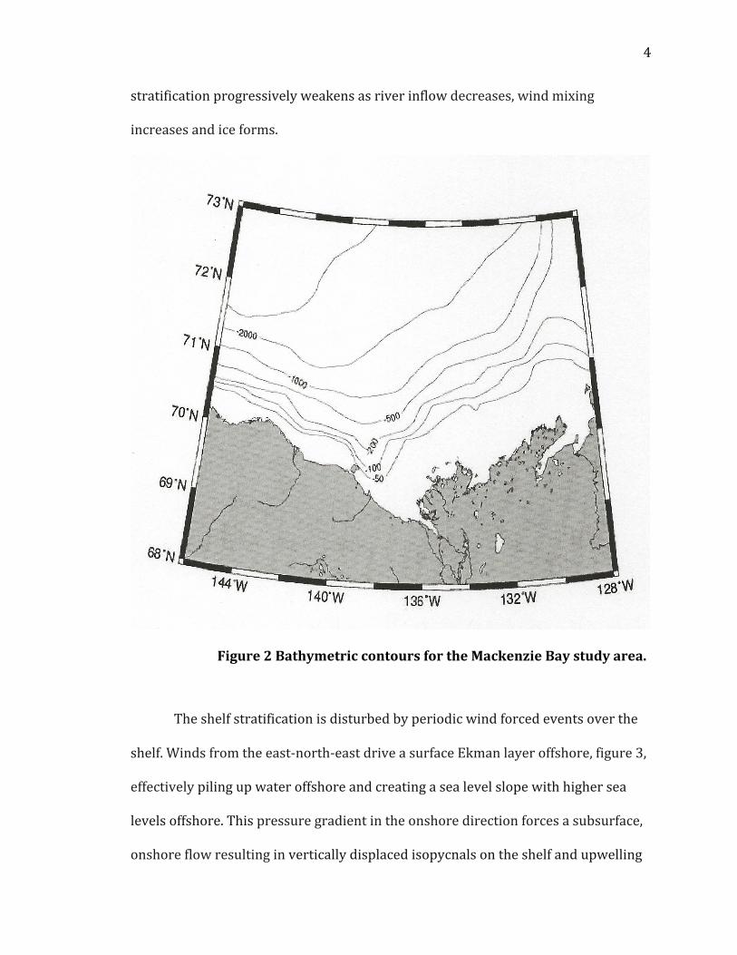
Figure 1 Map of the Arctic Ocean, the Mackenzie Bay Area is outlined in red.

3

1.1 Setting

The Mackenzie Bay is a shelf region just north of the Canadian-‐Alaskan

border and immediately adjacent to the deep Arctic Ocean; see figure 1 . This shelf

region as defined by the 100-‐m isobath is 100-‐150 km wide.

The topography consists of a uniformly sloping shelf with a mean depth of 35 m and

slope of 0.1 %. The Mackenzie Canyon intersects this relatively fiat shelf; see figure

2 for the bathymetry of this area, a deep U-‐shaped canyon with a width of 65 km and

length of 90 km. Mackenzie Canyon is wide compared to the internal deformation

radius, averaging 6 km over this region [Carmack et al., 1989]. Another prominent

feature of this shelf is the inflow of fresh water from the 3 Mackenzie River. The

Mackenzie river is the fourth largest river in the Arctic and the 11th largest in the

world. Its peak discharge occurs in the summer season when maximum volume

fluxes reach 26,000 m3/s. Its annual volume flux is approximately 380 km3

[Macdonald, 1989]. The regional surface circulation in this area is dominated by the

Beaufort Gyre, a large scale, wind-‐driven, anti-‐cyclonic current located seaward of

the shelf break. Below the surface the Beaufort Undercurrent, a subsurface eastward

flow, has been observed near the shelf break.

In the ice-‐free summer season the shelf typically exhibits a very strong

seasonal halocine with a surface layer comprised of a warm and relatively fresh

layer present to a depth of 10 m. Below the seasonal halocline the temperature

drops suddenly and the salinity increases monotonically until about 50m depth

where the temperature minimum is reached. As winter approaches, surface

4

stratification progressively weakens as river inflow decreases, wind mixing

increases and ice forms.

Figure 2 Bathymetric contours for the Mackenzie Bay study area.

The shelf stratification is disturbed by periodic wind forced events over the

shelf. Winds from the east-‐north-‐east drive a surface Ekman layer offshore, figure 3,

effectively piling up water offshore and creating a sea level slope with higher sea

levels offshore. This pressure gradient in the onshore direction forces a subsurface,

onshore flow resulting in vertically displaced isopycnals on the shelf and upwelling

5

near the coast. These upwelling events seem to be magnified around the region of

the Mackenzie canyon [Kulikov, 1998]. In the canyon isopyncal displacements of

over 600m have been observed, indicating that water has been drawn into the

canyon from a depth offshore of over 650m. This large-‐scale displacement of

isopycnals suggests that large volumes of dense and nutrient rich waters are being

mixed with relatively fresh surface water in the vicinity of the canyon.

Macdonald et al. [1987] presents hydrographic data collected in 1975, a year

with much open water. The observed new productivity based on nutrient budgets

was low compared to temperate coastal waters, but it was sufficient to supply a

significant portion of the nutrients found in the upper halocline over the entire

Arctic Ocean. In 1974, a year when the ice remained close to shore, the primary

productivity was reduced by 30%. Their observations suggest that the wind is

strongly correlated with cross shelf transport in this 5 region. From a large-‐scale

point of view, coastal upwelling events may also be a key factor in understanding

how the continental shelves of the Arctic Ocean maintain the permanent halocline

and thus insolate the overlying ice cover from the warm Atlantic layer below.

A further consequence of wind-‐forced upwelling over the Mackenzie canyon

occurs when the winds relax or rotate to a non-‐upwelling favorable direction. The

upwelled waters now over the shelf are denser than the surrounding waters and

therefore sink. In the vicinity of the submarine canyon, vertical excursions caused

by the large displacements of the isopycnals act in such a way as to force a coastal-‐

trapped wave [Brink, 1991; Mysak, 1980]. Kulikov and Carmack [1998] observed this

phenomenon by calculating the spectral phase lags of maximum coherence for four

6

current meters located to the east of the Mackenzie Canyon. They conclude that an

internal Kelvin wave is generated within Mackenzie Canyon after the cessation of

upwelling favorable winds. The observed phase speed of this wave is 0.6 m/s and its

direction is in opposition to the wind-‐driven flow field. Similar waves were

generated in the vicinity of a submarine canyon after the passage of Hurricane

Andrew over the Mississippi Canyon [Keen and Glenn, 1999].

It is clear that the dynamics observed in the Mackenzie Bay region are

extremely complicated by factors such as ice cover, changing weather and

complicated geometries associated with topography and coastline. Because of these

Figure 3 Cartoon of Ekman Surface layer transport.

7

complications, a numerical simulation of a wind forced upwelling event in the

Mackenzie Bay while paying close attention to the effects of canyon topography may

help elucidate the underlying dynamics in this region. The present state of ocean

model development allows for a fairly exact simulation of all the present dynamical

features observed in the Mackenzie Bay region.

A complex bathymetry, coastline and ambient current regime may be specified as

well as realistic winds with which to force an upwelling event, but the cost of such a

model run is the complexity associated with interpreting the results. Numerical

modeling of realistic settings requires detailed knowledge of boundary conditions,

interior horizontal and vertical viscosities as well as a large resource of computer

memory and time.

Faced with the above difficulties I have decided to simplify the setting

present in the Mackenzie Bay, while maintaining many of the relevant dynamical

scales which should affect the specific processes I am interested in modeling. Those

are, wind forced upwelling over a continental slope and submarine canyon and

internal wave generation in the vicinity of submarine canyons. Instead of

considering a very complex Arctic region, I have considered two different regimes.

These are a flat shelf and slope, and a flat shelf and slope intersected by a canyon.

The remainder of the paper of organized in sections, with the next section providing

a brief literature review on the subject of submarine canyons. Section 3 presents an

analytical model of a geostrophic adjustment over a submarine canyon. Section 4

describes the numerical model and the parameter choices made for this study.

Section 5 presents a test of the choice of boundary conditions and then the

8

simulated circulation for a shelf with a canyon and a shelf without one. Section 6

comments on how these highly idealized model simulations may provide insight on

the dynamics of wind-‐driven alongshore flow interactions with submarine canyons.

9

2 Literature Review

Submarine canyons are characteristic features of many continental margins

around the world. They are locations where flow fields are altered due to the

presence of topographic irregularities. As early as 1906 oceanographers noticed

how dense waters seem to follow bathymetric features,

" ... the currents have a tendency to follow the deepest channels of the sea bottom. Where the moving water meets a projection on the sea bottom, it is deflected towards the sides, and if there be openings the waters will follow the lines of least resistance," [Nansen, 1906). Unfortunately, physical oceanographers have not studied submarine canyons

as intensely as other coastal phenomena. The reasons for this lie in the inherent

difficulties associated with deploying instruments in areas with steeply sloping side

walls; and the fact that canyons are more heavily fished than other coastal areas due

to the high productivity found there [MacDonald et al., 1987].

A large quantity of observational evidence, mostly in the geological and

biological fields, show that canyons are places where water is exchanged between

the coastal zone and the open ocean [Noble and Butman, 1989; Shepard et al., 1979].

Coastal waters are generally confined to the continental shelf because of the

presence of fronts at the shelf edge associated with energetic currents flowing along

the isobaths which represent true physical barriers to the offshore transport of

properties [Chapman, 1986). Canyons, by disrupting the mean along-‐slope flow

pattern, seem to be capable of producing significant motions across the slope

[Aagaard and Roach, 1990). This enhanced cross-‐slope transport of properties over

canyons may be of particular importance for the renewal of coastal waters.

10

Canyons are not only significant because of the existing shelf/slope

exchanges, but also because of the vertical motions steered by their steep

topography and by the mesoscale eddies developing in their vicinity [Madron,

1994]. Hence, vertical velocity is a key variable for the dynamics of canyon

circulation. It is also a crucial parameter to study the interdisciplinary effects of the

circulation since it determines the vertical exchange between nutrient-‐rich

subsurface waters and the surface euphotic layer. The detailed description, from

hydrographic and mooring data, of the three-‐dimensional circulation in the Astoria

Canyon (U.S. West Coast) in Hickey [1997] emphasizes the role of wind forcing in the

amplification of these vertical motions in the canyon. She reports estimates of

vertical velocity as large as 50 m per day (upward) and 90 m per day (downward)

within the canyon and mean currents of 10 cm/s directed onshore at the rim of the

canyon. Significant correlation (r=0.6) was found between along-‐shelf wind and

vertical velocities. Hickey observed that as the wind builds up, the mean current,

flowing with the coast on its left, is undisturbed at the surface, but a cyclonic eddy

appears in the canyon, likely spun up by potential vorticity conservation. At the

climax of the wind, this eddy gives way to a massive onshore flow in the canyon with

the surface currents still undisturbed. As the wind relaxes, the canyon eddy forms

again and the surface currents are turned towards the coast driven by the cross-‐

shore pressure gradient. In this study, Hickey also observes an asymmetric

displacement of isopycnals over the canyon due to vertical motions induced by the

canyon wall interactions with the overlying geostrophic flows.

11

One of the earliest accounts of a persistent feature located in the vicinity of a

submarine canyon which disrupted local flows was made by Freeland and Denman,

[1982]. Their data clearly show that upwelling can take place in the absence of local

wind forcing, which led them to coin the term "topographic upwelling" as it

occurred in the head of Spur canyon, one of the branches of Juan de Fuca Canyon on

the north-‐west coast of the US. Their observations suggest that the geostrophic flow

above the canyon crosses isobaths, in the same direction as the large-‐scale flow,

thereby imposing an along-‐canyon pressure gradient. They argue that the Coriolis

force cannot balance the pressure gradient as the cross canyon velocity goes to zero

at the canyon walls. From an energetic argument they conclude that the pressure is

enough to balance the increase of potential energy as waters are upwelled from 450

m deep to the surface. Their analytical model of a non-‐linear steady flow, neglecting

the along-‐canyon Coriolis force, portrayed the first picture of how ageostrophic

pressure-‐driven flow acts in a canyon. Although very slow (typically 1 cm/s) this

kind of flow can be enough to provide a large supply of nutrients to the surface

waters.

Since that publication, other accounts of sub-‐tidal along-‐canyon flows, driven

by pressure gradients, have been reported. An example is found in Lydonia Canyon

(US East Coast) [Noble and Butman, 1989]. This particular study decomposes the

flow into empirical orthogonal functions, an analysis technique that revealed two

significant modes. An "along-‐shelf" mode, very similar to the observations described

by Freeland and Denman [1982], where along-‐shore geostrophic flow drives waters

along the shelf due to an alongshore pressure gradient. And an "exchange-‐mode"

12

characterized by an onshore flow at surface and offshore flow out of the canyon. The

dominant mode is the "along-‐shelf" in particular at low frequencies (less than 0.2

cpd) while at higher frequencies the exchange mode is dominant. These frequencies

happen to make up the bulk of the wind spectrum.

Noble and Butman conducted further analysis on the dynamics present

within Lydonia Canyon by computing force balances above the canyon and within

the canyon. They find that the flow over the shelf is primarily geostrophic, with the

pressure gradient balancing the along-‐shelf flow. Within the canyon, the geostrophic

force balance is disrupted because the cross-‐canyon currents are blocked by the

walls of the canyon. Near the rim of the canyon, turbulent Reynolds stresses, the

Coriolis force and the acceleration terms can balance the imposed pressure

gradient. The turbulent stresses arise due to the large tidal currents present in this

region. Deeper within the canyon, the Coriolis force is found to be less important,

and baroclinic adjustments begin to become an important factor in the momentum

balance.

These findings agree with those of Signorini et al. [1997] where observations

and model results show that the along-‐canyon momentum balance in Barrow

Canyon is ageostrophic, since the temporal Rossby number is of the order of 1. In

this study, the cross-‐canyon momentum balance is also analyzed, and the

researchers found that the barotropic component of the cross-‐canyon momentum

balance is geostrophic, whereas the baroclinic component is ageostrophic. For the

baroclinic component of the flow, the pressure gradient is balanced by the

acceleration and non-‐linear terms in the momentum balance as well as the Coriolis

13

force. The imbalance between the baroclinic and barotropic components of the flow

generate secondary flows with a magnitude that is between 5-‐15% of the along-‐

canyon velocities. These secondary flows, although weak; influence the structure of

the along-‐canyon flow by changing the horizontal and vertical distributions of

momentum.

Another study of interest is that of Hunkins [1988] in Baltimore Canyon. At

depths above the rim of the canyon, 100 m, a very clear cross canyon flow to the

southwest is driven by a surface pressure gradient. Below this surface layer, flow is

down-‐canyon at the head of the canyon (i.e. in the sense expected due to the surface

pressure gradient). Towards the mouth of the canyon and at depths of 600m the

flow is cyclonic, moving up-‐canyon on the northern flanks and down-‐canyon on the

southern flank. Therefore, the general pattern of flow derived from these

measurements is that of an along-‐shore flow over the canyon while within the

canyon the flow is dominantly cross-‐shore with its direction given by the pressure

gradient in geostrophic balance with the surface flow. These flows can be

responsible for steady upwelling, in the absence of local wind forcing.

Early modeling experiments showed that unstratified flows usually followed

isobaths, even at the surface. This is true of analytical and geostrophic adjustment

models by Klinck, [1989; 1988] and Chen and Allen, [1996]. Primitive equation

models with adequate stratification are able reproduce the ageostrophic flow

observed and described above. Allen [1996] reproduced the along-‐shore crossing of

isobaths of the surface flow and deeper onshore flow in the canyon in the same

direction as if it was driven by the surface pressure gradient. In the same study the

14

wind was modeled by a uniform mass sink at the coast, thereby representing the

Ekman layer without the added cost of additional layers. This simple model shows

that the onshore flow is funneled by the canyon, pumping offshore water onto the

shelf.

Han et al. [1980] found that upwelling favorable winds tended to pile water

up over the Hudson Canyon, located in the New York Bight. He utilized a finite-‐

element, steady state diagnostic model forced by local winds. Klinck [l996]

investigated the impact of flow direction and stratification on the flow in a

numerical model of pressure driven flow over smoothly varying canyon topography.

In his weakly and strongly stratified cases, flows simulating upwelling and

downwelling conditions were shown to have vastly different effects on the

processes leading to cross-‐shelf exchange. Downwelling flows tended to follow

isobaths and upwelling flows tended to push water up onto the shelf due to

baroclinic adjustments within the fluid.

15

3 Analytical Model

3.1 Problem formulation for a 2-‐layer adjustment

Klinck [1988; 1989] pioneered the development of analytical models to

explain circulation over submarine canyons. His approach was to apply a

geostrophic adjustment to a flow over a channel. With his solutions, Klinck was able

to describe a number of important features of the circulation on continental shelves

intersected by a canyon. Based on his work, simple solutions of the Navier-‐Stokes

equations can be readily derived, and provide a basis on which numerical solutions

can be judged.

The model equations are posed in "level" format [Pedlosky, 1987], which is

best thought of as a finite difference representation of the vertical gradients in the

Figure 4 Side view of the two level model. The variable for each level of the model is indicated.

16

governing primitive equations. The model setup is such that a coastal current is

driven by a surface pressure gradient. There is a submarine canyon that is situated

perpendicular to the geostrophically driven flow and the model has two levels; see

figure 4. The finite difference

approximation to the potential-‐vorticity equation permits continuous stratification

while confining the surface level to the shelf and the lower level to the canyon.

Initially the lower and upper layers are in geostrophic balance with the free-‐surface

pressure gradient. The structure of the initial flow takes the form of a sine function

varying only in the along-‐canyon canyon direction; see figure 5 .

Figure 5 The along-‐canyon structure of the initial sea surface and cross-‐canyon velocity.

17

The governing equations in terms of non-‐dimensional variables for inviscid

flow over the region above the canyon (0<x<1, where 𝑙 = !"!" , the non-‐dimensional

width of the canyon) are

𝜕𝑢!𝜕𝑡 = 𝑣! −

𝜕𝜂𝜕𝑥

(1)

𝜕𝑣!𝜕𝑡 = −𝑢! −

𝜕𝜂𝜕𝑦 (2)

𝜕𝜂𝜕𝑡 = −𝛿!

𝜕𝑢!𝜕𝑥 +

𝜕𝑣!𝜕𝑦 − 𝛿!

𝜕𝑢!𝜕𝑥 +

𝜕𝑣!𝜕𝑦 (3)

𝜕𝑢!𝜕𝑡 = 𝑣! −

𝜕𝜂𝜕𝑥 − ℇ!

𝜕𝜌!𝜕𝑥

(4)

𝜕𝑣!𝜕𝑡 = −𝑢! −

𝜕𝜂𝜕𝑦 − ℇ!

𝜕𝜌!𝜕𝑦 (5)

𝜕𝜌!𝜕𝑡 = −𝛿!

𝜕𝑢!𝜕𝑥 +

𝜕𝑣!𝜕𝑦 (6)

The parameters in (3-‐6) are the non-‐dimensional thicknesses of the levels, 𝐻! 𝐷, for

i=1,3 and the stratification parameter, 𝜀! =!!!!

∙ !!"

𝜌 , where 𝜌(𝑧) is the

temporal and spatial mean stratification.

The variables are non-‐dimensionalized as

18

𝑢∗, 𝑣∗ ~𝑈 (7)

𝑥∗,𝑦∗ ~(𝑔𝐷)!/!/𝑓 (8)

𝑡∗~ 𝑓!! (9)

𝜂∗~𝜂! = 𝑈 𝐷 𝑔 !/! (10)

𝜌∗~− 𝜂!𝑑𝑑𝑧 𝜌

(11)

The vorticity equation for each level is obtained by cross-‐differentiating the

momentum equations and substituting from the continuity equation. The resulting

equations are integrated in time to give.

𝜁! + 1𝛿!

−𝜂 + 𝜌! = 𝐶!(𝑥,𝑦) (12)

𝜁! + 1𝛿!

𝜌! = 𝐶!(𝑥,𝑦) (13)

Where 𝜆! =!!!!"− !!!

!" is the relative vorticity for level i and the integration

constants, Ci , are determined from the initial conditions. The governing equations

for the final adjusted state are obtained from the divergence of the momentum

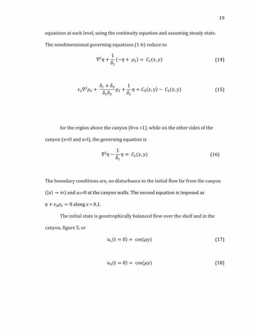
19

equations at each level, using the continuity equation and assuming steady state.

The nondimensional governing equations (1-‐6) reduce to

∇!𝜂 +1𝛿!

−𝜂 + 𝜌! = 𝐶!(𝑥,𝑦) (14)

𝜖!∇!𝜌! + 𝛿! + 𝛿!𝛿!𝛿!

𝜌! +1𝛿!𝜂 = 𝐶! 𝑥,𝑦 − 𝐶!(𝑥,𝑦) (15)

for the region above the canyon (0<x <1), while on the other sides of the

canyon (x<O and x>l), the governing equation is

∇!𝜂 −1𝛿!𝜂 = 𝐶!(𝑥,𝑦) (16)

The boundary conditions are, no disturbance to the initial flow far from the canyon

𝑥 → ∞ and u3=0 at the canyon walls. The second equation is imposed as

𝜂 + 𝜀!𝜌! = 0 along x = 0,1.

The initial state is geostrophically balanced flow over the shelf and in the

canyon, figure 5, or

𝑢! 𝑡 = 0 = cos(𝜇𝑦) (17)

𝑢! 𝑡 = 0 = cos(𝜇𝑦) (18)

20

𝜂 𝑡 = 0 = −1𝜇 sin(𝜇𝑦) (19)

𝜌! 𝑡 = 0 = 0 (20)

where 𝜇 = !!!

!"!

and Lc = 50 km, the dimensional width scale of the initial

forcing current.

The potential vorticity for the initial state is

𝐶! = 𝜇 +1𝛿!𝜇

sin 𝜇𝑦 = 𝐶! sin(𝜇𝑦) (21)

𝐶! = 𝜇 sin(𝜇𝑦) (22)

Given the trigonometric structure of the forcing, the solution to (14) and (15)

can be found in the form

𝐶! = 𝜇 +1𝛿!𝜇

sin 𝜇𝑦 = 𝐶! sin(𝜇𝑦) (23)

𝐶! = 𝜇 sin(𝜇𝑦) (24)

The x structure of the solution on either side of the canyon is obtained by

integrating

21

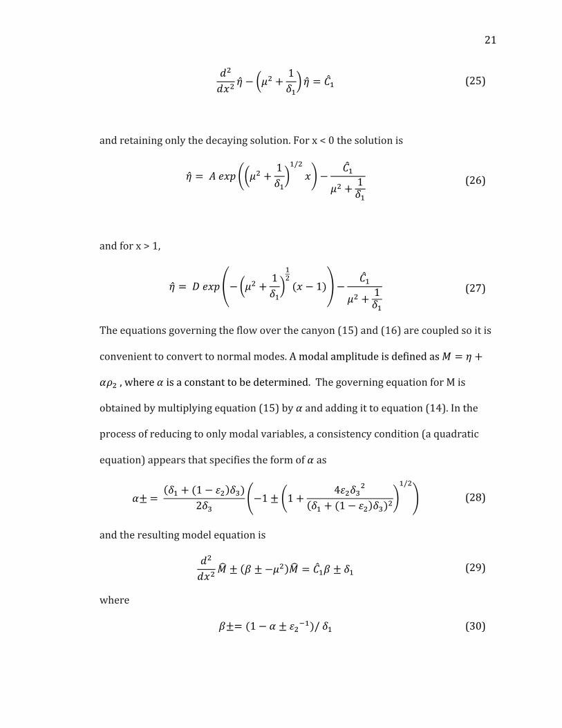
𝑑!

𝑑𝑥! 𝜂 − 𝜇! +1𝛿!

𝜂 = 𝐶! (25)

and retaining only the decaying solution. For x < 0 the solution is

𝜂 = 𝐴 𝑒𝑥𝑝 𝜇! +1𝛿!

!/!

𝑥 −𝐶!

𝜇! + 1𝛿!

(26)

and for x > 1,

𝜂 = 𝐷 𝑒𝑥𝑝 − 𝜇! +1𝛿!

!!(𝑥 − 1) −

𝐶!

𝜇! + 1𝛿!

(27)

The equations governing the flow over the canyon (15) and (16) are coupled so it is

convenient to convert to normal modes. A modal amplitude is defined as 𝑀 = 𝜂 +

𝛼𝜌! , where 𝛼 is a constant to be determined. The governing equation for M is

obtained by multiplying equation (15) by 𝛼 and adding it to equation (14). In the

process of reducing to only modal variables, a consistency condition (a quadratic

equation) appears that specifies the form of 𝛼 as

𝛼± = 𝛿! + (1− 𝜀! 𝛿!)

2𝛿!−1± 1+

4𝜀!𝛿!!

𝛿! + (1− 𝜀! 𝛿!)!

!/!

(28)

and the resulting model equation is

𝑑!

𝑑𝑥!𝑀 ± 𝛽 ±−𝜇! 𝑀 = 𝐶!𝛽 ± 𝛿! (29)

where

𝛽±= (1− 𝛼 ± 𝜀!!!)/ 𝛿! (30)

22

The surface elevation and density are recovered from the modal variables as

𝜂 =(𝛼!𝑀! − 𝛼!𝑀!)

𝛼! − 𝛼! (31)

𝜌! =𝑀! −𝑀!

𝛼! − 𝛼! (32)

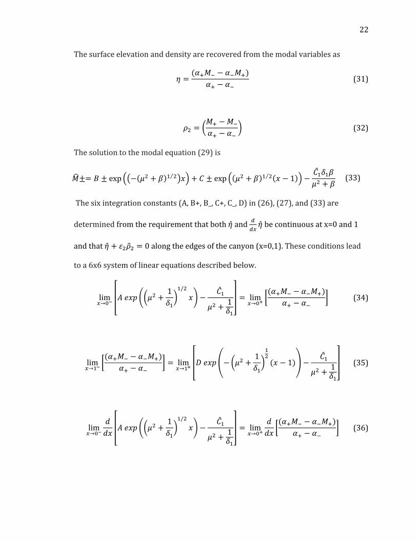
The solution.to the modal equation (29) is

𝑀±= 𝐵 ± exp − 𝜇! + 𝛽 ! ! 𝑥 + 𝐶 ± exp 𝜇! + 𝛽 ! ! 𝑥 − 1 −𝐶!𝛿!𝛽𝜇! + 𝛽

(33)

The six integration constants (A, B+, B_, C+, C_, D) in (26), (27), and (33) are

determined from the requirement that both 𝜂 and !!"𝜂 be continuous at x=0 and 1

and that 𝜂 + 𝜀!𝜌! = 0 along the edges of the canyon (x=0,1). These conditions lead

to a 6x6 system of linear equations described below.

lim!→!!

𝐴 𝑒𝑥𝑝 𝜇! +1𝛿!

!/!

𝑥 −𝐶!

𝜇! + 1𝛿!

= lim!→!!

(𝛼!𝑀! − 𝛼!𝑀!)𝛼! − 𝛼!

(34)

lim!→!!

(𝛼!𝑀! − 𝛼!𝑀!)𝛼! − 𝛼!

= lim!→!!

𝐷 𝑒𝑥𝑝 − 𝜇! +1𝛿!

!!(𝑥 − 1) −

𝐶!

𝜇! + 1𝛿!

(35)

lim!→!!

𝑑𝑑𝑥 𝐴 𝑒𝑥𝑝 𝜇! +

1𝛿!

!/!

𝑥 −𝐶!

𝜇! + 1𝛿!

= lim!→!!

𝑑𝑑𝑥

(𝛼!𝑀! − 𝛼!𝑀!)𝛼! − 𝛼!

(36)

23

lim!→!!

𝑑𝑑𝑥

(𝛼!𝑀! − 𝛼!𝑀!)𝛼! − 𝛼!

= lim!→!!

𝑑𝑑𝑥 𝐷 𝑒𝑥𝑝 − 𝜇! +

1𝛿!

!!(𝑥 − 1) −

𝐶!

𝜇! + 1𝛿!

(37)

The last two equations, (37) and (37), in the 6x6 set of linear equations are

based on the requirement of 𝜂 + 𝜀!𝜌! = 0 along the edges of the canyon (x=0,1).

This leads to the one final equation evaluated at x=O and at x=l:

(𝛼!𝑀! − 𝛼!𝑀!)𝛼! − 𝛼!

+ 𝜀!𝑀! −𝑀!

𝛼! − 𝛼!= 0 (38)

3.2 Analytical Model Results

The first two model runs presented are identical to those presented in Klinck

[1989] they are shown here to verify the numerics of the model. The third run is

highly akin to the situation present in Mackenzie Bay. In these two-‐layer simulations

the steady-‐state momentum equations are solved analytically. From the solution

four non-‐dimensional length scales emerge: μ-‐1 the y-‐structure of the initial flow

(figure 5); the external deformation radius away from the canyon, 𝛿!; and the

external and internal deformation radii over the canyon, 𝛽!!!/! and 𝛽!!!/!

respectively. Thus for parameters representing typical coastal 22 shelf systems

(depths of l00 m, density gradients of 2 kg/m3 per l00 m), coastal currents are found

of width 10-‐50 km, external radii are 200-‐400 km and internal radii are 2-‐ l0 km.

The non-‐dimensional parameters which represent the barotropic mode are O(1),

the along-‐shelf scale of the initial current is O(10-‐1), and the baroclinic scale is O(10-‐

2). From this non-‐dimensional order of magnitude analysis, we can conclude that the

24

influence of a coastal canyons on a typical shelf will decay with the width scale of the

initial current. Over the canyon, the baroclinic mode will decay away from the

canyon with the width scale of the internal radius of deformation and the barotropic

mode will decay with the scale of the forcing current.

For a simulation of a wide canyon, 200 km; figure 6, the cross-‐canyon flow

above the canyon is slowest at the edges of the canyon, and the influence of the

Figure 6 The adjusted, steady state across canyon sea surface height , level 2 density anomaly, level 1 velocities, and layer 2 velocities for a canyon that is 10 km wide.

25

canyon decays with the scale of the initial current, 50 km. The along canyon flow

both above and within the canyon seem to be strongly affected by the pressure

gradients. Displacements of the sea surface; figure 6, reveal a bulge of fluid above

the canyon reaching a maximum of about 0.75 cm above the canyon walls. This

pressure gradient drives flow vertically so as to oppose the surface elevations

initially prescribed. The effect of these vertical excursions of the fluid within the

canyon is to stretch and shrink vortex tubes, thereby creating regions of cyclonic

Figure 7 The adjusted, steady state across canyon sea surface height, level 2 density anomaly, level 1 velocities, and layer 2 velocities for a canyon that is 200 km wide.

26

and anti-‐cyclonic vorticity. In this particular model run, lower layer

maximum isopycnal displacements are about 10 m. These small displacements of

the isopycnals in comparison to the findings of Freeland and Denman [1982] or of

Kulikov [1997] are a direct result of the weak forcing (10 cm/s) and weak

stratification (!"!" = -‐0.02 kg/m3 ) in this run.

Figure 8 The adjusted, steady state across canyon sea surface height, level 2 density anomaly, level 1 velocities, and layer 2 velocities for a canyon that is 40 km wide.

27

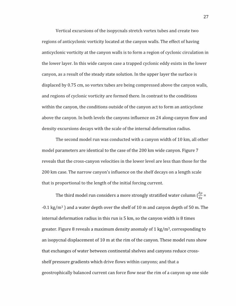
Vertical excursions of the isopycnals stretch vortex tubes and create two

regions of anticyclonic vorticity located at the canyon walls. The effect of having

anticyclonic vorticity at the canyon walls is to form a region of cyclonic circulation in

the lower layer. In this wide canyon case a trapped cyclonic eddy exists in the lower

canyon, as a result of the steady state solution. In the upper layer the surface is

displaced by 0.75 cm, so vortex tubes are being compressed above the canyon walls,

and regions of cyclonic vorticity are formed there. In contrast to the conditions

within the canyon, the conditions outside of the canyon act to form an anticyclone

above the canyon. In both levels the canyons influence on 24 along-‐canyon flow and

density excursions decays with the scale of the internal deformation radius.

The second model run was conducted with a canyon width of 10 km, all other

model parameters are identical to the case of the 200 km wide canyon. Figure 7

reveals that the cross-‐canyon velocities in the lower level are less than those for the

200 km case. The narrow canyon's influence on the shelf decays on a length scale

that is proportional to the length of the initial forcing current.

The third model run considers a more strongly stratified water column (!"!" =

-‐0.1 kg/m3 ) and a water depth over the shelf of 10 m and canyon depth of 50 m. The

internal deformation radius in this run is 5 km, so the canyon width is 8 times

greater. Figure 8 reveals a maximum density anomaly of 1 kg/m3, corresponding to

an isopycnal displacement of 10 m at the rim of the canyon. These model runs show

that exchanges of water between continental shelves and canyons reduce cross-‐

shelf pressure gradients which drive flows within canyons; and that a

geostrophically balanced current can force flow near the rim of a canyon up one side

28

and down the other. The magnitude of the predicted flow in the canyon decreases as

the canyon narrows. Increasing stratification in this analytical simulation leads to

increased along canyon flows within the canyon but does not change the flow

characteristics above the canyon rim. The effect of compressing and stretching of

Taylor columns below the canyon rim leads to the formation of a trapped cyclonic

eddy. Above the canyon rim, a trapped anticyclonic eddy is formed.

29

4 Problem Formulation for Numerical Simulations

The underlying physics present in the analytical model above represent steady-‐

state, inviscid and linear dynamics. As earlier observations have shown, not all

submarine canyons behave in a linear manner and the assumption of frictionless

flow certainly can not help to clarify the effect of the winds. The underlying

assumption of geostrophy may also be incorrect as the baroclinic adjustments

leading to secondary flows are certainly not geostrophic. Because of these

complications, a numerical simulation which solves the full set of Navier-‐Stokes

equations for a wind-‐forced upwelling event in the Mackenzie Bay may help

elucidate the underlying dynamics in this region.

Numerical simulations presented in this paper were made with version 3.0

of the S-‐Coordinate Rutgers University Model (SCRUM). SCRUM utilizes the

Boussinesq approximation in which density variations are assumed to be small in

comparison to a mean density except when gravitational forces are essential.

SCRUM also assumes that the dominant force balance in the vertical momentum

equation is between the vertical pressure gradient and the gravitational force, the

hydrostatic assumption. SCRUM solves the shallow water forced equations of

motion over a terrain-‐following, stretched sigma coordinate system with a free

surface [Hedstrom, 1997]. The model is designed for circulation in an environment

with strong changes in bottom topography, weak friction and non-‐linear dynamics.

The grid discretization used in SCRUM is a centered, second-‐order finite

difference approximation in the horizontal and vertical with the staggered Arakawa

30

"C" grid arrangement of variables. SCRUM utilizes a fractional step method to couple

barotropic and baroclinic modes in the split-‐explicit time stepping procedure. The

depth-‐integrated equations of motion are solved on a short time step due to the

presence of the free surface. The integrated values of the barotropic mode are then

substituted into the full 3-‐D equations of motion which are integrated on a longer

timestep [Hedstrom, 1997]. For the barotropic mode the model is time stepped from

time n to n + 1 via a leapfrog, centered in time and space method. This method is

accurate to O(∆𝑡!) but it is unconditionally unstable with respect to diffusion

processes. In order to counteract this a trapezoidal correction is applied every time

step. This combination of a leapfrog predictor and a trapezoidal corrector time

stepping is stable with respect to diffusion and strongly damping in respect to

errors arising out of the computational mode. The only disadvantage to this

combination of a leapfrog/trapezoidal predictor/corrector is that it requires twice

as much computation time as compared to the pure leapfrog method. The full 3-‐D

fields are time-‐stepped via a third-‐order Adams-‐Bashforth method [Haidvogel and

Beckman, 1999]. Time stepping limitations arise due to instabilities which can grow

unbounded; the constraint is usually referred to the CFL condition. The model runs

presented herein use a 50 second time step for the barotropic mode and a 250

second time step for the baroclinic mode; the CFL condition specifies that a

minimum time step of 90 seconds is required for numerical stability.

The simulated coastal domain is 100 km long in the cross-‐shore direction

and 300 km long in the alongshore direction. The domain has a single, straight,

coastal wall on its western boundary. In order to make comparisons between the

31

analytical model and the numerical model more straightforard, at the coast a free

slip, or no stress, condition is applied. The no stress condition neglects frictional

effects of flow normal to the coastline. To the north and south I have specified a

periodic boundary which allows particles with all of their dynamical properties to

propagate out of the boundary and back in on the other side. A simple

representation of the periodic boundary condition is a rotating, circular flume tank.

Geometrically, the periodic boundary conditions resemble an annulus.

For the offshore boundary along the eastern edge I have specified an Orlanski

type radiation boundary condition. This boundary condition prevents waves or

tracers from being reflected back into the domain once they reach this outer

boundary. This is achieved by evaluating the phase speed at which a tracer, the free

surface or the cross-‐ shelf velocity is approaching the boundary at each time step.

The computed phase speed is then used in a Sommerfield type radiation condition

at the boundary [Chapman, 1985]. I have also utilized the Large et al. [1994]

turbulence closure scheme in these model runs.

The model domain is 10 m deep at the coast and 50m deep offshore, the

canyon is 40km wide and 50km long. These parameter choices were chosen to

closely simulate the bathymetry of the Mackenzie Canyon and Bay. To the East of the

Mackenzie Canyon, the direction of interest for the propagation of coastally trapped

waves, the shelf depth is approximately 50 m deep out to 100 km offshore where

the shelf break and depths of 2000 m are encountered [Kulikov et al., 1998]. The

maximum slope anywhere in the domain is about 0.1 %; see figure 9 and table 2 for

a complete description of the geometric length scales used in these simulations.

32

Over this domain I have specified a grid that is 2 km by 2 km in the horizontal and

contains 20 vertical levels in the stretched sigma coordinate system. I have

incorporated bottom friction by specifying that the flow must obey a quadratic

decay law, which forces the velocity to reach zero at the sea floor. The bottom drag

coefficient used here is_3 x 10-‐3. These model runs simulate idealized conditions

present off of the Mackenzie Shelf in the summer, stratified season; see figure 10.

The model is started from rest and is forced by a 3.5 m/s wind from the

south, upwelling favorable. This corresponds to a wind stress of 0.03 N/m2

according to the formulae of Wu [1980]. The winds are ramped up over a period of 2

days with a sinusoidal function; this is done to minimize the number of initial

transients, which are not removed from the domain due to the periodic boundary

conditions. After model day two, the winds are uniform and constant up to day

seven. At day seven the winds are shut off abruptly in an effort to allow upwelled

Figure 9 Bathymetry of the two cases.

33

isopycnals to slump into the interior, thereby becoming the forcing mechanism for

internal waves [Beletsky et. al., 1997; Keen and Allen, 2000].

Model parameters are given in table 1, the non-‐dimensional numbers are

computed using the methods as presented in Munchow and Garvine [1993]. The

flows that are presented in this paper are low Rossby number flows, meaning that

they are weakly nonlinear.

They have a Burger number of O(10-‐1) indicating that the flow may be modified

substantially by the relative vorticity produced by variations in topography. And

these flows are also of low Froude number, indicating that particle speeds are much

Figure 10 Cross-‐shelf structure of the initial density profile used in the model runs, values given are sigma-‐t with units of kg/m3.

34

smaller than internal wave speeds, and thus implies a subcritical flow. One can infer

from the small Rossby number and the Froude number less than 1 that both

stratification and rotation are dynamically important.

35

5 Numerical Simulations

5.1 Boundary Condition Verification

In order to verify that the periodic boundary conditions specified in these

model runs do not significantly alter coastally trapped waves, I have constructed a

test of these boundary conditions. A fiat bottom, barotropic kelvin wave has an

analytical solution which is most easily applied as an initial condition; see Gill

[1982] for a complete review of Kelvin wave dynamics. Assuming only linear,

inviscid dynamics, this type of wave should propagate uniformly along a coastal

wall. In the case of the periodic boundary condition, the effectiveness of this type of

boundary condition may be evaluated. In figure 7, contours of sea surface height for

time zero of the analytical solution for the fiat bottom kelvin wave are shown. In this

model run a kelvin wave with a wavelength of 100 km is prescribed. The model has

a depth of l00 m so this wave has an analytical phase speed corresponding to 31.3

m/s, and a period of 53.23 minutes. Spectral analysis computed by utilizing the Fast

Fourier Transform of the mean removed sea surface height at stations 1 through 4,

see figure 12, reveals a spectral peak at 3.12 x 10-‐4 Hz, corresponding to a period of

53.4 minutes. This difference of periods between the analytical solution and the

computed numerical approximation corresponds to an error of 0.3%. Taking into

account the fact that these waves had to be discretized onto a 2 km grid, this is well

within the levels of error associated with stable numerics. A second spectral peak at

exactly twice the frequency of the first peak can also be seen in the periodigram for

sea level. This spectral peak is 5 orders of magnitude smaller that the first peak and

36

probably corresponds the first harmonic arising due to some non-‐linear interactions

within the model. Error bars show that this second peak is hardly discernable as

compared to the background noise.

Figure 11 Contours of sea surface height and station locations for the boundary condition verification runs. Solid lines represent a piling up of the free surface and dashed lines represent a depression of the free surface.

In order to assess the propagation of these waves on a numerical grid an

analysis technique developed by Kundu and Allen [1976] termed the "lagged"

correlation function is used. This technique computes the cross correlation for

various time lags in sea level, currents or isopycnal displacements between two

stations. A plot of time lag for maximum correlation versus the alongshore distance

of separation between stations can then yield an estimate for the phase speed of a

propagating feature. In figure 13, maximum correlation versus alongshore

separation reveals that the phase speed of the propagating feature is 30.6 m/s, an

37

error of 2.2%. Again the error associated with the phase speed of barotropic kelvin

waves on this numerical grid is neglible as compared to the errors, which might be

Figure 12 A time series of sea surface height and its associated power spectra for station 1.

expected from an improper grid resolution. We therefore conclude that periodic

boundary conditions do not significantly alter the propagation of these waves and

that the horizontal grid resolution of 2 km is sufficient.

5.2 Shelf without canyon

In the model run without a canyon the northerly alongshore winds create an Ekman

type surface flow in the offshore direction; see figure 3 for a schematic of Ekman

38

transport. The net mass transport of the surface layer offshore leads to a pressure

gradient directed onshore. This can be seen in the free surface elevation, which is

uniformly increasing in the offshore direction; see figure 14. An onshore subsurface

flow is forced in response to this pressure gradient. Isopycnal displacements are

observed to take place within a day after the onset of the winds and a long shore

current flowing northward develops soon afterwards. This alongshore current is a

result of the geostrophic balance between the Coriolis force directed offshore and

the pressure gradient directed onshore. The upwelling elevates isopycnals at the

coast uniformly in the along shore direction. Over the shelf and slope there is no

along-‐shore variability in the velocity field; see figure 14. Upon cessation of the wind

the upwelling continues for a short period of time but the long shore flows seem to

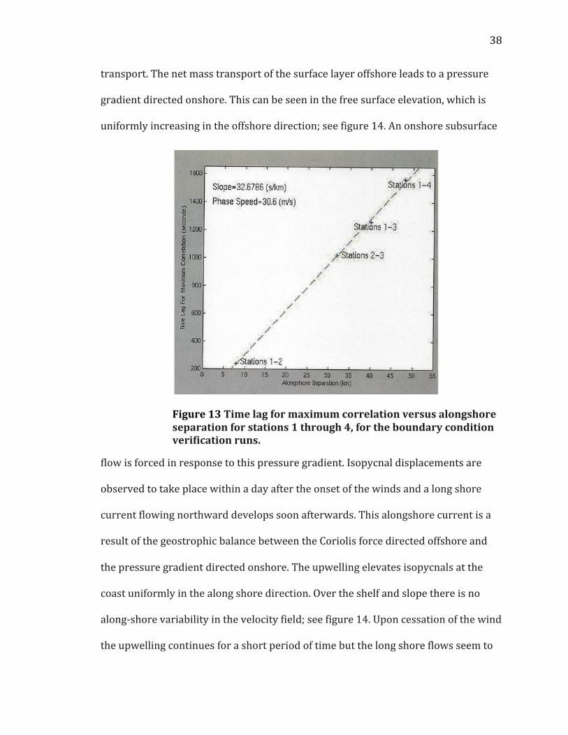
Figure 13 Time lag for maximum correlation versus alongshore separation for stations 1 through 4, for the boundary condition verification runs.

39

dissipate rather quickly, due to the drop in the sea surface and subsequent decrease

in the cross-‐shore pressure gradient; see figure 15.

Figure 14 Contours of the free surface elevation at model day 5.25, values have been averaged over one inertial period.

There is no isolated pooling of dense water on the shelf during the upwelling or

Figure 15 Time series of sea surface height at station 3, located on the shelf break, for the run without a canyon. Station data is written to a file at every baroclinic step of the model, 250 seconds.

40

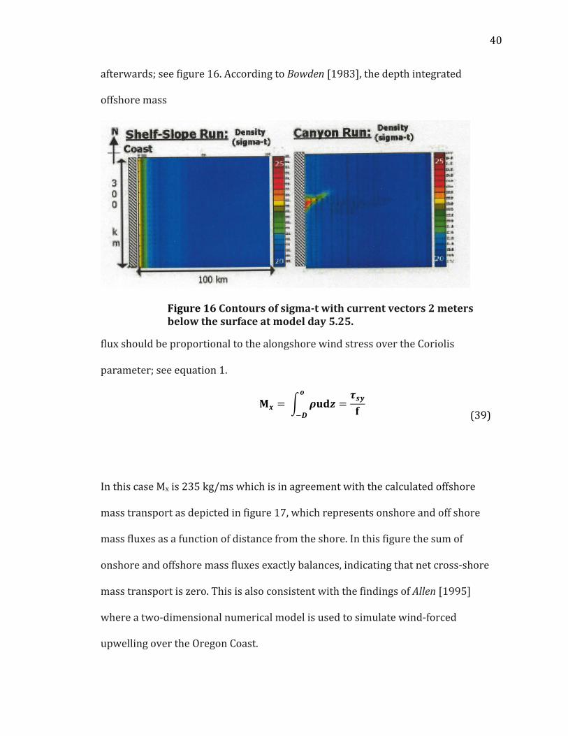
afterwards; see figure 16. According to Bowden [1983], the depth integrated

offshore mass

Figure 16 Contours of sigma-‐t with current vectors 2 meters below the surface at model day 5.25.

flux should be proportional to the alongshore wind stress over the Coriolis

parameter; see equation 1.

𝐌𝒙 = 𝝆𝐮𝐝𝒛 =𝝉𝒔𝒚𝐟

𝒐

!𝑫

(39)

In this case Mx is 235 kg/ms which is in agreement with the calculated offshore

mass transport as depicted in figure 17, which represents onshore and off shore

mass fluxes as a function of distance from the shore. In this figure the sum of

onshore and offshore mass fluxes exactly balances, indicating that net cross-‐shore

mass transport is zero. This is also consistent with the findings of Allen [1995]

where a two-‐dimensional numerical model is used to simulate wind-‐forced

upwelling over the Oregon Coast.

41

Figure 17 Across-‐shore mass flux as a function of distance from the coast for the run with no canyon. Positive and negative values represent offshore and onshore mass fluxes respectively. The dashed line represents the sum of on-‐ and off-‐shore mass fluxes.

5.3 Shelf With Canyon

For the model run with a shelf and a canyon a very different dynamical

picture evolves. The Ekman type offshore flow in the surface layer develops in much

the same way as the run without the canyon, but the onshore pressure gradient

seems to be affected by the presence of the canyon. Figure 14 reveals a bulge in the

free surface over the canyon and figure 16 shows an isolated pooling of dense water

on the shelf at the head of the canyon. Along shore surface velocities reveal an anti-‐

cyclonic turning of the flow field over the canyon. As the canyon width is

approximately ten times the internal deformation radius, table 1, I expect that the

canyon should exhibit some bathymetric steering to the flow field due to the

42

tendency for a fluid column to conserve its potential vorticity. This is very nearly the

case for the velocity field at 20 meters (not shown); as there is a strong turning

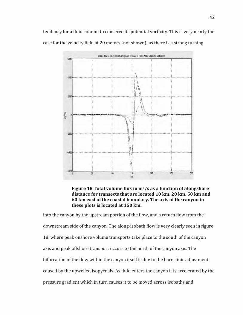
Figure 18 Total volume flux in m3/s as a function of alongshore distance for transects that are located 10 km, 20 km, 50 km and 60 km east of the coastal boundary. The axis of the canyon in these plots is located at 150 km.

into the canyon by the upstream portion of the flow, and a return flow from the

downstream side of the canyon. The along-‐isobath flow is very clearly seen in figure

18, where peak onshore volume transports take place to the south of the canyon

axis and peak offshore transport occurs to the north of the canyon axis. The

bifurcation of the flow within the canyon itself is due to the baroclinic adjustment

caused by the upwelled isopycnals. As fluid enters the canyon it is accelerated by the

pressure gradient which in turn causes it to be moved across isobaths and

43

upcanyon. The displacements of the isopycnals causes the baroclinic component of

the pressure gradient to be in the same direction as the barotropic component, and

fluid parcels are transported onto the shelf, out of the canyon. Within the canyon,

the magnitude of the return flow does not match the magnitude of the upcanyon

flow and a net displacement of water is upcanyon. This pattern of upwelled water in

the canyon agrees qualitatively with the weakly stratified upwelling case in Klinck

[1996].

As figure 18 indicates, the zero crossings of the onshore and offshore volume

fluxes are displaced towards the north as one moves onshore. It should also be

noted that onshore volume fluxes decrease substantially as one approaches the

coastal boundary and that away from the canyon the net cross shore volume flux is

zero. Of particular significance is the fact that the upstream influence of the canyon

decays with a length associated with the radius of the canyon. Where as the

downstream influence of the canyon decays with a larger length scale than that

associated with the canyon radius. This signifies that the advection of fluid taking

place due to the wind forcing is causing the effects of the canyon to be felt more

strongly in the direction that is opposite to that expected from the direction of

coastal wave propagation, i.e. with the coast on the right. Haidvogel and Brink

[1986] observed that mean currents can be generated in the vicinity of submarine

canyons with a time oscillating wind field. These mean currents are driven by the

effect of topographic form stress, their direction is in the sense of coastal wave

propagation. Due to the effect of the constant wind field I do not observe this

mechanism of topographic form stress taking place.

44

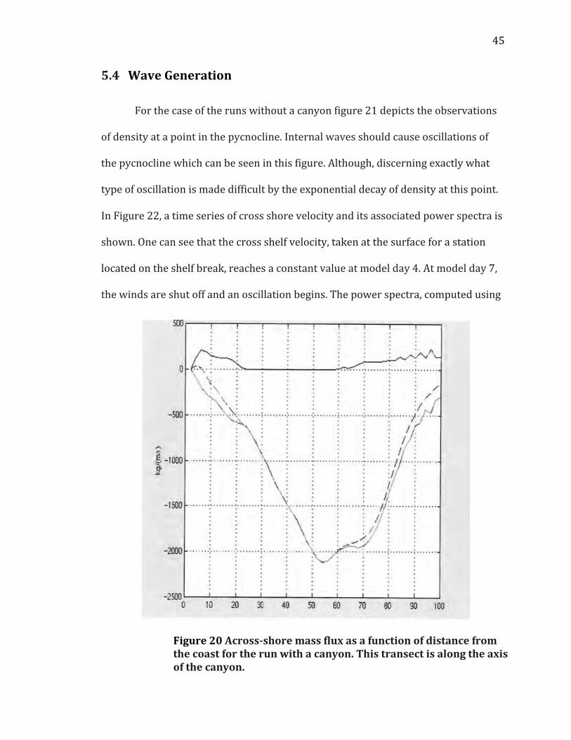
Another interesting aspect is that of the vertical velocities within and above

the canyon see figure 19 . At the mouth of the canyon I observe a vertical jet of water

directly above the central axis of the canyon. This jet is displaced northward by the

overlying flow and there seems to be a resultant down welling on the downstream

side of the canyon. The pattern of upwelling on the upstream side of the axis of the

canyon and downwelling on the downstream side of the axis is also very clearly

seen in the along-‐shore isopycnal contours. Figure 20 reveals that along the axis of

the canyon net onshore mass transport is nearly 5 times the offshore Ekman surface

transport, as calculated by equation 39.

Figure 19 Vertical velocities 1 meter above the shelf during model day 5.25. the canyon axis is located in the center. Note regions of strong up and down canyon flows. Units for the color contour are in cm/day.

45

5.4 Wave Generation

For the case of the runs without a canyon figure 21 depicts the observations

of density at a point in the pycnocline. Internal waves should cause oscillations of

the pycnocline which can be seen in this figure. Although, discerning exactly what

type of oscillation is made difficult by the exponential decay of density at this point.

In Figure 22, a time series of cross shore velocity and its associated power spectra is

shown. One can see that the cross shelf velocity, taken at the surface for a station

located on the shelf break, reaches a constant value at model day 4. At model day 7,

the winds are shut off and an oscillation begins. The power spectra, computed using

Figure 20 Across-‐shore mass flux as a function of distance from the coast for the run with a canyon. This transect is along the axis of the canyon.

46

a mean removed FFT with the record beginning at day 7, for this oscillation reveals

that the dominant frequency of this oscillation is 2. 2e-‐5 Hz. This wave form has a

period of 12.63 hours, a near-‐inertial oscillation, and it is generated at the very

moment that the-‐winds cease.

Figure 21 A density profile and a time series of density at sigma level 6 (pycnocline depth) for the run without a canyon. Station 3 is located at the shelf break.

For the canyon case, figure 23 depicts density fluctuations at stations located on the

shelf break. Again, interpretation of these fluctuations is complicated due to their

exponentially decaying nature. In figure 24, the time series of velocity for all stations

on the shelf is shown, it reveals that a wave of the same frequency as the run

without a canyon is being generated. I do not see any modification of the dominant

frequency of this wave form as I have also looked at along shore velocity, velocities

47

at mid-‐depth and bottom velocities. For the case of a canyon and a shelf without a

canyon, the same dynamical picture emerges: an inertial wave is being generated in

response to a sudden wind relaxation event.

Figure 22 Cross shore velocity at the surface for a station located on the shelf break and the associated power spectra of the time series beginning at model day 7.

These plots of velocity are easier to believe than the density time series presented

earlier. First, the velocity record does not contain the exponential decay apparent in

the density time series. And second, the velocity record begins to oscillate almost

instantaneously after the winds are shut off. The barotropic wave phase speed is 22

m/s; therefore the fastest waves circle the domain in about 4 hours. This wave form

48

that I observe in these time series plots of velocity is therefore propagating around

the domain, unmodified by the canyon topography.

Figure 23 Density Fluctuations for the stations located on the shelf break, stations 3-‐ 13 are located to the south of the canyon and stations 18 and 23 are located to the north.

49

Figure 24 Time series of cross shelf velocities at the surface for the run with a canyon.

50

6 Conclusion

The model runs that I have completed thus far show that wind forcing creates a

very different result when it occurs over a shelf with a canyon versus a shelf alone.

In both cases the winds create an Ekman type offshore flow. This offshore

displacement of the surface layer leads to a baroclinic pressure gradient directed

onshore. This pressure gradient can be seen in the free surface elevations in both

cases. A major difference in the free surface elevations is that the canyon run

influences the free surface in such a way as to create a bulge over the axis of the

canyon, whereas the shelf run creates a uniformly increasing pressure gradient

directed on shore. The shelf-‐only model run does not contain any longshore

variability in the velocity field or in the isopycnal displacements. The model run

with canyon topography does contain longshore variability as well as offshore

variability in the velocity fields. In terms of wave generation, I do not observe the

phenomena of internal Kelvin waves being generated after the cessation of

upwelling favorable winds. I do see similiar inertial responses to shutting off the

winds in model runs both, with and without canyons. Overall I have observed that

canyons act as a conduit for vertical motions during upwelling events. The surface

isopycnal outcroppings also show that a canyon tends to localize the effects of

upwelling to the coastline located shoreward of the canyon axis. Also the-‐presence

of a submarine canyon greatly enhances the mixing between shelf and offshore

waters.

51

My runs thus far do not simulate the internal waves that have been observed

in the Beaufort Sea and that is be due to several factors. First, a very weak forcing is

applied over the model domain. Current magnitudes of approximately 50 cm/s are

generated and the associated inertial radia of these flows is very small. This tends to

decrease the effects of inertial forces due the much larger effects of the particle

phase speeds within the flow. Second, my boundary conditions, which are

appropriate for the simulation of coastally trapped waves, may be inappropriate in

their ability to adequately represent exchanges of momentum at the offshore

boundary. My model domain essential reproduces a shelf of infinitely many

submarine canyons, each separated by 300 km. Although, the analytical model of

Klinck [1989] suggests that the effects of a canyon should decay with a length scale

shorter than even half this distance, I suspect that the localized exchange of fluid

within the submarine canyon is affecting processes on the shelf located hundreds of

kilometers away. Even though my domain is large enough to contain processes

which are taking place on the length scale associated with the internal deformation

radius, it does not adequately contain processes which might take place with length

scales associated with the external deformation radius i.e. barotropic kelvin waves.

The inability of these simulations to allow motions of this large scale may greatly

inhibit important dynamical processes, which are essential for the excitation of

internal waves.

In conclusion, it has been demonstrated that highly idealized numerical and

analytical simulations of flows over submarine canyons reveal many important

dynamical processes, which have been observed in the field. The limitations of these

52

models lies in their simplifications of bathymetry and their inability to accurately

reproduce flows along open boundaries: The issues associated with limiting

boundary conditions are at the forefront of computational and numerical ocean

simulation science. In the future, faster computers with greater allocations of

memory may be able to more accurately reproduce observations collected in and

around submarine canyons.

53

REFERENCES

Aagaard, K., and E.C. Carmack, The Role of Sea Ice and Other Fresh Water in the

Arctic Circulation, Journal of Geophysical Research, 94 (ClO), 14,485-‐14,498, 1989.

Aagaard, K., and E.C. Carmack, The Arctic Ocean and Climate: A Perspective, in The

Polar Oceans and Their Role in Shaping the Global Environment, Geophys . Monogr. Ser., edited by e.a. J. Johannessen, pp. 4-‐20, AGU, Washington, D.C., 1994.

Aagaard, K., L.K. Coachman, and E.C. Carmack, On the Halocline of the Arctic Ocean,

Deep-‐Sea Research, 28A (6), 529-‐545, 1981. Aagaard, K., and AT. Roach, Arctic Ocean-‐Shelf Exchange: Measurements in Barrow

Canyon, Journal of Geophysical Research, 95 (ClO), 18,163-‐18,175, 1990. Allen, S.E., Topographicall generated, subinertial flows within a finite length canyon,

Journal of Physical Oceanography, 25, 1608-‐1632, 1996. Beletsky, D., W.P. O'Conner, D.J. Schwab, and D.E. Dietrich, Numerical Simulation of

Internal Kelvin Waves and Coastal Upwelling Fronts, Journal of Physical Oceanography, 27, 1197-‐1215, 1997.

Brink, K.H., Coastal-‐Trapped Waves and Wind Driven Currents Over the Continental

Shelf, Ann. Rev. Fluid Mech. (23), 389-‐412, 1991. Carmack, E.C., R.W. Macdonald, and J.E. Papadakis, Water Mass Structure and

Boundaries in the Mackenzie Shelf Estuary, Journal of Geophysical Research, 94 (Cl2), 18,043-‐18,055, 1989.

Chapman, D.C., Numerical Treatment of Cross-‐Shelf Open Boundaries in a Barotropic

Coastal Ocean Model, Journal of Physical Oceanography, 15, 1060-‐1075, 1985. Chapman, D.C., A Simple Model of the Formation and Maintenance of the Shelf/Slope

Front in the Middle Atlantic Bight, Journal of Physical Oceanography, 16, 1273-‐ 1279, 1986.

Chen, X., and S.E. Allen, The influence of canyons on shelf currents: a theoretical

study, Journal of Geophysical Research, 101 (C8), 18,043-‐18,059, 1996. Freeland, H.J., and K.L. Denman, A Topographically controlled upwelling center off

southern Vancouver Island, Journal of Marine Research, 40 (4), 1069-‐1093, 1982.

54

Haidvogel, D.B., and K.H. Brink, Mean currents driven by topographic drag over the continental shelf and slope, Journal of Physical Oceanography, 16 (12), 2159-‐2171, 1986.

Haidvoigel, D.B., and A. Beckman, Numerical Ocean Circulation Modeling, 320 pp.,

Imperial College Press, London, 1999. Han, G., D.V. Hansen, and J.A. Galt, Steady-‐State diagnostic model of the New York

Bight, Journal of Physical Oceanography, 10, 1998-‐2020, 1980. Hedstrom, ;K.S., User's Manual For an S-‐Coordinate Primitive Equation Ocean

Circulation Model, Institute of Marine and Coastal Sciences, Rutgers University, New Brunswick, 1997.

Hickey, B.M., The response of a steep sided, narrow canyon to time-‐variable wind

forcing, Journal of Physical Oceanography, 27, 697-‐726, 1997. Hunkins, K., Mean and tidal currents in Baltimore Canyon, Journal of Geophysical

Research, 93 (C6), 6917-‐6929, 1988. Keen, T.R., and S.E. Allen, The generation of internal waves on the continental shelf

by Hurricane Andrew, Journal of Geophysical Research, 105(Cl1), 26,203-‐26,224, 2000.

Keen, TR., and S.M. Glenn, Shallow water currents during Hurricane Andrew, Journal

of Geophysical Research, 104 (ClO), 23,445-‐23,458, 1999. Klinck, J., Geostrophic adjustment over submarine canyons, Journal of Geophysical

Research, 94 (C5), 6133-‐6144, 1989. Klinck, J.M., The influence of a narrow transverse canyon on initially geostrophic

flow, Journal of Geophysical Research, 93 (Cl), 509-‐515, 1988. Klinck, J.M., Circulation near submarine canyons: A modeling study, Journal of

Geophysical Research, 101(Cl), 1211-‐1223, 1996. Kulikov, E.A., E.C. Carmack and R.W. Macdonald, Flow Variability at the continental

shelf break of the Mackenzie Shelf in the Beaufort Sea, Journal of Geophysical Research, 103 (C6), 12,725-‐12,741, 1998.

Large, W.G., J.C. Mc Williams, and S.C. Doney, Oceanic vertical mixing: a review and a

model with a nonlocal boundary layer parameterization, Rev. Geophysics (32), 363-‐403, 1994.

55

Macdonald, R.W., and C. S. Wong, The Distribution of Nutrients in the Southeastern Beaufort Sea: Implications for Water Circulation and Primary Production, Journal of Geophysical Research, 92 (C3), 2939-‐2952, 1987.

Macdonald, R.W., E.C. Carmack, F.A. McLaughlin, K. Iseki, D.M. Macdonald and M.C.

O'brien, Composition and Modification of Water Masses in the Mackenzie Shelf Estuary, Journal of Geophysical Research, 94 (C12), 18,057-‐18,070, 1989.

Madron, X.D.D., Hydrography and nepheloid structures in the Grand-‐Rhone canyon,

Continental Shelf Research, 14 (5), 457-‐477, 1994. Munchow, A., and R.W. Garvine, Dynamical properties of a buoyancy-‐driven coastal

current, Journal of Geophysical Research, 98(Cl1), 20,063-‐20,077, 1993. Mysak, L.A., Topographically Traped Waves, Ann. Rev. Fluid Mech., 12, 45-‐76, 1980. Nansen, F., Northern waters: Captian Roald Amundsen's oceanographic

observations in the Arctic Seas in 1901, Ekr. Nor. Vidensk. Akad. Kl. 1 Mat. Naturvidensk., 3, 145, 1906.

Noble, M., and B. Butman, The structure of subtidal currents within and around

Lydonia Canyon: evidence for enhanced cross-‐shelf fluctuations over the mouth of the canyon, Journal of Geophysical Research, 94 (C6), 8091-‐8110, 1989.

Pedlosky, J., Geophysical Fluid Dynamics, 710 pp., Springer-‐Verlag Inc., New York,

1987. Shepard, F.P., N.F. Marshall, P.A. Mcloughlin, and G.G. Sullivan, Currents in Submarine

Canyons and other Seavalleys, 173 pp., The American Association of Petroleum Geologists, Tulsa, Oklahoma, USA, 1979.

Signorini, S.R., A. Munchow, and D. Haidvogel, Flow dynamics of a wide Arctic

Canyon, Journal of Geophysical Research, 102 (C8), 18,661-‐18680, 1997. Wu, J., Wind Stress Coefficients over the sea surface near neutral conditions, Journal

of Physical Oceanography, JO, 727-‐740, 1980.

56

Table 1: Model Parameters

Name: Equation Shallow (H=10m):

Deep (H=50m):

Barotropic Wave Phase Speed

𝑐 = 𝑔𝐻 9.9 m s-‐1 22.1 m s-‐1

Stability Frequency 𝑁 =

𝑔𝜌!∙𝛿𝜌𝛿𝑧

0.06 s-‐1 0,026 s-‐1

Internal Wave Phase Speed 𝑐! = 𝑁𝐻 0.58 m s-‐1 1.3 m s-‐1

Coriolis Parameter 𝑓= 2Ω sin(𝜃)

1.37x10-‐4 s-‐1 1.37x10-‐4 s-‐1

Internal Deformation Radius 𝜆! =𝑐!𝑓

4.2 km 9.4 km

External Deformation Radius 𝜆! =𝑐𝑓

72 km 162 km

Inertial Radius 𝐿! =𝑈𝑓

400 m 160 m

Burger Number 𝑆 =

𝜆!𝐿

!

0.1 0.4

Rossby Number 𝑅! =𝑈𝑓𝐿

0.09 0.09

Froude Number 𝐹 =

𝑈𝑐! 0.86 0.38

Table 2: Geometric Scales

Parameter: Description: Value:

CL canyon length 50 km

CW canyon width 40 km

hs depth at shelf break 10 m

hd depth at slope edge 50 m

Wind Forced Upwelling Over High Latitude Submarine Canyons

Documents

Transcript of Wind Forced Upwelling Over High Latitude Submarine Canyons