A MONTE CARLO MODEL OF THE NOCTURNAL SURFACETEMPERATURES IN URBAN CANYONS

JUAN PEDRO MONTÁVEZ? and JUAN IGNACIO JIMÉNEZDpto. Física Aplicada, Universidad de Granada, Spain

ANTONIO SARSADepartment of Physics and Astronomy, Arizona State University, Tempe, Arizona 85287, U.S.A.

(Received in final form 27 March 2000)

Abstract. A model for the urban canyon is formulated for meteorological conditions of weakwinds at night time. Thermal radiation, conductivity and convection are simulated by means of theMonte Carlo method. These are the main physical processes of energy transfer that give rise tothe characteristic temperature distribution in these systems. The model has been satisfactory testedunder ideal conditions for which analytical solutions exist. The predictions of the model under morerealistic conditions accurately reproduce the observational results. A strong temperature gradientacross streets, with the canyon corners up to 4◦C warmer than the canyon centre, is found for thedeepest canyons. This theoretical prediction has been successfully verified with measurements takenin a number of streets of the city of Granada in Spain.

Keywords: Heat transfer, Monte Carlo model, Urban canyon, Urban heat island.

1. Introduction

The so called urban heat island (UHI) is one of the most interesting and studied ef-fects in urban climatology. This very well known phenomenon consists essentiallyof a temperature difference between urban areas and the surrounding rural areas.Most experimental studies (Landsberg, 1981; Oke, 1987; Fernández and Gómez,1998; Montávez et al., 1999) agree in the fact that cities are warmer than thesurrounding rural areas particularly during night time. It has also been establishedthat the phenomenon is favored by meteorological conditions of clear skies andweak winds. Several methods have been employed to study the UHI: comparisonof urban and rural meteorological stations (Figueroa and Mazzeo, 1998), analysisof temperature time series of stations that have been included in the urban areadue to the growth of the city (Jones et al., 1990; Yague et al., 1996; Montávez etal., 1999), the method of transects around the city (López et al., 1993; Moreno,1994; Fernández and Gómez, 1998; Montávez et al., 1999) and also using satel-lite data (Roth et al., 1984; Lee, 1988; Gallo et al., 1993). All these methods are

? Corresponding author. Meteorological Institute of the University of Hamburg Bundesstr. 55,20146 Hamburg, Germany. E-mail: montavez@dkrz.de

Boundary-Layer Meteorology96: 433–452, 2000.© 2000Kluwer Academic Publishers. Printed in the Netherlands.

434 JUAN PEDRO MONT́AVEZ ET AL.

useful but only when used in combination can they give full information about thephenomenon.

The UHI is a multifaceted phenomenon with many possible causes (for a listsee Oke, 1987). Despite this, it can be concluded from the analysis of the spatialdistribution of the temperatures, that the UHI is due principally to the structure(geometry) and materials of each zone (Oke et al., 1991; Johnson et al., 1991; Eli-asson, 1996). Thus, most studies reveal that the warmest zones correspond tothe deepest canyons, usually in the centre of the city. However, most of thosestudies are based upon air temperature measurements and not on surface meas-urements. It has been shown that the surface temperature depends strongly on thegeometry of the street while the surrounding area exerts a stronger influence on airtemperature, mostly due to micro-convection and advection processes (Eliasson,1996; Montávez et al., 1999). Therefore, it is necessary to distinguish betweensurface and air heat islands (e.g., Roth et al., 1984).

Several models have been proposed to study this effect theoretically. They canbe classified into two groups (Bornstein, 1982): The Urban Boundary Layer Mod-els and the Urban Canopy Layer Models. The former focus on the boundary layerover the city and its surroundings, while canopy models focus on the region underthe roof level, i.e., within the city canyons. Both have been undertaken using severalmethods, which can be grouped into two types: microscale reproduction of urbanstructures e.g., Oke (1981), Voogt and Oke (1991), Cermak (1995), Noto (1996),Lu et al. (1997) and numerical simulations of the physical processes, e.g., Terjungand O’Rourke (1979), Arnfield (1990), Johnson et al. (1991), Mills (1993), Millsand Arnfield (1993), Arnfield and Mills (1994), Saitoh et al. (1996), Sakakibara(1996).

In this work we formulate a numerical model for the surface UHI in the frame-work of the Urban Canopy Layer Models. We propose the use of a Monte Carloalgorithm to simulate, in the computer, the main heat transference events that giverise to this phenomenon. Monte Carlo methods require the statement of the problemin terms of a probability density function (Kalos and Whitlock, 1986). That meansthat the mechanisms occurring in the systems must be formulated in the followingterms: the probability of A to happen is P(A), the probability of B to happen is P(B)and so on for all the events taken into account. Then all of those probabilities aresimulated in the computer by means of random numbers and some standard analyt-ical and numerical techniques, such as the Metropolis algorithm, (see, for example,Kalos and Whitlock, 1986). The problem is then dealt with exactly without furtherapproximation, except for statistical errors and controllable systematic errors, suchas finite size effects. As in previous studies, the model proposed in this work al-lows one to study the relative importance of different heat transfer mechanisms.Thus the simulation yields very detailed information about the system, and mayprovide qualitative and quantitative insight into the validity of physical conceptsand general assumptions about most of the relevant processes (Binder, 1992).

NOCTURNAL SURFACE TEMPERATURES IN URBAN CANYONS 435

The use of Monte Carlo methods is not restricted to the study of phenomenaof a stochastic nature, quite the contrary it has been applied successfully in manybranches of physics and chemistry (Binder, 1992; Lester, 1997). The Monte Carlomethod has become the most efficient technique in the study of systems with alarge number of strongly coupled degrees of freedom, which do not really simplify.The Monte Carlo method can be used to evaluate multidimensional integrals andsimulate many classes of equations, that are difficult to solve by standard analyticaland numerical methods when the dimensionality increases. All Monte Carlo meth-ods are, in principle, computationally demanding. Nevertheless, for the systems westudy in this work this is not the case, and all the calculations have been completedtypically in 15 minutes in a standard PC. In this work we consider situations thathave been proposed previously in the literature to study the UHI. The purpose ofdoing this is twofold. First because in those conditions the UHI is favored andtherefore it can be studied better. Second, this allows us to compare our modelto other methods previously formulated. However, the method proposed here canbe generalized to attack more complicated situations and to include more physicaleffects. As this work is one of the first attempts to use Monte Carlo methods in thisfield, we believe that for the sake of clarity we must focus here on showing howsuch techniques can be used to study the main energy transferences responsiblefor UHI formation. Once this basic problem is solved (as, for instance, by usingthe formulation that we propose in the present work), there are no fundamentalobjections to considering more realistic scenarios.

2. Description of the Model

2.1. GEOMETRY AND ATMOSPHERIC CONDITIONS

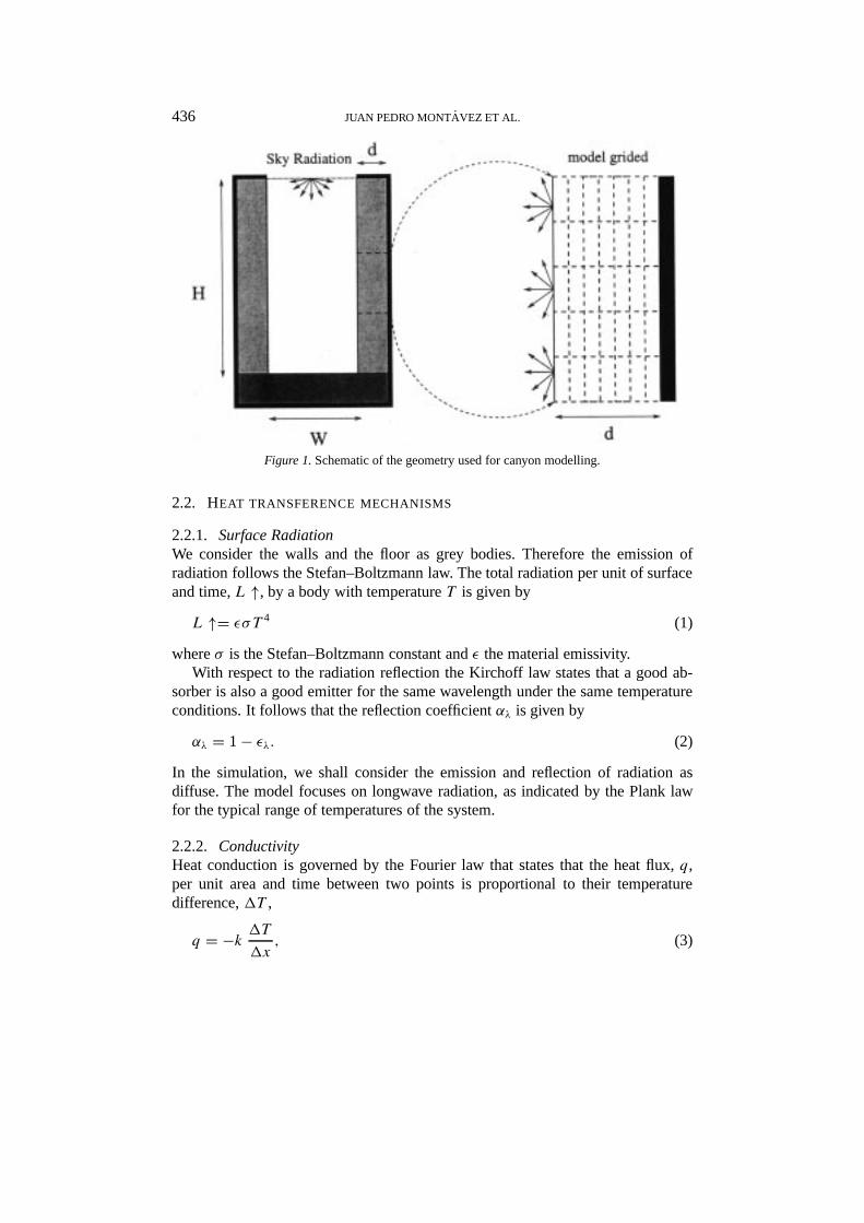
The system considered here is an infinite canyon of heightH , widthW and walls ofwidthd (Figure 1). The model is formulated for night time conditions. We also con-sider homogeneous and dry surfaces. This last requirement avoids possible effectsof latent heat transference which will not be taken into account. We assume thatwalls and ground can only lose energy through their exterior surface, i.e., interiorparts of these slices are thermally isolated. Finally, it is assumed no heat loss tooutside the canyon through convection.

Such an infinite canyon structure has been employed previously by other au-thors, e.g., Johnson et al. (1991), Arnfield and Mills (1994), Sakakibara (1996).An analysis of the errors due to considering the streets as infinite can be found inMontávez et al. (1998). The atmospheric conditions of clear skies and weak winds,which are assumed in this work, maximize the heat island intensity of the near–surface layer (Landsberg, 1981; Oke, 1987; Johnson et al., 1991; Montávez et al.,1999).

436 JUAN PEDRO MONT́AVEZ ET AL.

Figure 1.Schematic of the geometry used for canyon modelling.

2.2. HEAT TRANSFERENCE MECHANISMS

2.2.1. Surface RadiationWe consider the walls and the floor as grey bodies. Therefore the emission ofradiation follows the Stefan–Boltzmann law. The total radiation per unit of surfaceand time,L ↑, by a body with temperatureT is given by

L ↑= εσT 4 (1)

whereσ is the Stefan–Boltzmann constant andε the material emissivity.With respect to the radiation reflection the Kirchoff law states that a good ab-

sorber is also a good emitter for the same wavelength under the same temperatureconditions. It follows that the reflection coefficientαλ is given by

αλ = 1− ελ. (2)

In the simulation, we shall consider the emission and reflection of radiation asdiffuse. The model focuses on longwave radiation, as indicated by the Plank lawfor the typical range of temperatures of the system.

2.2.2. ConductivityHeat conduction is governed by the Fourier law that states that the heat flux,q,per unit area and time between two points is proportional to their temperaturedifference,1T ,

q = −k 1T1x

, (3)

NOCTURNAL SURFACE TEMPERATURES IN URBAN CANYONS 437

wherek is the thermal conductivity constant.

2.2.3. ConvectionDue to radiation mechanisms, canyon surfaces are not in thermal equilibrium withthe surrounding air, which induces a sensible heat flow between them. Observa-tional data at night time and calm conditions indicate that the air temperatureis almost homogeneous inside the canyon (Eliasson, 1996; Nakamura and Oke,1988). This is due to mechanisms of micro-advection and convection inside thecanyon. The heat transfer, q, between the surfaces and the surrounding air is thengiven by

q = hc(T − Ta), (4)

T being the temperature at a point surface of the canyon,Ta the air temperatureandhc is a constant which depends on the wind velocity in the canyonvc. For thiswe use the empirical formula (Mills, 1993),hc = 11.8+ 4.2vc (W m−2 K−1).

2.2.4. Sky RadiationIn the present model, when it is not known, the amount of sky radiation is calculatedby the empirical formula, (Oke, 1987)

L↓(0)= εa(0)σT 4a (5)

whereTa is the air temperature andεa(0) the atmospheric emission coefficient forcloudless skies, which is calculated by means of Idso’s formula (Idso, 1981). Thesky radiation is considered as diffuse. In this work we shall only consider clearsky conditions. The generalization to cloudy conditions is straightforward by cal-culating the corresponding atmospheric emission coefficient as indicated in Oke(1987).

2.3. MONTE CARLO SIMULATION

Before performing the simulation, the walls and floor of the canyon are discretizedin slices, whose size is taken to be small enough to assume uniform temperaturewithin each of them. As we are considering conduction inside the walls, the grid-ding must also be done in the direction perpendicular to the surfaces of the canyon(Figure 1). Initial conditions are imposed for the grid temperature distribution. Theeffect of different initial conditions is discussed in Section 4. The amount of energyexchanged in each step, that we shall call the energy unit (EU) must be fixed apriori. The grid size and the value of EU give rise to the finite size errors of themodel which shall be discussed in Section 3.

The simulation is performed by a long sequence of successive steps. Each stepconsists of an exchange of energy between two slices by means of any of themechanisms previously described. Below details are given how this is achieved.

438 JUAN PEDRO MONT́AVEZ ET AL.

2.3.1. Radiation SimulationA step of the radiation simulation is as follows: A slice of the canyon surface,which is randomly selected, emits an amount of energy given by Equation (1) bymeans of several ‘pencils’ of energy each of which carries one EU. The directionof the pencils must be determined. Since the canyon is infinite the problem can bereduced to two dimensions and the direction can be fixed by specifying the anglemade with the normal to the local surface. The diffuse emission condition implies aradiative intensity that varies with the cosine of that angle. Therefore the value forthe angle will be drawn from the cosine distribution in the interval [0, π ] following,for example, Kalos and Whitlock (1986).

Depending on its starting position and angle of emission, the energy carriedby the “pencil” can escape to the atmosphere or it can impinge into another slice.In the first case energy is lost. In the second one, the EU can either be absorbedor be reflected according to Equation (2). In terms of the Monte Carlo simulationthis means that we draw a random number from the uniform probability in theinterval [0, 1]. If that number is smaller thanαλ the energy is reflected, otherwiseit is absorbed. Multiple reflections are considered until the pencil is either ejectedto the atmosphere or absorbed by any slice. This algorithm is repeated for all thepencils required to complete the energy given by Equation (1).

The energy of an emitting slice must be diminished in a quantity equal to theamount of energy emitted, and the energy of an absorbing slice must be increasedby the energy of the absorbed pencils. Once this balance is finished, the temperatureof the pieces is updated according to

1T = 1U

V C(6)

1U and V being the increment of the energy and the volume of the piecerespectively, andC the heat capacity of the material.

It is worth mentioning that, as has been previously pointed out (Kobayashi andTakamura, 1994), multiple reflections will be relevant in the final results. We haveverified that the percentage of outgoing radiation in a canyon can be affected byapproximately 4% for an emissivity of 0.95 and up to 10% for 0.85. These numbersalso depend on theH/W ratio of the canyon, but this is the general relationship.

Regarding the simulation of the sky radiation, positions of the top of the canyonare selected randomly as emitter points with the same probability. The direction isselected as has been indicated above. The amount of EU generated depends onlyon the sky radiation flux.

2.3.2. Conduction SimulationThe basic ideas for simulating conduction by the Monte Carlo method are the sameones underlying the simulation of heat transfer by radiation. Obviously there aresome differences due to the fact that we are dealing with a different physical phe-nomenon. Now we have to consider only heat exchanges between two consecutive

NOCTURNAL SURFACE TEMPERATURES IN URBAN CANYONS 439

slices in the canyon. Let us note that they do not have to be surface slices becausethermal conduction inside the walls is also taken into account. Furthermore theenergy transfer is now governed by the Fourier law, Equation (3). In terms of theMonte Carlo simulation this means that the probability for heat transfer is differentfor each pair of slices. Thus the larger the temperature difference, the higher isthe probability for the heat transference. Hence we assign to each pair of adjacentslices a probability of being chosen proportional to the absolute value temperat-ure difference between both slices. Then we normalize that probability by makingequal to one the sum of all the probabilities to the number of adjacent slices. Atthis point a random number drawn from the uniform distribution in the interval [0,1] is generated and it is used to decide which pair of slices is chosen to performthe step. A step consists of a net heat flux from the hottest slice to the coolest one.Then the temperatures are updated by using Equation (6) and the step is concluded.

The amount of energy exchanged in each step is a model parameter that has tobe fixed a priori. As happens with the slice size, too large a value for this energy willgive rise to unacceptable large step errors in the final results, and too small a valuewill require very long simulations. In Section 3, we outline the criteria followed inthe present work to choose this parameter. Once its value has been fixed, the timeconsumed in each exchange,tf , is calculated from Equation (3).

Heat conductivity among parallel surface slices has almost no influence onthe final results. However, conduction inside the walls and floor is going to benecessary to obtain a good description of the temporal evolution of temperaturedistributions. Generalization for more complicated geometries and layered soilsand walls (e.g., Swaid, 1995) of canyons is straightforward.

2.3.3. Convection SimulationIn each step the air temperature is taken to be homogeneous in the canyon andequal to the average temperature of the canyon surfaces. As this process is a heatexchange by thermal conduction (between the air and the surfaces) the simulationis carried out as in the previous subsection. It is important to take this factor intoaccount when comparing with experimental data of surface temperature distribu-tion in the canyons. In general, the temperature distribution on canyon surfaces canbe reproduced approximately with a model without convection. The shape of thedistribution is reproduced but the results overestimate the experiment data (seeresults section). When convection is introduced into the model the quantitativeagreement is improved. The introduction of this physical effect does not modifythe energy budget of the canyon; it only rearranges the energy distribution.

2.3.4. CouplingSimulations clearly show that the time scales of these processes are quite differentand therefore they can be simulated independently of one another. Thus, after ac-tivating the radiation transfer during a given time the other processes are activated

440 JUAN PEDRO MONT́AVEZ ET AL.

sequentially for the same duration. In each time step, the order of simulation ofconduction and convection is randomly selected.

3. Numerical Test

Two ideal situations, for which analytical solutions are possible, have been simu-lated by the model. The accuracy of the Monte Carlo simulation has been studiedby comparing the results.

3.1. BLACK ADIABATIC CANYON

Firstly, we test the simulation of the thermal radiation. In this case, the idealsystem is a canyon with the geometry described before, plus the following extraassumptions:1. The surfaces are black bodies (ε = 1).2. All surfaces are at the same temperature because of the infinite thermal

conduction inside the canyon (k = ∞).3. There is no sky radiation (εa(0) = 0).

With those extra simplifications, it is possible (Montávez et al., 1998) to calculateanalytically the total energy emitted by the system and the outgoing radiation fromthe canyon by integrating (1). The percentage of lost energy in the canyon due toradiationξ , is given by:

ξ =(W +H)(π − 2tan−1(H

W))+ (W −H)ln(W 2+H 2)+Hln(H 2)−Wln(W 2)

π(2H +W)(7)

In Figure 2 we compare this value with the Monte Carlo prediction as it varieswith the ratioH/W . As we can see the agreement is remarkable. Such a simplifiedmodel explains qualitatively the effect of the canyon geometry in UHI formation.As the ratioH/W is increased the loss of energy is decreased, giving rise to aslower cooling. It also provides a theoretical justification (Montávez et al., 1998)of the logarithmic relationship obtained experimentally between the UHI intensityandH/W (Oke, 1981).

3.2. UNIDIMENSIONAL CONDUCTOR

The time evolution of the temperature distribution,T (x, x′; t), in an infiniteconductor in one dimension is given by

∂T (x, x′, t)∂t

= κ ∂2T (x, x′, t)∂x2

(8)

NOCTURNAL SURFACE TEMPERATURES IN URBAN CANYONS 441

Figure 2. Percentage of radiation lost for values of (H/W ). Line indicates analytical results andcircles are related to Monte Carlo results.

wherex andx′ are spatial coordinates,t the time andκ the thermal diffusivity. Ifwe take the initial condition

T (x, x′,0) = δ(x − x′) (9)

whereδ is Dirac’s delta function, the problem admits the following solution

T (x, x′, t) =√

1

4πκte−

14κt (x−x ′)2. (10)

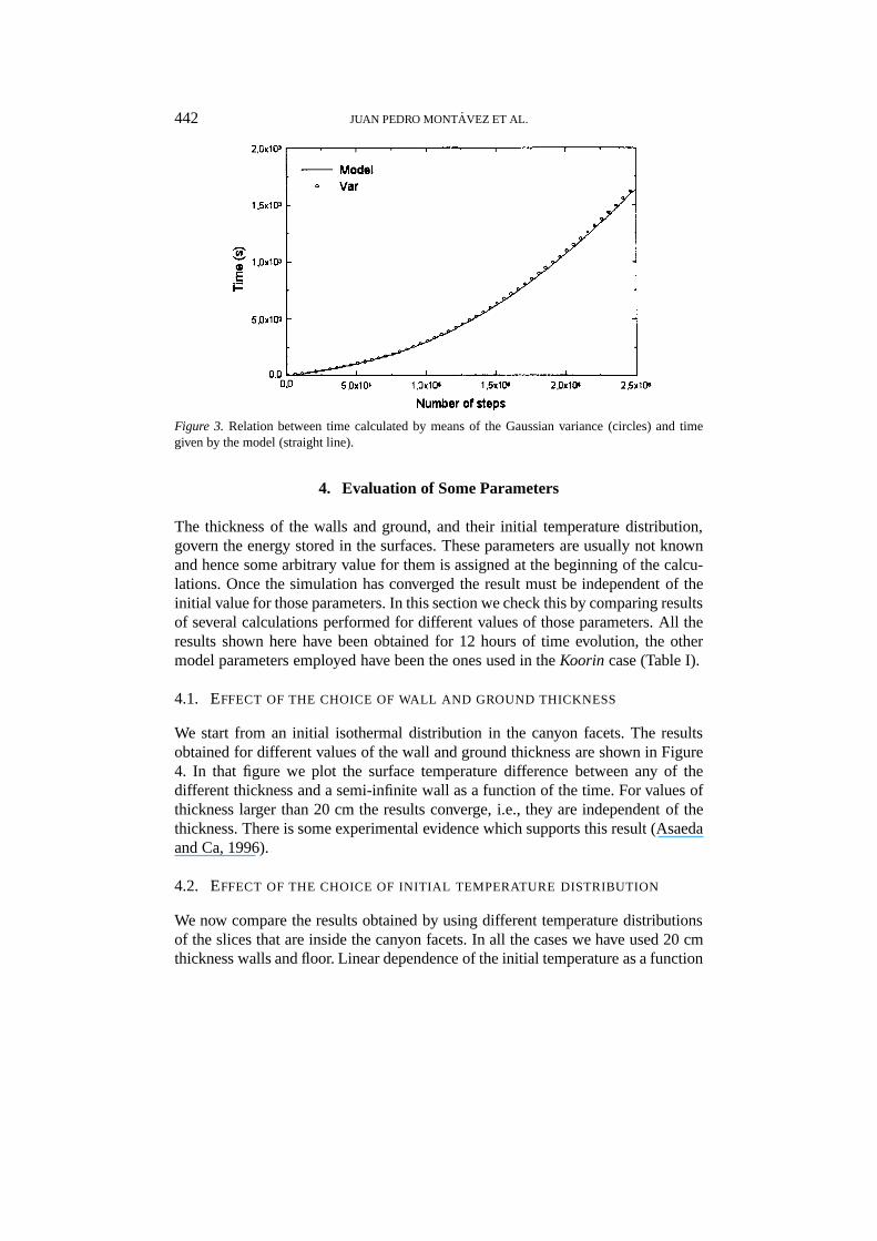
We have simulated this system with the Monte Carlo techniques described above.In doing so, the initial temperature distribution is selected to be Gaussian. Then,for several values of the number of steps, the model output was compared withthe theoretical Gaussian distribution. Its variance is given by the increment of timecorresponding to the number of steps performed. As we can see in Figure 3, aperfect agreement between the numerical and analytical results is obtained.

The agreement between simulation and analytical solutions indicates that thephysical processes are well simulated and provides a criterion to choose someparameters of the model. The selection of EU is done for each geometry takinginto account that the error relative to the analytical solution, increases with EU. Inthe case of conduction choosing the error in time and EU, we obtain slice size.

An example of typical values for the discretization are the following. For a 5-mwide canyon and 5-m height with 25-cm facet thickness, the length of the radiativesurface is 10 cm, and the perpendicular to the canyon facets gridding is 1 cm. TheEU for radiation and conduction was 1 J. With those input values the error in thetime and in the outgoing radiation is less than 0.2% and 2% respectively for asimulation corresponding to a 10-hour evolution.

442 JUAN PEDRO MONT́AVEZ ET AL.

Figure 3. Relation between time calculated by means of the Gaussian variance (circles) and timegiven by the model (straight line).

4. Evaluation of Some Parameters

The thickness of the walls and ground, and their initial temperature distribution,govern the energy stored in the surfaces. These parameters are usually not knownand hence some arbitrary value for them is assigned at the beginning of the calcu-lations. Once the simulation has converged the result must be independent of theinitial value for those parameters. In this section we check this by comparing resultsof several calculations performed for different values of those parameters. All theresults shown here have been obtained for 12 hours of time evolution, the othermodel parameters employed have been the ones used in theKoorin case (Table I).

4.1. EFFECT OF THE CHOICE OF WALL AND GROUND THICKNESS

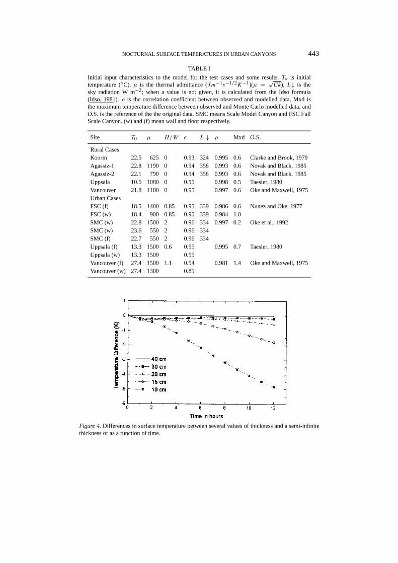
We start from an initial isothermal distribution in the canyon facets. The resultsobtained for different values of the wall and ground thickness are shown in Figure4. In that figure we plot the surface temperature difference between any of thedifferent thickness and a semi-infinite wall as a function of the time. For values ofthickness larger than 20 cm the results converge, i.e., they are independent of thethickness. There is some experimental evidence which supports this result (Asaedaand Ca, 1996).

4.2. EFFECT OF THE CHOICE OF INITIAL TEMPERATURE DISTRIBUTION

We now compare the results obtained by using different temperature distributionsof the slices that are inside the canyon facets. In all the cases we have used 20 cmthickness walls and floor. Linear dependence of the initial temperature as a function

NOCTURNAL SURFACE TEMPERATURES IN URBAN CANYONS 443

TABLE I

Initial input characteristics to the model for the test cases and some results.To is initialtemperature (◦C). µ is the thermal admittance (Jm−1s−1/2K−1)(µ = √Ck), L↓ is thesky radiation W m−2; when a value is not given, it is calculated from the Idso formula(Idso, 1981).ρ is the correlation coefficient between observed and modelled data, Mxd isthe maximum temperature difference between observed and Monte Carlo modelled data, andO.S. is the reference of the the original data. SMC means Scale Model Canyon and FSC FullScale Canyon. (w) and (f) mean wall and floor respectively.

Site T0 µ H/W ε L ↓ ρ Mxd O.S.

Rural CasesKoorin 22.5 625 0 0.93 324 0.995 0.6 Clarke and Brook, 1979Agassiz-1 22.8 1190 0 0.94 358 0.993 0.6 Novak and Black, 1985Agassiz-2 22.1 790 0 0.94 358 0.993 0.6 Novak and Black, 1985Uppsala 10.5 1080 0 0.95 0.998 0.5 Taesler, 1980Vancouver 21.8 1100 0 0.95 0.997 0.6 Oke and Maxwell, 1975Urban CasesFSC (f) 18.5 1400 0.85 0.95 339 0.986 0.6 Nunez and Oke, 1977FSC (w) 18.4 900 0.85 0.90 339 0.984 1.0SMC (w) 22.8 1500 2 0.96 334 0.997 0.2 Oke et al., 1992SMC (w) 23.6 550 2 0.96 334SMC (f) 22.7 550 2 0.96 334Uppsala (f) 13.3 1500 0.6 0.95 0.995 0.7 Taesler, 1980Uppsala (w) 13.3 1500 0.95Vancouver (f) 27.4 1500 1.1 0.94 0.981 1.4 Oke and Maxwell, 1975Vancouver (w) 27.4 1300 0.85

Figure 4.Differences in surface temperature between several values of thickness and a semi-infinitethickness of as a function of time.

444 JUAN PEDRO MONT́AVEZ ET AL.

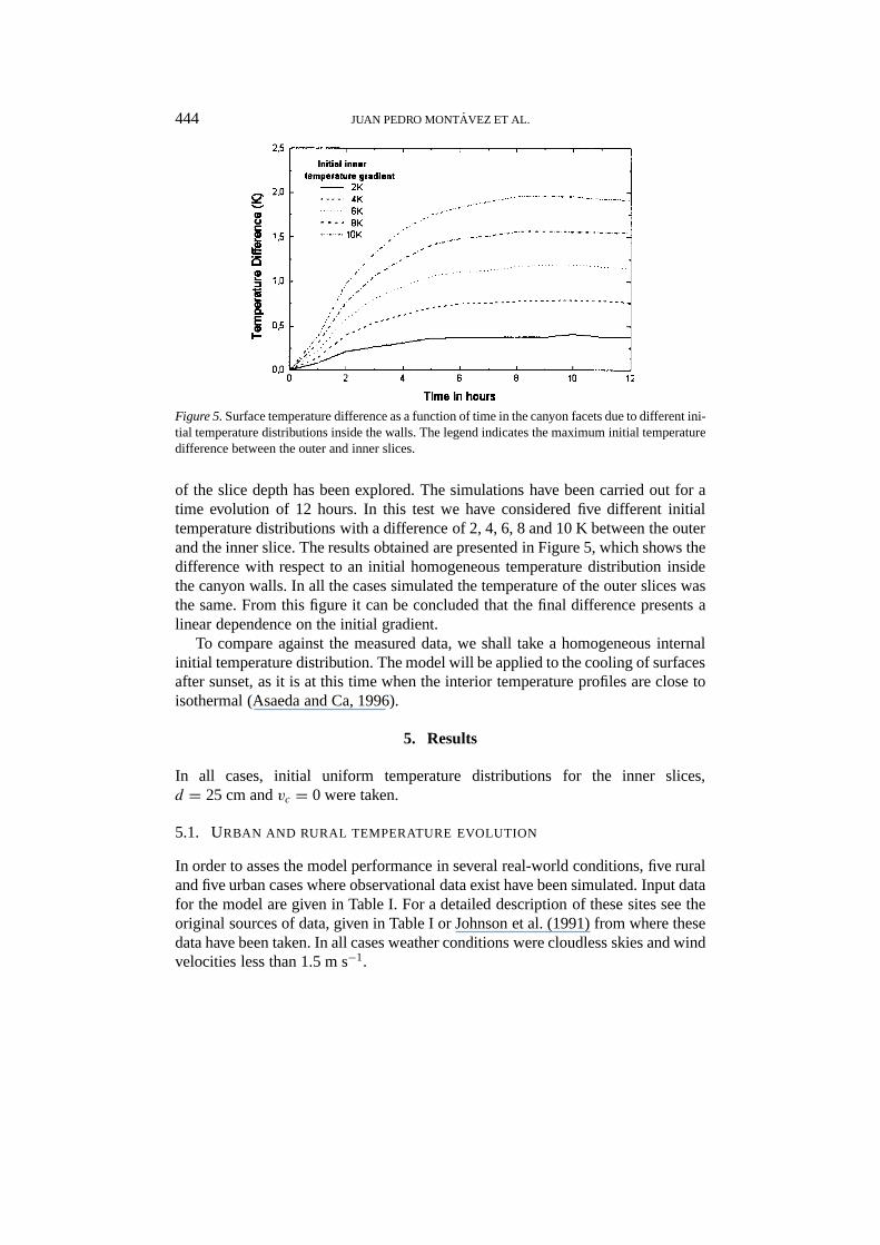
Figure 5.Surface temperature difference as a function of time in the canyon facets due to different ini-tial temperature distributions inside the walls. The legend indicates the maximum initial temperaturedifference between the outer and inner slices.

of the slice depth has been explored. The simulations have been carried out for atime evolution of 12 hours. In this test we have considered five different initialtemperature distributions with a difference of 2, 4, 6, 8 and 10 K between the outerand the inner slice. The results obtained are presented in Figure 5, which shows thedifference with respect to an initial homogeneous temperature distribution insidethe canyon walls. In all the cases simulated the temperature of the outer slices wasthe same. From this figure it can be concluded that the final difference presents alinear dependence on the initial gradient.

To compare against the measured data, we shall take a homogeneous internalinitial temperature distribution. The model will be applied to the cooling of surfacesafter sunset, as it is at this time when the interior temperature profiles are close toisothermal (Asaeda and Ca, 1996).

5. Results

In all cases, initial uniform temperature distributions for the inner slices,d = 25 cm andvc = 0 were taken.

5.1. URBAN AND RURAL TEMPERATURE EVOLUTION

In order to asses the model performance in several real-world conditions, five ruraland five urban cases where observational data exist have been simulated. Input datafor the model are given in Table I. For a detailed description of these sites see theoriginal sources of data, given in Table I or Johnson et al. (1991) from where thesedata have been taken. In all cases weather conditions were cloudless skies and windvelocities less than 1.5 m s−1.

NOCTURNAL SURFACE TEMPERATURES IN URBAN CANYONS 445

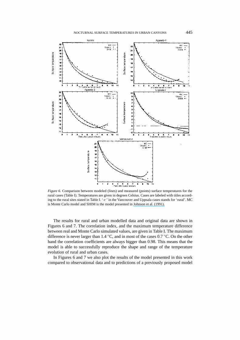
Figure 6.Comparison between modeled (lines) and measured (points) surface temperatures for therural cases (Table I). Temperatures are given in degrees Celsius. Cases are labeled with titles accord-ing to the rural sites stated in Table I. ‘-r ’ in the Vancouver and Uppsala cases stands for ‘rural’. MCis Monte Carlo model and SHIM is the model presented in Johnson et al. (1991).

The results for rural and urban modelled data and original data are shown inFigures 6 and 7. The correlation index, and the maximum temperature differencebetween real and Monte Carlo simulated values, are given in Table I. The maximumdifference is never larger than 1.4◦C, and in most of the cases 0.7◦C. On the otherhand the correlation coefficients are always bigger than 0.98. This means that themodel is able to successfully reproduce the shape and range of the temperatureevolution of rural and urban cases.

In Figures 6 and 7 we also plot the results of the model presented in this workcompared to observational data and to predictions of a previously proposed model

446 JUAN PEDRO MONT́AVEZ ET AL.

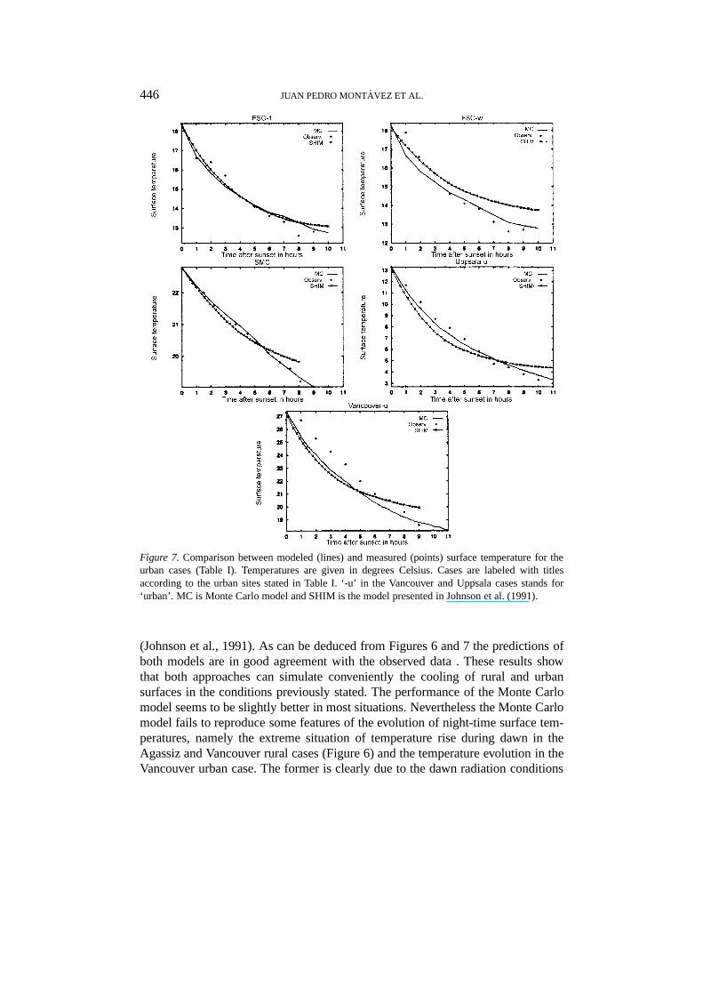
Figure 7. Comparison between modeled (lines) and measured (points) surface temperature for theurban cases (Table I). Temperatures are given in degrees Celsius. Cases are labeled with titlesaccording to the urban sites stated in Table I. ‘-u’ in the Vancouver and Uppsala cases stands for‘urban’. MC is Monte Carlo model and SHIM is the model presented in Johnson et al. (1991).

(Johnson et al., 1991). As can be deduced from Figures 6 and 7 the predictions ofboth models are in good agreement with the observed data . These results showthat both approaches can simulate conveniently the cooling of rural and urbansurfaces in the conditions previously stated. The performance of the Monte Carlomodel seems to be slightly better in most situations. Nevertheless the Monte Carlomodel fails to reproduce some features of the evolution of night-time surface tem-peratures, namely the extreme situation of temperature rise during dawn in theAgassiz and Vancouver rural cases (Figure 6) and the temperature evolution in theVancouver urban case. The former is clearly due to the dawn radiation conditions

NOCTURNAL SURFACE TEMPERATURES IN URBAN CANYONS 447

TABLE II

Surface and air temperatures recorded on two nights. Day 1 was the night of 27–28 of October1998 at 0130 LST and day 2 was the night of 11–12 of November 1998 at 0130 LST. Capitalletters indicate points of transversal sections, and the others indicate longitudinal sections. Themeasurement points are marked on Figure 8. The last line indicates the variation range of airtemperature in both streets. All data are given in degrees Celsius.

Transverse sections Longitudinal sectionsDay 1 Day 2 Day 1 Day 2

Sec 1 Sec 2 Sec 1 Sec 2 Lon 1 Lon 2 Lon 1 Lon 2

a 14 17 8 10 13 16 5 8 Ab 14 18 8 11 14 16 5 8 Bc 13 17 6 10 13 16 5 8 Cd 13 16 5 8 13 14 5 6 De 13 17 7 10 12 12 4 4 Ef 14 18 8 11 13 13 5 5 Fg 14 17 7 10 13 13 5 8 G

Ta 12.8–13 3.5–3.7 12.8–13 3.5–3.7 Ta

not being simulated by the Monte Carlo model; the latter has not been checked bythe authors in this study.

As we can see from Figures 6 and 7, the cooling is smaller in urban areas due inpart to the effect of geometry, which gives rise to the UHI formation. This geometryeffect is included in the simplified model of theblack adiabatic canyondescribedabove. Although it provided a qualitatively correct description of the phenomenon,it is too crude to give good quantitative agreement. Thus it is necessary to takeinto account all the heat transference mechanisms described above in order to fitthe experimental data. The heat conduction tends to re-establish the thermal equi-librium which was broken by the heat radiation. The effect of convection on thetemperature distribution on facets is to reduce the temperature differences betweenthe different points of the canyon caused by the radiation process. Finally the effectof parallel conduction is almost negligible. With respect to the heat radiation, wehave found that it is important to take into account the effect of multiple reflectionsin urban canyons because these can modify the results roughly by approximately10% in the difference between initial and final simulation temperature.

5.2. TEMPERATURE DISTRIBUTION ON CANYON FACETS

A temperature gradient is generated among the different surface points of thecanyon as a consequence of the energy transference mechanisms. The model pre-dicts that the canyon corners are warmer than the canyon centre. This is caused byradiation. In fact, a qualitatively equal result is found when only the exchange of

448 JUAN PEDRO MONT́AVEZ ET AL.

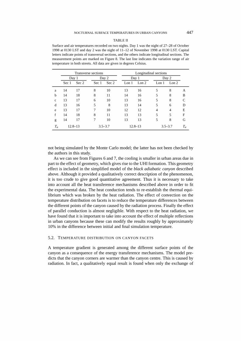
Figure 8.(a) Map of the site and points where measurements were taken. (b) Sections points.

heat by radiation is allowed. The effect of the other energy exchanges is to reducethe magnitude of the gradient.

To verify this phenomenon a measurement campaign was carried out. Surfacetemperatures were measured using an Infrared Thermometer Digitron model D202,and air temperatures with a digital Crison 638 Pt thermometer, which have instru-mental errors of±1 K and±0.1 K respectively. A map of the streets where thetemperatures were measured is shown in Figure 8. In the area selected for the meas-urements the height of the buildings is uniform; only the street width varies. Hencetemperature profiles for different values of the ratioH/W were obtained. Figure8 shows the points where the surface temperature measurements were performedand the results are given in Table II. The air temperatures were taken at levels from20 cm to 250 cm at several points in the streets. They were obtained by measuringduring two days with weather conditions of clear sky and weak winds.

The measured temperatures confirm the model prediction. Temperature dif-ferences between the centre and the corner inside a canyon of up to 4◦C werefound. These temperature differences increase slightly when the ratioH/W in-creases. Conversely, although air temperatures observed are almost homogeneous,the differences of surface temperature between points of both canyons reach up to4 ◦C (Table II). It should be mentioned that, in agreement with Eliasson (1996),the coldest point is found in the crossing point of the streets. This indicates theimportance of urban geometry on surface temperature evolution and therefore inthe UHI formation.

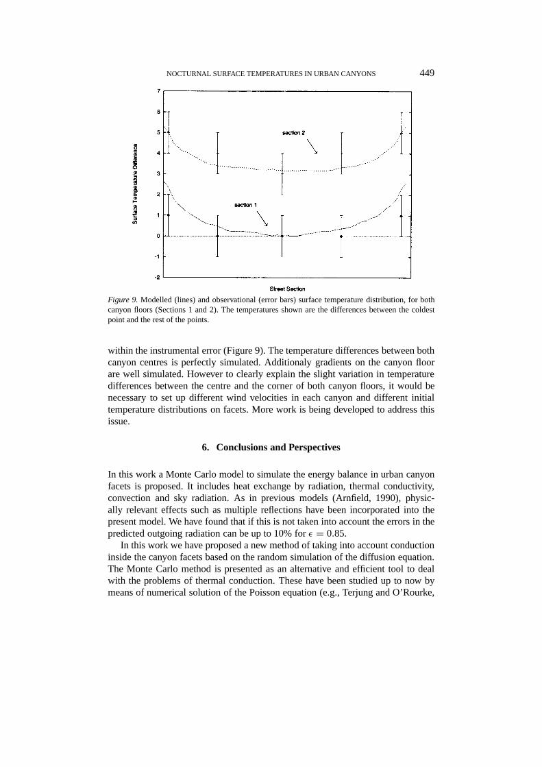
Although no initial conditions are known, in order to confirm these observa-tional results the model was applied to cases with the same geometric conditions,H/W = 1 for section 1 andH/W = 3 for section 2. The material features usedwere the same as those used in the case of Vancouver (urban) given in Table I. Theinitial temperature distribution on canyon facets was set to be homogeneous. In Fig-ure 9 the temperature differences between the coldest point, i.e., pointd of section1, in modelled and observational data for day 1 (Table II) and the rest of the pointsis represented. The theoretical prediction agrees with these observational results

NOCTURNAL SURFACE TEMPERATURES IN URBAN CANYONS 449

Figure 9.Modelled (lines) and observational (error bars) surface temperature distribution, for bothcanyon floors (Sections 1 and 2). The temperatures shown are the differences between the coldestpoint and the rest of the points.

within the instrumental error (Figure 9). The temperature differences between bothcanyon centres is perfectly simulated. Additionaly gradients on the canyon floorare well simulated. However to clearly explain the slight variation in temperaturedifferences between the centre and the corner of both canyon floors, it would benecessary to set up different wind velocities in each canyon and different initialtemperature distributions on facets. More work is being developed to address thisissue.

6. Conclusions and Perspectives

In this work a Monte Carlo model to simulate the energy balance in urban canyonfacets is proposed. It includes heat exchange by radiation, thermal conductivity,convection and sky radiation. As in previous models (Arnfield, 1990), physic-ally relevant effects such as multiple reflections have been incorporated into thepresent model. We have found that if this is not taken into account the errors in thepredicted outgoing radiation can be up to 10% forε = 0.85.

In this work we have proposed a new method of taking into account conductioninside the canyon facets based on the random simulation of the diffusion equation.The Monte Carlo method is presented as an alternative and efficient tool to dealwith the problems of thermal conduction. These have been studied up to now bymeans of numerical solution of the Poisson equation (e.g., Terjung and O’Rourke,

450 JUAN PEDRO MONT́AVEZ ET AL.

1979; Johnson et al., 1991) and the so called Force Restore Method (e.g., Johnsonet al., 1991; Swaid, 1995).

The effect of the subjective parameters (i.e., parameters that usually are notknown) in the model such as internal temperature profiles and thickness of wallsand ground have been evaluated, concluding that plane profiles are a good approx-imation in this case, and the results are unaffected when thicknesses are larger than20 cm.

Tests on the performance of the model show that it successfully simulates thecooling of rural and urban surfaces based on comparison of the output againstresults from independent field studies. An interesting output of the model is thetemperature distribution of the canyon surfaces. The results indicate that cornersare warmer than the central part of the canyon by up to several degrees in the samestreet. This effect has been observed experimentally, obtaining a good agreementwith the theoretical prediction.

Work is underway to extend the model to the three-dimensional case. First res-ults in the study of the temperature gradient in a street crossing have been obtained(Montávez et al., 1998).

Acknowledgements

The authors wish to thank Prof. E. Buendía for many valuable discussions, andDr. Eduardo Zorita and Dr. Julie Jones for carefully reading the text. This workhas been partially supported by the Spanish Dirección General de Investiga-ción Científica y Técnica (DGICYT) under contract CLI96-1871-c04-01. A.S.acknowledges the Spanish Ministerio de Educacíon y Cultura for a postdoctoralfellowship.

References

Arnfield, A. J.: 1990, ‘Canyon Geometry, the Urban Fabric and Nocturnal Cooling: A SimulationApproach’,Physical Geog.11, 220–239.

Arnfield, A. J. and Mills, G. M.: 1994, ‘An Analysis of the Circulation Characteristics and EnergyBudget of a Dry, Asymmetric, East-West Canyon. II Energy Budget’,Int. J. Climatol.14, 239–261.

Asaeda, T. and Ca, V. T.: 1996, ‘Heat Storage of Pavement and its Effect on the Lower Atmosphere’,Atmos. Environ.30, 413–427.

Binder, K.: 1992,The Monte Carlo Method in Condensed Matter Physics, Springer Verlag, Berlin,392 pp.

Bornstein, R.: 1982, ‘Urban Climate Models, Nature Limitations and Applications’,Proc. TechnicalConf. Mexico, WMO672, 237–276.

Cermak, J. E.: 1995, ‘Thermal Effects on Flow and Dispersion over Urban Areas: Capabilities forPrediction by Physical Modeling’,Atmos. Environ.30, 393–401.

Clarke, R. H. and Brook., R. (eds.): 1979,The Koorin Expedition: Atmospheric Boundary LayerData over Tropical Savannah Land, Australian Govt. Publishing Service, Dept. Sci., BureauMeteorol., 359 pp.

NOCTURNAL SURFACE TEMPERATURES IN URBAN CANYONS 451

Eliasson, Y.: 1996, ‘Urban Nocturnal Temperatures, Street Geometry and Land Use’,Atmos. Environ.30, 379–392.

Fernández, F. and Gómez, A. (eds.): 1998,Clima y Ambiente Urbano en Ciudades Españolas eIberoamericas. Parteluz, Madrid, 606 pp.

Figueroa, P. I. and Mazzeo, N. A.: 1998, ‘Urban-Rural Temperature Differences in Buenos Aires’,Int. J. Climatol.18, 1709–1723.

Gallo, K. P., Mcnab, A. L., Karl, T. R., Brown, J., Hood, J. J., and Tarpley, J. D.: 1993, ‘The Useof NOAA AVHRR Data for Assessment of the Urban Heat Island Effect’,J. Appl. Meteorol.32,899–908.

Idso, S. B.: 1981, ‘A Set of Equations for Full Spectrum and 8–14µm and 10.5–12.5µ ThermalRadiation from Cloudless Skies’,Water Resour. Res.17, 295–304.

Johnson, G. T., Oke, T. R., Steyn, D. G., Watson, I. D., and Voogt, J. A.: 1991, ‘Simulation ofSurface Urban Heat Island under “Ideal” Conditions at Night. Part 1, Theory and Tests againstField Data’,Boundary-Layer Meteorol.56, 275–294.

Jones, P. D., Groisman, P. Y., Coughlan, M., Plummer, N., Wong, W. C., and Karl, T. R.: 1990,‘Assessment of Urbanization Effects in Time Series of Surface Air Temperature over Land’,Nature347, 169–177.

Kalos, M. H. and Whitlock, P. A.: 1986,Monte Carlo Methods, Vol. I: Basics. Wiley, New York,186 pp.

Kobayashi, T. and Takamura, T.: 1994, ‘Upward Long Wave Radiation From a Non-Black UrbanCanopy’,Boundary-Layer Meteorol.69, 201–213.

Landsberg, H. E.: 1981,The Urban Climate, Academic Press, New York, 275 pp.Lee, H. Y.: 1988, ‘An Application of NOAA AVHRR Thermal Data to the Study of the Urban Heat

Island’,Atmos. Environ.27B, 1699–1720.Lester, W. A. (ed.): 1997,Recents Advances in Quantum Monte Carlo Methods, World Scientific,

Singapore, 235 pp.López, A., Fernández, F., Arroyo, F., Martin-Vide, J., and Cuadrat, J.: 1993,El Clima de las Ciudades

Españolas. Ed. Madrid, Madrid, 265 pp.Lu, J., Arya, P., Snyder, W. H., and Lawson, R. E.: 1997, ‘A Laboratory Study of the Urban Heat

Island in a Calm and Stably Stratified Environment. Part II: Velocity Field’,J. Appl. Meteorol.36, 1392–1402.

Mills, G. M.: 1993, ‘Simulation of the Energy Budget of a Urban Canyon. I Model Structure andSensitivity Test’,Atmos. Environ.27B, 157–170.

Mills, G. M. and Arnfield, A. J.: 1993, ‘Simulation of the Energy Budget of a Urban Canyon. IIComparison of Model Results with Measurements’,Atmos. Environ.27B, 171–181.

Montávez, J. P., Rodríguez, A. J., and Jiménez, J. I.: 1999, ‘A Study of the Urban Heat Island ofGranada’,Int. J. Climatol., in press.

Montávez, J. P., Sarsa, A., Sánchez, E., and Jiménez, J. I.: 1998,Applied Sciences and the En-vironment, Vol. 4 of Environmental Engineering, Chapter: Some Applications of Monte CarloMethods in Urban Climate, WIT Press, pp. 113–121.

Moreno, M. C.: 1994, ‘Intensity and Form of the Urban Heat Island in Barcelona’,Int. J. Climatol.14, 705–710.

Nakamura, Y. and Oke, T. R.: 1988, ‘Wind, Temperature and Stability Conditions in an East-WestOriented Urban Canyon’,Atmos. Environ.22, 2691–2700.

Noto, K.: 1996, ‘Dependence of the Heat Island Phenomena on Stable Stratification and HeatQuantity in a Calm Environment’,Atmos. Environ.30, 475–485.

Novak, M. D. and Black, T. A.: 1985, ‘Theorical Determination of the Surface Energy Balance andThermal Regimes of Bare Soils’,Boundary-Layer Meteorol.33, 313–333.

Nunez, M. and Oke, T. R.: 1977, ‘Energy Balance of an Urban Canyon’,J. Appl. Meteorol.16, 11–19.Oke, T. R.: 1981, ‘Canyon Geometry and the Nocturnal Urban Heat Island: Comparison of Scale

Model and Field Observations’,J. Climatol.1, 237–254.

452 JUAN PEDRO MONT́AVEZ ET AL.

Oke, T. R.: 1987,Boundary Layer Climates, Routledge, London and New York, 435 pp.Oke, T. R. and Maxwell, G. B.: 1975, ‘Urban Heat Island Dynamics in Montreal and Vancouver’,

Atmos. Environ.9, 191–200.Oke, T., Johnson, G., Steyn, D., and Watson, I.: 1991, ‘Simulation of Surface Urban Heat Island under

“Ideal” Conditions. Part 2: Diagnosis of Causation’,Boundary-Layer Meteorol.56, 339–358.Oke, T. R., Zeuner, G., and Jauregui, E.: 1992, ‘The Surface Energy Balance in Mexico City’,Atmos.

Environ.26B, 433–444.Roth, H., Oke, T. R., and Emery, W. J.: 1984, ‘Satellite-derived Urban Heat Islands from Three

Coastal Cities and the Utilization of Such Data in Urban Climatology’,Int. J. Remote Sens.10,1–13.

Saitoh, T. S., Shimada, T., and Hoshi, H.: 1996, ‘Modeling and Simulation of the Tokyo Urban HeatIsland’,Atmos. Environ.30, 3431–3442.

Sakakibara, Y.: 1996, ‘A Numerical Study of the Effect of Urban Geometry upon the Surface EnergyBudget’,Atmos. Environ.30, 487–496.

Swaid, H.: 1995, ‘Urban Related Aspects of the Force-Restore Method’,Atmos. Environ.29, 3401–3409.

Taesler, R.: 1980, ‘Studies of the Development and Thermal Structure of the Urban Boundary Layerin Uppsala: Parts I and II’, Reports 60 and 61, Meteorol. Inst. Uppsala Univ.

Terjung, W. H. and O’Rourke, P. A.: 1979, ‘Simulating the Causal Elements of Urban Heat Islands’,Boundary-Layer Meteorol.19, 93–118.

Voogt, J. A. and Oke, T. R.: 1991, ‘Validation of an Urban Radiation Model for Nocturnal Long-WaveFluxes’,Boundary-Layer Meteorol.54, 347–361.

Yague, C., Zurita, E., and Martínez, A.: 1996, ‘Statistical Analysis of the Urban Heat Island’,Atmos.Environ.30, 429–435.