STRUCTURAL ANALYSIS OF SUBMARINE PIPELINES ...
340
STRUCTURAL ANALYSIS OF SUBMARINE PIPELINES UNDER SUBMARINE SLIDE AND THERMAL LOADING By INDRANIL GUHA BE (Mech), M. Tech (Pipeline), MIEAust, CPEng, NER THE UNIVERSITY OF WESTERN AUSTRALIA This thesis is presented for the degree of Doctor of Philosophy of The University of Western Australia Centre for Offshore Foundation Systems Ocean Graduate School August 2020
-
Upload
khangminh22 -
Category
Documents
-
view
0 -
download
0
Transcript of STRUCTURAL ANALYSIS OF SUBMARINE PIPELINES ...
STRUCTURAL ANALYSIS OF SUBMARINE
PIPELINES UNDER SUBMARINE SLIDE AND
THERMAL LOADING
By
INDRANIL GUHA
BE (Mech), M. Tech (Pipeline), MIEAust, CPEng, NER
THE UNIVERSITY OF WESTERN AUSTRALIA
This thesis is presented for the degree of
Doctor of Philosophy of
The University of Western Australia
Centre for Offshore Foundation Systems
Ocean Graduate School
August 2020


i
Thesis declaration
I, Indranil Guha, certify that:
This thesis has been substantially accomplished during enrolment in this degree.
This thesis does not contain material which has been submitted for the award of any other
degree or diploma in my name, in any university or other tertiary institution.
In the future, no part of this thesis will be used in a submission in my name, for any other
degree or diploma in any university or other tertiary institution without the prior approval
of The University of Western Australia and where applicable, any partner institution
responsible for the joint-award of this degree.
This thesis does not contain any material previously published or written by another
person, except where due reference has been made in the text and, where relevant, in the
Authorship Declaration that follows.
This thesis does not violate or infringe any copyright, trademark, patent, or other rights
whatsoever of any person.
This thesis contains published work and/or work prepared for publication, some of which
has been co-authored.
Signature:
Date: 13/08/2020

ii
Abstract
Pipelines are the safest, most reliable, economic and efficient means for the
transportation of petroleum fluids and water. In the last few decades, the importance of
the pipeline transportation system has increased significantly due to the hydrocarbon
industry developing resources that are further offshore. This thesis is concerned with the
structural behaviour of submarine pipelines subjected to submarine slide impact, and
thermal loading conditions.
The research has aimed to support the transition of oil and gas developments into
deeper water and more remote conditions. The principal motivations are the needs for (a)
export and tieback pipelines to negotiate regions of unstable or steeply sloping terrain,
where submarine slides may occur potentially impacting the pipeline; and (b) for high
temperature, high pressure, pipelines laid directly on the seabed in deep water to
withstand cycles of thermal and pressure loading during operation. Emphasis is placed
on the axial pipe-soil interaction and structural behaviour of the pipeline.
Analytical models are derived for the axial pipe-soil elastic stiffness and
numerical solutions using FE software ABAQUS are provided for axial, horizontal, and
vertical motions of a pipeline relative to the seabed with the aim of expressing these
parameters in terms of fundamental elastic properties of the soil. Where appropriate, the
theoretical techniques used for pile design are transferred to pipeline conditions to model
the axial slide loading condition. A parametric study of pipeline-slide interaction has
been carried out to provide insights into the dominant governing parameters and to assess
the sensitivity of the pipeline structural loading to the geotechnical (i.e. pipe-soil, slide
material) input parameters.
Thereafter, classical buckling theory has been extended to estimate the critical
lateral buckling load of on-bottom pipelines subjected to axial loading down-stream of
the submarine slide, incorporating the dominant governing geotechnical and as-laid
parameters, and to assess the sensitivity of the critical buckling load of the pipeline to
these input parameters.
Axial walking of deepwater pipelines due to thermal and pressure cycles during
their operational life is also addressed, extending the present theoretical framework by
incorporating the elastic-plastic (bi-linear) response of the soil into the analytical solution
and verifying the solution numerically. Furthermore, the walking behaviour of on-bottom
pipeline has been analysed using a velocity-dependent friction model within ABAQUS
to provide an equivalent friction factor that allows for this velocity-dependency via a
single value.

iii
Acknowledgement
I would like to thank my supervisors Prof David J White and Prof Mark F
Randolph for their guidance and support throughout the course of this research. I am
greatly indebted to both of them for their penetrating and timely criticisms. Without that,
many of the ideas of this thesis may have remained undeveloped. The research presented
here forms part of the activities of the Centre for Offshore Foundation Systems (COFS),
supported as a node of the Australian Research Council Centre of Excellence for
Geotechnical Science and Engineering (grant CE110001009) and through the Fugro
Chair in Geotechnics, the Lloyd’s Register Foundation Chair and Centre of Excellence
in Offshore Foundations and the Shell EMI Chair in Offshore Engineering.
I also owe much to my colleagues, staffs from IT and administration in the Centre
for Offshore Foundation System at the University of Western Australia for their constant
support and motivation.
I would also like to record my thanks to my wife Munmun Basak for her
continuing encouragement, love, sacrifice and support throughout the journey. She made
this journey easier for me. At the same time, I would like to thank my parents and in-
laws. Without their motivation, I could not have finished it.
Except where specific reference is made in the text to the work of others, the
contents of this dissertation are original and have not been submitted to any other
university.
“I am indebted to my father for living, but to my teacher for living well”
-Alexander the Great

iv
Authorship declaration: Co-authored publications
1. Guha, I., & Whitney, B. (2012). ‘Seismic vulnerability of Australian buried pipeline
industry’. In Proc of 11th Australia New Zealand Conference on Geomechanics (ANZ
2012), Melbourne, Australia.
This paper was based on the research proposal and chapters 1 and 2. Candidate
drafted the paper and second author Dr. Beau Whitney contributed to the final version.
2. Guha, I., Randolph, M.F., White, D.J. (2016). ‘Evaluation of elastic stiffness
parameters for pipeline-soil interaction', ASCE, Journal of Geotechnical and
Geoenvironmental Engineering, 142, 6.
DOI: 10.1061/(ASCE)GT.1943-5606.0001466
This paper was based on chapter 3. Candidate performed the analytical and numerical
modelling under the guidance of the co-authors. The candidate prepared the first draft
of the paper. Prof. Mark Randolph and Prof. David White reviewed and contributed
to the final version.
3. Guha, I., Randolph, M.F., & White, D.J., (2020). Analysis of axial response of
submarine pipeline to debris flow loading’. Accepted at Journal of Geotechnical and
Geoenvironmental Engineering, August 2020.
This paper was based on chapter 4. Candidate performed the analytical and numerical
modelling under the guidance of the co-authors. The candidate interpreted the results
reported in this paper. Prof. Mark Randolph prepared the first draft of the paper and
all authors revised and contributed to the final version.”
4. Guha, I., White, D.J., & Randolph, M.F (2020). ‘Parametric solution of lateral
buckling of submarine pipelines. Applied Ocean Research, 98.
https://doi.org/10.1016/j.apor.2020.102077
This paper was based on chapter 5. Candidate performed the analytical and numerical
modelling under the guidance of co-authors. The candidate prepared the first draft of
the paper. Prof. David White and Prof. Mark Randolph reviewed and contributed to
the final version.
5. Guha, I., White, D.J., & Randolph, M.F. (2018). ‘Subsea pipeline walking – the effect
of a bi-linear friction model’. Submitted at, ISFOG 2020.
This paper was based on chapter 6 and was accepted at OMAE 2019, but was
withdrawn (as none of the authors could attend) and resubmitted to ISFOG 2020.
Candidate performed the analytical and numerical modelling under the guidance of
co-authors. The candidate prepared the first draft of the paper. Prof. David White and
Prof. Mark Randolph reviewed and contributed to the final version.

v
6. Guha, I., White, D.J., & Randolph, M.F. (2018). ‘Subsea pipeline walking with
velocity dependent friction’, Applied Ocean Research, 82, January 2019, Pages 296-
308.
https://doi.org/10.1016/j.apor.2018.10.028
This paper was based on chapter 7. Candidate performed the analytical and numerical
modelling under the guidance of co-authors. The candidate prepared the first draft of
the paper. Prof. David White and Prof. Mark Randolph reviewed and contributed to
the final version.
Indranil Guha David J White Mark F Randolph
11th August 2020
11th August 2020
11th August 2020
Date Date
Date

Structural analysis of submarine pipelines
vi
Table of Content
INTRODUCTION ............................................................................... 1
OVERVIEW ............................................................................................................ 1
SUBMARINE PIPELINES ..................................................................................... 2
AUSTRALIAN OIL AND GAS DEVELOPMENT AND SUBMARINE
PIPELINES ............................................................................................................. 4
1.1 GEOTECHNICAL CHALLENGES .............................................................. 6
1.2 RESEARCH GOALS ...................................................................................... 7
1.3 THESIS OUTLINE ......................................................................................... 9
CURRENT METHODS USED FOR STRUCTURAL ANALYSIS
OF SUBMARINE PIPELINES ................................................................................ 17
2.1 OVERVIEW ................................................................................................... 17
2.2 STRUCTURAL ANALYSIS OF PIPELINES.................................................. 19
2.2.1 Submarine pipe-soil interaction ............................................................... 19
2.2.2 Geohazard – submarine slides ................................................................. 26
2.2.3 Lateral Buckling ...................................................................................... 35
2.2.4 Pipeline Walking ..................................................................................... 37
Axial pipe-soil interaction during walking ........................................................... 45
Pipeline walking and velocity dependent friction ................................................. 48
2.3 CONCLUSIONS ............................................................................................. 48
EVALUATION OF ELASTIC STIFFNESS PARAMETERS FOR
PIPELINE-SOIL INTERACTION .......................................................................... 63
3.1 OVERVIEW ................................................................................................... 63
3.2 PROBLEM DEFINITION AND NOTATIONS ............................................... 64
3.3 VERTICAL ELASTIC STIFFNESS ................................................................ 65
3.3.1 Rectangular ............................................................................................. 66
3.3.2 Circular ................................................................................................... 68
3.3.3 Strip ......................................................................................................... 68
3.3.4 Effect of embedment - rectangular ........................................................... 68
3.3.5 Pipe as half pile ....................................................................................... 69
3.3.6 Buried pipeline ........................................................................................ 70
3.3.7 Pipe on seabed – design guidelines .......................................................... 70
3.3.8 Non-homogeneous soil: ........................................................................... 71

Structural analysis of submarine pipelines
vii
3.4 HORIZONTAL (LATERAL) ELASTIC STIFFNESS ..................................... 71
3.4.1 Rectangular ............................................................................................. 72
3.4.2 Circular ................................................................................................... 73
3.4.3 Strip ........................................................................................................ 74
3.4.4 Pipe on seabed – design guideline ........................................................... 74
3.4.5 Effect of embedment ................................................................................ 74
which leads to a maximum increase by a factor of 1.33 compared with a surface
strip footing, for an embedment of w/B = 0.5. ...................................................... 75
3.4.6 Pipe as half pile ....................................................................................... 75
3.5 AXIAL ELASTIC STIFFNESS ....................................................................... 75
3.5.1 Rectangular ............................................................................................. 76
3.5.2 Embedment effect .................................................................................... 76
3.5.3 Pipeline as half pile ................................................................................. 77
3.5.4 Buried pipe .............................................................................................. 78
3.6 ANALYTICAL SOLUTION ........................................................................... 78
3.6.1 Axial load transfer stiffness of pipe on non-homogeneous seabed ............ 78
3.7 DISCUSSION ................................................................................................. 80
3.8 NUMERICAL SOLUTION ............................................................................. 83
3.8.1 Geometry and mesh ................................................................................. 83
3.8.2 Numerical analysis .................................................................................. 84
3.8.3 Verification of the model with V-H yield envelops .................................... 84
3.8.4 Parametric study ..................................................................................... 85
3.9 RELATION AMONGST AXIAL, VERTICAL AND LATERAL ELASTIC
STIFFNESSES OF ON-BOTTOM PIPELINE ........................................................ 86
3.9.1 Comparison of elastic stiffnesses ............................................................. 87
3.10 CONCLUSIONS ............................................................................................. 88
ANALYTICAL SOLUTION OF SUBMARINE PIPELINE AND
SLIDE INTERACTION ......................................................................................... 119
4.1 INTRODUCTION ........................................................................................ 119
4.2 PROBLEM DEFINITION AND BACKGROUND LITERATURE ............... 120
4.2.1 Active slide loading – geotechnical approach ........................................ 120
4.2.2 Passive loading ..................................................................................... 123
4.3 DERIVATION OF ANALYTICAL SOLUTION ........................................... 127

Structural analysis of submarine pipelines
viii
4.3.2 Input parameters and dimensionless groups........................................... 127
4.3.3 Elastic zone uC ≤ u ≤∞ ........................................................................... 129
4.3.4 Passive slide zone uB≤ u ≤ uC ................................................................. 131
4.3.5 Active slide zone uA≤ u ≤ uB ................................................................... 133
4.3.6 Summary of solution .............................................................................. 134
4.4 NON DIMENSIONAL DESIGN CHARTS ................................................... 135
4.4.1 Effect of slide force on pipe loading ....................................................... 136
4.4.2 Effect of slide force on passive length .................................................... 136
4.4.3 Effect of slide force on displacements..................................................... 137
4.5 DISCUSSION ............................................................................................... 137
4.5.1 Example cases ....................................................................................... 138
4.5.2 Numerical verification ........................................................................... 140
4.6 SENSITIVITY OF BUCKLING .................................................................... 141
4.7 CONCLUSIONS ........................................................................................... 142
PARAMETRIC SOLUTION OF LATERAL BUCKLING OF
SUBMARINE PIPELINES..................................................................................... 171
5.1 INTRODUCTION ......................................................................................... 171
5.2 PROBLEM DEFINITION AND NOTATIONS ............................................. 174
5.3 DIMENSIONAL ANALYSIS ....................................................................... 175
5.4 METHODOLOGY ........................................................................................ 178
5.4.2 Out-of-straightness (OOS) ..................................................................... 179
5.4.3 Lateral and axial soil response: stiffness and limiting resistance ........... 180
5.4.4 Numerical method.................................................................................. 182
5.4.5 Beam element as pipe model .................................................................. 185
5.4.6 Pipe-soil interaction model .................................................................... 187
5.4.7 Model discretization and boundary conditions ....................................... 188
5.5 CASE STUDY .............................................................................................. 189
5.5.2 Example analyses – effect of OOS .......................................................... 189
5.5.3 Example analyses – effect of soil resistance.......................................... 191
5.6 RESULTS OF PARAMETRIC STUDY ........................................................ 192
5.6.2 Without initial stress and axial spring .................................................... 193
5.6.3 Without initial stress and with axial spring ............................................ 193
5.6.4 With initial stress and axial springs ....................................................... 194

Structural analysis of submarine pipelines
ix
5.7 CONCLUSIONS ........................................................................................... 196
SUBSEA PIPELINE WALKING WITH A BI-LINEAR SEABED
MODEL ………………………………………………………………………...223
6.1 INTRODUCTION ........................................................................................ 223
6.2 EXISTING WALKING MODELS ................................................................ 224
6.2.2 SCR tension ........................................................................................... 225
6.2.3 Seabed slope .......................................................................................... 225
6.2.4 Thermal transients ................................................................................. 226
6.2.5 Liquid hold up ....................................................................................... 227
6.3 MODELLING ASSUMPTIONS ................................................................... 229
6.3.2 Analytical modelling .............................................................................. 230
6.3.3 Finite element modelling ....................................................................... 232
6.3.4 Model validation for flat seabed ............................................................ 233
6.4 NUMERICAL ANALYSIS OF WALKING .................................................. 235
6.4.2 SCR tension and rigid-plastic seabed ..................................................... 235
6.4.3 Seabed slope and rigid-plastic seabed ................................................... 237
6.4.4 Thermal transients and rigid-plastic seabed .......................................... 238
6.5 MODELLING OF MOBLISATION EFFECT ON WALKING, ELASTIC
PLASTIC SEABED .............................................................................................. 239
6.5.2 Approach ............................................................................................... 240
6.5.3 Numerical analysis ................................................................................ 240
6.5.4 Analytical solution ................................................................................. 241
6.6 CONCLUSIONS ........................................................................................... 246
SUBSEA PIPELINE WALKING WITH VELOCITY DEPENDENT
SEABED FRICTION ……………………………………………………………….271
7.1 INTRODUCTION ........................................................................................ 271
7.2 OBJECTIVE ................................................................................................. 273
7.3 VELOCITY DEPENDENT PIPE-SOIL RESISTANCE ................................ 274
7.3.1 Existing data ......................................................................................... 274
7.3.2 Representing present data with rate model ............................................ 275
7.4 NUMERICAL MODELLING WITH FRICTION RATE MODEL................ 275
7.4.1 Non-dimensional analysis ......................................................................... 276
7.4.1 Benchmarking case - single element test ................................................ 278
7.4.2 Benchmarking case – 2 km pipeline on flat seabed (β= 0) ...................... 279

Structural analysis of submarine pipelines
x
7.4.3 Walking due to SCR tension ................................................................... 281
7.4.4 Walking due to seabed slope .................................................................. 283
7.4.5 Walking due to thermal transients .......................................................... 284
7.4.6 Distributed displacements with rate model ............................................. 285
7.5 PARAMETRIC STUDY EXPLORING EQUIVALENT FRICTION ............. 286
7.5.2 SCR tension ........................................................................................... 287
7.5.3 Seabed slope .......................................................................................... 287
7.5.4 Thermal transients ................................................................................. 288
7.5.5 Equivalent friction factor ....................................................................... 288
7.5.6 Effect of time ratio Thc ............................................................................ 289
7.5.7 Effect of characteristic strain, εc ............................................................ 290
7.6 CONCLUSIONS ........................................................................................... 290
CONCLUSIONS AND FUTURE WORK ...................................... 317
OVERVIEW ......................................................................................................... 317
CONCLUDING REMARKS ................................................................................. 317
8.2.1 Elastic stiffness ...................................................................................... 317
8.2.2 Submarine slide pipeline interactions..................................................... 318
8.2.3 Lateral buckling of submarine pipelines................................................. 319
8.2.4 Submarine Pipeline Walking .................................................................. 320
FUTURE RESEARCH .......................................................................................... 321

Structural analysis of submarine pipelines
1
INTRODUCTION
OVERVIEW
Pipelines are the most safe, reliable, economic and efficient means for the transportation
of petroleum fluids and water. In the last few decades the importance of pipeline
transportation systems has increased significantly due to their extensive use in the
hydrocarbon industry. With increasing demand in the petroleum industry, new
developments of oil and gas infrastructure are moving towards deeper water. This
requires design and construction of long high temperature and high pressure pipelines
from deep sea to the shore. As a result, the cost of in-field flowlines and export pipelines
has increased significantly, leading to a paradigm shift in the importance of pipelines and
risers (Randolph and White, 2008a).
The first submarine pipeline was laid on the seabed in 1954. Since then offshore
production has reached water depths in excess of 2,100 m, and current exploration
has extended to almost 3,500 m depth (Kyriakides & Corona, 2007). Thousands
of kilometres of pipelines have already been laid onshore to meet the demand
supply gap for energy, and to transport water or sewage to maintain human
habitation throughout the land. Therefore, the onshore pipeline industry has
needed to meet challenges such as where pipelines cross earthquake prone zones,
traverse steep hill sides or in challenging regions such as the arctic. These threats
can be mitigated or minimised with optimal route selection, material selection
etc.

Structural analysis of submarine pipelines
2
However, the offshore industry is still evolving and with passing time new
challenges are revealed. These are instigating new technologies to investigate
and evaluate design methodologies for offshore pipelines (Bai, 2001).
SUBMARINE PIPELINES
Even though developing submarine pipeline infrastructure requires a significant capital
investment, most of the pipelines have a life span of more than 40 years and require
limited maintenance when designed and constructed effectively. In the past three decades,
significant hydrocarbon reserves have been identified offshore, including the North Sea,
the Gulf of Mexico, the Persian Gulf, offshore Brazil, West Africa, and more recently
fields in Malaysia, Indonesia, Northwest Australia, and in the Bay of Bengal of India (Bai,
2001).
As current hydrocarbon reserves are found in much deeper water, many hundreds of
kilometres of new submarine pipelines are being proposed to transport hydrocarbon fluids
from far field locations. In deepwater, seabed is comprised of finer-grained sediments
than typically encountered in shallow water. Also, hydrodynamic forces are much
reduced in deepwater, so that pipelines are generally laid directly on the seabed without
trenching or any other form of stabilisation. However, in deepwater other geotechnical
challenges need to be met, such as impact by submarine slides or operational challenges
such as cyclic expansion and contraction due to fluctuating temperatures and pressure. A
thorough introduction to these issues has been provided in relevant chapters of the
offshore geotechnical engineering books of Dean (2010) and Randolph and Gourvenec
(2011), and also in the papers of Cathie et al. (2005), White and Cathie (2010), Randolph
(2013), and the recently concluded JIP paper of White et al. (2016).

Structural analysis of submarine pipelines
3
Figure 1-1: Existing and proposed pipelines at the North West Shelf of Australia
In the case of deep-water pipelines, forces from hydrodynamic loading are
generally small and the dominant forces are from high internal temperature and pressure,
which tend to cause expansion (Bruton et al., 2008). Axial resistance between the pipe
and the seabed opposes this expansion. Excessive compressive forces lead to buckling,
but the buckling response depends critically on the lateral soil resistance. When buckling
occurs, it significantly reduces the net axial load in the pipe. On the other hand, excessive
buckling may lead to high bending strains in the pipe section. So, controlled buckling
(Figure 1-2) may be a feasible solution for relief of thermal loading. Accumulated axial
movement due to repeated thermal and pressure cycles may lead to global displacement
of pipes. This phenomenon is termed ‘walking’ (Carr et al., 2006). For design purposes,
it is very important to assess pipeline buckling and walking accurately. Recent design
approaches to control buckling and walking have necessitated predicting the available
soil resistance on pipelines undergoing movement, accounting for the associated changes
in seabed geometry and strength. The existing models are mainly derived for stability
Structural analysis of submarine pipelines
4
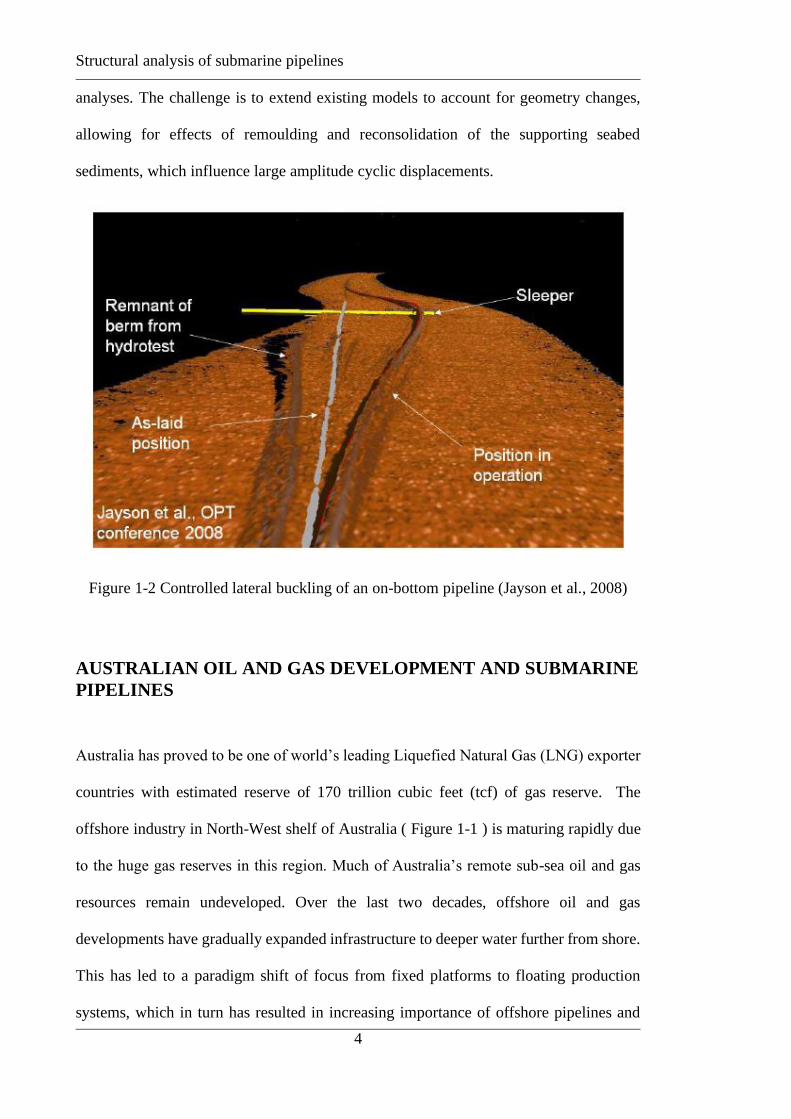
analyses. The challenge is to extend existing models to account for geometry changes,
allowing for effects of remoulding and reconsolidation of the supporting seabed
sediments, which influence large amplitude cyclic displacements.
Figure 1-2 Controlled lateral buckling of an on-bottom pipeline (Jayson et al., 2008)
AUSTRALIAN OIL AND GAS DEVELOPMENT AND SUBMARINE
PIPELINES
Australia has proved to be one of world’s leading Liquefied Natural Gas (LNG) exporter
countries with estimated reserve of 170 trillion cubic feet (tcf) of gas reserve. The
offshore industry in North-West shelf of Australia ( Figure 1-1 ) is maturing rapidly due
to the huge gas reserves in this region. Much of Australia’s remote sub-sea oil and gas
resources remain undeveloped. Over the last two decades, offshore oil and gas
developments have gradually expanded infrastructure to deeper water further from shore.
This has led to a paradigm shift of focus from fixed platforms to floating production
systems, which in turn has resulted in increasing importance of offshore pipelines and
Structural analysis of submarine pipelines
5
riser systems (Randolph & White, 2008a). Australia’s gas industry relies on ultra-long
sea-bed pipelines to bring the oil and gas from remote offshore hydrocarbon fields to
processing plants on shore.
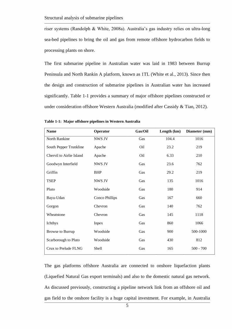
The first submarine pipeline in Australian water was laid in 1983 between Burrup
Peninsula and North Rankin A platform, known as 1TL (White et al., 2013). Since then
the design and construction of submarine pipelines in Australian water has increased
significantly. Table 1-1 provides a summary of major offshore pipelines constructed or
under consideration offshore Western Australia (modified after Cassidy & Tian, 2012).
Table 1-1: Major offshore pipelines in Western Australia
Name Operator Gas/Oil Length (km) Diameter (mm)
North Rankine NWS JV Gas 104.4 1016
South Pepper Trunkline Apache Oil 23.2 219
Chervil to Airlie Island Apache Oil 6.33 210
Goodwyn Interfield NWS JV Gas 23.6 762
Griffin BHP Gas 29.2 219
TSEP NWS JV Gas 135 1016
Pluto Woodside Gas 180 914
Bayu-Udan Conco Phillips Gas 167 660
Gorgon Chevron Gas 140 762
Wheatstone Chevron Gas 145 1118
Ichthys Inpex Gas 860 1066
Browse to Burrup Woodside Gas 900 500-1000
Scarborough to Pluto Woodside Gas 430 812
Crux to Prelude FLNG Shell Gas 165 500 - 700
The gas platforms offshore Australia are connected to onshore liquefaction plants
(Liquefied Natural Gas export terminals) and also to the domestic natural gas network.
As discussed previously, constructing a pipeline network link from an offshore oil and
gas field to the onshore facility is a huge capital investment. For example, in Australia

Structural analysis of submarine pipelines
6
the construction cost of offshore pipelines is estimated to exceed $4.5 million per km
(Cassidy & Tian, 2012). That was based on the current projects at the time, Gorgon in
water depth of 1350 m, lengths 65 and 140 km; Scarborough at depth of 900 m and length
280 km; Pluto at depth of 830 m and length of 180 km; and Browse at a depth of 600 m
and lengths of 5, 24 and 400 km. With over 2000 km of offshore pipeline in design and
construction phases the estimated industry volume is expected to exceed $10 billion.
1.1 GEOTECHNICAL CHALLENGES
Following the other regions of the world, Australian oil and gas development is also
moving beyond the immediate continental shelf into deeper water. The scope of the
research work presented here is limited to structural analysis of deepwater submarine
pipelines only.
From a geotechnical perspective, the transition from shallow water to deepwater pipelines
and associated infrastructure increases the prevalence of certain design challenges (see
Figure 1-3):
• Pipeline networks that are subjected to constant high pressure and high
temperature operating cycles.
• Export pipelines to shore, crossing steep and unstable terrain at the continental
shelf and traversing mobile sediments in shallow water
In conventional geotechnical design, stability and serviceability under working
conditions are the two major aims. By contrast in deepwater along with stability and
serviceability the design may also allow movement of the pipelines, for example
controlled lateral buckling of pipelines due to operational pressure and temperature
changes. Also, the response of engineered buckles is affected by the axial pipe-soil
interaction along the feed-in length adjacent to the buckle.

Structural analysis of submarine pipelines
7
Figure 1-3: Some geotechnical aspects of pipeline design (a) in shallow water & (b) in deepwater (White
& Cathie, 2010)
1.2 RESEARCH GOALS
The proposed research is concerned with the structural behaviour of submarine pipelines
subjected to impact by submarine slides, and cyclic thermal loading conditions. The
research aims to support the transition of oil and gas developments into deeper water and
more remote conditions. The principal motivation is the need for export and tieback
pipelines to negotiate regions of unstable or sloping seabed, where ground movements
may occur (i.e. submarine slides), and for these pipelines to withstand other forms of
loading. The objectives are:
1. To improve the techniques for assessing the axial pipe-soil interaction forces
resulting from relative pipe-soil movement, including the passage of mobile slide
(a)
(b)

Structural analysis of submarine pipelines
8
material along or across a seabed pipeline. An analytical model will be developed
for the axial pipe-soil elastic stiffness and numerical solutions will be provided.
Thereafter, the numerical model will be used to provide elastic stiffness
parameters in horizontal and vertical directions. Parallels will be drawn with the
‘t-z’ techniques for assessing pile-soil interaction forces. Where appropriate, the
theoretical techniques used for pile design will be transferred to pipeline
conditions.
2. To develop analytical models and conduct parametric studies of pipeline-slide
interaction (and also other pipeline loading conditions), to provide insights into
the dominant governing parameters and to assess the sensitivity of the pipeline
structural loading to the geotechnical (i.e. pipe-soil) input parameters. To devise,
where possible, simplified guidance to provide design tools to allow rapid
assessment of the potential effect of slide loading (and other loading conditions)
on the structural integrity of a pipeline.
3. To estimate the critical lateral buckling load of on-bottom pipelines numerically,
when the pipe is subjected to axial loading down-stream of the slide, to provide
insights into the dominant governing geotechnical and as-laid parameters and to
assess the sensitivity of the critical buckling load of the pipeline to the
geotechnical (i.e. pipe-soil) input parameters.
4. To extend the present theoretical framework of assessing thermal walking of on-
bottom pipeline, by incorporating elastic-plastic (bi-linear) responses of the soil
into the analytical solution and thereafter verify them numerically.
5. To devise numerical tools for assessing walking behaviour of on-bottom pipeline
with a velocity-dependent friction model. Equivalent friction factors will then be

Structural analysis of submarine pipelines
9
employed in numerical analyses to estimate walking of pipeline for a particular
velocity.
1.3 THESIS OUTLINE
The thesis consists of eight chapters. Every chapter deals with a specific pipeline
soil interaction issue of submarine infrastructure. A brief outline of each chapter is given
below.
Chapter 2: Analytical methods used for structural analysis of pipelines
This chapter gives an overview of the background of the previous analytical
methods used for structural analysis of pipelines in the chosen field of the thesis. A
thorough literature review is carried out separately for each chapter as every chapter of
this thesis deals with a different pipeline structural issue. Methodologies applied in each
chapter are briefly discussed here.
Chapter 3: Evaluation of elastic stiffness parameters for pipeline-soil
interaction
This chapter focuses on elastic stiffness parameters for axial, horizontal, and
vertical motions of a pipeline relative to the seabed, with the aim of expressing these
parameters in terms of fundamental elastic properties of the soil. Limited information
exists in the literature on the axial elastic response of on-bottom pipelines, particularly
for nonhomogeneous soil. Therefore, an approximate analytical approach was developed
for axial stiffness, focusing on the case of shear modulus proportional to depth. The
solution was then verified through numerical analysis. Further numerical analysis was
carried out to obtain relationships for horizontal and vertical elastic stiffnesses of on-
bottom pipelines. Finally, relationships between elastic stiffnesses for different
displacement modes were developed. Here recommendations are made for the selection

Structural analysis of submarine pipelines
10
of proper elastic stiffnesses in all three directions of motion. These recommendations
allow consistent and rigorous modelling of elastic pipe–seabed interactions with
application to the analysis of pipeline laying, buckling, walking, and on-bottom stability.
Chapter 4: Analytical solution of axial submarine slide pipeline interaction
An analytical solution is presented here for axial submarine slide loading of a
straight on-bottom pipeline. It is shown that the non-dimensional axial loads and axial
displacements depend on three non-dimensional input parameters, i.e. the driving force
in the slide zone, seabed resisting force in the passive zone, and pipe-soil stiffness. Non-
dimensional design charts are presented to show the effect of individual input parameters
on axial loads and axial displacements. The maximum axial load in the pipe is directly
proportional to the slide force, while the load at the transition from elastic to plastic soil
resistance is initially proportional to the slide force but then becomes limited. The limit
is reached for most relevant values of the slide force. Results from numerical FE analysis
to verify the analytical model are also presented, showing close agreement between
analytical and numerical solutions. Buckling was ignored in the analytical model.
However, the existing classical theory of buckling was linked to the output of the
analytical model to show the vulnerability of the pipelines towards buckling in case of
various slide loading conditions. On bottom submarine pipelines are more susceptible to
lateral buckling when impacted axially by stronger and longer slides.
Chapter 5: Parametric solution of lateral buckling of submarine pipelines
Lateral buckling analysis of on-bottom submarine pipelines is of particular interest
in the offshore industry due to the complexities involved in the analysis, and the potential
design efficiencies that can be unlocked. Classical buckling theories by previous
researchers and recent joint industry projects provide a basis for estimation of the critical
buckling load of a straight, or in some cases imperfect, pipe on either a rigid or elastic

Structural analysis of submarine pipelines
11
seabed. However, systematic solutions for the combined effects of nonlinear soil
properties and the as-laid geometry – specifically the out-of-straightness – on the buckle
initiation behaviour have not been developed previously. This chapter reports an
investigation of the buckling problem of an imperfect (non-straight) on-bottom pipeline
subjected to axial compressive loading. The seabed was modelled with lateral and axial
elastic, perfectly plastic, springs to idealise the load-displacement behaviour of the soil
and the pipe was modelled with pipe elements. Buckling was performed by a
displacement controlled finite element method with the modified RIKS algorithm that is
available in the commercial software ABAQUS. This numerical tool was used to develop
a parametric solution for the present problem in terms of the various pipe material and
geometry parameters and the lateral and axial pipe-soil interaction parameters. In
particular, the influence of the magnitude and stiffness of the lateral pipe-soil response
was investigated, highlighting the sensitivity of the pipeline response to the geotechnical
inputs. The results have been synthesised in a generic non-dimensionalised design chart
to estimate the buckling load, valid for the range of inputs covered by the parametric
study.
Chapter 6: Submarine pipeline walking with bi-linear seabed friction model
The objective of this chapter is to explore the gaps in the present analysis methods
proposed by various joint industry projects and others for pipeline walking behaviour.
Thereafter, existing analytical methods are extended to bridge the gap between analytical
modelling tools and numerical analysis. A literature review shows that previous
researchers have identified four major conditions that lead to pipeline walking. These are
seabed slope, Steel Catenary Risers (SCR) tension, thermal transients and the unequal
distribution of load from the product, due to separate of gas and liquid on shutdown. In
analytical modelling the pipe-soil interaction is usually modelled as rigid-plastic,

Structural analysis of submarine pipelines
12
expressed as ultimate resistance per unit length. Often this term is expressed non-
dimensionally as a friction factor, µ, which is the ratio of axial resistance, f, to submerged
pipe weight, W. However, the elastic-plastic (i.e. bi-linear) behaviour of the soil and the
effect of this bi-linear response of the soil on the walking behaviour were poorly
addressed in the literature. The elastic-plastic behaviour is often represented by an
additional parameter, specified as the mobilisation displacement, i.e. the amount of axial
displacement that occurs before the ultimate friction is generated, with the resistance
rising linearly with displacement up to this value. The walking behaviour is affected by
the axial friction mobilisation displacement. Numerical results were provided by previous
researchers. However, the analytical solution for the reduction of walking per cycle due
to increase in mobilisation displacement has not been attempted. This chapter will give
insight to the walking behaviour due to seabed slope, SCR tension and thermal transients.
The existing analytical solutions are extended to incorporate the elastic-plastic response
of the soil into the expression of pipeline walking and a new derivation proposed.
Numerical verification with ABAQUS of the proposed expression is also presented.
Chapter 7: Subsea pipeline walking with velocity dependent seabed friction
Deepwater pipelines are subjected to cyclic expansion during operating cycles.
Accumulated axial movement due to repeated thermal cycles may lead to global
displacement, referred to as walking. Walking rates depend on the restraint associated
with seabed friction. In conventional analyses, seabed friction is independent of the rate
of thermal expansion but it has been recognised that the sliding resistance between a pipe
and the seabed varies with velocity, partly due to drainage effects. In this paper a
numerical model is used to explore the effect of velocity-dependent seabed friction. A
velocity-dependent friction model is implemented in commercial software ABAQUS and
validated via single element and simple (flat seabed) pipeline cases. This model features
upper and lower friction limits, with a transition that occurs as an exponential function of

Structural analysis of submarine pipelines
13
velocity. A parametric study is performed using differing rates of heating and cool-down
in walking situations driven by seabed slope, SCR end tension and the difference between
heat up and cool down rates. The walking behaviour is compared to cases with constant
friction and solutions are proposed to express the velocity-dependent response in terms
of an equivalent constant friction. These equivalent friction values can then be applied in
existing simple solutions or more complex numerical analyses, as a short cut method to
account for velocity-dependent friction.
Chapter 8: Conclusions
The findings from each chapter are summarised in this final chapter. The original
research contribution towards the design of submarine pipeline subjected to submarine
landslide and thermal loading is discussed here. In addition to the concluding remarks,
future research scopes in each of the fields are identified.

Structural analysis of submarine pipelines
14
References
Bai, Y. (2001). Pipelines and risers, Elsevier Science Ltd, Oxford.
Bruton, D. A. S, White, D. J., Carr, M. & Cheuk, C. Y. (2008). Pipe-soil interaction
during lateral buckling and pipeline walking – the Safebuck JIP. Proc. of Offshore
Technology Conference, Paper OTC 19589.
Carr M, Sinclair F, & Bruton D.(2006). Pipeline walking — understanding the field
layout challenges, and analytical solutions developed for the SAFEBUCK JIP.
Proc. Offshore Technology Conf., Houston, Paper OTC 17945.
Cathie D. N., Jaeck C, Ballard J. C. & Wintgens J-F. (2005). Pipeline geotechnics – state-
of-the-art. Proc. 2nd Int. Symp. On Frontiers in Offshore Geotechnics, Perth, 95-
114.
Cassidy, M.J., & Tian, Y. (2012). Development and application of models for the stability
analysis of Australia’s offshore pipelines. Australian Geomechanics, 47(2), 61-
78.
Dean E.T.R. (2010) Offshore Geotechnical Engineering - Principles and Practice,
Thomas Telford, Reston, VA, U.S.A., 520.
Jayson D, Delaporte P, Albert J-P, Prevost M. E., Bruton D & Sinclair F. (2008). Greater
Plutonio Project – Subsea Flowline Design and Performance. Proc. 31st Offshore
pipeline technology; OPT. Amsterdam, The Netherlands.
Kyriakides, S. & Corona, E. (2007). Mechanics of offshore pipelines, volume I: buckling
and collapse, Elsevier Science Ltd.
Randolph, M. & Gourvenec, S. (2011). Offshore geotechnical engineering. Spon Press,
Taylor & Francis Group, New York.
Structural analysis of submarine pipelines
15
Randolph, M.F. (2013). Analytical contribution to offshore geotechnical engineering.
Proc., 18th Int. Conf. on Soil Mechanics and Geotechnical Engineering,
International Society of Soil Mechanics and Foundation Engineering ( ISSMFE),
85-105.
Randolph, M. F. & White, D. J. (2008a). Offshore Foundation Design – A Moving Target.
Proc. BGA International Conference on Foundations, Dundee, IHS BRE Press,
London, 27-59.
White, D. J., & Cathie, D. N. (2010). Geotechnics for subsea pipelines. Proc. 2nd Int.
Symp. on Frontiers in Offshore Geotechnics, Perth, 87-123.
White, D. J., & Boylan, N. & Levy, N.H. (2013). Geotechnics offshore Australia -
Beyond traditional soil mechanics. Australian Geomechanics Journal. 48. 25-47.
White, D.J., Randolph, M.F., Gaudin, C., Boylan, N., Wang, D., Boukpeti, N., Zhu, H &
Sahdi, F. (2016). The Impact of Submarine Slides on Pipelines: Outcomes from
the COFS-MERIWA JIP. Proc. Offshore Technology Conference,
10.4043/27034-MS.
Structural analysis of submarine pipelines
16

Structural analysis of submarine pipelines
17
CURRENT METHODS USED FOR STRUCTURAL ANALYSIS OF SUBMARINE PIPELINES
2.1 OVERVIEW
This thesis is concerned with the structural analysis of submarine pipelines
subjected to geohazard such as submarine slide and thermal loading due to
operational cycles. In this chapter a brief discussion is presented to h ighlight the
current state of the literature covering the following topics:
• pipe-soil interaction (PSI) – mainly axial frictional resistance and elastic
stiffness
• structural response of submarine pipelines impacted by submarine slide
• lateral buckling of submarine pipelines and
• submarine pipeline walking.
In the offshore industry pipelines are generally defined by their function,
e.g. flowlines are designed to transport untreated hydrocarbons from wellhead to
a production facility and they are relatively short in length and of moderate
diameter. Smaller diameter pipelines transporting corrosion inhibitors, or lifting
gas or water for injecting into the wells, are called service lines. To transport
hydrocarbon, water etc. between offshore facilitates within a limited area infield
pipelines are used. Larger diameter and longer export pipelines, transmission
lines or trunklines are used to transport large volume of hydrocarbons between
offshore and onshore facilities.
Structural analysis of submarine pipelines
18
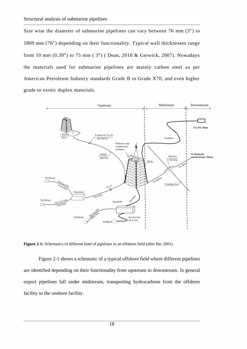
Size wise the diameter of submarine pipelines can vary between 76 mm (3) to
1800 mm (76) depending on their functionality. Typical wall thicknesses range
from 10 mm (0.39) to 75 mm ( 3) ( Dean, 2010 & Gerwick, 2007). Nowadays
the materials used for submarine pipelines are mainly carbon steel a s per
American Petroleum Industry standards Grade B to Grade X70, and even higher
grade to exotic duplex materials.
Figure 2-1: Schematics of different kind of pipelines in an offshore field (after Bai 2001).
Figure 2-1 shows a schematic of a typical offshore field where different pipelines
are identified depending on their functionality from upstream to downstream. In general
export pipelines fall under midstream, transporting hydrocarbons from the offshore
facility to the onshore facility.
To domestic market
Upstream Downstream
Wellhead
Service line
Flow lineWellhead
Wellhead
Manifold
Trunkline
To Domestic
market/Power Plants
Midstream
To LNG Plant
Platform with
compression
facilities
Structural analysis of submarine pipelines
19
2.2 STRUCTURAL ANALYSIS OF PIPELINES
Research and development on the structural analysis of submarine pipelines have
matured significantly over the last decade, due to the extensive use of pipelines in the
petroleum industry. The structural integrity of deepwater pipelines may be severely
challenged by extreme events, for example the geohazard of a submarine landslide (from
here on referred to as submarine slides) while crossing continental slopes from deepwater
towards the shore. Structural integrity issues also arise from the high temperature (HT)
and high pressure (HP) of the transported fluid, and the cyclic changes resulting from
operational shut down and start up cycles. Pipeline impact from a submarine slide causes
high bending and tensile stresses (and strains) in the pipe wall, leading to risk of fracture,
while HT/HP results in high compressive axial force in the pipe leading to buckling and,
as a result of shut down cycles, cumulative axial walking.
This chapter summarises current methods used to analyse the effects of submarine slides,
lateral buckling and walking mechanisms, and also relevant research on pipe-soil
interaction, which is a necessary prerequisite for analysing the pipeline system as a whole.
2.2.1 Submarine pipe-soil interaction
Published research on pipe-soil interaction may be classified into three major
categories - classical plasticity theory, finite element analysis and physical modelling
studies. McCarron (2011) summarised the design considerations for subsea flowlines
against lateral and upheaval buckling. Simple numerical modelling techniques of pipe-
soil interactions are also highlighted in the book. Randolph & Gourvenec (2011) also
presented the key aspects of offshore pipeline design and current practices in their chapter
‘pipeline and riser geotechnics’. Summaries of recent developments on pipe-soil
interrelations have been provided by Cathie et al. (2005) and White and Cathie (2010).

Structural analysis of submarine pipelines
20
Here, a brief overview of some of the analytical methods are given that have contributed
to design approaches.
The geotechnical design of deepwater pipelines resting on shallow sediment is
concerned primarily with the issues associated with lateral buckling, and walking. These
two issues have been the topic of a longstanding joint industry project, the SAFEBUCK
JIP (Bruton et al. 2006, 2008, Collberg et al. 2011). The axial and lateral resistances
offered by the shallow sediments are key inputs to the design and depend on the
embedment of the pipeline, and on the velocity and time of the movement relative to the
soil consolidation characteristics (Randolph, 2013).
Geotechnical aspects of the vertical response of on-bottom pipelines have been
researched extensively in the past two decades by various researchers. Plasticity solutions
may be used for simple static penetration (Randolph & White 2008b, Martin & White
2012). After laying of the pipeline it undergoes hydro testing before commencing
operations, where it will be subjected to cycles of high pressure and high temperatures.
The axial expansion of a pipeline due to thermal loading mobilises axial resistance similar
to that of shaft resistance on a vertically-loaded pile (Randolph & White, 2008a). Even
though at face value the axial resistance would seem to be trivial (a sliding failure with
known vertical load), it turns out to be more complex in practice due to sensitivity to the
curved surface of the pipe and also the degree of consolidation before and during axial
movement.
Merifield et al. (2008) considered the response of shallowly embedded pipelines
under vertical and horizontal load, comparing the limiting loads with those calculated
using upper bound plasticity, and proposing yield envelopes covering different
combinations of vertical and horizontal load. Pipeline penetration and response under
subsequent lateral movements requires relatively sophisticated large deformation

Structural analysis of submarine pipelines
21
approaches to simulate. Using an Arbitrary Lagrangian Eulerian (ALE) approach, Konuk
& Yu (2007) and Yu & Konuk (2007) studied the large displacement pipe-soil interaction
problem. Merifield et al. (2009) also studied the vertical penetration response of pipes
and subsequent horizontal resistance for pushed-in-place (PIP) pipes. Wang et al. (2010)
and Chatterjee et al. (2012) studied large amplitude lateral motion of a pipe using a RITSS
approach (Hu & Randolph, 1998), but implemented for the first time in finite element
software ABAQUS (see Figure 2-2). Such large deformation, two and three dimensional,
finite element analyses are relatively difficult to perform and as such are not economic
for design from a project schedule perspective. Martin et al. (2013) provided a more
economic approach to overcome this difficulty with widely-spaced 2D soil slices
connected to a 3D pipe model, but even that approach would be outside the capability of
most projects.
Figure 2-2: Large deformation finite element analysis of pipeline penetration into highly layered material
(Chatterjee et al. 2012).
Pipeline resistance during large amplitude lateral movements has been investigated
by physical modelling (White & Dingle 2011). Embedment of the pipeline occurs due to
the submerged weight of the pipe and during additional cyclic motions the lay process

Structural analysis of submarine pipelines
22
(Westgate et al., 2009, 2010). Cathie et al. (2005) summarised various models proposed
by Wagner et al. (1987), Lieng et al. (1988), Verley & Sotberg (1992) and Verley & Lund
(1995) used for assessing lateral resistance of partially embedded pipelines. Large and
small-scale tests were reported by Bruton et al. (2006) to provide the key parameters
affecting lateral pipe-soil interaction response in soft clay soils.
Much of the existing data on axial resistance is publicly available in international
journals, conference proceedings and technical notes, mostly linked with three major
pipeline design JIPs such as HotPipe ( Collberg et al. 2005), SMARTPIPE® (White et al
2010) and SAFEBUCK (Collberg et al. 2011) were completed over the last two decades.
Among them the SAFEBUCK JIP (Collberg et al. 2011) was completed most recently
and aimed at pipeline-seabed interaction specifically, and some of its work has been
completed at the University of Western Australia, as described by and White and
Randolph (2007) and White et al. (2017).
In the case of deepwater pipelines, the effects of hydrodynamic loading is relatively
small and the dominant forces are from high internal temperature and pressure, which
tend to expand the pipes, increasing the net axial force (Bruton et al., 2008). Axial
resistance between the pipe and the seabed opposes this expansion. Excessive
compressive forces lead to buckling, but the buckling response depends critically on the
lateral soil resistance. When buckling occurs, it significantly reduces the axial loading.
On the other hand, excessive buckling may lead to high bending strains in the pipe section.
So, a controlled buckling may be a feasible solution for relief of thermal loading. If the
soil resistance is too high, there will be an accumulation of axial loading in the pipe.
Cumulative axial movement due to repeated thermal cycles may lead to global
displacement of pipes. This phenomenon is called ‘walking’ (Carr et al., 2006). For
design purposes, it is very important to assess pipeline buckling and walking accurately.

Structural analysis of submarine pipelines
23
Recent design approaches to control buckling and walking have necessitated predicting
the soil forces on mobile pipelines (White & Cheuk, 2008), accounting for the associated
changes in seabed geometry and strength. The existing models are mainly derived for
stability analyses. There is a need to extend existing models to account for geometry
changes, remoulding and reconsolidation effects that influence large amplitude cyclic
displacements.
Axial Passive response:
It is increasingly recognised that in the axial direction, the pipe-soil ‘t-z’ interaction
response is highly sensitive to the rate of movement (which affects the drainage
conditions) and, for cyclic loading (from thermal events, for example), the pause period
between events is important (Randolph & White 2008). This means that a wide range of
axial friction factors ( typically ranging from 0.1 to unity), and corresponding maximum
load transfer forces, can apply in different conditions. There is still limited understanding
of how strongly and in what ways the adopted axial pipe-soil parameters affect the
resulting pipeline response under thermal loading.
The passive interaction of the seabed and the pipe has been studied by many groups
and there are many reports and publications available on this topic. A summary of current
research and practice in this area is given by publications related to SAFEBUCK JIP
(Collberg et al. 2011) and White et al. (2017). In conventional design approach the pipe
seabed interaction model is idealized by spring-slider systems distributed along the length
of the pipeline. The ultimate axial resistance per unit length, F, may be expressed in terms
of the submerged weight of the pipe, W, a friction coefficient, μ, and an enhancement
factor, ζ, to account for wedging around the curved surface of the pipe: (Randolph and
White 2008b).

Structural analysis of submarine pipelines
24
𝐹 = 𝜇𝑁 = 𝜇𝜁𝑊 (2.3)
This is a simple formula but resolving the parameters and is very challenging. An
alternative approach used to estimate the axial resistance is called the total stress (alpha)
method, and is comparable to the equivalent technique to estimate axial pipe capacity,
with the axial resistance per unit length expressed as:
𝐹 = 𝛼𝑠𝑢𝐷𝜃𝐷′ (2.4)
Here α is the friction ratio, i.e. ratio of unit interface shear resistance τf to the undrained
strength, su, of the adjacent soil around the pipe; θD' is the half contact angle between the
pipe (of diameter D) and the seabed, so that θD'D is the contact perimeter.
The resistance of the seabed depends on the embedment or w/D ratio. When the
pipe is embedded it undergoes cyclic large horizontal movement in zones where buckling
occurs, due to thermal expansion and contraction. The SAFEBUCK JIP (Collberg, et al.
2011) highlighted that the axial breakout response can show a significant peak. The peak
in resistance that can occur falls away to a residual axial friction after breakout. A
significant peak in axial resistance can occur when the pipe moves axially for the first
time, or may be after a period of rest during which consolidation occurs. The first
movement is associated with the buckle formation. The displacement associated with the
peak is termed as the ‘mobilization displacement’. This effect has parallels in the brittle
‘t-z’ response of piles.
This significant (or otherwise) of a peak in the axial response has been studied in
relation to pile capacity by Murff (1980) and Randolph (1983). They used load transfer
curves which strain-softened abruptly or progressively once the full shaft friction was
mobilized. However, the influence on the ultimate capacity of the pile of a brittle peak
and strain softening of the soil response reduces as the axial pile stiffness increases, due

Structural analysis of submarine pipelines
25
to progressive failure. Exactly the same effect is relevant to pipelines under axial loading,
for axial loading either from a slide or thermal expansion.
The advantages and limitations of the alpha (or total stress) and beta (or effective stress)
approaches are well documented elsewhere (White and Randolph 2007; Oliphant and
Maconochie 2007; Randolph and White 2008a; Jewell and Ballard 2011; White et al.,
2011; White and Cathie, 2010). A new framework was proposed by White et al. (2012)
based on the concept of critical state of soil mechanics to incorporate the undrained and
drained conditions at the pipe-soil interface. Four elements of the frameworks are shown
in Figure 2-3.
Figure 2-3: Mechanisms affecting axial pipe-soil interaction (White et al. 2012)
Elastic stiffnesses
Selection of elastic stiffness for pipe–soil interaction springs is covered
inconsistently in the literature, without a definitive set of rigorous coefficients to rely on.
For example, Tian et al. (2010) and Tian and Cassidy (2011) proposed taking horizontal
elastic stiffness as equal to vertical elastic stiffness in their advanced pipe–soil interaction
Structural analysis of submarine pipelines
26
model. Hodder and Cassidy (2010), in their plasticity model, considered the ratio of
horizontal elastic to vertical elastic stiffness to be 0.925, basing it on Gazetas et al. (1985)
and Gazetas and Tassoulas (1987) for strip footings on an elastic half-space. The DNV
(2006b) design code provides additional alternative recommendations.
Along with the vertical and lateral stiffnesses the pre-failure axial stiffness of the pipeline
is important as a boundary condition for analysis of pipeline walking or the feed-in to
lateral buckles or submarine slide impact. At an element level, the axial stiffness may be
estimated by assuming a simple distribution of shear stress around the perimeter of the
pile, similar to that for normal effective stress (Randolph, 2013). Where the shear
modulus of the soil increases proportionally with depth, the axial elastic pipe-soil stiffness
can be estimated by the product of the shear modulus gradient and the diameter of the
pipe.
2.2.2 Geohazard – submarine slides
Until the last decade very limited research was conducted on historic submarine
slide systems that lie in oil and gas development regions, such as the Storegga slide off
the coast of Norway (Bugge et al. 1998) and the margins of the Mississippi delta where
submarine mudslides have been triggered by major hurricanes (Gilbert et al. 2007). The
submarine slide hazards of Australia’s North West Shelf have been highlighted by
Hengesh et al. (2011, 2013), Zhang et al. (2015). The outcomes of a 3-year COFS-
MERIWA JIP funded by six operators on the impact of submarine slides on pipelines has
been presented by White et al. (2016).
Global perspective:
As the oil and gas industry is extended into deeper water, there is an increase in the
prevalence of geohazards near submarine pipelines. The pipelines cross a wide range of
geographical terrain and must eventually cross the continental shelf break. The most
Structural analysis of submarine pipelines
27
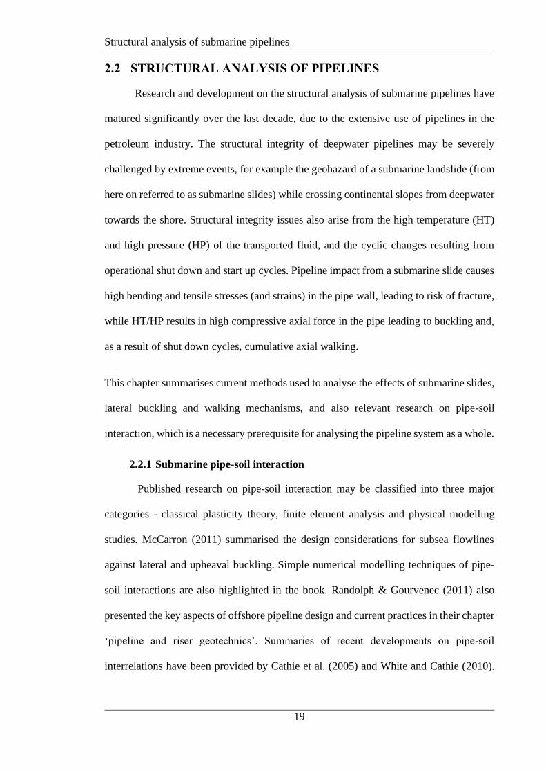
significant geohazard in this region is the potential for landslides. Therefore, the
development of reliable pipeline–slide models is essential. Jeanjean et al. (2005) have
given a perspective on some of the challenges faced by the oil and gas operators when
siting and designing their pipelines in landslide prone area of Gulf of Mexico (see Figure
2-4).
Figure 2-4: Seabed topography and field architectures of the Mad Dog field, Atlantis field, and Mardi
Gras Export transportation system in the Southern Green Canyon area of the Gulf of Mexico
(Jeanjean et al., 2005).
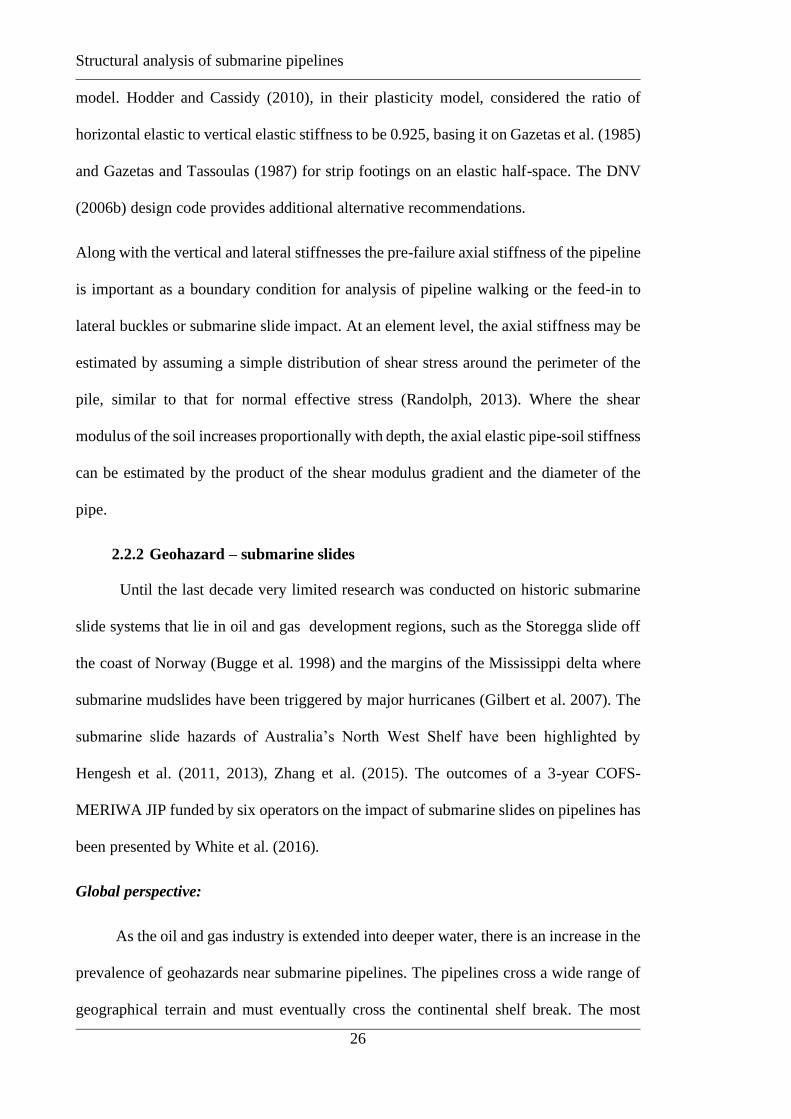
There is also a plan to construct a high pressure deepwater pipeline over 1300 km (Nash
& Roberts, 2011) of highly variable geologic conditions between the Middle East and
India across the Indus River fan as shown in Figure 2-5. The performance of offshore and
onshore buried and on-bottom pipelines subjected to ground surface rupture, soil
liquefaction, and other seismic hazards is critical for engineers to understand.
Structural analysis of submarine pipelines
28
Figure 2-5: Morpho-tectonic map of proposed Oman-India deepwater pipelines (Nash & Roberts, 2011)
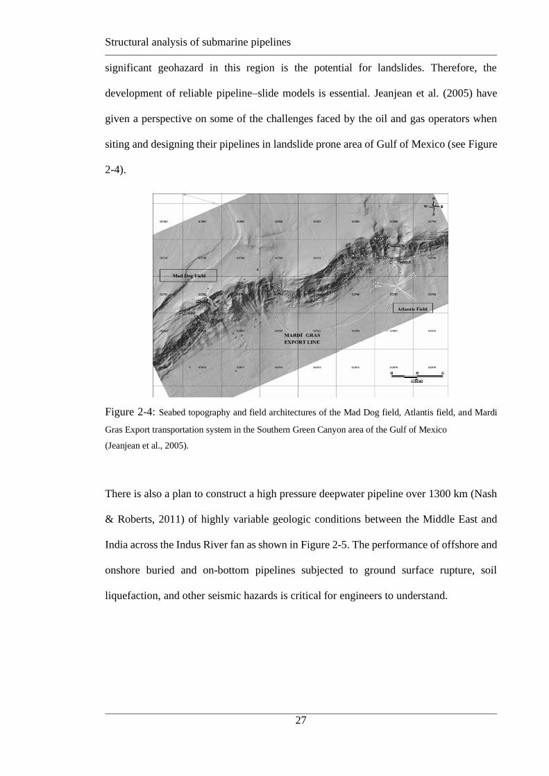
Seismic hazard analysis for the proposed Oman-India submarine pipeline was carried out
a few years ago (Campbell et al. 1996). The ground shaking hazard along the route of the
pipeline and in the Indus Canyon was found out to be relatively high. Due to this ground
shaking other potential geohazards such as liquefaction and triggering of submarine slides
may occur. Figure 2-6 shows the route of the pipeline and seismic activities in nearby
areas.
Figure 2-6: Seismic vulnerability of Oman-India deepwater pipeline (Campbell et al 1996)
Structural analysis of submarine pipelines
29
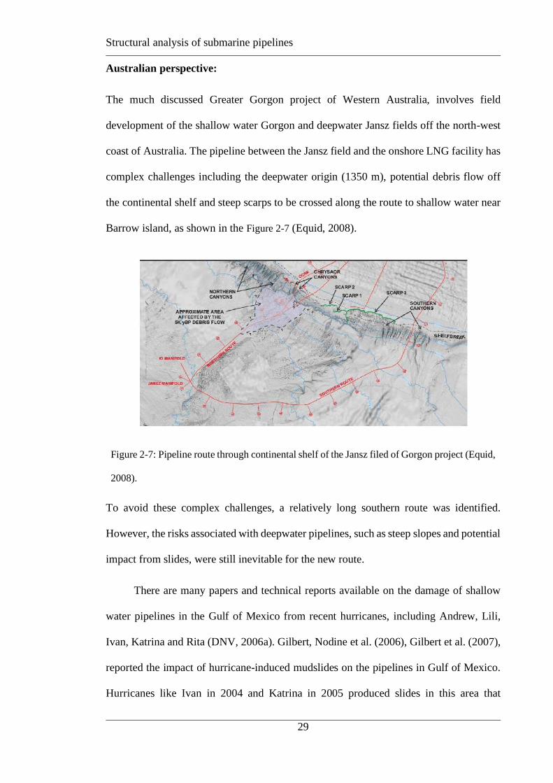
Australian perspective:
The much discussed Greater Gorgon project of Western Australia, involves field
development of the shallow water Gorgon and deepwater Jansz fields off the north-west
coast of Australia. The pipeline between the Jansz field and the onshore LNG facility has
complex challenges including the deepwater origin (1350 m), potential debris flow off
the continental shelf and steep scarps to be crossed along the route to shallow water near
Barrow island, as shown in the Figure 2-7 (Equid, 2008).
Figure 2-7: Pipeline route through continental shelf of the Jansz filed of Gorgon project (Equid,
2008).
To avoid these complex challenges, a relatively long southern route was identified.
However, the risks associated with deepwater pipelines, such as steep slopes and potential
impact from slides, were still inevitable for the new route.
There are many papers and technical reports available on the damage of shallow
water pipelines in the Gulf of Mexico from recent hurricanes, including Andrew, Lili,
Ivan, Katrina and Rita (DNV, 2006a). Gilbert, Nodine et al. (2006), Gilbert et al. (2007),
reported the impact of hurricane-induced mudslides on the pipelines in Gulf of Mexico.
Hurricanes like Ivan in 2004 and Katrina in 2005 produced slides in this area that
Structural analysis of submarine pipelines
30
damaged many pipelines (Mineral Management Services 2005).. These mudslides are
generally localized features of several thousands of feet (1-3 km) long by hundreds of
feet (30 – 300 m) across by 50 to 100 feet (15 – 30 m) deep. Damage to the pipelines in
the vicinity of the mudslide zone are due to excessive longitudinal forces (Randolph et
al., 2010). More reliable techniques of assessing the normal and axial impact forces
generated by mudslide loading, which result in high tensile longitudinal forces in the
pipeline, would aid the prediction and mitigation of hurricane damage. However, in
contrast to the understanding of the common mudslide events that affect the dense
network of shallow Gulf of Mexico pipelines, there are very few reports in the technical
literature on potential or actual geohazard damage to deepwater pipelines, which is partly
because deepwater pipelines are only recently being developed.
Structural response submarine pipelines impacted by submarine slide:
Sweeney et al. (2004) and Parker et al. (2008) presented a similar ‘string’ or ‘cable’
model of the submarine pipelines, where the pipe was assumed to resist tension but not
bending. In this model, the pipeline was subjected to uniform normal loading by the soil
inside the slide area and outside the slide area. Assuming that the normal force per unit
area is balanced in the two regions, from equilibrium, the normal force in the region
outside the slide occurs over a distance L/2 on each side, where L is the width of the slide.
It was shown from moment equilibrium that the ‘string’ deforms into a double parabola,
whose shape was defined as a function of applied load and tension at the centre of the
parabola. Both the models assume that the tension in the pipeline was uniform over a
central region, and that it decreased gradually to zero outside of this region, due to being
opposed by the axial soil resistance. Parker et al (2008) considered that the uniform
tension applies to the landslide region of width L, whereas Sweeney et al. (2004) applied

Structural analysis of submarine pipelines
31
the uniform tension to a region of length 2L (the entire region loaded laterally by the soil,
either actively or passively).
In a different mudslide loading model, Swanson & Jones et al. (1982) explicitly
accounted for the extra length (geometric slack) provided by laying the pipeline with
some curves. Their model was based on the equilibrium and compatibility equations for
an inextensible rod loaded axially and transversely allowing for the finite deflection. This
model was used to determine the maximum width of slide for different conditions by
changing the various parameters including pipe diameter, pipe thickness, pipe weight,
buried or surface laid and inclination of the slide with the pipe axis. The governing
equations were integrated in closed form between the characteristic nodes 1-4 as shown
in Figure 2-8.
Figure 2-8: Schematic of landslide impact on pipelines (Swanson &Jones et al. 1982)
The results showed that the burial of a pipeline outside the slide zone was safer because
active loading was reduced or eliminated and the passive support loading was increased.
It was also observed that with increasing inclination angle of the slide with the pipe axis,
the likelihood of failure reduced. Only downslope soil movement was considered in their
study.
Structural analysis of submarine pipelines
32
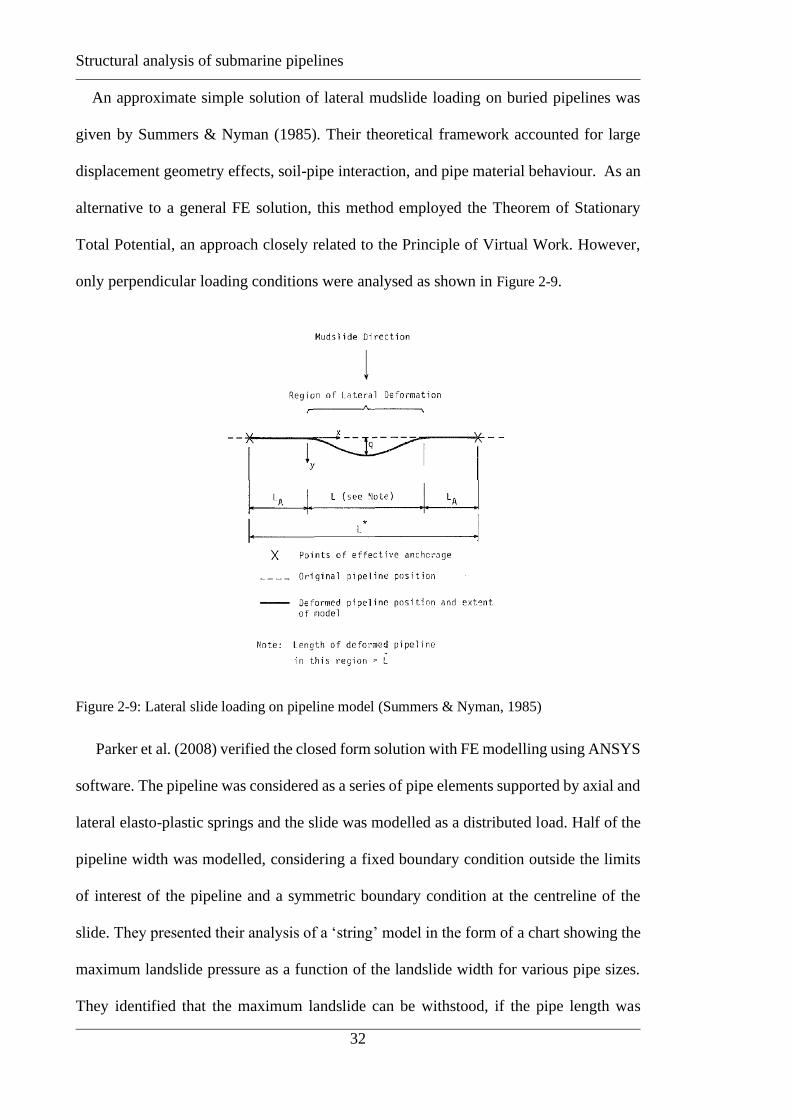
An approximate simple solution of lateral mudslide loading on buried pipelines was
given by Summers & Nyman (1985). Their theoretical framework accounted for large
displacement geometry effects, soil-pipe interaction, and pipe material behaviour. As an
alternative to a general FE solution, this method employed the Theorem of Stationary
Total Potential, an approach closely related to the Principle of Virtual Work. However,
only perpendicular loading conditions were analysed as shown in Figure 2-9.
Figure 2-9: Lateral slide loading on pipeline model (Summers & Nyman, 1985)
Parker et al. (2008) verified the closed form solution with FE modelling using ANSYS
software. The pipeline was considered as a series of pipe elements supported by axial and
lateral elasto-plastic springs and the slide was modelled as a distributed load. Half of the
pipeline width was modelled, considering a fixed boundary condition outside the limits
of interest of the pipeline and a symmetric boundary condition at the centreline of the
slide. They presented their analysis of a ‘string’ model in the form of a chart showing the
maximum landslide pressure as a function of the landslide width for various pipe sizes.
They identified that the maximum landslide can be withstood, if the pipe length was
Structural analysis of submarine pipelines
33
greater than the (passive) anchor length. They also noted that, if the PLET (pipeline end
termination) was less than the minimum anchor length then the pipe would slide before
yielding, thus reducing the maximum sustainable slide loading.
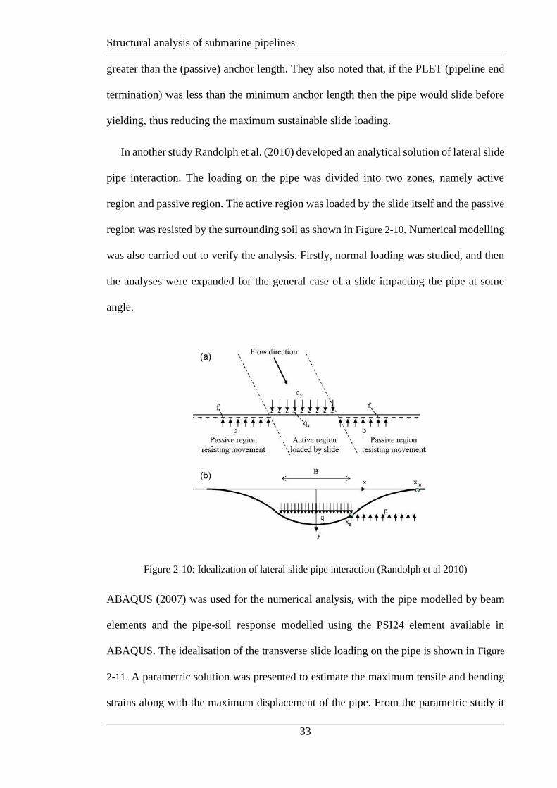
In another study Randolph et al. (2010) developed an analytical solution of lateral slide
pipe interaction. The loading on the pipe was divided into two zones, namely active
region and passive region. The active region was loaded by the slide itself and the passive
region was resisted by the surrounding soil as shown in Figure 2-10. Numerical modelling
was also carried out to verify the analysis. Firstly, normal loading was studied, and then
the analyses were expanded for the general case of a slide impacting the pipe at some
angle.
Figure 2-10: Idealization of lateral slide pipe interaction (Randolph et al 2010)
ABAQUS (2007) was used for the numerical analysis, with the pipe modelled by beam
elements and the pipe-soil response modelled using the PSI24 element available in
ABAQUS. The idealisation of the transverse slide loading on the pipe is shown in Figure
2-11. A parametric solution was presented to estimate the maximum tensile and bending
strains along with the maximum displacement of the pipe. From the parametric study it
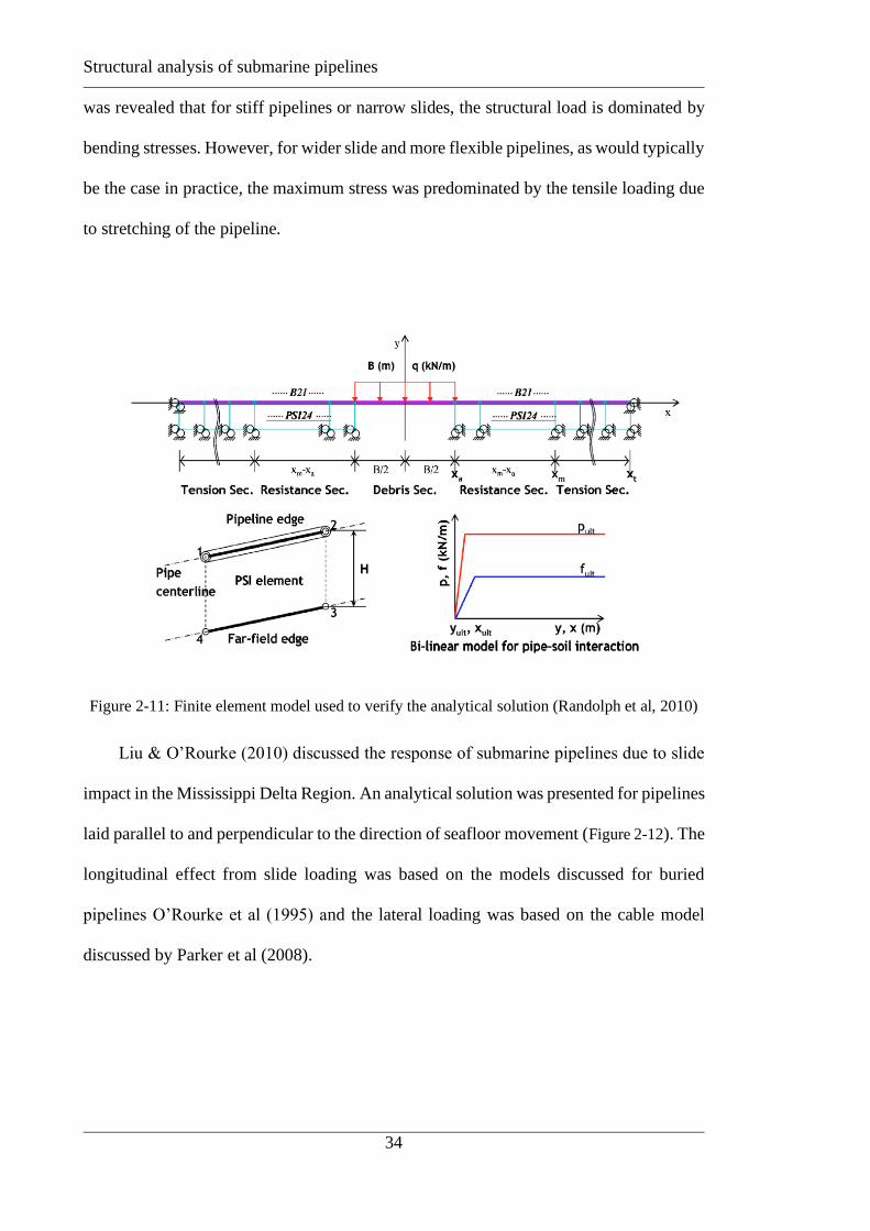
Structural analysis of submarine pipelines
34
was revealed that for stiff pipelines or narrow slides, the structural load is dominated by
bending stresses. However, for wider slide and more flexible pipelines, as would typically
be the case in practice, the maximum stress was predominated by the tensile loading due
to stretching of the pipeline.
Figure 2-11: Finite element model used to verify the analytical solution (Randolph et al, 2010)
Liu & O’Rourke (2010) discussed the response of submarine pipelines due to slide
impact in the Mississippi Delta Region. An analytical solution was presented for pipelines
laid parallel to and perpendicular to the direction of seafloor movement (Figure 2-12). The
longitudinal effect from slide loading was based on the models discussed for buried
pipelines O’Rourke et al (1995) and the lateral loading was based on the cable model
discussed by Parker et al (2008).
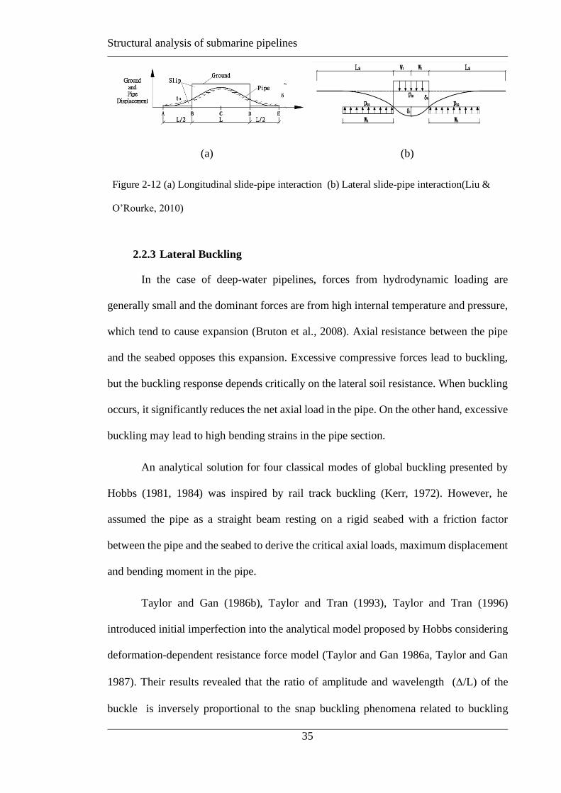
Structural analysis of submarine pipelines
35
(a)
(b)
Figure 2-12 (a) Longitudinal slide-pipe interaction (b) Lateral slide-pipe interaction(Liu &
O’Rourke, 2010)
2.2.3 Lateral Buckling
In the case of deep-water pipelines, forces from hydrodynamic loading are
generally small and the dominant forces are from high internal temperature and pressure,
which tend to cause expansion (Bruton et al., 2008). Axial resistance between the pipe
and the seabed opposes this expansion. Excessive compressive forces lead to buckling,
but the buckling response depends critically on the lateral soil resistance. When buckling
occurs, it significantly reduces the net axial load in the pipe. On the other hand, excessive
buckling may lead to high bending strains in the pipe section.
An analytical solution for four classical modes of global buckling presented by
Hobbs (1981, 1984) was inspired by rail track buckling (Kerr, 1972). However, he
assumed the pipe as a straight beam resting on a rigid seabed with a friction factor
between the pipe and the seabed to derive the critical axial loads, maximum displacement
and bending moment in the pipe.
Taylor and Gan (1986b), Taylor and Tran (1993), Taylor and Tran (1996)
introduced initial imperfection into the analytical model proposed by Hobbs considering
deformation-dependent resistance force model (Taylor and Gan 1986a, Taylor and Gan
1987). Their results revealed that the ratio of amplitude and wavelength (/L) of the
buckle is inversely proportional to the snap buckling phenomena related to buckling

Structural analysis of submarine pipelines
36
temperature and buckle deformation. Later Liu et al. (2014) extended the analytical
solution and provided the relationship between the critical buckling temperature,
buckling length and amplitude under different high-order global lateral buckling modes.
Hong et al ( 2015) compared results of analytical and finite element solutions for high
order lateral buckling modes with a single arch imperfection. Zhu et al. (2015)
investigated analytically the localised lateral buckling of a straight pipe
Beam buckling in the vertical mode and in the lateral mode was studied by Chi &
Chiou (1995). Elasto-plastic beam elements were used to model a pipe with nominally
infinite length and large local deformation. Their results revealed that the buckling
behaviour of a buried submarine pipeline is influenced by the burial depth and the initial
imperfection of the pipe. The lateral buckling load is greatly reduced for shallow burial,
larger initial imperfection.
Torselleti et al. (1999) in the Hotpipe project carried out FE analysis with
ABAQUS of a submarine pipeline resting on a flat seabed. They employed the RIKS
method to compare the analytical buckling solution with their numerical results for initial
imperfection and pipe material properties. They also carried out analyses to select the
best element for the pipeline. The pipe was modelled using a combination of pipe and
elbow elements to incorporate the advantages of both elements. Pipe elements were used
for the straight section and elbow elements were used for the buckle section. Nonlinear
seabed pipe interaction was modelled in the lateral and axial directions. A number of
analyses were carried out to compare the available analytical buckling solution with the
numerical results. In the end they concluded that initial imperfection and lateral soil-pipe
friction forces are very important in the development of the stress-strain behaviour of the
buckle.

Structural analysis of submarine pipelines
37
The effect of initial imperfection was also studied by Sriskandarajah et al (1999)
with FE analysis. They used an arc-length method to investigate lateral buckling
influenced by lay induced imperfections. However, they failed to explore the significance
of soil properties in the buckling analyses. A buckling solution with nonlinear pipe
material was given by Peek & Yun (2004 ). They gave a scaled solution of lateral buckling
using FE analysis. They incorporated the elastic-plastic behaviour of the pipe material
and the lateral soil resistance was modelled with a series of nonlinear elastic springs
attached to each pipe node. The mobilisation displacement for this lateral soil resistance
force was taken to be small enough not to affect the results, but large enough for
numerical stability. The pipe was modelled with the elastic-perfectly plastic beam
element available in ABAQUS.
Peek & Yun (2007) gave an analytical solution of lateral buckling triggered by flotation.
Then they used 3-D FE analysis carried out with ABAQUS to verify the analytical model.
The ABAQUS B31H element was used for the pipe and the seabed was modelled with
rigid elements. They found that from the FE analysis the bifurcation point occurred
slightly before the peak axial load. This leads to the conclusion that lateral instability
dominates the equilibrium position.
2.2.4 Pipeline Walking
Submarine pipelines are increasingly operating at high temperature and high pressure
(HP/HT) (Carr et al. 2003). Figure 2-13 shows the trend and development of submarine
pipelines continuously subjected to HP/HT regime. The pipelines operating at HP/HT
have a high tendency to Euler global buckling and walking. Recent projects have
developed better ways to control lateral buckling. However, challenges remain in
quantifying and mitigating the more complex issues associated with walking. Pipeline

Structural analysis of submarine pipelines
38
walking can be summarised simply as a phenomenon in which start-up/shut down cycles
cause a ratcheting response in the pipe lead to axial displacement (Carr et al 2003).
Figure 2-13: Trend of submarine pipelines being subjected to HP/HT (Carr et al 2003)
Palmer & Ling (1981) presented an analytical model for the pipeline expansion near
the platform, comparing the results with the two cases of North Sea pipelines. They
considered an elastic pipeline resting on a seabed that expands more towards the platform
and less away from the platform due to the fluctuating operating temperature and pressure.
The smaller expansion of the pipeline away from the platform was restrained by the
frictional resistance between the pipe and the seabed. When the operating temperature
and pressure are reduced, the movement of the pipeline reverses away from the platform.
The movement of the pipeline towards the platform was expressed separately for
exponential temperature increase with distance from the platform and also for uniform
temperature increase. When the temperature, θ1 is an exponential function of distance
from the platform, the expansion of the pipeline was expressed as:
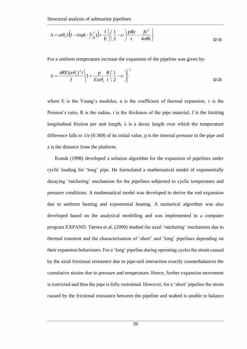
Structural analysis of submarine pipelines
39
( )
−
−+−−=
Rt
fz
t
pRz
Ez
42
11)exp(1
2
1
(2-1)
For a uniform temperature increase the expansion of the pipeline was given by:
2
1
2
1
2
11
)(
−+=
t
R
E
p
f
tRE
(2-2)
where E is the Young’s modulus, α is the coefficient of thermal expansion, ν is the
Poisson’s ratio, R is the radius, t is the thickness of the pipe material, f is the limiting
longitudinal friction per unit length, λ is a decay length over which the temperature
difference falls to 1/e (0.369) of its initial value, p is the internal pressure in the pipe and
z is the distance from the platform.
Konuk (1998) developed a solution algorithm for the expansion of pipelines under
cyclic loading for ‘long’ pipe. He formulated a mathematical model of exponentially
decaying ‘ratcheting’ mechanism for the pipelines subjected to cyclic temperature and
pressure conditions. A mathematical model was developed to derive the end expansion
due to uniform heating and exponential heating. A numerical algorithm was also
developed based on the analytical modelling and was implemented in a computer
program EXPAND. Tørnes et al. (2000) studied the axial ‘ratcheting’ mechanism due to
thermal transient and the characterisation of ‘short’ and ‘long’ pipelines depending on
their expansion behaviours. For a ‘long’ pipeline during operating cycles the strain caused
by the axial frictional resistance due to pipe-soil interaction exactly counterbalances the
cumulative strains due to pressure and temperature. Hence, further expansion movement
is restricted and thus the pipe is fully restrained. However, for a ‘short’ pipeline the strain
caused by the frictional resistance between the pipeline and seabed is unable to balance

Structural analysis of submarine pipelines
40
the cumulative strains due to pressure and temperature even with friction has been
mobilised along its length.
Perinet & Frazer (2006) illustrated the walking mechanism due to SCR tension. When
the pipes is subjected to SCR tension and undergoes a thermal cycle, the fixed point
during heat up and cool down steps differs and the pipe moves towards the SCR loading
at each cool down (resulting from a shutdown operation). The pipe expands in the
opposite direction from the fixed point with the expansion resisted by the soil resistance.
However, they did not provide an analytical solution for the behaviour of pipelines during
thermal cycles.
Carr et. al. (2006) gave expressions for the pipeline walking under various field
conditions, as part of the SAFEBUCK JIP. They noted that pipeline walking behaviour
of short pipelines occurs due to: 1) tension at each end of the pipeline, for example as
associated with a SCR; 2) global seabed slope along the length of the pipe; and 3) thermal
gradients along the pipeline during changes in operating conditions. The analytical
solution of pipeline walking per cycle, under the tension from an SCR was given by:
( )fEA
SLfSP RR
−+=
(2-3)
where ΔP is the change in fully constrained force, SR is the SCR tension, f is the axial
frictional force, L is the length of the pipeline and EA is the axial stiffness of the pipe.
Then the slope of the seabed (φ) was introduced in the above expression and the walking
per cycle was given by:
( ) ( )( ) ( )
−+=
EA
LLWLWP tancossin
(2-4)

Structural analysis of submarine pipelines
41
where, μ is the axial friction coefficient. The analytical model of walking due to thermal
transients was not straightforward and was solved by an incremental method. However,
a simple approximate solution for the distance walked per cycle was also given by:
−−
= 424
16
2
f
f
f
f
EA
Lf if f > fθ/6
(2-5)
EA
Lf
8
2= if f < fθ/6
(2-6)
where, fθ is the force generated by a thermal transient. The above expressions were
validated with FEA analysis. The effect of the mobilisation displacement for limiting
axial friction was also studied in the paper. The results of the FEA analysis showed that
walking displacement was reduced as the axial mobilisation displacement increases.
However, they mentioned that FEA analysis indicated that the mobilisation displacement
can prove critical in quantifying the walking behaviour of submarine pipelines.
Throughout the paper the axial frictional resistance was considered to be a fixed value.
Rong et al. (2009) evaluated the axial walking behaviour of deepwater flowlines
along with the mitigation strategies. Detailed numerical analyses were carried out with
ABAQUS. In their analyses the nonlinearity of pipe-soil parameters, material of the pipe,
seabed profile, pressure and temperature profile and the connected PLET (pipeline end
termination) resistance were all considered. The pipe was modelled with 3D pipe element
(PIPE31H) and the seabed was modelled with a 3D rigid surface. Axial and lateral friction
factors were used with peak and residual values based on Carr et. al. (2006).
Quasi-static analysis was performed as this was considered reasonable for axial
walking. A detailed sensitivity study was performed to investigate the effects of friction
factor, axial mobilisation distance, PLET and any other in-line structural resistances.
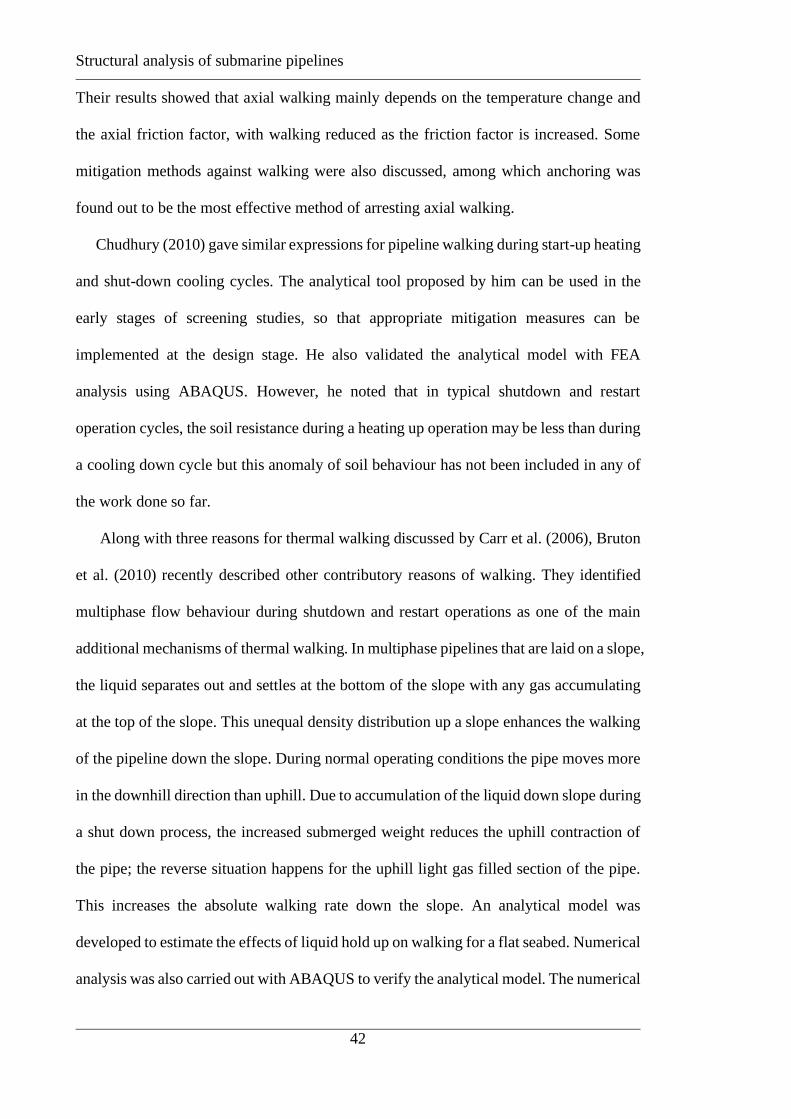
Structural analysis of submarine pipelines
42
Their results showed that axial walking mainly depends on the temperature change and
the axial friction factor, with walking reduced as the friction factor is increased. Some
mitigation methods against walking were also discussed, among which anchoring was
found out to be the most effective method of arresting axial walking.
Chudhury (2010) gave similar expressions for pipeline walking during start-up heating
and shut-down cooling cycles. The analytical tool proposed by him can be used in the
early stages of screening studies, so that appropriate mitigation measures can be
implemented at the design stage. He also validated the analytical model with FEA
analysis using ABAQUS. However, he noted that in typical shutdown and restart
operation cycles, the soil resistance during a heating up operation may be less than during
a cooling down cycle but this anomaly of soil behaviour has not been included in any of
the work done so far.
Along with three reasons for thermal walking discussed by Carr et al. (2006), Bruton
et al. (2010) recently described other contributory reasons of walking. They identified
multiphase flow behaviour during shutdown and restart operations as one of the main
additional mechanisms of thermal walking. In multiphase pipelines that are laid on a slope,
the liquid separates out and settles at the bottom of the slope with any gas accumulating
at the top of the slope. This unequal density distribution up a slope enhances the walking
of the pipeline down the slope. During normal operating conditions the pipe moves more
in the downhill direction than uphill. Due to accumulation of the liquid down slope during
a shut down process, the increased submerged weight reduces the uphill contraction of
the pipe; the reverse situation happens for the uphill light gas filled section of the pipe.
This increases the absolute walking rate down the slope. An analytical model was
developed to estimate the effects of liquid hold up on walking for a flat seabed. Numerical
analysis was also carried out with ABAQUS to verify the analytical model. The numerical
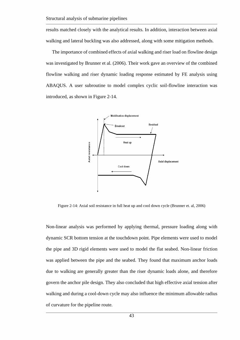
Structural analysis of submarine pipelines
43
results matched closely with the analytical results. In addition, interaction between axial
walking and lateral buckling was also addressed, along with some mitigation methods.
The importance of combined effects of axial walking and riser load on flowline design
was investigated by Brunner et al. (2006). Their work gave an overview of the combined
flowline walking and riser dynamic loading response estimated by FE analysis using
ABAQUS. A user subroutine to model complex cyclic soil-flowline interaction was
introduced, as shown in Figure 2-14.
Figure 2-14: Axial soil resistance in full heat up and cool down cycle (Brunner et. al, 2006)
Non-linear analysis was performed by applying thermal, pressure loading along with
dynamic SCR bottom tension at the touchdown point. Pipe elements were used to model
the pipe and 3D rigid elements were used to model the flat seabed. Non-linear friction
was applied between the pipe and the seabed. They found that maximum anchor loads
due to walking are generally greater than the riser dynamic loads alone, and therefore
govern the anchor pile design. They also concluded that high effective axial tension after
walking and during a cool-down cycle may also influence the minimum allowable radius
of curvature for the pipeline route.

Structural analysis of submarine pipelines
44
Flowlines may be seated on undulating slopes and with cyclic thermal gradients
during operation and shut down operations. Generally global movement is associated
with short or non-cyclically constrained pipelines, which move towards the cold end or
down the slope of the seabed. Wang et al. (2010) presented an analytical model for long
and partially constrained pipelines that can move towards either end when subjected to
cyclic loading. This analytical model captures a new ‘caterpillar-type’ of global
movement of the pipelines,. This migration of long pipelines depends on the localisation
of the transient pressure and temperature profile. The bi-linear axial friction was modelled
as shown in Figure 2-15.
Figure 2-15: Typical axial friction profile considered by Wang et al. (2010)
For the analytical modelling they divided the whole length of the pipelines into a stick-
slide zone is shown in Figure 2-16.

Structural analysis of submarine pipelines
45
Figure 2-16: Stick-slide model considered by Wang et al (2010)
They considered a different thermal profile for heating and cool down cycles for the stick-
slide model. The end displacement of the pipe after one cycle was plotted in Figure 2-17.
Figure 2-17: Movement of the pipe after 1st cycle with stick-slide model
The effect of friction mobilisation was studied over 40 cycles. They also noted the
importance of reviewing the simple pipe-soil interaction model adopted.
Axial pipe-soil interaction during walking
The present practice of assessing axial pipe-soil interaction was discussed in detail
earlier. In this section the available literature about pipe-soil interaction during walking
Structural analysis of submarine pipelines
46
is discussed in more detail. Advances in the study of soil-pipe interaction forces have
been described by many researchers (Cathie et al. 2005, White & Randolph 2007, and
White & Cathie 2010).
Hill & Jacob (2008) identified knowledge gaps and resulting assumptions in the
modelling the soil behaviour in many of the previous studies. They noted that, as the
pipeline is heated from one end to the other, it moves axially relative to the soil with
variable speeds at different positions along the route of the pipeline. This range might
typically vary from 0.0002 mm/s to a maximum of approximately 0.7 mm/s. To address
the gap in the literature and available methods, they developed an in-situ testing system
consisting of an instrumented pipe section suspended beneath a frame by means of a
hydraulic system. The axial, vertical and lateral movement of the pipe section, and
corresponding forces, were measured by transducers. The aim of the development was to
assess the functionality of shallowly embedded pipeline systems, acquiring and
interpreting the data from a geotechnical perspective and understanding the consolidation
characteristics of the soil and the pore pressure response during pipe movement in detail.
The equipment was projected to save significant CAPEX for a project by testing in situ,
thus saving time in transport bulk soil to the onshore laboratories.
Generally axial pipe soil interaction is modelled with a simple friction coefficient
that links the available ultimate resistance to axial movement to the weight of the pipe.
However, the response may not be completely frictional and changes in pipe weight may
not completely correspond to the corresponding changes in axial resistance (Bruton et. al.
2008). A finite displacement must occur at very small loads to reach the ultimate
resistance. Due to this finite mobilisation displacement, the initiation of buckling and
pipeline walking occurs at very small loads.

Structural analysis of submarine pipelines
47
Figure 2-18: Axial soil pipe interaction schematics with ultimate resistance and mobilisation displacement
(Bruton et al. 2008)
Figure 2-18 illustrates ductile, brittle and drained axial responses for pipelines, as
developed from laboratory testing. The brittle response consists of high breakout axial
resistance followed by a lower residual resistance. The breakout axial resistance can be
defined as the mobilisation of maximum friction at very small displacements. This
response is influenced by excess pore pressure generated at the pipe-soil invert. The very
small displacement at which the peak axial resistance occurs is referred to as the
mobilisation displacement and often called ‘elastic-slip’. The mobilisation displacement
depends on the soil conditions, pipe roughness and pipe embedment.
Once the pipe starts moving, for example during a thermal increase, the friction
reduces to a residual value at a larger displacements. The residual friction dominates the
end expansion of the pipe and the feed-in into a lateral buckle. If the pipe displacement
occurs very slowly and no excess pore pressure is generated, the response may be termed
‘drained’ (Bruton et al 2008). Carneiro & Murphy (2011) observed the effect of soil
mobilisation on the walking rate of pipeline numerically. The analytical solution
provided by Carr et al. (2006) is in good agreement with the FE results provided by White
et al. (2015). The difference between the results is due to the axial displacement, Xmob,
required to mobilize the full axial resistance in the FE analysis. Therefore, White et al.

Structural analysis of submarine pipelines
48
(2015) proposed an elastic correction of 2Xmob, subtracted from the predicted walk per
cycle, although without any mathematical justification. Therefore, an analytical model is
required to validate this elastic correction.
Pipeline walking and velocity dependent friction
Walking rates depend on the restraint associated with seabed friction. In
conventional analyses, seabed friction is independent of the rate of thermal loading and
expansion, although it has been recognised that the sliding resistance between a pipe and
the seabed varies with velocity, partly due to drainage effects. In conventional design
approaches, the rate of thermal loading during operating cycles is not considered within
the analysis. However, the velocity varies with position along the pipeline and with time
during each startup or shutdown event. Recently, it has been recognised that the sliding
resistance between a pipe and the seabed varies significantly with velocity due to drainage
effects (White et al. 2011, White & Cathie 2010), but to date much less research has been
done to incorporate this complex model (Carneiro et al. (2017) in any structural modelling
of pipeline walking to estimate equivalent friction factors.
2.3 CONCLUSIONS
To highlight the status of existing literature a brief discussion was presented in
this chapter to lay the foundation of this thesis. A short discussion is presented here to
highlight the gap in the existing literature and need of research.
Numerical simulations to derive the elastic t-z stiffness of a pipe resting on the
seafloor are overly complex and a simple solution is needed. Limited prior information
exists for the axial elastic response of on-bottom pipelines in the literature, particularly
for non-homogeneous soil. Therefore, an approximate analytical approach is needed for

Structural analysis of submarine pipelines
49
the axial stiffness, focusing on the most relevant case for deepwater pipelines of shear
modulus proportional to depth.
Geohazard assessment, and in particular quantifying the response of pipelines to
impact from submarine debris flow, has become a critical issue for the offshore pipeline
industry. The numerical modelling of the pipe structural response is also onerous –
particularly in a probabilistic world where designers want to run a million cases of
varying slide loading, strength, impact velocity etc. which means that an analytical
solution for the structural response of a straight pipe impacted by axial slide loading is
needed.
As discussed previously, deepwater pipelines are often subjected to operational
cycles of high temperature and high pressure. This rises the possibilities of lateral
buckling and or pipeline walking issues. Classical theories to predict the critical buckling
loads are simple and easy to use without any complexity of the soil-pipe interaction.
However, in practice the geotechnical parameters play a role, along with the as laid
geometry and pipe material. Therefore, a simple correlation (including all the relevant
parameters that influence lateral buckling) is needed in a generic non-dimensionalised
design chart to estimate the buckling load, valid for the range of inputs covered by the
parametric study.
Understanding the incremental walking mechanism of on bottom pipeline is
becoming challenging with the increasing complexities related to soil-pipe interaction on
soft clays, particularly when considering detailed aspects of pipe-soil interaction
behaviour. Therefore, to investigate the effects of complexities, such as elasto-plastic
soil behaviour and velocity dependent soil friction, simple analytical solutions supported
by numerical analyses need to be developed.

Structural analysis of submarine pipelines
50
In the concept stage of any submarine pipeline project, analytical solutions can
highlight the parameters that are most important when carrying out site investigation.
However, to validate final results of analytical solutions fine tuning of the design
generally requires numerical modelling, potentially supplemented by physical modelling.
In the following chapters axial pipe-soil interaction and structural analysis of submarine
pipe are presented, starting with analytical solutions followed by numerical modelling.

Structural analysis of submarine pipelines
51
References
Bai, Y. & Bai, Q. (2005). Subsea Pipelines and Risers. Elsevier Ltd.
Brunner, M. S., Qi, X., Zheng, J., & Chao, J. C. (2006) . Combined effect of flowline
walking and riser dynamic load on HP/HT flowline design. Proc. of Offshore
Technology Conference, Houston, USA, Paper OTC 17806.
Bruton, D., Sinclair, F., & Carr, M. (2010) . Lessons learned from observed walking of
pipelines with lateral buckles, including new driving mechanisms and updated
analysis models. Proc. of Offshore Technology Conference, Houston, USA, OTC
Paper 20750
Bruton D. A. S., White D. J., Cheuk C. Y., Bolton M. D. & Carr M. C. (2006). Pipe-soil
interaction behaviour during lateral buckling, including large amplitude cyclic
displacement tests by the Safebuck JIP. Proc. Offshore Technology Conf., Houston,
Paper OTC 17944.
Bruton, D. A. S, White, D. J., Carr, M. & Cheuk, C. Y. (2008). Pipe-soil interaction
during lateral buckling and pipeline walking – the Safebuck JIP. Proc. of Offshore
Technology Conference, Houston, Paper OTC 19589.
Bugge, T., Belderson, R.H. and Kenyon, N.H. (1998). The Storrega slide. Phil. Trans.
Royal Soc. of London 325, 357-388.
Campbell, K.W., Thenhaus, P.C. Mullee, J.E. & Preston, R. (1996). Seismic hazard
evaluation of the Oman India pipeline. Proc. of Offshore Technology Conference,
Houston, Paper OTC 8135.
Carneiro, D. & Murphy, D. (2011). Simple numerical models for pipeline walking
accounting for mitigation and complex soil response. Pro. of the ASME 2011 30th
Int. Conf. on Ocean, Offshore and Arctic Engineering OMAE2011.The
Netherlands. OMAE2011-49780.

Structural analysis of submarine pipelines
52
Carneiro, D., Rathbone, A., Siong, Soon, Kok., & Viecelli, G. (2017). Velocity-
Dependent Soil Resistance in Finite Element Analysis of Pipeline Walking.
Journal of Offshore Mechanics and Arctic Engineering. 139. 021701-1 .
10.1115/1.4034695.
Carr, M., Sinclair F, & Bruton D.(2006). Pipeline walking — understanding the field
layout challenges, and analytical solutions developed for the SAFEBUCK JIP.
Proc. Offshore Technology Conf., Houston, Paper OTC 17945.
Cathie D. N., Jaeck C, Ballard J. C. & Wintgens J-F. (2005). Pipeline geotechnics – state-
of-the-art. Proc. Int. Symp. On Frontiers in Offshore Geotechnics, Perth, 95-114
Chatterjee, S., White, D.J. and Randolph, M.F. (2012). Numerical simulations of pipe-
soil interaction during large lateral movements on clay. Géotechnique 62(8), 693–
705.
Chi, S. Y., & Chiou, Y. J. (1995). Buckling of offshore pipelines. Proc. 5th Int. Offshore
and Polar Engng Conf., Hauge, Netherlands, 95-107.
Collberg, Leif & Mo̸rk, Kim & Levold, Erik & Vitali, Luigino. (2005). HotPipe JIP:
Design Guidelines for HP/HT Pipelines. 683-690. 10.1115/OMAE2005-67523.
Collberg, L., Carr, M. and Levold, E. (2011). Safebuck Design Guideline and DNV-RP-
F110. Proceedings of the Offshore Technology Conference. OTC21575, Houston,
USA. DOI: 10.4043/21575-MS.
Dassault Systèmes (2007). ABAQUS analysis users’ manual, Simula Corp, Providence,
RI, USA.
Dean E.T.R. (2010). Offshore Geotechnical Engineering - Principles and Practice,
Thomas Telford, Reston, VA, U.S.A., 520 p.
DNV. (2006a). Technical Report, Pipeline damage assessment from Hurricane Ivan in
Structural analysis of submarine pipelines
53
Gulf of Mexico. Report No. 440 38570, Rev. 2.
DNV. (2006b). Free spanning pipelines. Recommend practice RP-F105, Det Norske
Veritas, Oslo, Norway.
DNVGL-RP-F114, DNV Recommended Practice F114. Pipe-soil interaction for
submarine pipelines. (2019) Det Norske Veritas, Norway Sept 2019.
Equid, D. (2008). Challenges of the Jansz deepwater tie-back: Gorgon Project. In
Conference CD of Deep Offshore Technology, Perth, Australia.
Gazetas, G., Dobry, R., and Tassoulas, J. L. (1985). Vertical response of arbitrarily
shaped embedded foundations. J. Geotech. Eng., 10.1061/ (ASCE)0733-
9410(1985)111:6(750), 750–771.
Gazetas, G., and Tassoulas, J. L. (1987). Horizontal stiffness of arbitrary shaped
embedded foundations. J. Geotech. Eng., 10.1061/(ASCE) 0733-
9410(1987)113:5(440), 440–457.
Gerwick B.C. (2007) Construction of marine and offshore structures. CRC Press, New
York, 795 p.
Gilbert R.B., Nodine, M.C., Wright, S.G., Cheon, J.Y., Wrzyszczynski, M., Coyne, M.
and Ward, E.G. (2007). Impact of hurricane-induced mudslides on pipelines. Proc.
Offshore Technology Conference, Houston, Paper OTC 18983.
Hengesh, J., Whitney, B., Rovere, A. (2011) A Tectonic Influence on Seafloor Stability
along Australia’s North West Shelf. Int. Offshore and Polar Engineering
Conference (ISOPE), USA, II, pp. 596-604.
Hengesh, J., Dirstein, J.K., Stanley, A.J. (2013) Landslide geomorphology along the
Exmouth plateau continental margin, North West Shelf, Australia. Australian
Geomechanics J., 48(4):71-92.
Structural analysis of submarine pipelines
54
Hill, A. J., & Jacob, H. (2008). In-situ measurement of pipe-soil interaction in deepwater.
Proc. of Offshore Technology Conference, Houston, USA, OTC 19528.
Hobbs, R. E. (1981). Pipeline buckling caused by axial loads. J. Construct. Steel Res.
1(2), 2-10.
Hobbs, R. E. (1984). In-service buckling of heated pipelines. J. Transport Eng., 110(2),
175-189.
Hodder,M. S., and Cassidy,M. J. (2010). A plasticity model for predicting the vertical
and lateral behaviour of pipelines in clay soils. Géotechnique, 60(4), 247–263.
Hong, Z., Liu, R., Liu, W., & Yan, S. (2015). Study on lateral buckling characteristics of
a submarine pipeline with a single arch symmetric initial imperfection. Ocean
Eng., 108, 21-32.
Hu, Y., & Randolph, M. (1998). H-adaptive FE analysis of elasto-plastic non-
homogeneous soil with large deformation. Computers and Geotechnics, 23(1/2),
61-83. https://doi.org/10.1016/S0266-352X(98)00012-3
Jeanjean, P., Hampson, K., Evans, T., Liedtke, E., and Clukey, E.C. (2005). An operator’s
perspective on offshore risk assessment and geotechnical design in geohazard-
prone areas. Proc, 2nd Int. Symp. Frontiers in Offshore Geotechnics, ISFOG 2010,
Perth, 115-143.
Jewell, R.J. & Ballard, J-C. (2011). Axial pipe-soil interaction – a suggested framework..
Proc. Offshore Tech. Conf., Houston, USA. Paper OTC 22010.
Kerr, A.D. (1972). On the stability of the railroad track in the vertical plane (No. NYU-
AA-72-35)
Konuk, I. (1998). Expansion of pipelines under cyclic operational conditions:
Formulation of problem and development of solution algorithm. Proc of 17th

Structural analysis of submarine pipelines
55
International Conference on Offshore Mechanics and Arctic Engineering.
OMAE98-1103
Konuk, I. & Yu, S. (2007). Continuum FE modelling of lateral buckling: study of soil
effects. Proc. of 26th Int. Conf. on Offshore Mechanics and Arctic Eng., San Diego,
OMAE2007-29376.
Lieng, J.T., Sotberg, T. & Brennodden, H. (1988). Energybased pipe-soil interaction
models. SINTEF Report to the American Gas Association.
Liu, R., Liu, W.B., Wu, X.L., & Yan, S.W. (2014). Global lateral buckling analysis of
idealized subsea pipelines. J. Cent. South Univ., 21, 416-427
Liu, J. & O'Rourke, M. (2010), Response of Offshore Pipelines to Landslides, Proc.
Offshore Technology Conf., Houston, Paper OTC 20525
Martin, C.M., Kong, D. & Byrne, B.W. (2013). 3D analysis of transverse pipe-soil
interaction using 2D soil slices. Géotechnique Letters 3: 119-123.
Martin, C.M. and White, D.J. (2012). Limit analysis of the undrained bearing capacity of
offshore pipelines. Géotechnique 62(9), 847-863.
McCarron, W. O. (2011). Deepwater foundations and pipeline geomechanics. J. Ross
publishing, Fort Lauderdale, USA.
Merifield, R. S., White, D. J. & Randolph, M. F. (2008). The ultimate undrained
resistance of partially embedded pipelines. Géotechnique 58, No. 6, 461-470.
Merifield R. S., White, D. J. & Randolph, M. F. (2009). Effect of surface heave on
response of partially embedded pipelines on clay. J. Geotech. Geoenviron. Engng,
ASCE 135, No. 6, 819-829.
Mineral Management Services (2005). Lists of pipelines damaged in hurricanes by lease
block, MMS Gulf of Mexico Region.
Structural analysis of submarine pipelines
56
Murff, J. D., Wagner, D. A. & Randolph, M. F. (1989). Pipe penetration in cohesive soil.
Géotechnique 39, No. 2, 213-229.
Nash, I., & Roberts, P. M. (2011). The deepwater gas route to India. Proc. 34th Annual
Offshore Pipeline Technology Conference, Amsterdam, UK.
Nodine, Mary C., Wright, Stephen G., Gilbert, Robert B. and Ward, E.G. (2006).
Mudflow and mudslide during Hurricane Ivan. Proc. Offshore Technology Conf.,
Houston, OTC 18328.
Oliphant, J. & Maconochie, A. (2007). The axial resistance of buried and unburied
pipelines. Proc. 6th Int. Conf. Offshore Site Investigation and Geotechnics.
London: Society for Underwater Technology, 125–132.
O’Rourke, M.J., Liu, X.J., and Flores-Berrones, R.,(1995). Steel pipe wrinkling due to
longitudinal permanent ground deformations. Journal of Transportation
Engineering, September/October, Vol. 121, No. 5, pp. 443-451.
Palmer, A.C., & Ling, M. T.S. (1981) Movement of submarine pipelines close to
platforms. Proc. 13th Offshore Technology Conf., Houston, Paper OTC 4067.
Parker, E., Traverso, C., Moore. R., Evans, T., Usher, N. (2008). Evaluation of landslide
impact on deepwater submarine pipelines. Proc. Offshore Technology Conf.,
Houston, Paper OTC 19459.
Peek, R. & Yun, H. (2004). Scaling of solutions for the lateral buckling of elastic plastic
pipelines, 23rd Int. Conf. on Offshore Mechanics and Arctic Engineering, Vol. 3,
Vancouver, British Columbia, Canada. OMAE2004-51054, 1-8
Peek, R. & Yun, H. (2007). Floation to trigger lateral buckles in pipelines on a flat seabed.
J. Eng. Mech. 133 (4), 442-451.
Perinet, D. & Frazer, I. (2006). Mitigation Methods for Deepwater Pipeline Instability
Induced by Pressure and Temperature Variations. Proc. Offshore Technology
Conference, Houston, Paper OTC 17815-MS.
Randolph, M.F. (1983). Design considerations for offshore piles. Proc. Conf. on Geot.
Practice in Offshore Engng, ASCE, Austin, 422-439.
Randolph, M.F. (2013). Analytical contribution to offshore geotechnical engineering.
Proc., 18th Int. Conf. on Soil Mechanics and Geotechnical Engineering,
Structural analysis of submarine pipelines
57
International Society of Soil Mechanics and Foundation Engineering ( ISSMFE),
85-105.
Randolph, M. F., Seo, D., & White, D. J. (2010). Parametric solution of slide impact on
pipelines. Journal of Geotech and Geoenvironmental Engineering, ASCE, July,
136(7), 940-949.
Randolph, M. & Gourvenec, S. (2011). Offshore geotechnical engineering. Spon Press,
Taylor & Francis Group, New York.
Randolph, M. F. & White, D. J. (2008a). Offshore Foundation Design – A Moving Target.
Proc. BGA International Conference on Foundations, Dundee, IHS BRE Press,
London, 27-59.
Randolph, M. F. & White, D. J. (2008b). Pipeline embedment in deepwater: process and
quantitative assessment. Proc. Offshore Technology Conference, Houston, Paper
OTC 19128.
Rong, H., Inglis, R., Bell, G., Huang, Z., & Chan, R. (2009). Evaluation and mitigation
of axial walking with a focus on deepwater flowlines. Proc. of Offshore Technology
Conference, Houston, USA, OTC 19862.
Sriskandarajah, T., Dong, S., S. Sribalachandran, S., & Wilkins, R. (1999). Effect of
initial imperfection on the lateral buckling of Subsea pipelines. Proc. 9th International
Offshore and Polar Engineering Conference, Brest, France, 168-175.
Summers, P. B., & Nyman, D. J. (1985). An approximate proceduce for assessing the
effects of mudslides on offshore pipelines. Offshore Mechanics & Arctic
Engineering Division, Transaction of ASME, Vol. 107. December, 426-432.
Swanson, R. C., and Jones, W. T. (1982). Mudslide effects on offshore pipelines.
Transportation Engineering Journal, ASCE, 108(TE6), 585-600.
Sweeney, M., Gasca, A. H., Garcia Lopez, M., and Palmer, A. C. (2004). Pipelines and
landslide in rugged terrain: A database, historic risk and pipeline vulnerability.
Proc. Int. Conf. on Terrain and Geohazard Challenges Facing Oil and Gas
Structural analysis of submarine pipelines
58
Pipelines, Thomas Telford, London, 647-659.
Taylor, N., Gan, A.B., 1986a. Refined modelling for the lateral buckling of submarine
pipelines. J. of Constr. Steel Res. 6 (2), 143–162.
Taylor, N., Gan, A.B., 1986b. Submarine pipeline buckling-imperfection studies. Thin-
Walled Struct. 4 (4), 295–323.
Taylor, N., Gan, A.B., 1987. Refined modelling for the vertical buckling of submarine
pipelines. J. of Constr. Steel Res. 7 (1), 55–74.
Taylor, N., Tran, V., 1993. Prop-imperfection subsea pipeline buckling. Mar. Struct. 6
(4), 325–358.
Taylor, N., Tran, V., 1996. Experimental and theoretical studies in subsea pipeline
buckling. Mar. Struct. 9 (2), 211–257.
Tian, Y., and Cassidy, M. J. (2011). Pipe-soil interaction model incorporating large lateral
displacements in calcareous sand.J. Geotech. Geoenviron. Eng., 137(3), 279–287.
Tian, Y., Cassidy, M. J., and Gaudin, C. (2010). Advancing pipe-soil interaction models
through geotechnical centrifuge testing in calcareous sand. Appl. Ocean Res., 32(3),
284–297.
Torselleti, E., Vitali, L., & Levold, E. (1999). Hotpipe Project: Snaking of submarine
pipelines resting on flat sea bottom using finite element method. Proc. 9th Int.
Offshore and Polar Engng. Conf., Brest, France, 34-45
Verley, R. L. P. & Lund, K. M. (1995). A soil resistance model for pipelines placed on
clay soils. Proc. Offshore Mechanics and Arctic Engineering Conf, Copenhagen,
18–22, Vol V: 225–232.

Structural analysis of submarine pipelines
59
Verley, R. L. P. & Sotberg, T. (1992). A soil resistance model for pipelines placed on
sandy soils. Proc. Offshore Mechanics and Arctic Engineering Conf, Vol V-A
pipeline technology: 123–131.
Wagner, D. A. Murff J. D. & Brennodden, H. (1987). Pipe-soil interaction model. Proc.
Offshore Technology Conf., Houston, Paper OTC 5504: 181–190.
Wang, D, White, D. J. & Randolph, M. F. (2010). Large deformation finite element
analysis of pipe penetration and large-amplitude lateral displacement. Can. Geotech.
J. 47, No. 8, 842-856.
Westgate, Z., White, D. J. & Randolph, M. F. (2009). Video observations of dynamic
embedment during pipelaying on soft clay. Proc. Conf. on Offshore Mechanics
and Arctic Engineering, Honolulu. Paper OMAE2009-79814
Westgate, Z. W., White, D. J., Randolph, M. F. & Brunning, P. (2010). Pipeline laying
and embedment in soft fine-grained soils: Field observations and numerical
simulations. Proc. Offshore Technology Conference, Houston. Paper 20407
White, D. J, Bolton, M. D., Ganesan, S. A., Bruton, D., Ballard, J-C., & Langford, T.
(2011). SAFEBUCK JIP: Observations from model testing of axial pipe-soil
interaction on soft natural clays. OTC 21249. Proc. Offshore Tech. Conf.,
Houston, USA.
White, D.J., Campbell, M., Boylan, N. & Bransby., M.F. (2012). A new framework for
axial pipe-soil resistance: illustrated by shearbox tests on carbonate soils. In:
Proc.8th Intl Conf on Offshore Site Investigation and Geotechnics. London:
Society for Underwater Technology.
White, D.J. Cathie, D.N. (2011). Geotechnics for subsea pipelines. Frontiers in Offshore
Geotechnics II. London: Taylor and Francis, 87–123.
Structural analysis of submarine pipelines
60
White, D. J., & Cheuk, C. Y. (2008). Modelling the soil resistance on seabed pipelines
during large cycles of lateral movement. Marine Structures, 21(1), 59-79. DOI:
10.1016/j.marstruc.2007.05.001
White, D.J., Clukey, E.C., Randolph, M.F., Boylan, N.P., Bransby, M.F., Hill, A.J. and
Jaeck, C. (2017). The state of knowledge of pipe-soil interaction for on-bottom
pipeline design. Proc. Offshore Technology Conf., Houston, Paper OTC 27623.
White, D. J., & Dingle, H. R. C. (2011). The mechanism of steady friction between seabed
pipelines and clay soils. Geotechnique, 61(12), 1035-1041. DOI:
10.1680/geot.8.T.036
White, David, Hill, A., Westgate, Z., & Ballard, Jean-Christophe. (2010). Observations
of pipe-soil response from the first deep water deployment of the SMARTPIPE®.
10.1201/b10132-125.
White, D. J., & Randolph, M. F. (2007). Seabed characterisation and models for pipeline-
soil interaction. International Journal of Offshore and Polar Engineering, 17(3),
193-204.
White, D.J., Randolph, M.F., Gaudin, C., Boylan, N., Wang, D., Boukpeti, N., Zhu, H &
Sahdi, F. (2016). The Impact of Submarine Slides on Pipelines: Outcomes from
the COFS-MERIWA JIP. Proc. Offshore Technology Conference,
10.4043/27034-MS.
White, D.J., Westgate, Z., Ballard, J.-C, De Brier, C. & Bransby, M.F. (2015). Best
practice geotechnical characterization and pipe-soil interaction analysis for HPHT
pipeline design. Petroleum Abstracts. 6. 4235-4258.
Yu, S. & Konuk, I. (2007). Continuum FE modelling of lateral buckling. Proc. Offshore
Technology Conf., Houston, OTC 18934.
Structural analysis of submarine pipelines
61
Zhang J., Erbrich C.T., Finnie I., Neubecker S., White D.J., Deeks A.D., Doh G.,
Cumming G., Brown N. & Little R. (2015). Geotechnical design and construction
aspects of a pipeline-escarpment crossing. Proc. Int. Symp. on Frontiers in
Offshore Geotechnics (ISFOG). 495-500
Zhu, J., Attard, M. M., & Kellermann, D. C. (2015). In-plane nonlinear localised lateral
buckling of straight pipelines, Eng. Struct., 103, 37-52

Structural analysis of submarine pipelines
62

Structural analysis of submarine pipelines
63
EVALUATION OF ELASTIC STIFFNESS
PARAMETERS FOR PIPELINE-SOIL INTERACTION
3.1 OVERVIEW
The major focus of this research is to analyse the structural stability of submarine
pipelines due to loading from a submarine slide. To investigate the effect of axial loading
from the slide a comprehensive simple analytical model comprising an elastic straight
pipe lying on an elastic-plastic seabed was developed. To support the proposed model,
detailed numerical analysis was carried out for an elastic pipe on a non-linear seabed.
Buckling due to the compressive loading on the pipeline was neglected in the analytical
solution. This is analysed separately by numerical modelling to predict buckling on the
downstream side of the slide.
Nonlinearity of the soil-pipe interaction may be defined by nonlinear springs attached to
the pipe and distributed along its length. Before starting analysis of the pipeline under
loading from a submarine slide, it is necessary to assess the various input soil parameters
in terms of pre-failure (elastic) stiffness and limiting resistance for different loading
modes. The present chapter focuses on elastic stiffness parameters for axial, horizontal
(lateral) and vertical motions of the pipeline relative to the seabed, with the aim to express
these in terms of fundamental elastic properties of the soil.
Selection of elastic stiffness for pipe-soil interaction springs is covered poorly in the
literature. For example, Tian et al. (2010), Tian & Cassidy (2010) proposed taking the
horizontal elastic stiffness as equal to the vertical elastic stiffness for their advanced pipe-
soil interaction model. Hodder & Cassidy (2010) in their plasticity model considered the
ratio of horizontal elastic stiffness to the vertical elastic stiffness as 0.925, which was

Structural analysis of submarine pipelines
64
based on Gazetas et al. (1985) and Gazetas & Tassoulas (1987) for strip footings on elastic
half space. None of the above considered the axial elastic stiffness, which is typically
defined in terms of the mobilisation distance, expressed as some fraction of the pipeline
diameter, to reach the limiting axial friction, but without considering the relationship
between axial, horizontal and vertical stiffness.
A brief literature review was carried out to establish solutions for the elastic stiffness of
foundations of various shapes (in plan) resting on homogeneous and non-homogeneous
soil, under different modes of loading. (The descriptor “non-homogeneous” is used here
in the sense of soil of a single type (e.g. clay or sand), but where the elastic modulus
various in some continuous manner with depth below mudline.) Very limited information
was available for the axial elastic response of on-bottom pipelines, particularly for non-
homogeneous soil. Therefore, a new analytical method was developed for the axial
stiffness, which was verified through numerical analysis. Numerical analysis was also
carried out to obtain relationships for the horizontal and vertical elastic stiffness of on-
bottom pipelines. Thereafter, relationships amongst the elastic stiffnesses were developed
and recommendations made for the selection of proper elastic stiffnesses in all three
directions of motion.
3.2 PROBLEM DEFINITION AND NOTATIONS
The nonlinear behaviour of the seabed may be idealised by nonlinear springs attached to
the pipeline as shown in Error! Reference source not found.. The loads per unit length o
n the pipeline are defined as vertical load V, parallel to the z-axis, horizontal (lateral) load
H, parallel to the y-axis and axial load F parallel to the x-axis (see Figure 3-2). Likewise
the displacements along the x, y and z axes are δx, δy, and δz respectively as shown in
Figure 3-2. The stiffnesses in the three directions kv, ky, kx are defined as load (per unit
length) per unit displacement, so with typical units of kN/m2 or kPa, and are expressed as

Structural analysis of submarine pipelines
65
kv = V/ δz , vertical direction, ky = H/ δy for horizontal/lateral direction and kx = F/ δx for
axial direction. The aim is to arrive at non-dimensional forms for the stiffnesses - for
example, axial stiffness expressed as Kx = kx/G*, where G* is a representative value of
soil shear modulus and Kx is a function of the pipeline embedment, normalised by the
diameter as w/D, and a factor reflecting the degree of non-homogeneity of the soil.
Many solutions in the literature refer to a foundation of finite length in contrast to a
pipeline of nominally infinite length. Stiffness expressions for such foundations are
nondimensionalised by dividing stiffness (load per unit displacement) by foundation
length (larger dimension in plan), taken as the dimension in the x-direction, and a
representative soil shear modulus. The purpose of nondimensionalizing stiffness by the
considered foundation’s longer side rather than by its shorter side is to approximate
corresponding values for a long pipeline.
Following the literature review, the axial elastic stiffness is derived for an on-bottom
pipeline partially embedded in a non-homogeneous seabed characterised by a stiffness
that varies proportionally with depth. Then a comprehensive chart is prepared to convert
expressions for foundation stiffness from the literature into equivalent expressions for a
pipeline. These are presented in Table 3-1, Table 3-2 and Table 3-3. The dimensionless
stiffnesses of different shapes are also plotted with increasing aspect ratio for comparison,
focusing in particular on the relative values of vertical and axial stiffness.
3.3 VERTICAL ELASTIC STIFFNESS
This section reviews expressions for the vertical elastic stiffness of rigid rectangular,
circular and strip footings on the surface and embedded in soil with homogeneous and
non-homogeneous profiles of elastic modulus.

Structural analysis of submarine pipelines
66
3.3.1 Rectangular
Solutions for rectangular embedded foundations are considered here, translating the
nomenclature used in different publications to a common set, as indicated in Figure 3-3,
with length, L, width, B, and embedment, w.
Pais and Kausel (1988) proposed approximate formulas to describe the dynamic
stiffnesses of rigid embedded foundations, by fitting mathematical expressions to
accurate numerical solutions. The dimensions considered by them are shown in Figure
3-4. The static elastic stiffness of an embedded rectangular footing was expressed as a
function of the dynamic shear modulus of the soil, G, Poisson’s ratio, , the footing semi-
width, B, semi-length, L and the aspect ratio, L/B:
+
=
−6.11.3
)1(75.0
B
L
GB
K o
V
(3-1)
where the curly brackets indicate that the notations used are based on the original
publication, not on those used in this thesis. Rocking and torsional stiffnesses given by
Pais and Kausel (1988) are not considered in this study. This expression is then converted
into the present notation (Figure 3) as
( )L
BBL
G
kK v
v)1(2
6.1/1.375.0
−
+==
(3-2)
Dobry and Gazetas (1986) gave another set of equations for the vertical elastic stiffnesses
for different footings. Their method was based on comprehensive compilation of a
number of analytical results, which were supported by numerical analysis and interpreted
by simple physical models. Expressions for rectangular, circular and strip footings are
considered here. The vertical elastic stiffness of a rectangular footing was expressed as
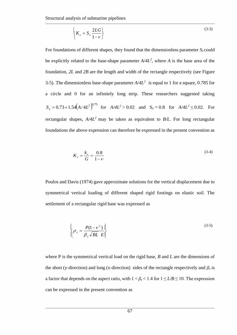
Structural analysis of submarine pipelines
67
−=
1
2LGSK zz
(3-3)
For foundations of different shapes, they found that the dimensionless parameter Sz could
be explicitly related to the base-shape parameter A/4L2, where A is the base area of the
foundation, 2L and 2B are the length and width of the rectangle respectively (see Figure
3-5). The dimensionless base-shape parameter A/4L2 is equal to 1 for a square, 0.785 for
a circle and 0 for an infinitely long strip. These researchers suggested taking
( ) 75.024/54.173.0 LAS z += for A/4L2 > 0.02 and Sz = 0.8 for A/4L2 ≤ 0.02. For
rectangular shapes, A/4L2 may be taken as equivalent to B/L. For long rectangular
foundations the above expression can therefore be expressed in the present convention as
−==
1
8.0
G
kK v
v
(3-4)
Poulos and Davis (1974) gave approximate solutions for the vertical displacement due to
symmetrical vertical loading of different shaped rigid footings on elastic soil. The
settlement of a rectangular rigid base was expressed as
−
=EBL
P
z
z
)1( 2
(3-5)
where P is the symmetrical vertical load on the rigid base, B and L are the dimensions of
the short (y-direction) and long (x-direction) sides of the rectangle respectively and βz is
a factor that depends on the aspect ratio, with 1 < βz < 1.4 for 1 ≤ L/B ≤ 10. The expression
can be expressed in the present convention as
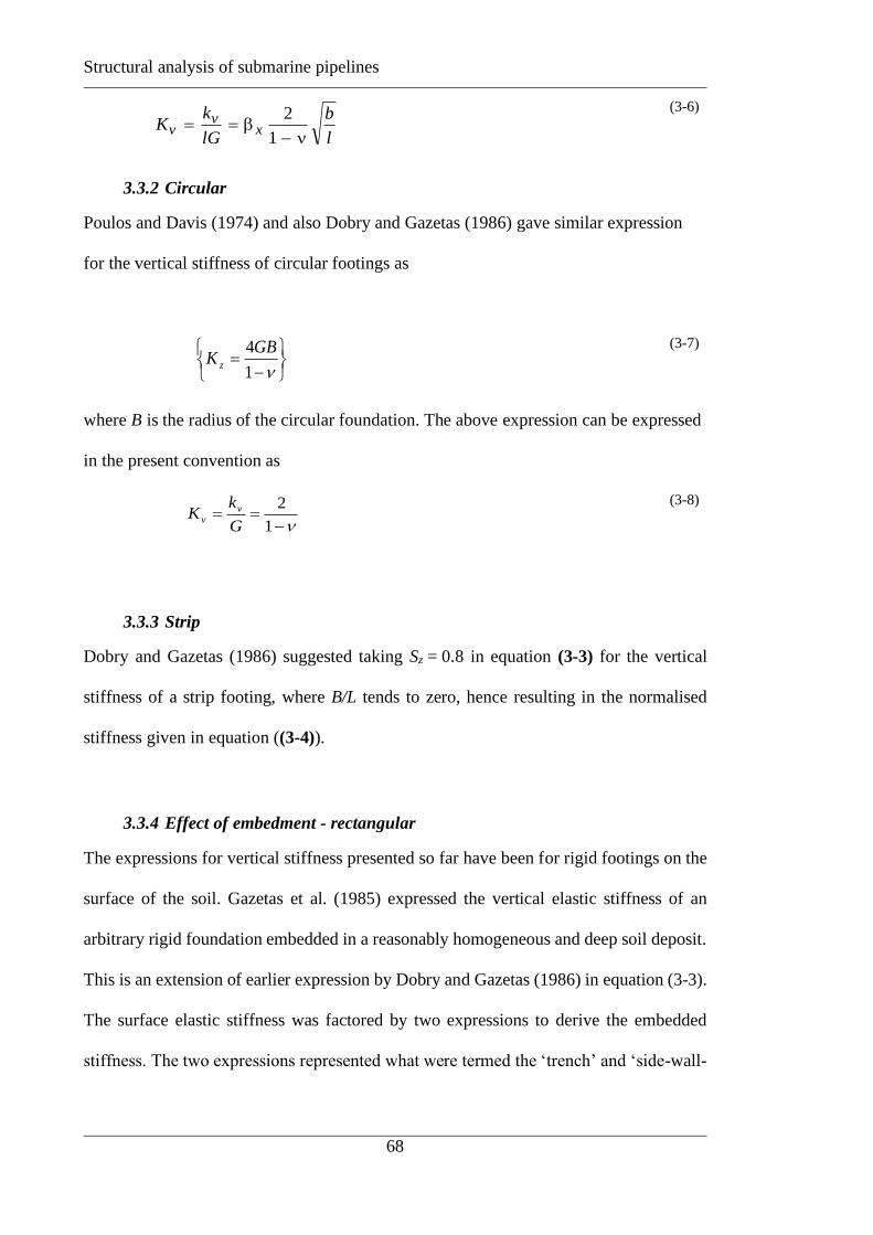
Structural analysis of submarine pipelines
68
l
b
lG
kK x
vv
−==
1
2
(3-6)
3.3.2 Circular
Poulos and Davis (1974) and also Dobry and Gazetas (1986) gave similar expression
for the vertical stiffness of circular footings as
−=
1
4GBK z
(3-7)
where B is the radius of the circular foundation. The above expression can be expressed
in the present convention as
−==
1
2
G
kK v
v
(3-8)
3.3.3 Strip
Dobry and Gazetas (1986) suggested taking Sz = 0.8 in equation (3-3) for the vertical
stiffness of a strip footing, where B/L tends to zero, hence resulting in the normalised
stiffness given in equation ((3-4)).
3.3.4 Effect of embedment - rectangular
The expressions for vertical stiffness presented so far have been for rigid footings on the
surface of the soil. Gazetas et al. (1985) expressed the vertical elastic stiffness of an
arbitrary rigid foundation embedded in a reasonably homogeneous and deep soil deposit.
This is an extension of earlier expression by Dobry and Gazetas (1986) in equation (3-3).
The surface elastic stiffness was factored by two expressions to derive the embedded
stiffness. The two expressions represented what were termed the ‘trench’ and ‘side-wall-

Structural analysis of submarine pipelines
69
contact’ effects, and were investigated separately. The final embedded vertical stiffness
was expressed as:
+
++
−=
3/2
219.01
43
41
21
11
1
2
b
sbz
embA
A
L
A
B
DLGSK
(3-9)
where Ab = is the area of the basement-soil contact surface, 2L and 2B are the length and
width of the rectangle circumscribed to the actual shape of the footing as shown in Figure
3-5. D is the embedment depth, d/2 is half the depth of side-wall contact (see Figure 3-6).
This may be approximately applied to the case of a pipeline of invert embedment w and
contact width B, with maximum w/B 0.5 for a pipeline half-embedded in the soil. In this
case, stiffness increases by a factor of 1.13 compared with a surface foundation.
+
++
−==
3/2
219.01
3
41
2
21
11
1 B
w
L
B
B
wS
G
kK zv
v
(3-10)
Similarly Pais and Kausel (1988) also expressed the static vertical elastic stiffness for an
embedded rectangular foundation as
( )
++=
8.0/
/
25.025.00.1 BE
BLKK o
V
s
V
(3-11)
where E/B is the embedment ratio. This expression can be converted into the present non-
dimensional form as:
( )
++=
8.0
_ /2/
25.025.00.1 bw
blKK Vembv
(3-12)
3.3.5 Pipe as half pile
As an alternative approach, a pipeline embedded by half its diameter, loaded vertically,
may be considered to have approximately half the lateral p-y stiffness at depths sufficient
to negate the surface effects for a pile in homogeneous soil. Analytical solutions for the
latter (e.g., Baguelin et al. 1977; Osman and Randolph 2012)for undrained conditions (ν

Structural analysis of submarine pipelines
70
= 0.5) suggest a p-y stiffness of four to five times the shear modulus of the soil G, leading
to an estimate for vertical pipeline stiffness of
25.2vK (3-13)
where the average of the suggested range is adopted.
3.3.6 Buried pipeline
Selvadurai (1985) presented buried-pipeline vertical elastic stiff-ness during ground
movement as
−==
1
3.1
G
kK v
v (3-14)
Matsubara and Hoshiya (2000) gave spring vertical stiffness for a buried pipeline as a
function of shear modulus G and ratio λ of an outer radius of assumed zero
displacement to the radius of the buried pipe, from which
e
v
vG
kK
log
2==
(3-15)
For λ = 10, Kv is 2.72.
3.3.7 Pipe on seabed – design guidelines
For a partially embedded pipeline, which is the main geometry of interest here, the
recommended practice (DNV 2019) suggests a vertical elastic stiffness derived from a
rectangular footing with L/B = 10 as
−=
1
88.0 GK v
(3-16)
Converting the above expression into the present dimensionless format leads to
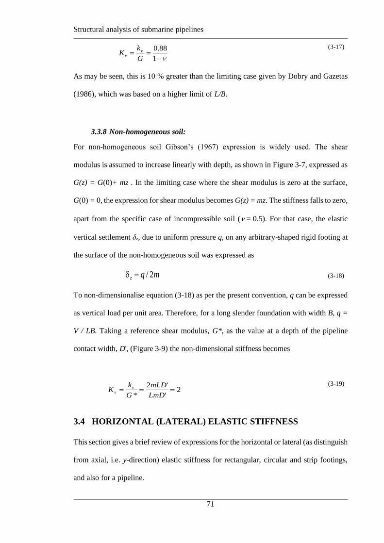
Structural analysis of submarine pipelines
71
−==
1
88.0
G
kK v
v
(3-17)
As may be seen, this is 10 % greater than the limiting case given by Dobry and Gazetas
(1986), which was based on a higher limit of L/B.
3.3.8 Non-homogeneous soil:
For non-homogeneous soil Gibson’s (1967) expression is widely used. The shear
modulus is assumed to increase linearly with depth, as shown in Figure 3-7, expressed as
G(z) = G(0)+ mz . In the limiting case where the shear modulus is zero at the surface,
G(0) = 0, the expression for shear modulus becomes G(z) = mz. The stiffness falls to zero,
apart from the specific case of incompressible soil ( = 0.5). For that case, the elastic
vertical settlement δz, due to uniform pressure q, on any arbitrary-shaped rigid footing at
the surface of the non-homogeneous soil was expressed as
mqz 2/= (3-18)
To non-dimensionalise equation (3-18) as per the present convention, q can be expressed
as vertical load per unit area. Therefore, for a long slender foundation with width B, q =
V / LB. Taking a reference shear modulus, G*, as the value at a depth of the pipeline
contact width, D', (Figure 3-9) the non-dimensional stiffness becomes
2'
'2
*===
LmD
mLD
G
kK v
v
(3-19)
3.4 HORIZONTAL (LATERAL) ELASTIC STIFFNESS
This section gives a brief review of expressions for the horizontal or lateral (as distinguish
from axial, i.e. y-direction) elastic stiffness for rectangular, circular and strip footings,
and also for a pipeline.
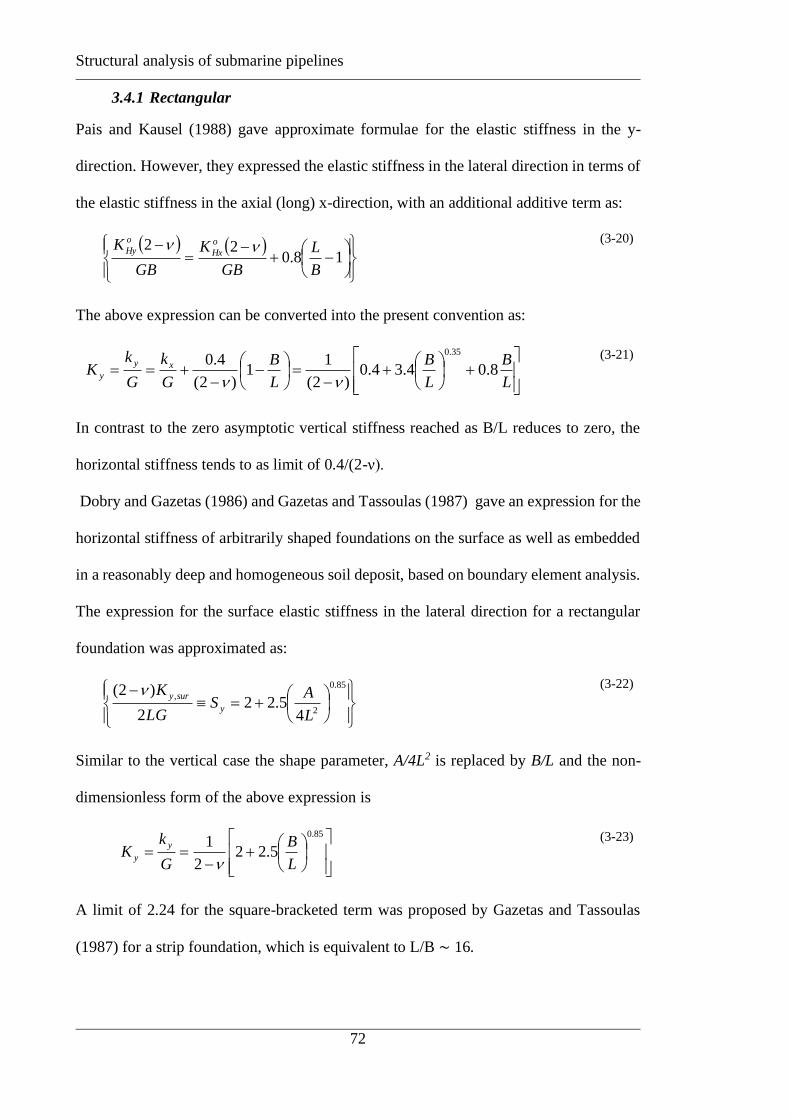
Structural analysis of submarine pipelines
72
3.4.1 Rectangular
Pais and Kausel (1988) gave approximate formulae for the elastic stiffness in the y-
direction. However, they expressed the elastic stiffness in the lateral direction in terms of
the elastic stiffness in the axial (long) x-direction, with an additional additive term as:
( ) ( )
−+
−=
−18.0
22
B
L
GB
K
GB
K o
Hx
o
Hy
(3-20)
The above expression can be converted into the present convention as:
+
+
−=
−
−+==
L
B
L
B
L
B
G
k
G
kK xy
y 8.04.34.0)2(
11
)2(
4.035.0
(3-21)
In contrast to the zero asymptotic vertical stiffness reached as B/L reduces to zero, the
horizontal stiffness tends to as limit of 0.4/(2-ν).
Dobry and Gazetas (1986) and Gazetas and Tassoulas (1987) gave an expression for the
horizontal stiffness of arbitrarily shaped foundations on the surface as well as embedded
in a reasonably deep and homogeneous soil deposit, based on boundary element analysis.
The expression for the surface elastic stiffness in the lateral direction for a rectangular
foundation was approximated as:
+=
− 85.0
2
,
45.22
2
)2(
L
AS
LG
Ky
sury
(3-22)
Similar to the vertical case the shape parameter, A/4L2 is replaced by B/L and the non-
dimensionless form of the above expression is
+
−==
85.0
5.222
1
L
B
G
kK
y
y
(3-23)
A limit of 2.24 for the square-bracketed term was proposed by Gazetas and Tassoulas
(1987) for a strip foundation, which is equivalent to L/B ∼ 16.

Structural analysis of submarine pipelines
73
Poulos and Davis (1974) gave an approximate solution for the horizontal displacement
due to symmetrical horizontal loading of different rigid footings on elastic foundation.
The displacement of a rectangular rigid footing was expressed as:
−
=EBL
Q
X
h
)1( 2
(3-24)
where Q is the uniform horizontal load on a rectangular surface with length L and width
B and βz is a factor depending on L/B and ν, with 0.69 < βx < 1.25 for 1 < L/B <10. This
leads to a stiffness of
L
B
G
kK z
y
y
−
==1
2 (3-25)
3.4.2 Circular
Poulos & Davis (1974) gave expression for the horizontal elastic stiffness of a rigid
circular footing bonded to the surface of a half space as:
( )
−
+−=
E
apxx
)1(16
)1(87
(3-26)
where px is the average applied pressure and expressed as horizontal load per unit area,
P/πa2, P being the load and a the radius of the circle. The above expression can be re-
written as per the present convention as
( )
87
116
−
−==
G
kK
y
y (3-27)
For the same condition Gazetas & Tassoulas (1987) expressed the elastic stiffness of a
circular footing as:
−=
2
8GRK y
(3-28)
where R is the radius of the footing. The above expression can be re-written in non-
dimensionless form as:

Structural analysis of submarine pipelines
74
−==
2
4
G
kK
y
y
(3-29)
3.4.3 Strip
For strip footings, Gazetas & Tassoulas (1987) gave the horizontal elastic stiffness as
−=
2
24.2
2
G
L
K y
(3-30)
The non-dimensional form of the above expression is given by
−==
2
24.2
G
kK
y
y (3-31)
3.4.4 Pipe on seabed – design guideline
DNV (2006) recommended an expression for the lateral elastic stiffness for pipelines as
( ) += 176.0 GK L (3-32)
The above expression can be re-written in non-dimensional form as
)1(76.0 +==G
kK
y
y (3-33)
3.4.5 Effect of embedment
The effect of embedment on the horizontal elastic stiffness of a rectangular footing was
investigated by Gazetas and Tassoulas (1987). The surface elastic stiffness, Ky,sur was
given by equation (3-19). Therefore, the overall expression was expressed as:
+
+==
40.0
2,, 52.0115.01L
A
B
h
B
DKIIKK w
surywalltresuryy
(3-34)
where D is the embedment, h is the side wall’s centre of gravity from top of the ground
as shown in Figure 3-8 and Aw is area of the sidewall soil interface. The above expression
can be re-written as:
+
+=
4.02
_ 252.012
15.01L
B
B
w
B
wKK yemby
(3-35)

Structural analysis of submarine pipelines
75
where w/B will be considered as 0.5 for a pipeline embedded to half a diameter. (in-
creasing stiffness by a factor of 1.15 assuming that B/L = 0).
Pais and Kausel (1988) expressed the static horizontal elastic stiffness for an embedded
rectangular footing as
( )
+++=
8.0/
/1
34.133.00.1 BE
BLKK o
H
s
H
(3-36)
where E/B is the embedment ratio and the same expression can be converted into present
non-dimensional form as
( )
+++=
8.0
_ /2/1
34.133.00.1 Bw
BLKK yemby
(3-37)
which leads to a maximum increase by a factor of 1.33 compared with a surface strip
footing, for an embedment of w/B = 0.5.
3.4.6 Pipe as half pile
As for vertical motion, a pipeline embedded by half its diameter, loaded laterally, is
similar in geometry to a half pile in homogeneous soil, loaded laterally. Again, due to
symmetry, the pipeline horizontal (lateral) stiffness is expected to be close to half the pile
lateral “p-y” stiffness. The horizontal pipeline stiffness would therefore be identical to
the vertical stiffness (equation (3-13).
3.5 AXIAL ELASTIC STIFFNESS
Published work on shallow foundations tends to focus on vertical and lateral response
(parallel to the short side), providing only limited information on axial response (parallel
to the long side). There are, however, a few expressions in the literature for the
longitudinal stiffness of rectangular footings. Some insight may also be gained from
solutions for axial loading of piles that consider a pipeline half-embedded in the soil to
be equivalent to half a pile.

Structural analysis of submarine pipelines
76
3.5.1 Rectangular
Gazetas and Tassoulas (1987) gave an expression for the longitudinal stiffness of a
surface rectangular foundation as a reduction in lateral stiffness: :
−
−−=
L
BGLKK surysurx 1
75.0
21.0,,
(3-38)
This can be re-written in non-dimensional form as
( )
−
−−==
L
BK
G
kK y
xx 1
75.02
21.0
3-39)
Pais and Kausel (1988) gave an expression for the dynamic axial elastic stiffness of a
rectangular footing as
( )
+
=
−4.28.6
265.00
B
L
GB
K Hx
(3-40)
The non-dimensional form of the above expression is given by
+
−==
L
B
L
B
G
kK x
x 2.14.3)2(
135.0
(3-41)
3.5.2 Embedment effect
The effect of embedment on the axial elastic stiffness of a rectangular footing was
considered by Gazetas & Tassoulas (1987), adjusting the stiffness for a surface footing
in a similar way as for the vertical and lateral stiffness. The resulting expression was
+
+==
40.0
2,, 52.0115.01L
A
B
h
B
DKIIKK w
surxwalltresurxx
(3-42)
The non-dimensionalised form of the above expression is given by

Structural analysis of submarine pipelines
77
+
+=
40.02
_ 252.012
15.01L
B
B
w
B
wKK xembx
(3-43)
where w/b will be considered as 0.5 for a pipeline embedded to half a diameter. .
Pais and Kausel (1988) derived the static elastic stiffness of an embedded rectangular
footing, with the expression for the stiffness given by
( )
+++=
8.0/
/1
34.133.00.1 BE
BLKK o
H
s
H (3-44)
The above equation can be expressed in current notation as
( )
+++=
8.0
_ /2/1
34.133.00.1 Bw
BLKK xembx
(3-45)
3.5.3 Pipeline as half pile
Considering a pipeline, embedded by half its diameter, as similar in nature to half of a
pile, the axial stiffness (per unit length) may be taken as identical to that customarily
assumed in load transfer analysis of piles. Randolph and Wroth (1978) expressed the
relationship between mobilised shear stress, 0 , and displacement, a, as
=D
G a
20
(3-46)
where D is the pile diameter. The parameter, , was expressed in terms of the pile length
(normalised by diameter) and Poisson’s ratio, but was typically about 4. The
corresponding relationship should also hold for a pipeline half embedded in
homogeneous soil. This would suggest an axial stiffness of
42
0
=
ax
G
DK
(3-47)
In order to compare this expression with others for rectangular foundations, the
coefficient 4 on the denominator should be replaced by , with (Horikoshi and Randolph,
1999)
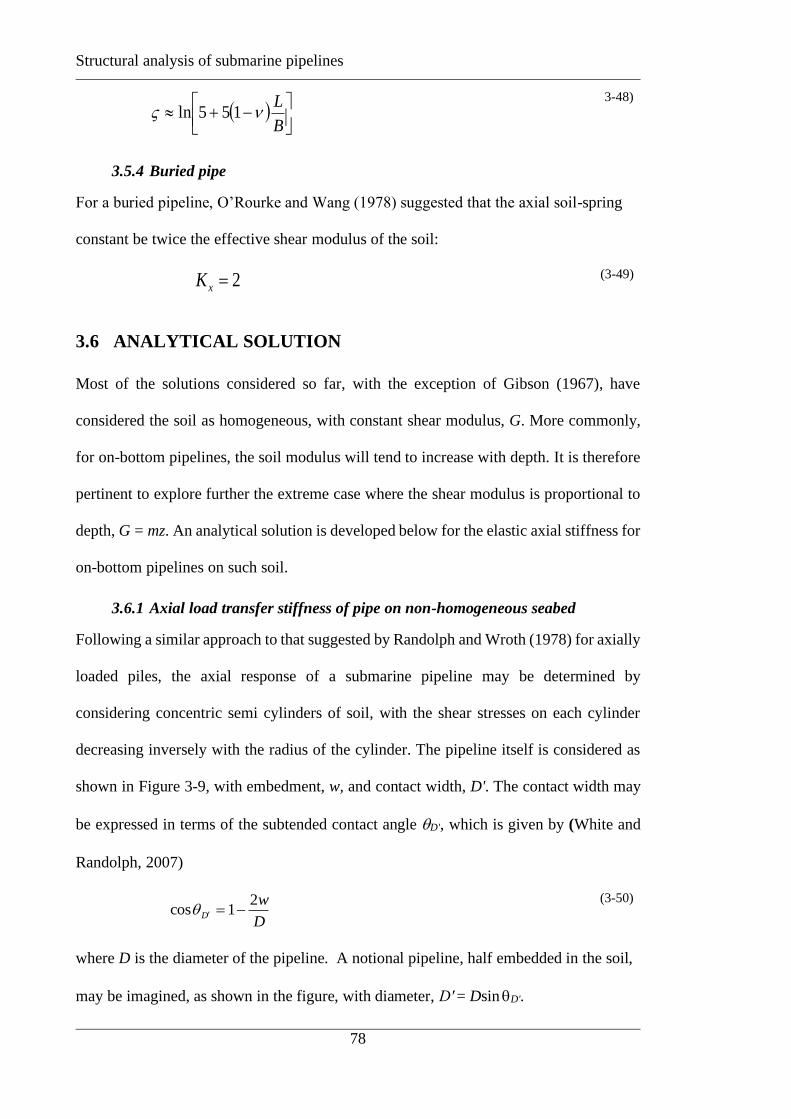
Structural analysis of submarine pipelines
78
( )
−+
B
L 155ln
3-48)
3.5.4 Buried pipe
For a buried pipeline, O’Rourke and Wang (1978) suggested that the axial soil-spring
constant be twice the effective shear modulus of the soil:
2=xK (3-49)
3.6 ANALYTICAL SOLUTION
Most of the solutions considered so far, with the exception of Gibson (1967), have
considered the soil as homogeneous, with constant shear modulus, G. More commonly,
for on-bottom pipelines, the soil modulus will tend to increase with depth. It is therefore
pertinent to explore further the extreme case where the shear modulus is proportional to
depth, G = mz. An analytical solution is developed below for the elastic axial stiffness for
on-bottom pipelines on such soil.
3.6.1 Axial load transfer stiffness of pipe on non-homogeneous seabed
Following a similar approach to that suggested by Randolph and Wroth (1978) for axially
loaded piles, the axial response of a submarine pipeline may be determined by
considering concentric semi cylinders of soil, with the shear stresses on each cylinder
decreasing inversely with the radius of the cylinder. The pipeline itself is considered as
shown in Figure 3-9, with embedment, w, and contact width, D'. The contact width may
be expressed in terms of the subtended contact angle D', which is given by (White and
Randolph, 2007)
D
wD
21cos −=
(3-50)
where D is the diameter of the pipeline. A notional pipeline, half embedded in the soil,
may be imagined, as shown in the figure, with diameter, D′ = Dsin D'.
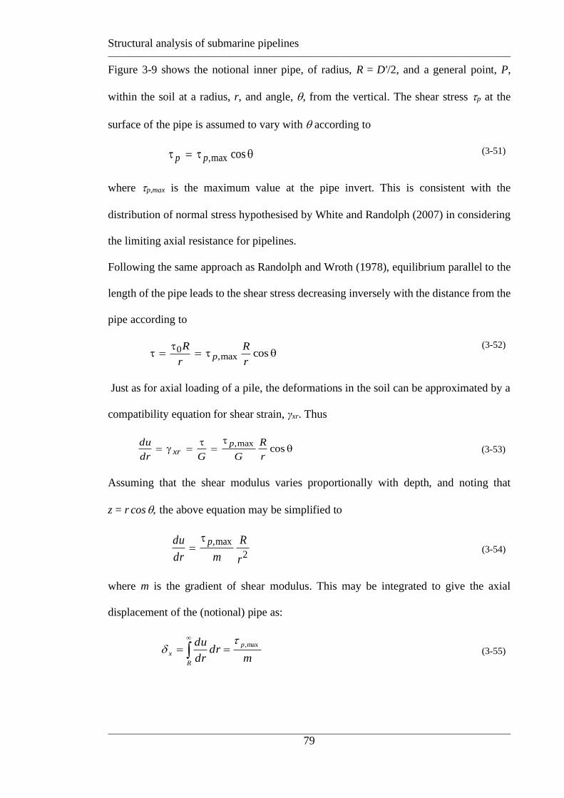
Structural analysis of submarine pipelines
79
Figure 3-9 shows the notional inner pipe, of radius, R = D'/2, and a general point, P,
within the soil at a radius, r, and angle, , from the vertical. The shear stress p at the
surface of the pipe is assumed to vary with according to
= cosmax,pp (3-51)
where p,max is the maximum value at the pipe invert. This is consistent with the
distribution of normal stress hypothesised by White and Randolph (2007) in considering
the limiting axial resistance for pipelines.
Following the same approach as Randolph and Wroth (1978), equilibrium parallel to the
length of the pipe leads to the shear stress decreasing inversely with the distance from the
pipe according to
=
= cosmax,0
r
R
r
Rp
(3-52)
Just as for axial loading of a pile, the deformations in the soil can be approximated by a
compatibility equation for shear strain, γxr. Thus
=
== cosmax,
r
R
GGdr
du pxr (3-53)
Assuming that the shear modulus varies proportionally with depth, and noting that
z = r cos the above equation may be simplified to
2
max,
r
R
mdr
du p= (3-54)
where m is the gradient of shear modulus. This may be integrated to give the axial
displacement of the (notional) pipe as:
mdr
dr
du p
R
x
max, ==
(3-55)

Structural analysis of submarine pipelines
80
Now integrating the value of τp around the pipe (ACB in Figure 3-10), leads to the
required axial stiffness (ratio of force per unit length to displacement) of
==
2/
0
max,
2/
0
cos22
dR
RdF
p
x
p
xx
(3-56)
Substituting for x from equation ((3-52)) gives
D
x
p
x
mDmRRF
sin22
max,=== (3-57)
The resulting axial stiffness may be normalised by the shear modulus at a level of half
the pipeline diameter, D, to give
−====
D
w
D
DF
mDK D
x
x 21arccossin2'
2sin22
(3-58)
Interestingly, this is exactly half the vertical stiffness derived for a pipeline embedded in
soil with modulus proportional to depth (Randolph, 2013). Alternatively, if the stiffness
is normalised by the shear modulus at a depth equal to the contact width, D', the non-
dimensional stiffness becomes
1sin
1=
=
xD
x
F
mDK (3-59)
This compares with the non-dimensional stiffness of Kx = /4 estimated from the half-
pile solution for the case of homogeneous soil (equation (3-44)). No pipe-soil slippage
was considered in developing the analytical model.
3.7 DISCUSSION
The aim of this chapter is to quantify the elastic stiffnesses of on-bottom pipelines and
the relationship between the stiffness in each direction (vertical, lateral and axial). It is
useful to compare the results of the literature review on elastic stiffnesses in each
direction, together with the approximate analytical solutions for axial stiffness of

Structural analysis of submarine pipelines
81
pipelines in non-homogeneous soil. The various values are plotted here for comparison.
In addition, relevant results from the finite element analyses presented later are also
shown. In many cases, the non-dimensional stiffnesses are a function of the aspect ratio,
which is plotted on a logarithmic scale.
Figure 3-11 shows the variation in nondimensional vertical elastic stiffness with aspect
ratio. For circular and square foundations, the Poulos and Davis (1974) and Dobry and
Gazetas (1986) solutions give similar values of 3.33. For a rectangular foundation, the
stiffnesses defined by Poulos and Davis (1974) and Pais and Kausel (1988) show similar
patterns although with diverging trends at high L/B (beyond the range of the original
studies), reducing to 0.46 and 0.83, respectively for L/B = 100 compared with the lower
limit of 1.33 proposed by Dobry and Gazetas (1986) for L/B ≥ 50. For an embedment
ratio of w/B = 0.5, the Gazetas et al. (1985) and Pais and Kausel (1988) solutions give
stiffness values of 1.5 and 1.03, respectively, for L/B = 100. For buried pipelines,
Matsubara and Hoshiya (2000) give a value of 2.7 for λ = 10 whereas Selvadurai (1985)
gives a value of 2.16 for L/B = 100. For a pipe on the seabed, the DNV (2019) guidelines
give a value of 1.46 nominally for L/B = 10, which matches closely with the Poulos and
Davis (1974) value. For nonhomogeneous soil with zero modulus at the soil surface but
a Poisson’s ratio of 0.5 rather than 0.4, the Gibson (1967) solution is equal to 2 for any
arbitrarily shaped rigid footing. The half-pile solution (Baguelin et al. 1977) gives a
slightly higher value of 2.25 for a pipe embedded by half a diameter in homogeneous soil.
The numerical solution from the finite-element analyses presented later is also plotted
here to facilitate comparison. For a half-embedded pipe (w/D = 0.5), nondimensional
vertical stiffness is found to vary from 3.0 (homogeneous soil) down to 2.62
(nonhomogeneous soil with G = mz), although both values are for a finite-layer depth of
6.25D and ν = 0.4.
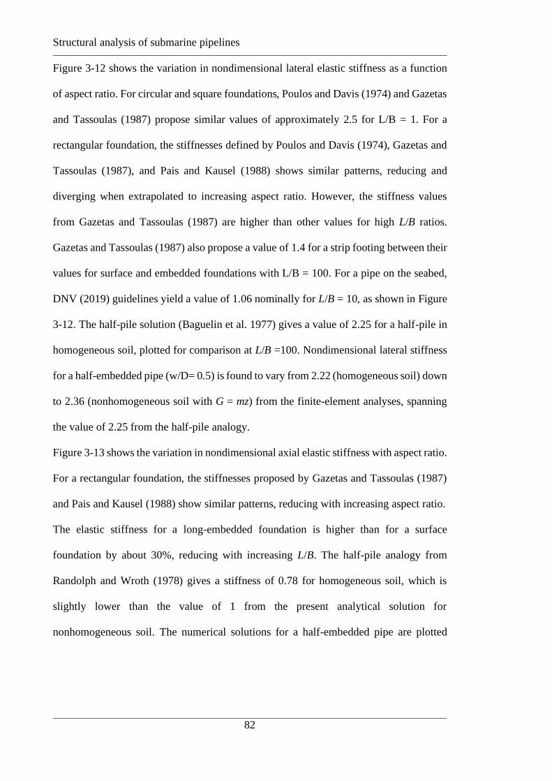
Structural analysis of submarine pipelines
82
Figure 3-12 shows the variation in nondimensional lateral elastic stiffness as a function
of aspect ratio. For circular and square foundations, Poulos and Davis (1974) and Gazetas
and Tassoulas (1987) propose similar values of approximately 2.5 for L/B = 1. For a
rectangular foundation, the stiffnesses defined by Poulos and Davis (1974), Gazetas and
Tassoulas (1987), and Pais and Kausel (1988) shows similar patterns, reducing and
diverging when extrapolated to increasing aspect ratio. However, the stiffness values
from Gazetas and Tassoulas (1987) are higher than other values for high L/B ratios.
Gazetas and Tassoulas (1987) also propose a value of 1.4 for a strip footing between their
values for surface and embedded foundations with L/B = 100. For a pipe on the seabed,
DNV (2019) guidelines yield a value of 1.06 nominally for L/B = 10, as shown in Figure
3-12. The half-pile solution (Baguelin et al. 1977) gives a value of 2.25 for a half-pile in
homogeneous soil, plotted for comparison at L/B =100. Nondimensional lateral stiffness
for a half-embedded pipe (w/D= 0.5) is found to vary from 2.22 (homogeneous soil) down
to 2.36 (nonhomogeneous soil with G = mz) from the finite-element analyses, spanning
the value of 2.25 from the half-pile analogy.
Figure 3-13 shows the variation in nondimensional axial elastic stiffness with aspect ratio.
For a rectangular foundation, the stiffnesses proposed by Gazetas and Tassoulas (1987)
and Pais and Kausel (1988) show similar patterns, reducing with increasing aspect ratio.
The elastic stiffness for a long-embedded foundation is higher than for a surface
foundation by about 30%, reducing with increasing L/B. The half-pile analogy from
Randolph and Wroth (1978) gives a stiffness of 0.78 for homogeneous soil, which is
slightly lower than the value of 1 from the present analytical solution for
nonhomogeneous soil. The numerical solutions for a half-embedded pipe are plotted

Structural analysis of submarine pipelines
83
forL/B = 100 in the figure and range from 1.06 for homogeneous soil down to 1.0 for G
= mz.
3.8 NUMERICAL SOLUTION
A series of small strain finite element (SSFE) analyses were performed in order to
validate the analytical solution for the elastic pipe-soil axial stiffness, and also derive
ratios between the vertical, lateral and axial stiffnesses. The analyses assumed the pipe
was “wished in place” at various embedment ratios (i.e. neglecting the pipe installation
process). The analytical and numerical results are compared and a parametric study
undertaken to explore the effects of soil parameters and embedment ratio on the elastic
stiffness. Simple expressions for the axial elastic stiffness for homogeneous and non-
homogenous soil are developed.
3.8.1 Geometry and mesh
A pipe diameter of D = 0.4 m was adopted, with both vertical and horizontal boundaries
placed at 2.5 m (10D) away from the centreline of the embedded portion of the pipe. This
was found to be sufficient to minimise boundary effects. The base of the soil model was
fixed in all three coordinate directions and the sides of the model were fixed in the
horizontal direction (Randolph et al., 2012). The portion of the pipe surface embedded in
the soil was treated as fully rough and bonded to the soil surface using the ‘tie constraint’,
which is computationally efficient and less prone to convergence problem than other
forms of contact (Zhang et al., 2011).
The rigid pipe section was also meshed (even though forced to displace as a rigid body)
with the number of elements around the periphery being equal to the corresponding
number of elements in the soil around the pipe (as necessary using tie constraints). A very
high Young’s modulus of 1011 MPa was adopted for the pipe to ensure essentially rigid
response. First order full integration hexahedral (C3D8) elements (as shown in Figure

Structural analysis of submarine pipelines
84
3-14) were used for both pipe and soil domains. Corresponding nodes on the two vertical
walls were tied together using the multi-point constraints available in ABAQUS, forcing
each node to have exactly the same degree of freedom. In this way, an infinitely long (but
rigid) pipe was modelled in order to evaluate the pipe-soil stiffness for any typical section
along the pipe.
3.8.2 Numerical analysis
The finite element analysis was performed using the commercial FE software ABAQUS
(Dassault Systèmes, 2007). Previous SSFE analysis of pipe-soil interaction on non-
homogeneous soil (e.g. Merifield et al., 2008; 2009) has mainly been restricted to vertical
and horizontal movement of the pipe, and axial soil-pipe interaction (especially in respect
of axial stiffness) has not been addressed properly in the literature.
For these analyses, the embedded portion of the pipe was modelled as a rigid body, with
load and displacement related to a single load reference point (LRP) at the centre of the
pipe section. As the stresses in the pipe are not relevant for this particular study,
consideration of a rigid pipe is computationally efficient. Pipes with different geometries
and embedment ratios (w/D) of 0.1, 0.2, 0.3, 0.4 and 0.5 were modelled for the analyses..
The shear modulus of the soil was assumed to increase linearly with depth, expressed as
G(z) = G(0)+ mz. In the limiting case where the shear modulus was zero at the surface,
G(0) = 0, the expression for shear modulus becomes G(z) = mz. Poisson’s ratio was taken
as = 0.4.
3.8.3 Verification of the model with V-H yield envelops
First, in order to validate the FE analyses, a fully bonded pipe-soil interface was
considered and V-H swipes were performed to establish the yield envelope in vertical-
horizontal space. Homogeneous soil with uniform shear strength of (su = 5 kPa) was
considered. Reaction forces were normalised by the shear strength of the soil and the
diameter of the pipe. Resulting envelopes were compared with those of Merifield et al.

Structural analysis of submarine pipelines
85
(2008). Exact matches were observed for all the embedment cases. The following Figure
3-15 shows the yield envelopes in V-H space for different initial embedment for the fully
bonded case.
Thereafter, numerical analyses were carried out to investigate the elastic response of
partially embedded pipes in all three directions.
3.8.4 Parametric study
A dimensionless parameter, , is introduced as:
')0(
'
mDG
mD
+=
(3-60)
For homogeneous soil, with m = 0, = and for the limiting case of stiffness
proportional to depth, with G(0) = 0, = The value of was varied from 0 to 1 with
an increment of 0.2, by keeping m constant (at 333 kPa/m) and varying G(0) for different
values of embedment for a pipe with G/su = 167. The elastic stiffnesses were then
normalised, by the value of G at a depth D′ (=G(D′) to eliminate the effect of the arbitrary
choice for G(0) and m.
It was found that the results of the parametric study could be fitted for both homogeneous
and non-homogeneous soils, expressing the non-dimensionless stiffness as (e.g. for the
axial direction)
b
xx
D
wa
DG
kK
=
=
2
)(
(3-61)
where, a and b are fitted constants, as functions of .
The values of a and b were found using a least squares method from the numerical results
and expressed as

Structural analysis of submarine pipelines
86
)1(3.015.0
)1(5.01
−+=
−+=
b
a
(3-62)
Figure 3-16 shows the normalised values of axial stiffnesses for different values of
along with the proposed fit. The analytical solution for = 1 is also plotted on the same
graph. The comparison between analytical and proposed fit improves with increasing
embedment. This is perhaps due to the diminishing difference between the true pipe
geometry and the equivalent pipe (Figure 3-9).Also, the proposed fit shows good
agreement with the numerical results.
Figure 3-17 shows the comparison between the actual and predicted axial stiffnesses for
= to covering homogeneous and non-homogenous soil conditions. Predicted
values are in good agreement with the actual stiffness.
In the following section finite element values of vertical and lateral stiffness, using the
same model and relationships as for the axial direction, are presented and compared with
the axial stiffness.
3.9 RELATION AMONGST AXIAL, VERTICAL AND LATERAL
ELASTIC STIFFNESSES OF ON-BOTTOM PIPELINE
The analytical expressions of lateral and vertical elastic stiffnesses were derived by
various researchers as discussed earlier in the chapter. However, the relationship between
axial and vertical or axial and lateral elastic stiffnesses was not addressed in the literature.
Therefore, this section aims to derive simple ratios of vertical versus axial elastic
stiffnesses and lateral versus axial elastic stiffnesses for the same group of input
parameters () used in the previous section.

Structural analysis of submarine pipelines
87
3.9.1 Comparison of elastic stiffnesses
Figure 3-18 shows the non-dimensional elastic stiffnesses in all the three directions for
homogeneous soil ( = 0), while Figure 3-19 shows corresponding results for the extreme
case of non-homogeneous soil with G(0) = 0 ( = 1).
Figure 3-20 illustrates the relationship between the vertical and axial and elastic
stiffnesses. The ratio is approximately constant at:
34.0=v
x
K
K
(3-63)
Similarly, Figure 3-21 shows the relationship between the lateral versus the axial elastic
stiffness where:
46.0=y
x
K
K
(3-64)
Just as for the axial case, the vertical and lateral elastic stiffnesses obtained numerically
may be estimated using equation (3-61) but with adjusted values of the parameter a to
reflect the above ratios. For completeness the values of a and b are summarised in Table
3-5 for all three directions.
Figure 3-22 and Figure 3-23 show the comparison between the actual and predicted
vertical and lateral stiffnesses respectively for = to covering the full range of
homogeneous and non-homogenous soil conditions. Predicted values are in good
agreement with the actual stiffness for both vertical and lateral loading, although with
slightly greater scatter for the former.
The higher value of vertical stiffness for homogeneous soil modulus may be attributed,
at least partly, to the limited layer depth modelled numerically. However, other studies of
strip foundation vertical stiffness suggest that this limited mesh extent is likely to raise
the stiffness by only ~ 15% (Sloan & Randolph 1982, Bell et al. 1992, Yan et al. 2011).
Therefore, the discrepancy evident in Figure 3-11 at L/B = 100 between the FE results
and the other relationships is because of their inaccuracy when extrapolated to higher L/B.

Structural analysis of submarine pipelines
88
For the lateral and axial cases, the deformation is restricted to a shallower region, and any
influence of the mesh extent is ignored.
The corresponding ratio, Ky/Kv, therefore averages 0.75. The largest outliers from each
set of ratios are those for the extreme non-homogeneous condition with G0 = 0, hence
= 1, for which the averages for the data at different embedment are about 10 % higher
than the overall averages indicated in Figure 3-24. Given the challenges of estimating
suitable ‘elastic’ shear modulus values for soil, the spread of stiffness ratios is acceptably
narrow.
3.10 CONCLUSIONS
Values of elastic stiffness for on-bottom pipelines have not been well defined in the
literature. However, based on previous studies for shallow foundations and present
analytical and numerical analyses approximate relationships for the stiffnesses and their
relative magnitudes have been proposed. An analytical model was presented to predict
the axial stiffness, validated through numerical analysis. The proposed form of
normalisation of the stiffness gave an almost constant value of unity, independent of
embedment or degree of soil non-homogeneity. Numerical analysis was used to conduct
a parametric study to evaluate corresponding stiffnesses in the horizontal and vertical
directions. These were found to be rather higher than values obtained by extrapolating
solutions for surface or shallowly embedded rectangular foundations.
Stiffness ratios of axial to lateral (Kx/ Ky) and axial to vertical (Kx/Kv) were evaluated and
found to show relatively minor variations with either embedment or non-homogeneity.
Average ratios of 0.34 and 0.46 were obtained (giving an average of 0.75 for Ky/Kv).
Generalised expressions were derived to evaluate the axial, lateral and vertical stiffnesses
directly as functions of w/D and . Overall, a robust systematic approach for selecting the
elastic stiffnesses of pipeline-soil interaction is to first evaluate the normalised axial
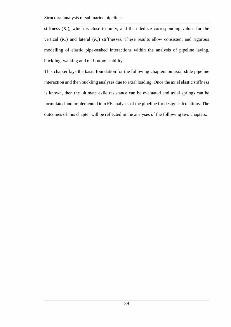
Structural analysis of submarine pipelines
89
stiffness (Kx), which is close to unity, and then deduce corresponding values for the
vertical (Kv) and lateral (Ky) stiffnesses. These results allow consistent and rigorous
modelling of elastic pipe-seabed interactions within the analysis of pipeline laying,
buckling, walking and on-bottom stability.
This chapter lays the basic foundation for the following chapters on axial slide pipeline
interaction and then buckling analyses due to axial loading. Once the axial elastic stiffness
is known, then the ultimate axile resistance can be evaluated and axial springs can be
formulated and implemented into FE analyses of the pipeline for design calculations. The
outcomes of this chapter will be reflected in the analyses of the following two chapters.
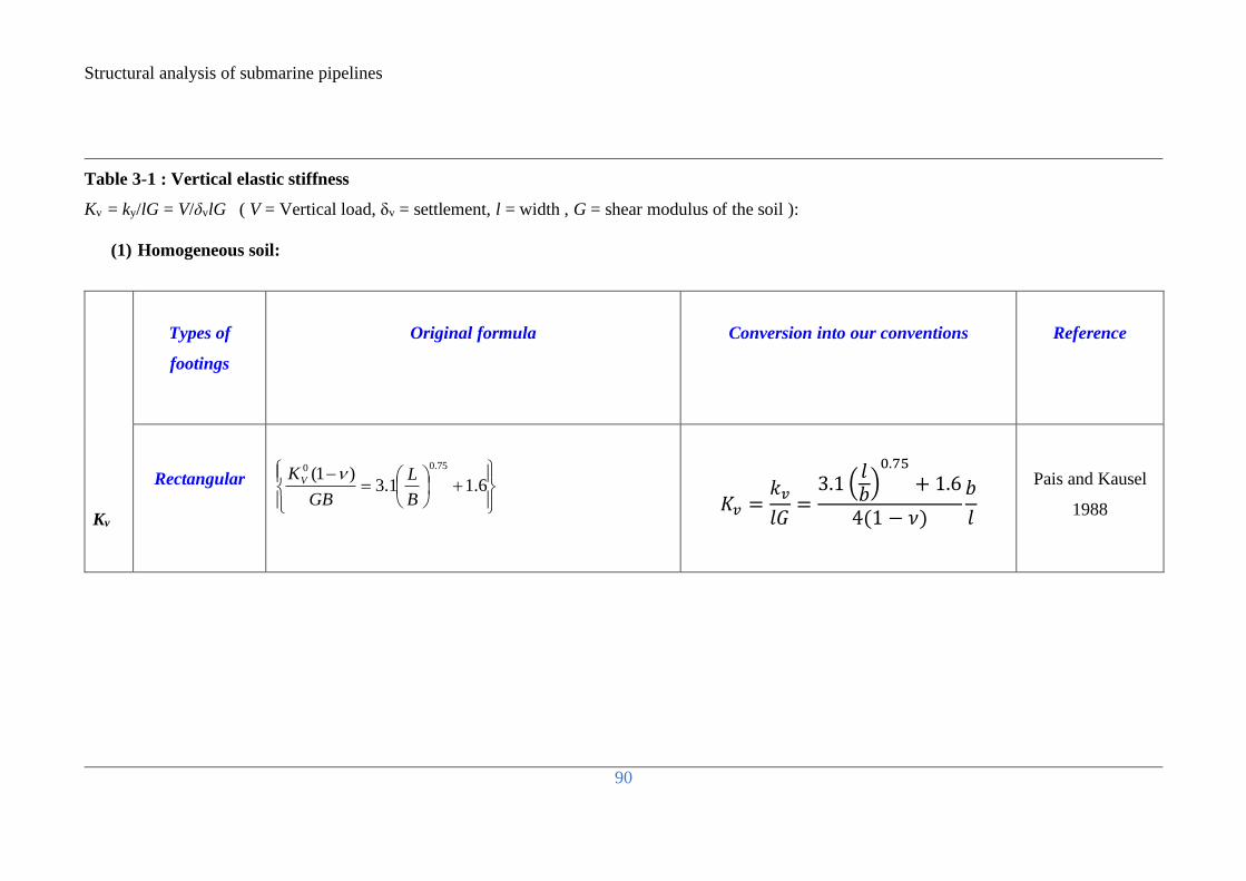
Structural analysis of submarine pipelines
90
Table 3-1 : Vertical elastic stiffness
Kv = ky/lG = V/δvlG ( V = Vertical load, δv = settlement, l = width , G = shear modulus of the soil ):
(1) Homogeneous soil:
Kv
Types of
footings
Original formula
Conversion into our conventions
Reference
Rectangular
+
=
−6.11.3
)1(75.00
B
L
GB
KV
𝐾𝑣 =𝑘𝑣
𝑙𝐺=
3.1 (𝑙𝑏
)0.75
+ 1.6
4(1 − 𝜈)
𝑏
𝑙
Pais and Kausel
1988
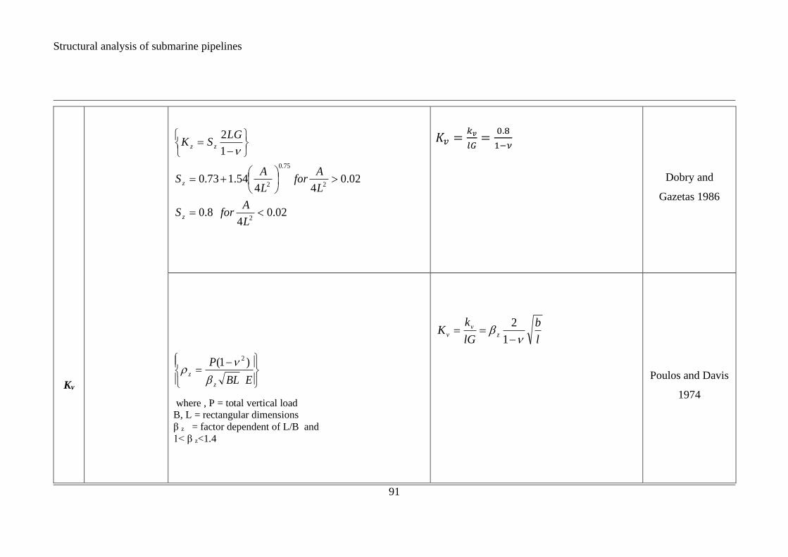
Structural analysis of submarine pipelines
91
Kv
02.04
8.0
02.044
54.173.0
1
2
2
2
75.0
2
=
+=
−=
L
AforS
L
Afor
L
AS
LGSK
z
z
zz
𝐾𝑣 =𝑘𝑣
𝑙𝐺=
0.8
1−𝜈
Dobry and
Gazetas 1986
−
=EBL
P
z
z
)1( 2
where , P = total vertical load B, L = rectangular dimensions
β z = factor dependent of L/B and
1< β z<1.4
l
b
lG
kK z
vv
−==
1
2
Poulos and Davis
1974

Structural analysis of submarine pipelines
92
Kv
Circular
−=
1
4GBK z
where B is equal to the radius of the circle
−==
1
2
lG
kK v
v
Dobry and
Gazetas 1986
&
−=E
apavz )1(
2
2
−===
1
2
Gb
k
Ga
PK v
w
v Poulos and Davis
1974
Strip
−=
1
8.0
2
G
L
K z
−==
1
8.0
lG
kK v
v
Dobry and
Gazetas 1986

Structural analysis of submarine pipelines
93
Pipe on seabed
−=
1
88.0 GK v
where KV =V/Δv and V is the incremental vertical force
between pipe and soil per unit length of pipe, and Δv is the
associated incremental vertical displacement of the pipe.
−==
1
88.0
lG
kK v
v
DNV(2019)
Rectangular
with
embedment
+
++
−=
3/2
219.01
43
41
21
11
1
2
b
sbz
embA
A
L
A
B
DLGSK
where, D = embedment depth
As = area of the sidewall soil interface = D x 2L
Ab = area of the base = 2L x 2B
+
++
−=
==
3/2
_
_
219.01
3
41
2
21
11
1 b
w
l
b
b
wS
lG
kK
z
embv
embv
w is the embedment depth
Gazetas , Dobry
& Tassoulas
1985
( )
++=
8.0/
/
25.025.00.1 BE
BLKK o
V
s
V
where E/B is the embedment ratio
( )
++=
8.0
_ /2/
25.025.00.1 bw
blKK Vembv
w is the embedment depth
Pais and Kausel
1988

Structural analysis of submarine pipelines
94
(2) Non-homogeneous soil
Kv
Arbitrary shape
mqv 2/=
Where q = Load / area
G(z) = mz
D
D
lG
kK v
v
= 4
*
Gibson 1967

Structural analysis of submarine pipelines
95
Table 3-2 : Lateral elastic stiffness
Ky = ky/lG = H/δylG ( H = Horizontal load, δy = lateral displacement, l = length , G = shear modulus of the soil )
(3) Homogeneous soil:
Ky
Rectangular
( ) ( )
−+
−=
−18.0
22 00
B
L
GB
K
GB
Kxy
)2(
14.0
−
−
+==l
b
lG
k
lG
kK xy
y
Pais and Kausel
1988
+=
− 85.0
2
,
45.22
2
)2(
L
AS
LG
Ky
sury
−
+
==2
5.22
85..0
l
b
lG
kK
y
y
Gazetas and
Tassoulas 1987
−
=EBL
Q
X
h
)1( 2
where Q = total horizontal load
B, L = rectangular dimensions
β z = factor dependent of L/B and ν 0.692< β x<1.25
𝐾𝑦 =𝑘𝑦
𝑙𝐺= 𝛽
2
1 − 𝜈√
𝑏
𝑙
Poulos and
Davis 1974

Structural analysis of submarine pipelines
96
Ky
Circular
−=
2
8GRK y
−==
2
4
lG
kK
y
y
Gazetas and
Tassoulas 1987
( )
−
+−=
E
apxx
)1(16
)1(87
where
px = average applied pressure, P/πa2
a = radius of the circle
−==
2
4
lG
kK
y
y
Poulos and
Davis 1974
Strip
−=
2
24.2
2
G
L
K y
−==
2
24.2
lG
kK
y
y
Gazetas and
Tassoulas 1987
Pipe on seabed
( ) += 176.0 GK L
Where KL=FL/ΔδL, where ΔFL is the incremental
horizontal force between pipe and soil per unit length
)1(76.0 +==lG
kK
y
y DNV(2002)

Structural analysis of submarine pipelines
97
Ky
of pipe, and ΔδL is the associated incremental
horizontal displacement of the pipe.
Rectangular
with embedment
+
+=
40.0
2, 52.0115.01L
A
B
h
B
DKK w
suryy
Where, D = embedment depth
h = side wall’s centre of gravity from top of the ground
Aw = area of the sidewall soil interface = D x 2L
+
+=
=
40.02
_
252.012
15.01l
w
b
d
b
wK
K
y
emby
Gazetas and
Tassoulas 1987
( )
+++=
8.0/
/1
34.133.00.1 BE
BLKK o
H
s
H
( )
+++=
8.0
_ /2/1
34.133.00.1 bw
blKK yemby
Pais and Kausel
1988

Structural analysis of submarine pipelines
98
Table 3-3 : Axial elastic stiffness
Kx = kx/lG = F/δx lG ( F = Axial load, δx= axial displacement, l= width , G = shear modulus of the soil ):
(4) Homogeneous soil
Kx
Rectangular
( )
+
=
−4.28.6
265.00
B
L
GB
K Hx
+
−==
l
b
l
b
lG
kK x
x 2.14.3)2(
135.0
Pais and Kausel 1988
−
−−=
L
BGLKK surysurx 1
75.0
21.0,,
( )
−
−−==
l
b
lG
k
lG
kK
yxx 1
75.02
21.0
Gazetas and Tassoulas
1987
Rectangular
with embedment
+
+=
==
40.0
2,
,
52.0115.01L
A
B
h
B
DK
IIKK
w
surx
walltresurxx
Where D = embedment depth
h = side wall’s centre of gravity from top of the
ground
Aw = area of the sidewall soil interface = D x 2L
+
+=
=
40.02
_
252.012
15.01l
b
b
w
b
wK
K
x
embx
Gazetas and Tassoulas
1987
Structural analysis of submarine pipelines
99
( )
+++=
8.0/
/1
34.133.00.1 BE
BLKK o
H
s
H
( )
+++=
8.0
_ /2/1
34.133.00.1 bw
blKK yemby Pais and Kausel 1988
Pipeline as half
pile
=DG
X
20
Where D = Pile diameter
ζ = side wall’s centre of gravity from top of the
ground
Aw = area of the sidewall soil interface = D x 2L
42
0
=
x
xG
DK
To compare this with rectangular foundation
4 is replaced with,
( )
−+
b
l155ln (Horikoshi & Randolph
1999)
Randolph and Wroth
(1978)

Structural analysis of submarine pipelines
100
(5) Non homogeneous soil with embedment
Kx
Pipe on seabed
'sin' D
x
x mDmDF
k
===
Where F = axial resistance per unit length δx= axial displacement
Dʹ = embedded diameter
D = diameter of the pipe
θD’ = embedment angle
1sin
1
21sin22sin22
==
−=
===
xD
x
D
x
x
F
mDK
or
D
warcCos
D
DF
mDK
analytical
solution
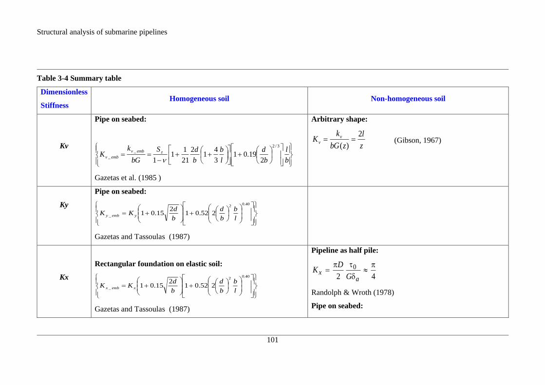
Structural analysis of submarine pipelines
101
Table 3-4 Summary table
Dimensionless
Stiffness Homogeneous soil Non-homogeneous soil
Kv
Pipe on seabed:
+
++
−==
b
l
b
d
l
b
b
dS
bG
kK zembv
embv
3/2
_
_2
19.013
41
2
21
11
1
Gazetas et al. (1985 )
Arbitrary shape:
z
l
zbG
kK v
v
2
)(== (Gibson, 1967)
Ky
Pipe on seabed:
+
+=
40.02
_ 252.012
15.01l
b
b
d
b
dKK yemby
Gazetas and Tassoulas (1987)
Kx
Rectangular foundation on elastic soil:
+
+=
40.02
_ 252.012
15.01l
b
b
d
b
dKK xembx
Gazetas and Tassoulas (1987)
Pipeline as half pile:
42
0
=
ax
G
DK
Randolph & Wroth (1978)
Pipe on seabed:

Structural analysis of submarine pipelines
102
−=
−===
D
warcCos
z
DK
D
warcCos
z
l
z
l
bzG
kK
x
Dx
x
21sin
21sinsin)(
'

Structural analysis of submarine pipelines
103
Table 3-5: Summary table for various stiffnesses
Axial Vertical Lateral b
xx
D
wa
DG
kK
=
2
)(
b
vv
D
wa
DG
kK
=
2
)(
b
y
yD
wa
DG
kK
=
2
)(
)1(3.015.0
)1(5.01
−+=
−+=
b
a
)1(3.015.0
)1(5.0185.2
−+=
−+=
b
a
)1(3.015.0
)1(5.0112.2
−+=
−+=
b
a
Structural analysis of submarine pipelines
104
Reference:
Baguelin, F, Frank, R, Said, Y.H. (1977). Theoretical study of lateral reaction
mechanism of piles. Geotechnique 27(3): 405-434.
Bell, R. W., Houlsby, G. T., and Burd, H. J. (1992). Finite element analysis of
axisymmetric footings subjected to combined loads. Computer Methods and
Advances in Geomechanics, 3, Balkema, 1992, 1765-1770.
Dassault Systèmes (2007) Abaqus analysis users’ manual, Simula Corp, Providence, RI,
USA.
DNV∙GL (2019). Recommended Practice RP-F114. Pipe-soil interaction for submarine
pipelines.
Dobry, R. & Gazetas, G. (1986).Dynamic response of arbitrary shaped foundations.
Journal of Geotechnical Engineering, ASCE, Vol. 112, No. 2, February, 109-
135.
Gazetas, G., Dobry, R. & Tassoulas, J. L. (1985). Vertical response of arbitrarily shaped
embedded foundations. Journal of Geotechnical Engineering, ASCE, Vol. 111,
No. 6, June, 750-771.
Gazetas, G. & Tassoulas, J. L. (1987).Horizontal stiffness of arbitrary shaped embedded
foundations. Journal of Geotechnical Engineering, ASCE, Vol. 113, No. 5, May,
440-457.
Gibson, R. E. (1967). Some results concerning displacement and stresses in a non-
homogeneous elastic half-space. Géotechnique, 17: 58-67.
Hodder, M. S. & Cassidy, M. J. (2010). A plasticity model for predicting the vertical
and lateral behaviour of pipelines in clay soils. Géotechnique 60, No. 4, 247-
263.

Structural analysis of submarine pipelines
105
Horikoshi, K., & Randolph, M. F (1999). Estimation of overall settlement of piles rafts.
Soils and Foundations. Japanese Geotechnical Society. Vol. 39, No. 2, April, 59-
68.
Matsubara, K., & Hoshiya, M. (2000). Soil spring constants of buried pipelines for
seismic design. Journal of Engineering Mechancis, ASCE, 126, No. 1, 76-83.
Merifield, R. S., White, D. J. & Randolph, M. F. (2008). The ultimate undrained
resistance of partially embedded pipelines. Géotechnique 58, No. 6, 461-470.
Merifield R. S., White, D. J. & Randolph, M. F. (2009). Effect of surface heave on
response of partially embedded pipelines on clay. J. Geotech. Geoenviron.
Engng, ASCE 135, No. 6, 819-829.
O’Rourke, M. J., &Wang, L. R. L. (1978). Earthquake response of buried pipelines.
Proceedings of the Special Conference on Earthquake Engineering and Soil
Dynamics, Pasadena, California, ASCE, 720-731.
Osman, A.S. and Randolph, M.F. (2012). An analytical solution for the consolidation
around a laterally loaded pile. Int. J. of Geomechanics, ASCE, 12(3), 199-208.
Pais, A. & Kausel, P. (1988).Approximate formulas for dynamic stiffness of rigid
foundations. Soil Dynamics and Earthquake Engineering, Vol. 7, No. 4, 213-
227.
Poulos, H.G. & Davis, E.H. (1974).Elastic solutions for soil and rock mechanics. John
Wiley & Sons, Inc.
Randolph, M. F. (2013). Analytical contribution to offshore geotechnical engineering.
McClelland Lecture. Proc. 18th International Conference on Soil Mechanics and
Geotechnical Engineering, Paris, 85-105
Randolph, M. F., White, D. J. and Yan, Y. (2012). Modelling the axial soil resistance on
deep-water pipelines. Géotechnique. 62, No. 9, 837-846

Structural analysis of submarine pipelines
106
Randolph, M. F. and Wroth, C. P. (1978). Analysis of deformation of vertically loaded
piles. J. Geotech. Engng Div. Am. Soc. Civ. Engrs 104, GT 12, 1465-1488
Salvadurai A. P. S. (1985). Soil-pipeline interaction during ground movement. Civil
Engineering in the Arctic Offshore, ASCE Conference, United States, 763-773.
Sloan, S.W. and Randolph, M. F. (1982). Numerical prediction of collapse loads using
finite element methods. Int. J. Numer. Anal. Meth. Geomech., 6, 17-76.
Tian, Y., Cassidy, M. J., & Gaudin, C. (2010). Advancing pipe-soil interaction models
through geotechnical centrifuge testing in calcareous sand. Applied Ocean
Research, DOI: 10.1016/j.apor.2010.06.002
Tian, Y. & Cassidy, M. J. (2010). A pipe-soil interaction model incorporating large
lateral displacement in calcareous sand. Journal of Geotechnical Engineering,
ASCE, DOI: 10.1061/(ASCE)GT.1943-5606.0000428
White, D. J. & Randolph, M. F. (2007). Seabed characterisation and models for
pipeline-soil interaction. International Journal of Offshore and Polar
Engineering, Vol. 17, No. 3, 193-204.
Yan Y. White D.J. & Randolph M.F. (2011). Penetration resistance and stiffness factors
in uniform clay for hemispherical and toroidal penetrometers. International
Journal of Geomechanics, 11:263-275
Zhang, Y., Bienen, B., Cassidy, M. J., & Gourvenec, S. M. (2011). The undrained
bearing capacity of a spudcan foundation under combined loading in soft clay.
Marine Structure, Vol. 24, 459-477.

Structural analysis of submarine pipelines
107
Figures:
Figure 3-1: Idealisation of the pipeline on nonlinear seabed by nonlinear springs
attached to the pipeline
Figure 3-2 Loads and displacement of a pipe element

Structural analysis of submarine pipelines
108
Figure 3-3: Dimension considered for the present study
Figure 3-4 Dimensions of embedded footing by Pais and Kausel, 1988
Figure 3-5 Dimensions of embedded footing by Dobry and Gazetas, 1986
Figure 3-6: Dimensions of embedded footing for vertical stiffness by Gazetas, Dobry,
and Tassoulas, 1985

Structural analysis of submarine pipelines
109
Figure 3-7: Variation of shear modulus in linear and nonlinear soil, Gibson 1967
Figure 3-8 Dimensions of embedded footing by Gazetas and Tassoulas , 1986

Structural analysis of submarine pipelines
110
Figure 3-9: Pipe embedment geometry
Figure 3-10: Deformation of soil below the pipe
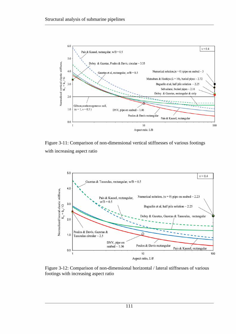
Structural analysis of submarine pipelines
111
Figure 3-11: Comparison of non-dimensional vertical stiffnesses of various footings
with increasing aspect ratio
Figure 3-12: Comparison of non-dimensional horizontal / lateral stiffnesses of various
footings with increasing aspect ratio

Structural analysis of submarine pipelines
112
Figure 3-13: Comparison of non-dimensional horizontal / axial stiffnesses of various
footings with increasing aspect ratio
Figure 3-14: Finite element model used to estimate the axial stiffness

Structural analysis of submarine pipelines
113
Figure 3-15: Failure envelopes in vertical-horizontal space
Figure 3-16: Normalised axial stiffnesses for different values of
0
0.5
1
1.5
2
2.5
3
3.5
4
0 1 2 3 4 5 6 7
No
rmal
ise
d la
tera
l re
sist
ance
, H/s
uD
Normalised vertical resistance, V/suD
w/D = 0.1 to 0.5
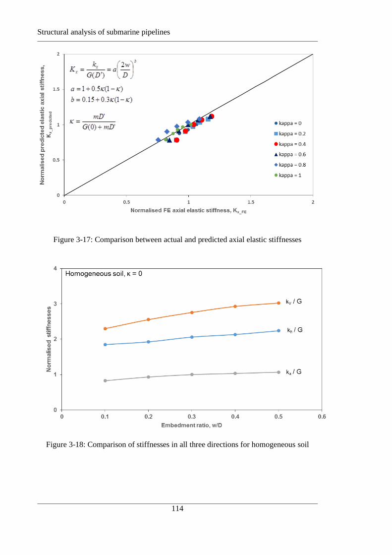
Structural analysis of submarine pipelines
114
Figure 3-17: Comparison between actual and predicted axial elastic stiffnesses
Figure 3-18: Comparison of stiffnesses in all three directions for homogeneous soil

Structural analysis of submarine pipelines
115
Figure 3-19: Comparison of stiffnesses in all three directions for non-homogeneous soil
Figure 3-20: Ratio between vertical Vs axial elastic stiffnesses

Structural analysis of submarine pipelines
116
Figure 3-21: Ratio between lateral Vs axial elastic stiffnesses
Figure 3-22: Comparison between actual and predicted vertical elastic stiffnesses

Structural analysis of submarine pipelines
117
Figure 3-23: Comparison between actual and predicted lateral elastic stiffnesses
Figure 3-24: Ratios of axial to lateral and vertical stiffnesses
0.20
0.25
0.30
0.35
0.40
0.45
0.50
0.55
0.60
0 0.1 0.2 0.3 0.4 0.5 0.6
Rat
ios
of
axia
l to
lat
eral
an
d v
erti
cal
stif
fnes
s
Embedment ratio, w/D
Kx / Kv = 0.34
Kx / Ky = 0.46
= 00.2
0.40.60.81
Structural analysis of submarine pipelines
118

Structural analysis of submarine pipelines
119
ANALYTICAL SOLUTION OF
SUBMARINE PIPELINE AND SLIDE INTERACTION
4.1 INTRODUCTION
The offshore oil and gas industry commonly operates in deepwater, beyond the
continental shelf, where infrastructure is vulnerable to a number of geohazards including
submarine landslides, mud and volcanoes, seismicity, shallow gas and gas hydrates
(Kvalstad et al. 2001). One of the most significant geohazards on the continental slope is
the threat of submarine landslides, which typically originate from the shelf-break but may
run out several kilometres into development zones or across pipeline routes. Submarine
pipelines are the safest and most economical mode of transporting hydrocarbon products
from deepwater to the shore. Hence, such pipelines are more exposed to impact risk from
submarine slides than other seabed infrastructure. Therefore, geohazard assessment, and
in particular quantifying the response of pipelines to impact from submarine debris flow,
has become a critical issue for the industry.
This chapter focuses on developing an analytical solution for axial submarine slide
pipeline interaction. The submarine slide was considered as a moving block of constant
shear strength along the longitudinal direction of the pipeline, hence developing
compressive forces in the downstream pipeline and tensile forces in the upstream of the
pipeline. The axial loading on the pipeline from the submarine slide movement can be
assessed using two different approaches: (1) geotechnical and (2) fluid dynamics. The
latter approach was not included in this thesis. Here, a geotechnical approach will be
considered to analyse the effect of submarine slides on the pipelines.

Structural analysis of submarine pipelines
120
The chapter describes the derivation of a solution for the axial load and deformation of
an elastic pipeline laid on a seabed, assuming a linear elastic – perfectly plastic t-z
response (outside the slide zone). The effect of the submarined axial slide is represented
by a uniform axial load (force per unit length) over a defined length of the pipeline. In the
analysis, buckling of the on-bottom pipeline due to the axial slide loading downstream of
the slide has been neglected. However, the peak axial load experienced by a given
pipeline due to different slide loading cases and t-z responses were compared with the
critical buckling load of the pipeline as calculated by classical buckling theory.
4.2 PROBLEM DEFINITION AND BACKGROUND LITERATURE
To investigate the axial slide impact on the pipeline the frictional force developed on the
pipeline due to the slide movement and seabed needs to be calculated. The following
sections start by reviewing previous work on load transfer from the slide (active loading)
and frictional resistance of the seabed (passive resistance). Thereafter, a proposed method
to estimate the net resistance on the pipe due to slide movement along the length (parallel
to the pipeline axis) is identified along with the boundary conditions. However, the case
where the pipe is inside the mudflow with a moving soil below the pipe invert has been
kept out of this scope.
4.2.1 Active slide loading – geotechnical approach
As stated above (in Section 4.1) only geotechnical approaches are considered in this
chapter for loading on a submarine pipeline due to slide movement parallel and normal
to the pipe. Buckling and other forms of failure of the pipe is considered later in the thesis.
The active force on any infrastructure on the seabed may be expressed in terms of the
shear strength of the sliding soil mass. A typical expression is given as (Zakeri, 2009)

Structural analysis of submarine pipelines
121
AksFslideun _
=
(4-1)
where su_slide is the undrained soil shear strength and A is the projected area in the direction
of the flow. The k-parameter has either been determined experimentally or based on field
data, as discussed in the following paragraphs.
Previous researchers (Demars, 1978; Swanson and Jones, 1982; Swanson and Jones, 1982;
Georgiadis, 1991; Bruschi et al., 2006) used a geotechnical approach to estimate the
normal force per unit length of the pipeline due to slide loading. They followed the
approach in equation (4-1).
Georgiadis (1991) expressed the resistance factor as a power-law function of the velocity
as
n
r
rU
Ukk
=
(4-2)
where Ur is a reference velocity ( ~ 1 - 90 mm/min = 1.7 ͠E-05-1.5E-03 m/s), and n is a
viscosity parameter.
Marti (1976) and Schapery and Dunlop (1978) followed a similar approach and expressed
the resistance factor as a power-law function of the (non-normalised) flow velocity
divided by the pipe diameter, D, to express the normal force as
n
slideunnD
UDsgF
= _
(4-3)
where gn is the empirical dimensional coefficients (units of s-n). The value of gn was
derived as
( )n
n ng 9.12542.11= (4-4)
where n was found to be within the range of 0.02 to 0.09.
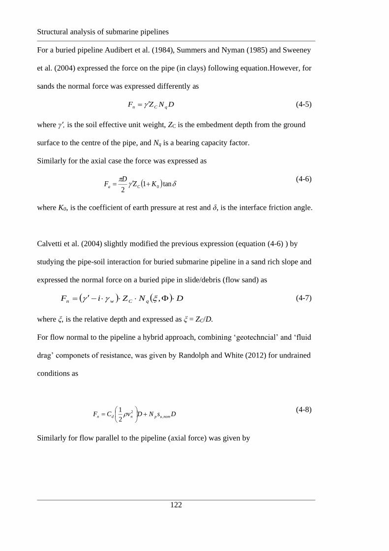
Structural analysis of submarine pipelines
122
For a buried pipeline Audibert et al. (1984), Summers and Nyman (1985) and Sweeney
et al. (2004) expressed the force on the pipe (in clays) following equation.However, for
sands the normal force was expressed differently as
DNZF qCn = (4-5)
where γʹ, is the soil effective unit weight, ZC is the embedment depth from the ground
surface to the centre of the pipe, and Nq is a bearing capacity factor.
Similarly for the axial case the force was expressed as
( )
tan12
0KZD
F Ca += (4-6)
where K0, is the coefficient of earth pressure at rest and δ, is the interface friction angle.
Calvetti et al. (2004) slightly modified the previous expression (equation (4-6) ) by
studying the pipe-soil interaction for buried submarine pipeline in a sand rich slope and
expressed the normal force on a buried pipe in slide/debris (flow sand) as
( ) ( ) DNZiF qCwn −= , (4-7)
where ξ, is the relative depth and expressed as ξ = ZC/D.
For flow normal to the pipeline a hybrid approach, combining ‘geotechncial’ and ‘fluid
drag’ componets of resistance, was given by Randolph and White (2012) for undrained
conditions as
DsNDvCF nomupndn ,
2
2
1+
= (4-8)
Similarly for flow parallel to the pipeline (axial force) was given by

Structural analysis of submarine pipelines
123
DsfF nomuaa ,= (4-9)
In these equations Cd is the drag coefficient, ρ the density of the flowing material, vn the
velocity component, Np the bearing factor, and fa friction coefficient parallel to the pipe.
su,nom is the nominal shear strength and may be expressed as
=
ref
refunomu
Dvss
.,,
/
(4-10)
where su,nom is a reference shear strength at a strain rate of γref and v is the flow velocity.
The value of fa lies between 1.2 to 1.4 for typical values of β between 0.05 and 0.15.
For slide loading of onshore buried pipelines, O'Rourke et al. (1995) established five
idealised patterns for the permanent ground deformation (PGD) shown in Figure 4-1.
Their analysis showed that, for longitudinal PGD, a block pattern results in the largest
strain in an elastic pipe. As such for the rest of this chapter the slide loading will be
idealised as a block pattern.
4.2.2 Passive loading
The passive interaction of a pipe with the seabed has been studied by many groups and
there are many reports and publications available on this topic. A summary of current
research and practice in this area is given by publications related to the SAFEBUCK JIP
and also by Randolph and White (2008a).
An alternative approach used to estimate the axial resistance, referred to as the total stress
(alpha) method, is comparable to the equivalent technique to estimate the axial active pipe
force.
For buried pipes, a similar expression was proposed by American Lifeline Alliance (2001)
(for cohesive soil) as

Structural analysis of submarine pipelines
124
DsF seabedupassive _= (4-11)
where α is a ‘adhesion’ factor which is influenced by the roughness of the surface (with
α being the relative strength of pipe-soil and soil-soil shearing), and su_seabed is the
undrained shear strength of the seabed.
For embedded pipelines Cathie et al. (2005) and Oliphant and Maconochie, (2007)
modified the expression slightly by introducing an embedment effect, with the axial
passive resistance per unit length, Fpassive expressed as
Dseabedupassive DsF = _ (4-12)
where, θD′ is the contact angle as defined in the previous chapter (see also Figure 4-3)
The alpha method for estimating the passive frictional resistance of the seabed can be
extended by integrating the seabed shear strength, su_seabed around the embedded portion
of the pipe. For conditions of zero mudline strength intercept (i.e. seabed shear strength
proportional to depth), su_seabed can be expressed as su_seabed = Rcosθ, where is the
gradient of the shear strength. Fpassive becomes
D
2/
0
Dpassive DDdcosRD2F
== (4-13)
The net axial force on a pipeline depends on the relative magnitudes of the shear strengths
of slide and seabed, and also on the pipeline embedment (expressed through D'). As the
slide material flows down the slope, the shear strength is likely to reduce significantly,
for example from 3 to 30 kPa (in situ) to 1 kPa or less as shown in Figure 4-2. By contrast
the seabed shear strength may be expected to lie in a similar range to that of the original
(in situ) submarine slide material. Modelling of the shear strength variation during the
debris flow is extremely challenging and not considered in this study. Only the effect of
the actual shear strength ratios on the pipeline structures is discussed in the next section.

Structural analysis of submarine pipelines
125
Effect of su_seabed / su_slide on the pipeline using alpha method
Following the alpha method the axial active force per unit length of the pipe (top), Fslide
due to slide loading is
( )Dslideuslide DsF −= _ (4-14)
Figure 4-3 shows the schematics of the active and passive loading on the pipe.
From the above equations a dimensionless generalised expression can be formed to
capture the effect of the ratio of su_slide / su_seabed on the ratio of the active and passive
forces, Fslide and Fpassive:
−
=
−=
D
D
slideu
seabedu
Dslideu
Dseabedu
slide
passive
s
s
Ds
Ds
F
F
_
_
_
_
)(
(4-15)
The above expression is shown as a design chart in Figure 4-4 for embedment ratios 0 <
w/D ≤ 0.5 and with various values of undrained shear strength ratios within, 0.1 < su_seabed
/ su_slide ≤ 10. From the chart it is clear that, at high su_seabed / su_slide ratios (i.e. a weak slide
relative to the seabed soil), the required embedment ratio for no net load to be transferred
to the pipeline itself is small. Also, there can be no net load on the pipeline for su_seabed /
su_slide ≤ 1.
In conventional design approaches the pipe seabed interaction is idealised by spring-slider
systems distributed at regular intervals along the length of the pipeline. A simplified
method of estimating axial soil resistance, Fpassive was proposed in BS 8010 (1993) as
WNFpassive== (4-16)
where W′, is the submerged weight of the pipe calculated as Dtpipe (pipe is density of
pipe material), and μ, is friction coefficient.

Structural analysis of submarine pipelines
126
White and Randolph (2007) modified the above expression by introducing an
enhancement factor, ζ, to account for wedging around the curved surface of the pipe as,
WNFpassive== (4-17)
The wedging factor is linked with the contact angle, θD′, as
( )DDD
D
+=
cossin
sin2
(4-18)
The factor increases to an upper limit of 1.27 for pipeline embedment of 0.5D, as shown
in the Figure 4-5.
As discussed by White and Randolph (2007) the effective stress approach (equation
(4-17)) is preferable to the total stress method, mainly because the seabed shear strength
will change due to consolidation under the pipeline weight. Therefore, the effective stress
approach is followed in this chapter for quantifying the passive resistance, Fpassive.
Effect of μWʹ/Dsu_slide on the pipeline
Using the effective stress approach for seabed friction (equation (4-17)) and alpha method
for estimating slide loading (equation (4-14)) a dimensionless generalised expression can
be formed to capture the effect of the ratio of su_slide / su_seabed on the ratio of the active
and passive forces, Fpassive and Fslide, expressed as
( ) ( )DDDD
D
slideuDslideuslide
passive
Ds
W
Ds
W
F
F
−+
=
−
=
1
cossin
sin2
)( __
(4-19)
Similar to equation (4-15) the above expression is shown as a design chart in Figure 4-6
for embedment ratios 0 < w/D ≤ 0.5 and with various values of pipe weight versus slide
shear strength ratios within, 0.1 < μWʹ/D su_slide ≤ 10. From the chart it is clear that, at
high μWʹ/D su_slide ratios (i.e. a weak slide relative to the seabed soil), the required
embedment ratio for no net load to be transferred to the pipeline itself is small. Also, there
can be no net load on the pipeline for μWʹ/D su_slide ≤ 1.

Structural analysis of submarine pipelines
127
4.3 DERIVATION OF ANALYTICAL SOLUTION
The submarine slide-pipeline-seabed interaction problem may be divided into three parts,
active slide zone, passive plastic zone and elastic zone as shown in Figure 4-7. Key loads,
displacements and frictional resistances for each zone are indicated in the schematic. The
response in each zone is solved analytically for the relevant boundary conditions in the
following sections.
4.3.2 Input parameters and dimensionless groups
The perfectly straight pipe is defined by diameter, D, wall thickness, t submerged unit
weight, Wʹ, and Young’s modulus, E, from which the axial rigidity EA can be calculated.
The slide was defined as a block pattern with length, Lslide ; to analyse the problem only
half slide length, LAB is considered here, corresponding to the ‘active slide zone’. The
length of the ‘passive plastic zone’ is LBC, beyond which point (C onwards) it is defined
as ‘elastic zone’ (Figure 4-7). The displacement at the centre of the slide, A, is uA, at the
interface of ‘active slide zone’ and ‘passive slide zone’, B, is uB and the interface of
‘passive slide zone’ and elastic zone, C is uC. The axial load generated within the pipeline
due to the slide movement along the length is defined as P. At the centre of the slide at A,
it is PA, at the interface of ‘active slide zone’ and ‘passive slide zone’, B, is PB and the
interface of ‘passive slide zone’ and elastic zone, C is PC. It is noteworthy to mention that
this idealisation assumes symmetric geometry of the slide and pipeline however, the
loading condition around the axis is asymmetric.
When a submarine landslide occurs and passes across a partially embedded pipeline with
a component of flow velocity in the longitudinal direction, the frictional resistances on
the upper portion and at the invert of the pipe are different due to variations in the physical
properties of the slide material (debris flow material) and seabed (natural fine-grained
sediment). The net (resultant) force per unit length of the pipeline is given by

Structural analysis of submarine pipelines
128
passiveslidenet FFF −= (4-20)
This may be expressed as a ratio of the passive resistance as
1−=−
=passive
slide
passive
passiveslide
passive
net
F
F
F
FF
F
F
(4-21)
The output quantities may be non-dimensionalised and expressed in terms of various
input properties. The maximum axial load, PB, may be normalised by the axial elastic
stiffness of the pipe, EA, and presented as compressive strain, = P/EA; the axial
displacement, u, may be normalised by the slide length, Lslide, as u/Lslide. These normalised
output parameters may then be expressed in terms of normalised input parameters, i.e. the
driving force, FnetLslide/EA; resisting force per diameter in passive zone, FpassiveLslide/EA;
and pipe-soil stiffness, kxLslide2/EA. Three groups can be shown to be sufficient to
determine the load and displacement of the pipe non-dimensionally.
All the input and output parameters are defined in the previous section and tabulated in
Table 4-1.
( )3211
2
1 ,,,, aaagEA
Lk
EA
LF
EA
LFg
EA
P slidexslidepassiveslidenet =
=
(4-22)
( )3212
2
2 ,,,, aaagEA
Dk
EA
LF
EA
LFg
L
u xslidepassiveslidenet
slide
=
=
(4-23)
where the normalised driving force is
EA
LFa slidenet=1
(4-24)
The resisting force per diameter in the passive zone is normalised as
EA
LFa
slidepassive=2
(4-25)

Structural analysis of submarine pipelines
129
and the pipe-soil stiffness is normalised as
EA
Lka slidex
2
3 = (4-26)
The following sections discuss the analytical solution of load, displacement and frictional
resistances on a pipe due to axial slide loading. Throughout the chapter it is assumed that
the passive resistance (equation (4-17)) continues to act (unchanged) within the active
and passive zones of the slide.
4.3.3 Elastic zone uuC
The gradient kx of the initial slope of the ‘t-z’ response of a pipeline embedded within the
seabed was considered in chapter 3, focusing in particular on conditions where the seabed
shear modulus G varies proportionally with depth z according to G = mz. An approximate
closed form solution for kx was developed by considering the deformation of a vertical
(or radial) circular slice comprising a short element of pipe and the surrounding soil.
The axial elastic stiffness of a pipeline on the seabed is then given by
Dmu
Fk x
== (4-27)
where m is the gradient of the shear modulus and D′ is the contact width, which can be
expressed as D′ = Dsin D'.
The axial load generated in the pipe due to the presence of frictional resistance of the
seabed is
Fdx
dP−=
(4-28)
The compressive strain, εx, of the pipeline (assumed elastic) is written in terms of the load,
P, transmitted by the pipe at any length x,
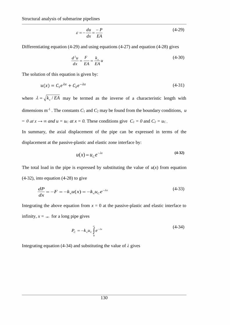
Structural analysis of submarine pipelines
130
EA
P
dx
du −=−=
(4-29)
Differentiating equation (4-29) and using equations (4-27) and equation (4-28) gives
uEA
k
EA
F
dx
ud x==2
(4-30)
The solution of this equation is given by:
𝑢(𝑥) = 𝐶1𝑒𝜆𝑥 + 𝐶2𝑒−𝜆𝑥 (4-31)
where EAkx /= may be termed as the inverse of a characteristic length with
dimensions m-1 . The constants C1 and C2 may be found from the boundary conditions, u
= 0 at x → ∞ and u = uC at x = 0. These conditions give C1 = 0 and C2 = uC .
In summary, the axial displacement of the pipe can be expressed in terms of the
displacement at the passive-plastic and elastic zone interface by:
x
C euxu −=)( (4-32)
The total load in the pipe is expressed by substituting the value of u(x) from equation
(4-32), into equation (4-28) to give
x
Cxx eukxukFdx
dP −−=−=−= )( (4-33)
Integrating the above equation from x = 0 at the passive-plastic and elastic interface to
infinity, x = for a long pipe gives
−−=0
x
CxC eukP (4-34)
Integrating equation (4-34) and substituting the value of λ gives

Structural analysis of submarine pipelines
131
Cx
x
CxC uEAk
EA
k
ukP ==
(4-35)
In non-dimensional form, this may be written as
slide
C
slide
CslidexC
L
ua
L
u
EA
Lk
EA
P3
2
==
(4-36)
Since point C (Figure 4-7) represents the interface between passive plastic and elastic
zones, using equation (4-27) the elastic slip uC-slip may be expressed as
x
passive
slipCk
Fu =− hence
3
2
2 a
a
Lk
EA
EA
LF
L
u
slidex
slidepassive
slide
slipC==
−
(4-37)
Therefore, using equation (4-35) and (4-37) the elastic load in the long pipe is given as
x
passiveCk
EAFP =max,
hence 3
2max,
a
a
EA
PC=
(4-38)
4.3.4 Passive slide zone CB uuu
In general, there will be a passive plastic zone between the active slide zone and the elastic
zone, where slip occurs between the seabed and the pipe and the resistance force per unit
length is Fpassive. The governing equations of the plastic zone are similar to those for the
elastic zone. The compatibility equation for horizontal equilibrium is:
passiveFdx
dP−=
(4-39)
Integrating the above equation within B-C (Figure 4-7) gives
−=
C
B
passive
C
B
dxFdP (4-40)

Structural analysis of submarine pipelines
132
The axial load in the passive slide zone is expressed by integrating equation (4-40) as
BCpassiveCB LFPP =− (4-41)
Therefore, the length of passive zone, LBC is
passive
CBBC
F
PPL
−= hence
2
1
aEA
P
EA
P
L
L CB
slide
BC
−=
(4-42)
When the passive zone LBC = 0, point B coincides with point C leading to PB = PC. In
general, though, we may write PB ≥ PC and LBC ≥ 0.
The axial deformation can be approximated by a compatibility equation for strain, εx
( )EA
xP
dx
du−=
(4-43)
where P is the varying load between B and C. Integrating the above equation gives the
compression in the passive-plastic zone as
−=
C
B
C
B
dxxPEA
du )(1
(4-44)
where B is the boundary point at the active-passive intersection, C is the boundary point
at the elastic zone and P(x) is the linearly varying load between B and C.
Now integrating equation (4-44) gives the compression in the passive-plastic zone:
( )BC
CB
CB LEA
PPuu
2
+=−
(4-45)
Therefore, using equation (4-42), the displacement, uB at the active-passive intersection
can be expressed as

Structural analysis of submarine pipelines
133
passive
CB
CBEAF
PPuu
2
22 −+= hence
𝑢𝐵
𝐿𝑠𝑙𝑖𝑑𝑒=
𝑢𝐶
𝐿𝑠𝑙𝑖𝑑𝑒+
1
2
(𝑃𝐵2−𝑃𝐶
2)
𝐸𝐴2
𝐸𝐴
𝐹𝑝𝑎𝑠𝑠𝑖𝑣𝑒𝐿𝑠𝑙𝑖𝑑𝑒
(4-46)
For a small active slide load (or strong passive resistance), the elastic limit of uC-slip may
not be reached, in which case LBC = 0, PB = PC and uB = uC.
4.3.5 Active slide zone BA uuu
In the active zone the interaction between the pipe and the soil is assumed to be plastic.
The displacement is taken as uA at the centre (x = 0) of the slide from the symmetry. The
equation for horizontal equilibrium is
netFdx
dP−=
(4-47)
where Fnet is given by equation (4-20). Integrating equation (4-47) within the active
slide zone, A-B, gives
−=
B
A
net
B
A
dxFdP (4-48)
The axial load can be expressed by integrating equation (4-48)
2
slidenetABnetBA
LFLFPP −=−=−
(4-49)
where LAB is the half slide length, Lslide/2. Assuming the axial load at the centre of the
slide is zero, PA = 0, from symmetry, gives.

Structural analysis of submarine pipelines
134
2
slidenet
B
LFP = hence
22
1 1a
EA
LF
EA
P slidenetB == (4-50)
Note that PB represents the largest axial force generated in the pipeline, and hence the
maximum compressive strain in the pipe is max = a1/2.
Similar to equation (4-43) the axial deformation can be calculated using a compatibility
equation for strain, εx
( )EA
xP
dx
dux −=−=
(4-51)
Integrating this, allowing for the linear variation of P between PA (= 0) and PB gives
−=
A
B
A
B
dxxPEA
du )(1
(4-52)
Therefore, using equation (4-50) the axial deformation within the slide zone is
EA
LF
EA
LPuu slidenetslideB
BA84
2
==− hence 8
1a
L
u
L
u
slide
B
slide
A += (4-53)
4.3.6 Summary of solution
For convenience the main expressions are summarized here in non-dimensional form.
The key loads may be expressed as
===
3
211 ,2
;2
;0a
aaMin
EA
Pa
EA
P
EA
P CBA (4-54)
The length of the (plastic) passive zone is given by
−=
32
1 1
2 , 0
aa
aMax
L
L
slide
BC (4-55)
The displacements at key points are
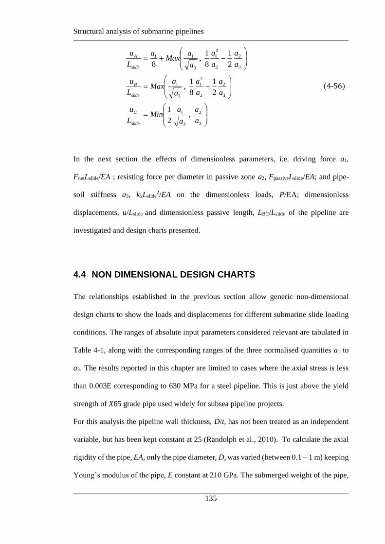
Structural analysis of submarine pipelines
135
=
−=
−+=
3
2
3
1
3
2
2
2
1
3
1
3
2
2
2
1
3
11
, 2
1
2
1
8
1 ,
2
1
8
1 ,
8
a
a
a
aMin
L
u
a
a
a
a
a
aMax
L
u
a
a
a
a
a
aMax
a
L
u
slide
C
slide
B
slide
A
(4-56)
In the next section the effects of dimensionless parameters, i.e. driving force a1,
FnetLslide/EA ; resisting force per diameter in passive zone a2, FpassiveLslide/EA; and pipe-
soil stiffness a3, kxLslide2/EA on the dimensionless loads, P/EA; dimensionless
displacements, u/Lslide and dimensionless passive length, LBC/Lslide of the pipeline are
investigated and design charts presented.
4.4 NON DIMENSIONAL DESIGN CHARTS
The relationships established in the previous section allow generic non-dimensional
design charts to show the loads and displacements for different submarine slide loading
conditions. The ranges of absolute input parameters considered relevant are tabulated in
Table 4-1, along with the corresponding ranges of the three normalised quantities a1 to
a3. The results reported in this chapter are limited to cases where the axial stress is less
than 0.003E corresponding to 630 MPa for a steel pipeline. This is just above the yield
strength of X65 grade pipe used widely for subsea pipeline projects.
For this analysis the pipeline wall thickness, D/t, has not been treated as an independent
variable, but has been kept constant at 25 (Randolph et al., 2010). To calculate the axial
rigidity of the pipe, EA, only the pipe diameter, D, was varied (between 0.1 – 1 m) keeping
Young’s modulus of the pipe, E constant at 210 GPa. The submerged weight of the pipe,

Structural analysis of submarine pipelines
136
W, was calculated as Dtpipe, with the density of the pipe material, pipe kept constant at
7900 kg/m3. A pipe embedment ratio of w/D = 0.5 and coefficient of friction, = 0.3
were adopted. The soil shear modulus gradient, m, was varied between 0.1-10 MPa/m.
Slide lengths, Lslide, ranging between 50 and 1000 m were considered along with shear
strength, su_slide , varying from 0.1 – 10 kPa. With these raw input data, relatively wide
ranges of non-dimensional input parameters (see Table 4-1) were estimated, from which
design charts for the various non-dimensional output parameters were drawn.
The non-dimensional slide force, a1, is taken as the primary influence on the non-
dimensional loads (PB/EA, PC/EA), non-dimensional displacements (uA/Lslide, uB/Lslide and
uC/Lslide) and non-dimensional passive length LBC/Lslide. The relationships are plotted for
different values of the secondary influence, the non-dimensional passive resistance, a2.
Then different charts are shown for different values of pipe soil elastic stiffness
parameter, a3.
4.4.1 Effect of slide force on pipe loading
Figure 4-8, Figure 4-9 and Figure 4-10 respectively show the variations of PB/EA and PC/EA
as functions of non-dimensional slide force, for different values of passive resistance, a2 =
0.00001 to 0.0001, for three values of pipe-soil elastic parameter, a3 = 0.01, 3 and 1000. The
maximum non-dimensional load, PB/EA is directly proportional to the non-dimensional slide
force, a1, while the load at the transition from elastic to plastic soil resistance, PC/EA, is initially
proportional to a1 but then is limited (equation (4-54)). The limit is reached for most relevant
values of the slide force.
4.4.2 Effect of slide force on passive length
Figure 4-11, Figure 4-12, and Figure 4-13 show the corresponding variations of non-
dimensional passive length with dimensionless slide force for different values of passive
resistance, a2 = 0.00001 to 0.0001, and for pipe-soil elastic parameter, a3 = 0.01, 3 and 1000

Structural analysis of submarine pipelines
137
respectively. The length of the passive zone increases linearly with increasing slide force, with
the gradient inversely proportional to the passive resistance, a2.
4.4.3 Effect of slide force on displacements
The peak axial dimensionless axial displacement, uA/Lslide, increases with increasing slide force.
Figure 4-14, Figure 4-15, and Figure 4-16 show the variation of dimensionless displacement
with slide force for various resistances, a2 = 0.00001 to 0.0001 and for a3 = 0.01, 3 and 1000. The
axial displacement increases with increasing slide force, but at a rate that decreases with
increasing passive resistance. The elastic stiffness parameter, a3, has essentially negligible
influence.
Similarly, the normalised slide displacement, uB/Lslide, increases with increasing slide force.
Figure 4-17, Figure 4-18, and Figure 4-19 show the variation of dimensionless displacement
with slide force. Increasing passive resistance, a2, reduces the displacements in the slide and
passive zones. The values of the dimensionless peak displacements, uA/Lslide, are slightly higher (
1%) than the dimensionless slide displacements, uB/Lslide.
The normalised elastic displacements increase with increasing slide loading until it reaches the
limiting value at which slip occurs, as shown in Figure 4-20, Figure 4-21and Figure 4-22. The
slip displacement increases proportionally with resistance in the passive zone, and inversely with
the value of a3.
4.5 DISCUSSION
To compare the individual dimensionless displacements uA/Lslide, uB/Lslide and uC/Lslide, these are
plotted together on Figure 4-23 for a2 = 0.00001 and 0.0001 and a3=0.01. The peak and slide
displacements match closely for different values of a2. However, the values of elastic
displacement are much less than the peak and slide displacements. It is also useful to compare the
elastic load, Pc/EA, for different values of pipe-soil elastic stiffness, keeping a2 constant. Figure
4-24 shows the normalised elastic load as a function of the slide force for three different values
of a3 = 0.01, 3 and 1000, keeping a2 = 0.0001. For a normalised slide force of 0.006, Pc/EA =

Structural analysis of submarine pipelines
138
0.001 for a3 = 0.01 and decreases significantly for a3 = 1000 to a value of Pc/EA = 3.2x10⁻⁶. Figure
4-25 shows the effect of the pipe-soil elastic parameter on the passive length. It is evident that
the pipe-soil elastic stiffness has negligible effect on the passive length. Figure 4-26 shows a
similar observation of insignificant effect of the pipe-soil elastic stiffness on the peak
displacement. Figure 4-27 shows a comparison of normalised elastic displacements as a function
of slide load for three different values of a3 = 0.01, 3 and 1000, keeping a2 = 0.0001. For a
normalised slide load of 0.006, uc/Lslide = 0.0000001for a3 = 1000 and increases significantly to a
value of uc/Lslide = 0.01 for a a3 = 0.01.
Normalised displacements are plotted against the normalised slide length, Lslide/D, for the whole
range of data in Figure 4-28. For an embedment ratio of w/D = 0.5 and coefficient of friction, μ
= 0.3, the normalised peak and slide displacements increase with increasing Lslide/D, whereas the
normalised elastic displacement decreases with increasing Lslide/D ratio. Normalised loads, P/EA
are also plotted against the normalised slide length, Lslide/D or the whole range of data in Figure
4-29 to show the effect of slide length. For an embedment ratio of w/D = 0.5 and coefficient of
friction, μ = 0.3, the peak loads increase with increasing Lslide/D. However, for shorter slide
lengths, elastic and peak loads merge (since no plastic zone) while for longer slides the elastic
loads are much lower than the peak loads.
In the next section example cases are studied to integrate all the analytical solutions together.
Numerical results are also compared with the analytical results.
4.5.1 Example cases
Example cases were studied to explore the variation of load and displacement behaviour
along the length of the pipeline. For this analysis the adopted pipeline properties were, D
= 1 m, D/t = 25, E = 210 GPa, Wʹ = 7.8 kN/m, μ = 0.3 and embedment ratio, w/D = 0.5.
Three different slide lengths with Lslide = 100, 300 and 500 m were considered, taking the
shear strength of the slide material as su_slide = 10 kPa. The corresponding non-dimensional
parameters are tabulated in Table 4-2.

Structural analysis of submarine pipelines
139
The axial compressive strain, P/EA = ε (%), the dimensionless axial displacement, u/Lslide
and frictional resistance distribution along the length of the pipeline are presented here.
Figure 4-30 shows the distribution of compressive strain along the pipeline for Lslide/D =
100. In the active slide zone the axial load increases from zero (at the centre of the slide)
with a positive slope equal to the net resistance force, Fnet, until reaching a maximum
value at the edge of the slide. In the passive zone the axial load decreases linearly, thereby
decreasing the compressive strain, with a negative slope equal to the passive resistance
of seabed, Fpassive. In the elastic zone the distribution of strain decreases exponentially
towards zero far from the slide.
The dimensionless displacement profile of the pipe along its length is shown in Figure
4-31. The displacement is maximum at the centre of the active slide zone, and decreases
in the passive slide and elastic zones. In the ‘elastic’ zone the displacements decay
exponentially with distance from the slide.
The variation of normalised frictional resistance along the length of the pipe is plotted in
Figure 4-32. In the active zone applied frictional resistance force per unit length, Fnet is
very high and plotted as a positive quantity, whereas the values of passive resistance force,
Fpassive in the passive slide zone is comparatively lower and plotted as a negative quantity.
In the ‘elastic’ zone the passive resistance force of the seabed decays exponentially with
distance from the slide.
In order to show the effect of different slide lengths on the axial strain, displacement and
frictional resistance distribution along the length, a set of three cases were undertaken.
These cases examine the effects of slide loading for Lslide/D = 100, 300 and 500 (see Table
4-2). Figure 4-33, Figure 4-34 and Figure 4-35 show the variation of compressive strains,
axial displacements and frictional resistance forces along the pipe respectively. The
maximum values of compressive strains, axial displacements and frictional resistance

Structural analysis of submarine pipelines
140
forces are directly proportional to the slide length when other conditions are kept constant.
Thus, for a slide with length of 500 m the value of maximum strain is exactly five times
higher than the value for a 100 m long slide.
4.5.2 Numerical verification
Numerical analysis provides an alternate general method to analyse the effect of slide
impact on a seabed pipeline (Randolph et al., 2010). The finite-element-analysis (FEA)
software ABAQUS, (Dassault Systèmes, 2007) was used to verify the analytical solution.
Figure 4-36 illustrates the schematic diagram and FE mesh used for this. The modelling
was carried out for the passive and elastic zones of the pipe, starting from B and
approximating an infinitely long straight pipe consistent with the analytical solution by
taking L∞ = 5000 m. This was the only limitation of the FEA model. The boundaries of
the pipe were left free to represent the conditions at B and at far distance from the slide.
The slide loading was assumed to increase monotonically, with a concentrated
compressive load applied to the pipe at B. The seabed was modelled with springs, with
the nonlinear behaviour of seabed resistance incorporated using a bi-linear load-
displacement behaviour (Summers & Nyman, 1985). The pipe was modelled with
Timoshenko beam elements (ABAQUS code B21), which model linear elastic transverse
shear behaviour (Randolph et al., 2010).
Figure 4-37 shows the distribution of normalised axial displacements for the three
different slide lengths considered in Table 4-2. The FE results are shown by solid triangles,
while the analytical solutions are represented by solid lines. The analytical solutions start
from coordinate x/D = 0, while the FE solutions start from the passive zones (point B) of
the corresponding cases. Overall analytical and FE results are in good agreement.

Structural analysis of submarine pipelines
141
4.6 SENSITIVITY OF BUCKLING
A detailed investigation of the sensitivity of the pipeline to buckling under axial
compressive load is provided in the next chapter, but a brief discussion is relevant here.
In the above analytical solutions, the buckling response of the pipeline was ignored.
Analytical solutions for the critical buckling load for a straight pipe on a rigid seabed was
investigated by several researchers including Hobbs (1981), Maltby & Calladine (1995)
and Tran & Taylor (1996). Recently the SAFEBUCK JIP has introduced new analytical
solution for three modes of buckling. Also, Peek (2009) corrected the lateral buckling
solutions previously published. Therefore, in this section the critical buckling load was
estimated using the solution proposed by Peek (2009). The maximum axial load attained
in each case of slide loading was compared with the buckling initiation load to estimate
the susceptibility to buckling. The post-buckling load was estimated for a pipe of unit
weight, W, with axial and bending stiffnesses of EA and EI respectively, resting on a flat
seabed with lateral friction coefficient, L = 0.6, as:
4/122183076.8 EIqEAP bucklepost =− (4-57)
where q = WL. The minimum axial force prior to buckling for which a buckled solution
is possible was obtained as:
( ) bucklepostbuckle PP −= 3/4 (4-58)
Here only lateral buckling was considered and estimated by equation (4-58). The ratios of
peak load versus buckling load, PB/Pbuckle are plotted against the normalised slide length, Lslide/D
(for μ/μL = 1) in the same graph (Figure 4-38) for the whole range of data (Table 4-1). To see
the effect of slide loading, cases with Fnet/Fpassive = 1.07 – 40.42 are adopted here. Increasing slide
length and Fnet/Fpassive ratio increases the vulnerability of lateral buckling of the pipeline.
Structural analysis of submarine pipelines
142
4.7 CONCLUSIONS
An analytical solution was presented here for axial submarine slide loading of a straight
on-bottom pipeline. Non-dimensional expressions for axial load distribution and axial
displacement along the length of the pipeline were derived analytically.
It was shown that the non-dimensional axial loads and axial displacements depend on
three non-dimensional input parameters, i.e. the driving force in the slide zone, seabed
resisting force in passive zone, and pipe-soil stiffness. Non-dimensional design charts
were presented to show the effect of individual input parameters on axial loads and axial
displacements. The maximum axial load in the pipe is directly proportional to the slide
force, while the load at the transition from elastic to plastic soil resistance is initially
proportional to the slide force but then becomes limited. The limit is reached for most
relevant values of the slide force. The length of the passive zone was also derived non-
dimensionally and shown to increase linearly with increasing slide force, with the
gradient inversely proportional to the passive resistance. It was also shown that the axial
displacement increases with increasing slide force, but at a rate that decreases with
increasing passive resistance. The elastic stiffness parameter has essentially negligible
influence.
Numerical FE analysis was also carried out to verify the analytical model. Analytical and
numerical solutions were shown to match with close agreement. The buckling was
ignored in the analytical model. However, the existing classical theory of buckling was
linked to the output of the analytical model to show the vulnerability of the pipelines
towards buckling in case of various slide loading conditions. On bottom submarine
pipelines are more susceptible to lateral buckling when impacted axially by stronger and
longer slides.
Structural analysis of submarine pipelines
143
The presented analytical framework can be used by industry practitioners to estimate the
maximum axial slide loading for a straight pipe resting on seabed. At the same time load
distribution and axial movement of the pipe along the length of the pipeline can also be
estimated.

Structural analysis of submarine pipelines
144
Table 4-1: Summary of range of input and output parameters
Range of Raw Input parameter Symbol Units
Pipeline diameter, D 0.1 - 1 m
Elastic modulus of Pipeline steel, E 210 GPa
Submerged pipe weight, W 7.8 kN/m
Length of slide loading on pipeline,
Lslide
50 - 1000 m
Shear strength of slide, su_slide 0.1 – 10 kPa
Coefficient of axial friction, 0.3
Coefficient of lateral friction, L 0.3
Shear modulus gradient, m 0.1 - 10 MPa/m
Embedment ratio, w/D 0.5
Range of Calculated Input
parameter
Passive seabed frictional
resistance force, Fpassive
0.037 – 3.7 kN/m
Active slide force on
pipeline, Fslide
0.047 – 15.7 kN/m
Net slide force on pipeline,
Fnet
0.119 - 11.9 kN/m
Pipe-soil elastic axial
stiffness, kx
10 – 10,000 kPa
Axial rigidity of pipe, EA 253 - 253333 MN
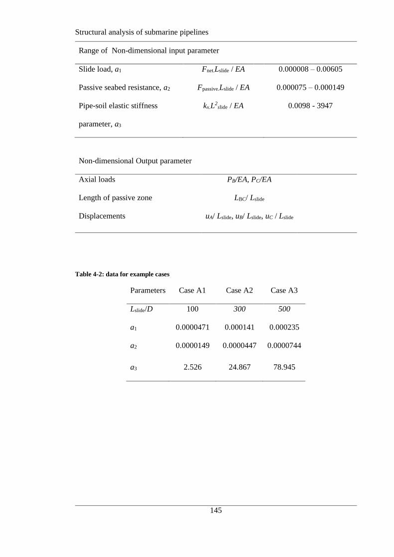
Structural analysis of submarine pipelines
145
Range of Non-dimensional input parameter
Slide load, a1 Fnet.Lslide / EA 0.000008 – 0.00605
Passive seabed resistance, a2 Fpassive.Lslide / EA 0.000075 – 0.000149
Pipe-soil elastic stiffness
parameter, a3
kx.L2
slide / EA 0.0098 - 3947
Non-dimensional Output parameter
Axial loads PB/EA, PC/EA
Length of passive zone LBC/ Lslide
Displacements uA/ Lslide, uB/ Lslide, uC / Lslide
Table 4-2: data for example cases
Parameters Case A1 Case A2 Case A3
Lslide/D 100 300 500
a1 0.0000471 0.000141 0.000235
a2 0.0000149 0.0000447 0.0000744
a3 2.526 24.867 78.945

Structural analysis of submarine pipelines
146
References:
American Lifeline Alliance (2001). “Guideline for the Design of Buried Steel Pipe.”
ASCE, USA.
Audibert, J. M. E., & Nyman, K. J. (1977). Soil restraint against horizontal motion of
pipes. Journal of Geotechnical Engineering, ASCE, Vol. 114, No. 6, GT10,
1119-1142.
Bea, R. G. and Aurora, R. (1982). “Design of pipelines in mudslide areas.” Proc.,
Offshore Technology Conference, Houston, 401-414.
Bruschi, R., Bughi, S., Spinazze,M., Torselletti, E., and Vitali, L. (2006). “Impact of
debris flows and turbidity currents on seafloor structures.” Norw. J. Geol., 86,
317-337.
BS 8010 (1993). “Code of practice for Pipelines, Part3: Pipelines subsea: design,
construction and installation.” BSI, London.
Dassault Systèmes Simulia. (2007). ABAQUS analysis users’ manual, Providence, RI,
USA.
Demars, K. R. (1978). “Design of marine pipelines for areas of unstable sediment.”
Transp. Eng. J., 104(1), 109-112.
Georgiadis, M. (1991). “Landslide drag forces on pipelines.” Soils Found., 31(1), 156-
161.
Hobbs, R. E. (1984). “In-service buckling of heated pipelines.” J. Transp. Eng., 110(2),
175-189.
Kishida, H., and Uesugi, M. (1987). “Tests of interface between sand and steel in the
simple

Structural analysis of submarine pipelines
147
shear apparatus.” Géotechnique, 37 (1), 46-52.
Kvalstad, T. J., Nadim, F., and Harbitz, C. B. (2001). “Deepwater geohazards:
geotechnical concerns and solutions.” Proc., Offshore Technology Conference,
Houston, Paper OTC 12958.
Maltby, T. C., and Calladine, C. R. (1995). “An investigation into upheaval buckling of
buried pipelines-II. Theory and analysis of experimental observations.” Int. J.
Mech. Sci., 37(9), 965-983.
Oliphant, J., and Macanochie, A. (2007). “The axial resistance of buried and unburied
pipelines.” Proc., 6th International Offshore Site Investigation and Geotechnics
Conference: Confronting New Challenges and Sharing Knowledge, London.
O’Rourke, M.J., Liu, X.J., and Flores-Berrones, R. (1995). “Steel pipe wrinkling due to
longitudinal permanent ground deformations.” J. Transport. Eng., 121(5), 443-
451.
Peek, R. (2009). “Correction to the Infinite Mode for Lateral Buckling of Pipeline.” J.
Transp. Eng., 135(9), 668-669.
Ramberg, W., and Osgood, W. (1943). “Description of stress-strain curves by three
parameters.” Technical Notes, No. 902, National Advisory Committee for
Aeronautics, 28p.
Randolph, M. F. (1977). “A Theoretical Study of the Performance of Piles.” Ph.D.
dissertation, Dept of Civil Engineering, Cambridge University, England.
Randolph, M. F., and White, D. J. (2008). “Offshore Foundation Design – A Moving
Target.” Proc., BGA International Conference on Foundations, Dundee, HIS
BRE Press, London, 27-59.

Structural analysis of submarine pipelines
148
Randolph, M. F., Seo, D., and White, D. J. (2010). “Parametric solution of slide impact
on pipelines.” J Geotech Geoenviron Eng., 136(7), 940-949.
SAFEBUCK (2008). “Safe design of pipelines with lateral buckling – design guideline,
SAFEBUCK JIP Report.” BR02050/SAFEBUCK/C Phase II, December 2008.
Summers, P. B., and Nyman, D. J. (1985). “An approximate procedure for assessing the
effects of mudslides on offshore pipelines.” J. Energy Resource Tech., 107(4), 426-
432.
Swanson, R. C., and Jones, W. T. (1982). “Mudslide effects on offshore pipelines.”
Transp. Engrg. J., 108(6), 585-600.
Sweeney, M., Gasca, A. H., Garcia Lopez, M., and Palmer, A. C. (2004). “Pipelines and
landslide in rugged terrain: A database, historic risk and pipeline vulnerability.”
Proc., Int. Conf. on Terrain and Geohazard Challenges Facing Oil and Gas
Pipelines, Thomas Telford, London, 647-659.
Taylor, N. and Tran, V. (1996). “Experimental and theoretical studies in subsea pipeline
buckling.” Mar. Struct., 9, 211-257.
White, D. J., and Randolph, M. F. (2007). “Seabed characterisation and models for
pipeline-soil interaction.” Int. J. Offshore Polar Eng, 17(3), 193-204.
Zakeri, A. (2009). “Review of state-of-art: Drag force on submarine pipelines and piles
caused by landslide or debris flow impact.” J. Offshore Mech. Arct. Eng., 131(1), ,
014001.

Structural analysis of submarine pipelines
149
Figures:
Figure 4-1: Idealized pattern for longitudinal PGD. a) Block pattern b) Ramp pattern c)
Ridge pattern d) Ramp-ridge pattern e) Asymmetric ridge pattern ( O’Rourke et al.
1995)

Structural analysis of submarine pipelines
150
Soil strength distribution along the slide length
Slope failure
Debris flow Turbidity
current
Vert
ical sc
ale
3-30 kPa 10 kPa 0.01-0.1 kPa1 kPa
Pipe position
Soil strength distribution along the slide length
Slope failure
Debris flow Turbidity
current
Vert
ical sc
ale
3-30 kPa 10 kPa 0.01-0.1 kPa1 kPa
Pipe position
Figure 4-2: Schematic diagram of submarine slide stages with the shear strength
distribution along the slide length. (White et al. 2008, MERIWA project report no. M395)
Wʹ
θDʹ
θDʹ
Dʹ
w
D
Fslide=αsu_seabedD(π-θDʹ)
Fpassive=μζWʹ
Slide along the
length of pipe
Seabed
Figure 4-3: Schematic of frictional resistances on an embedded pipe during axial slide
loading
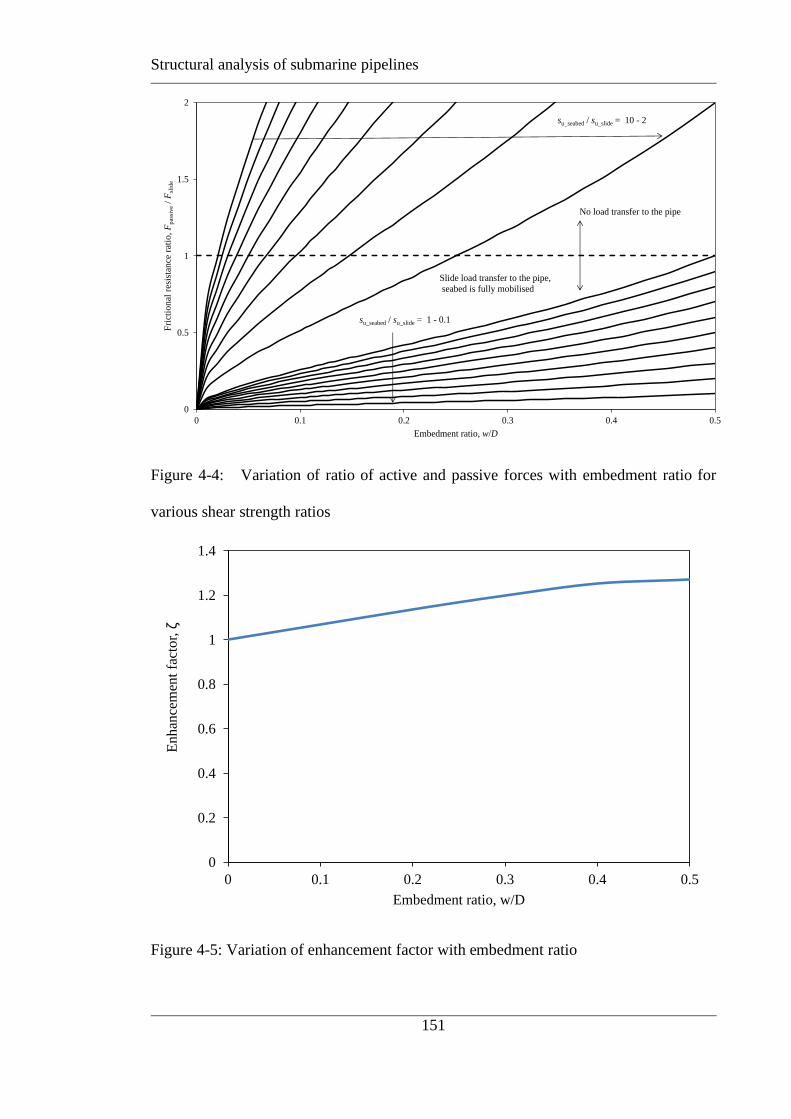
Structural analysis of submarine pipelines
151
0
0.5
1
1.5
2
0 0.1 0.2 0.3 0.4 0.5
Fri
ctio
nal
res
ista
nce
rat
io,
Fp
ass
ive
/ F
slid
e
Embedment ratio, w/D
su_seabed / su_slide = 10 - 2
su_seabed / su_slide = 1 - 0.1
No load transfer to the pipe
Slide load transfer to the pipe,
seabed is fully mobilised
Figure 4-4: Variation of ratio of active and passive forces with embedment ratio for
various shear strength ratios
0
0.2
0.4
0.6
0.8
1
1.2
1.4
0 0.1 0.2 0.3 0.4 0.5
En
han
cem
ent
fact
or,
ζ
Embedment ratio, w/D
Figure 4-5: Variation of enhancement factor with embedment ratio

Structural analysis of submarine pipelines
152
0
1
2
3
4
0 0.1 0.2 0.3 0.4 0.5
Fri
ctio
nal
res
ista
nce
rat
io,
Fp
assi
ve
/ F
slid
e
Embedment ratio, w/D
μW' /Dsu_slide = 10 - 2
No load transfer
to the pipe
Slide load transfer to the pipe,
seabed is fully mobilised
μW' /Dsu_slide = 1-0.1
Figure 4-6: Variation of ratio of passive and active forces with embedment ratio for
various μWʹ/Dsu_seabed ratios
Figure 4-7: Idealisation of axial slide pipeline interaction

Structural analysis of submarine pipelines
153
0
0.001
0.002
0.003
0 0.001 0.002 0.003 0.004 0.005 0.006
Dim
ensi
on
less
ax
ial
load
, P
/EA
Dimensionless slide force, FnetLslide/EA
a3 = 0.01
Pc: a2= 0.0001 - 0.00001
PB
Figure 4-8: Effect of dimensionless slide force on axial loads of the pipe for a3 = 0.01
0
0.0001
0.0002
0.0003
0 0.0002 0.0004 0.0006
Dim
ensi
onle
ss ax
ial
load
, P
/EA
Dimensionless slide force, FnetLslide/EA
a3 = 3
Pc: a2= 0.0001 - 0.00001
PB
Figure 4-9: Effect of dimensionless slide force on axial loads of the pipe for a3 = 3

Structural analysis of submarine pipelines
154
0
0.00005
0.0001
0.00015
0.0002
0 0.0001 0.0002 0.0003 0.0004
Dim
ensi
on
less
ax
ial
load
, P
/EA
Dimensionless slide force, FnetLslide/EA
a3 = 1000
PB
Pc: a2= 0.0001 - 0.00001
Figure 4-10: Effect of dimensionless slide force on axial loads of the pipe for a3 = 1000
0
100
200
300
0 0.001 0.002 0.003 0.004 0.005 0.006
Dim
ensi
onle
ss p
assi
ve
length
, L
BC/L
slid
e
Non-dimensional slide force, FnetLslide/EA
a3 = 0.01
a2= 0.00001- 0.0001
Figure 4-11: Effect of dimensionless slide force on passive zone length for a3 = 0.01

Structural analysis of submarine pipelines
155
0
40
80
120
160
200
240
280
320
0 0.001 0.002 0.003 0.004 0.005 0.006
Dim
ensi
on
less
pas
siv
e le
ngth
, L
BC/L
slid
e
Non-dimensional slide force, FnetLslide/EA
a3 =3
a2= 0.00001- 0.0001
Figure 4-12: Effect of dimensionless slide force on passive zone length for a3 = 3
0
40
80
120
160
200
240
280
320
0 0.001 0.002 0.003 0.004 0.005 0.006
Dim
ensi
on
less
pas
siv
e le
ngth
, L
BC/L
slid
e
Non-dimensional slide force, FnetLslide/EA
a3 =1000
a2= 0.00001- 0.0001
Figure 4-13: Effect of dimensionless slide force on passive zone length for a3 = 1000
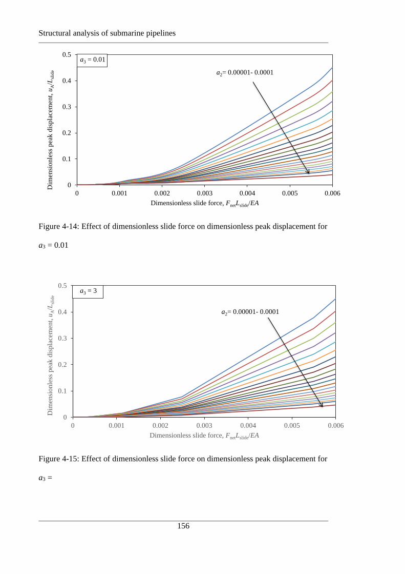
Structural analysis of submarine pipelines
156
0
0.1
0.2
0.3
0.4
0.5
0 0.001 0.002 0.003 0.004 0.005 0.006
Dim
ensi
onle
ss p
eak d
ispla
cem
ent,
uA/L
slid
e
Dimensionless slide force, FnetLslide/EA
a3 = 0.01
a2= 0.00001- 0.0001
Figure 4-14: Effect of dimensionless slide force on dimensionless peak displacement for
a3 = 0.01
0
0.1
0.2
0.3
0.4
0.5
0 0.001 0.002 0.003 0.004 0.005 0.006
Dim
ensi
on
less
pea
k d
isp
lace
men
t, u
A/L
slid
e
Dimensionless slide force, FnetLslide/EA
a3 = 3
a2= 0.00001- 0.0001
Figure 4-15: Effect of dimensionless slide force on dimensionless peak displacement for
a3 =

Structural analysis of submarine pipelines
157
0
0.1
0.2
0.3
0.4
0.5
0 0.001 0.002 0.003 0.004 0.005 0.006
Dim
ensi
onle
ss p
eak d
ispla
cem
ent,
uA/L
slid
e
Dimensionless slide force, FnetLslide/EA
a3 = 1000
a2= 0.00001- 0.0001
Figure 4-16: Effect of dimensionless slide force on dimensionless peak displacement for
a3 = 1000
0
0.1
0.2
0.3
0.4
0.5
0 0.001 0.002 0.003 0.004 0.005 0.006
Dim
ensi
on
less
sli
de
dis
pla
cem
ent,
uB/L
slid
e
Dimensionless slide force, FnetLslide/EA
a3 = 0.01
a2= 0.00001- 0.0001
Figure 4-17: Effect of dimensionless slide force on dimensionless slide displacement for
a3 = 0.01

Structural analysis of submarine pipelines
158
0
0.1
0.2
0.3
0.4
0.5
0 0.001 0.002 0.003 0.004 0.005 0.006
Dim
ensi
on
less
sli
de
dis
pla
cem
ent,
uB/L
slid
e
Dimensionless slide force, FnetLslide/EA
a3 = 3
a2= 0.00001- 0.0001
Figure 4-18: Effect of dimensionless slide force on dimensionless slide displacement for
a3 = 3
0
0.1
0.2
0.3
0.4
0.5
0 0.001 0.002 0.003 0.004 0.005 0.006
Dim
ensi
on
less
sli
de
dis
pla
cem
ent,
uB/L
slid
e
Dimensionless slide force, FnetLslide/EA
a3 = 1000
a2= 0.00001 - 0.0001
Figure 4-19: Effect of dimensionless slide force on dimensionless slide displacement for
a3 = 1000

Structural analysis of submarine pipelines
159
0
0.004
0.008
0.012
0 0.001 0.002 0.003 0.004 0.005 0.006
Dim
ensi
onle
ss e
last
ic d
ispla
cem
ent,
uC/L
slid
e
Dimensionless slide force, FnetLslide/EA
a3 = 0.01 a2= 0.0001 - 0.00001
Figure 4-20: Effect of dimensionless slide force on dimensionless elastic displacement
for a3 = 0.01
0
0.00001
0.00002
0.00003
0.00004
0 0.001 0.002 0.003 0.004 0.005 0.006
Dim
ensi
on
less
ela
stic
dis
pla
cem
ent,
uC/L
slid
e
Dimensionless slide force, FnetLslide/EA
a3 = 3 a2= 0.0001 - 0.00001
Figure 4-21: Effect of dimensionless slide force on dimensionless elastic displacement
for a3 = 3

Structural analysis of submarine pipelines
160
0
4E-08
8E-08
1.2E-07
0 0.001 0.002 0.003 0.004 0.005 0.006
Dim
ensi
on
less
ela
stic
dis
pla
cem
ent,
uC/L
slid
e
Dimensionless slide force, FnetLslide/EA
a3 = 1000a2= 0.0001- 0.00001
Figure 4-22: Effect of dimensionless slide force on dimensionless elastic displacement
for a3 = 1000
0
0.01
0.02
0.03
0.04
0.05
0 0.001 0.002 0.003 0.004 0.005
Dim
ensi
on
less
dis
pla
cem
ent,
u/L
slid
e
Dimensionless slide force, FnetLslide/EA
a3 = 0.01
uA: a2 = 0.0001
uB: a2 = 0.00001
(dotted)
uA: a2 = 0.00001
uB: a2 = 0.0001
(dotted)
uC: a2 = 0.0001
uC: a2 = 0.00001
Figure 4-23: Comparison of dimensionless displacements for various values of a1 and a2
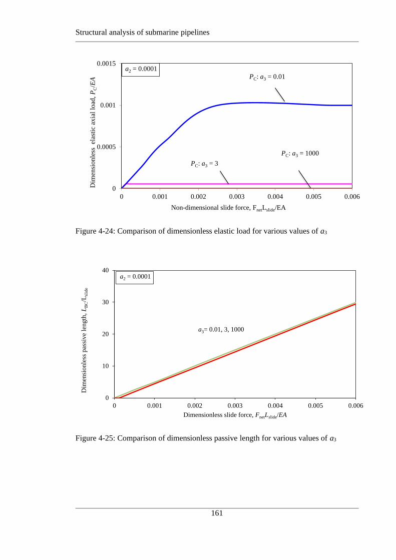
Structural analysis of submarine pipelines
161
0
0.0005
0.001
0.0015
0 0.001 0.002 0.003 0.004 0.005 0.006
Dim
ensi
on
less
el
asti
c ax
ial
load
, P
C/E
A
Non-dimensional slide force, FnetLslide/EA
a2 = 0.0001
PC: a3 = 0.01
PC: a3 = 3
PC: a3 = 1000
Figure 4-24: Comparison of dimensionless elastic load for various values of a3
0
10
20
30
40
0 0.001 0.002 0.003 0.004 0.005 0.006
Dim
ensi
on
less
pas
siv
e le
ngth
, L
BC/L
slid
e
Dimensionless slide force, FnetLslide/EA
a2 = 0.0001
a3= 0.01, 3, 1000
Figure 4-25: Comparison of dimensionless passive length for various values of a3

Structural analysis of submarine pipelines
162
0
0.02
0.04
0.06
0.08
0 0.001 0.002 0.003 0.004 0.005 0.006
Dim
ensi
on
less
pea
k d
isp
lace
men
t, u
A/L
slid
e
Dimensionless slide force, FnetLslide/EA
a2 = 0.0001
a3= 3, 1000
a3= 0.01
Figure 4-26: Comparison of dimensionless peak displacement for various values of a3
0
0.002
0.004
0.006
0.008
0.01
0.012
0 0.001 0.002 0.003 0.004 0.005 0.006
Dim
ensi
on
less
ela
stic
ax
ial
dis
pla
cem
ent,
uc/
Lsl
ide
Dimensionless slide force, FnetLslide/EA
a2 = 0.0001a3= 0.01
a3= 3, 1000
Figure 4-27: Comparison of dimensionless elastic displacement for various values of a3

Structural analysis of submarine pipelines
163
1.00E-08
1.00E-06
1.00E-04
1.00E-02
1.00E+00
1.00E+02
10.00 100.00 1000.00 10000.00 100000.00
Dim
ensi
onle
ss d
ispla
cem
ent,
u/L
slid
e
Dimensionless slide length, Lslide/D
u_A/L_slide
u_B/L_slide
u_C/L_slide
μ =0.3
Figure 4-28: Effect of normalised slide length on normalised displacements
1.00E-08
1.00E-06
1.00E-04
1.00E-02
1.00E+00
10.00 100.00 1000.00 10000.00 100000.00
Dim
ensi
onle
ss a
xial
loa
d, P
/EA
Dimensionless slide length, Lslide/D
P_B/EA
P_C/EA
μ =0.3
Figure 4-29: Effect of normalised slide length on normalised axial load

Structural analysis of submarine pipelines
164
0
0.001
0.002
0.003
0 200 400 600 800 1000
Ax
ial
com
pre
ssiv
e st
rain
, P
/EA
=ε
(%)
Along the length, x/D
Active slide
zone
Elastic zone
Passive slide
zone
a1 = 0.0000471a2 = 0.0000149a3 = 2.526
Figure 4-30: Dimensionless axial load profile for a slide of Lslide/D = 100
0
0.00001
0.00002
0.00003
0.00004
0 200 400 600
Dim
ensi
on
less
ax
ial
dis
pla
cem
ent,
u /
Lsl
ide
Along the length, x/D
Active slide zone
Passive
slide zone
Elastic zone
a1 = 0.0000471a2 = 0.0000149a3 = 2.526
Figure 4-31: Dimensionless displacement profile for a slide of Lslide/D = 100

Structural analysis of submarine pipelines
165
-0.00002
0
0.00002
0.00004
0.00006
0 200 400 600 800 1000
Dim
ensi
onle
ss a
xia
l fr
icti
onal
res
ista
nce
,
FL
slid
e/
EA
Along the length, x/D
Elastic zone
Passive slide
zone
Active slide zone
a1 = 0.0000471a2 = 0.0000149a3 = 2.526
Figure 4-32: Dimensionless frictional resistance profile for a slide of Lslide/D = 100
0
0.005
0.01
0.015
0 500 1000 1500 2000
Ax
ial
com
pre
ssiv
e st
rain
, P
/EA
=ε
(%)
Along the length, x/D
Case A3,
Lslide/D = 500
Case A2,
Lslide/D = 300
Case A1,
Lslide/D = 100
Figure 4-33: Comparison of axial load profiles for different slide lengths
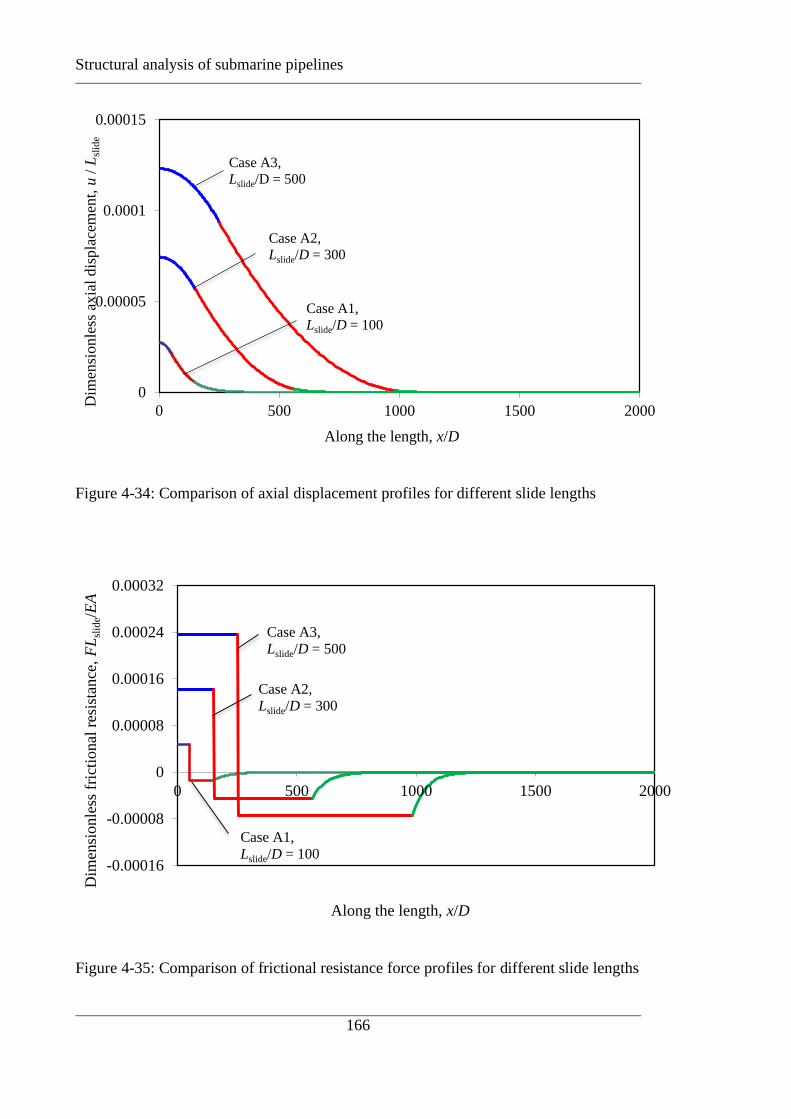
Structural analysis of submarine pipelines
166
0
0.00005
0.0001
0.00015
0 500 1000 1500 2000
Dim
ensi
on
less
ax
ial
dis
pla
cem
ent,
u/
Lsl
ide
Along the length, x/D
Case A3,
Lslide/D = 500
Case A2,
Lslide/D = 300
Case A1,
Lslide/D = 100
Figure 4-34: Comparison of axial displacement profiles for different slide lengths
-0.00016
-0.00008
0
0.00008
0.00016
0.00024
0.00032
0 500 1000 1500 2000
Dim
ensi
on
less
fri
ctio
nal
res
ista
nce
, F
Lsl
ide/
EA
Along the length, x/D
Case A3,
Lslide/D = 500
Case A2,
Lslide/D = 300
Case A1,
Lslide/D = 100
Figure 4-35: Comparison of frictional resistance force profiles for different slide lengths

Structural analysis of submarine pipelines
167
Axial slide loading
Passive plastic soil response Elastic soil response
B CLBC L∞Axial slide loading
Passive plastic soil response Elastic soil response
B CLBC L∞
Passive plastic soil response Elastic soil response
B CLBC L∞
1 m
Length considered for this study 5,000 m
Figure 4-36: Finite element model for pipeline soil interaction
0
0.00005
0.0001
0.00015
0 200 400 600 800 1000 1200 1400 1600
Dim
ensi
on
less
ax
ial
dis
pla
cem
ent,
u/
Lsl
ide
Along the length, x/D
Case A3
Case A2
Case A1
Analytical solution ( solid lines)
Numericall solution ( triangles)
Figure 4-37: Comparison of normalised axial displacements from analytical and FE
solutions
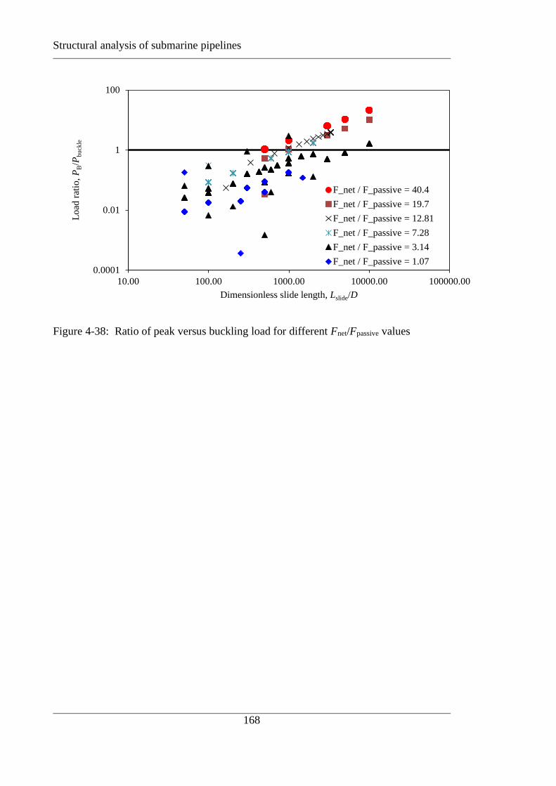
Structural analysis of submarine pipelines
168
0.0001
0.01
1
100
10.00 100.00 1000.00 10000.00 100000.00
Load
rat
io,
PB/P
bu
ckle
Dimensionless slide length, Lslide/D
F_net / F_passive = 40.4
F_net / F_passive = 19.7
F_net / F_passive = 12.81
F_net / F_passive = 7.28
F_net / F_passive = 3.14
F_net / F_passive = 1.07
Figure 4-38: Ratio of peak versus buckling load for different Fnet/Fpassive values

Structural analysis of submarine pipelines
169

Structural analysis of submarine pipelines
170
Structural analysis of submarine pipelines
171
PARAMETRIC SOLUTION OF LATERAL
BUCKLING OF SUBMARINE PIPELINES
5.1 INTRODUCTION
With the depletion of onshore and shallow offshore hydrocarbon reserves, the present oil
and gas industry is moving into the deeper sea. Deep sea developments generally include
a number of wells linked by flowlines, in addition to an export pipeline to onshore
production facilities. Deepwater pipelines are laid on the seabed and are usually left
unburied. In operation they are subjected to cycles of high temperature and high pressure.
This raises the possibility of on-bottom buckling or incremental axial displacement
(walking) of the pipelines (Carr et al. 2006)
Allan (1968) proposed a solution for the critical buckling load for vertical mode for a thin
strip with an imperfection at the centre under axial compressive load on a flat bed. Little
further work has been done to modify or include other parameters into the simple formula
given by Allan (1968).
Hobbs (1981, 1984) solution for a straight pipeline is still considered to be the design
guideline for buckling phenomena related to on-bottom pipelines. Both upheaval and
lateral critical buckling loads had been determined and expressed as a function of the
length of the buckle. For upheaval buckling it was assumed that the bending moment and
slope at the lift-off point is zero. For lateral buckling the lateral resistance is assumed
fully mobilised and the zero slope condition at the end of the buckle is replaced by a shear
force condition there. The buckling solutions proposed by Hobbs was based on the Kerr’s
Structural analysis of submarine pipelines
172
(1974, 1978) studies on the buckling of railway tracks, assuming a rigid foundation with
a constant frictional resistance.
Maltby & Calladine (1995) extended Hobbs’ solution for a straight pipe on a rigid seabed
by including an initial out of straightness of the pipe. They related the critical buckling
load to the central height (or imperfection) of the pipe above the seabed. They also
proposed a solution for lateral buckling of an imperfect pipe on a seabed with a non-linear
mobilisation of lateral resistance. More details of their work has been provided in the
following sections.
Croll (1997) derived the critical vertical buckling load of a straight pipe on flat seabed,
imperfect pipe on a point protrusion support and imperfect pipe on a continuous support.
Similarly, Tran & Taylor (1996) expressed the critical upheaval buckling load of an
imperfect pipe on a continuous support, on an isolated prop support and on a filled-prop
support as a function of Hobbs’s (1984) solution. Hetényi (1946) proposed a critical
buckling load solution for a bar under simultaneous axial and transverse loading. In that
model the bar was considered to be straight and lying on an elastic foundation under axial
compression.
Joint industry projects (JIPs) such as the previous HOTPIPE and subsequent SAFEBUCK
projects developed guidelines addressing the buckling phenomena related to HT/HP
pipelines ( Collberg et al. 2005, Bruton and Carr 2011). In these projects the buckling of
subsea pipelines subjected to internal pressure and temperature changes was investigated.
SAFEBUCK project outlined a design approach that addresses the inherent uncertainties
of the lateral buckling problem in a safe and quantifiable way (Bruton and Carr 2011). .
Submarine pipelines that are vulnerable to Euler buckling in the horizontal / lateral plane
are considered in this project. Hobbs (1981, 1984) solutions were adopted to provide
Structural analysis of submarine pipelines
173
analytical solution of lateral buckling and thereafter numerical solution was provided to
verify the analytical model.
A key step during the design of a HP/HT pipeline is to assess whether the pipeline will
be susceptible to on-bottom buckling. If buckling is likely, then the design must ensure
that buckles will form safely and reliably at a suitable spacing to absorb the expansion,
without overstressing the pipeline or leading to fatigue. A key element of this analysis is
assessment of the critical load at which buckling will occur. This load is then compared
with the expansion forces created by the constrained expansion created by changes in
pressure and temperature.
These solutions are simple and easy to use without any complexity of the soil-pipe
interaction. However, in practice the geotechnical parameters play a role, along with the
as laid geometry and pipe material, in the buckling behaviour of submarine pipelines.
This study evaluates the effects of as laid geometry of the pipe, ultimate lateral and axial
soil resistances and pipe-soil stiffness on the critical buckling load. At the end an attempt
is made to include all the relevant parameters into a single correlation, which then can be
used to predict the buckling load required.
Table 5-1 summarises the assumptions and expressions for the critical buckling load of
submarine pipelines given by various researchers over the last two decades. The aim of
this study is to provide insight into how the axial and lateral components of pipe-soil
stiffness and limiting resistance affect the lateral buckling response, and to derive new
expressions for the critical buckling load that take account of these components of pipe-
soil interaction.

Structural analysis of submarine pipelines
174
5.2 PROBLEM DEFINITION AND NOTATIONS
Buckling analysis of pipelines has created considerable interest in the past due to the
complexities involved in the analysis. JIP projects (e.g. Collberg et al. 2005, Burton &
Carr 2011) have provided a general overview of buckling phenomena and solutions
derived from classical theory. However, the separate effects of soil-pipeline interaction,
pipe material and geometry on the buckling initiation load were not properly identified
and discussed. This paper presents results of detailed numerical analyses carried out to
investigate the effects of geotechnical and non-geotechnical parameters on the critical
lateral buckling load of submarine pipelines. The analyses were carried out in two steps.
In the first step, the pipe response was investigated using elastic-plastic lateral springs
attached along a pipe with a lateral out-of-straightness (OOS) but without any initial
stress. The numerical solutions were found to match theory well, although it was found
that the classical theories do not allow for the effect of lateral soil stiffness. Hence, the
classical solutions were extended, based on the results of the analyses, to express the
critical buckling load non-dimensionally as a function of a soil stiffness factor. In the
second set of analyses, axial soil elements were introduced into the previous analyses but
the pipe was considered without any initial stress. This allowed another non-
dimensionalised expression of critical buckling load to be formulated, incorporating
factors representing the axial and lateral soil stiffnesses and ultimate resistances, in
addition to the initial OOS of the pipeline for a range of pipe parameters. The third set of
analyses were the extension of the second set but with the initial stress in the pipe.
The pipe was defined by diameter, D, thickness, t, Young’s modulus, E, Yield stress, σy,
with a OOS, Δ, nominal length of the OOS, L, and the bending rigidity, EI and axial
stiffness, EA can be calculated. The loads per unit length on the pipeline are defined as
horizontal limiting load per unit length H, parallel to the y-axis and axial limiting load
Structural analysis of submarine pipelines
175
per unit length F parallel to the x-axis (see Figure 5-1). Likewise the elastic slips in the x
and y axes are δx and δy, respectively as shown in the same Figure 5-1 and the
displacements in the x and y axes are δX and δY respectively. The stiffnesses in the two
directions ky, kx are defined as the limiting load (per unit length) per unit displacement,
so with typical units of kN/m2 or kPa, and are expressed as ky = H/ δy for horizontal/lateral
direction and kx = F/ δx for axial direction. The output of the analyses was the critical
buckling load and expressed as Pcr. The dimensional analysis of buckling is discussed in
the following section.
5.3 DIMENSIONAL ANALYSIS
The aim of this study is to provide generic design charts expressing the resulting critical
buckling load of the pipeline as a function of the various input parameters. Therefore,
dimensional analysis is a particularly suitable starting point for this study. Although this
kind of analysis alone does not usually lead to a complete solution of the problem, it
increases the understanding by laying the foundation of design of numerical and
experimental simulations (Massey 1971).
A summary of the various input parameters considered for the analyses is provided in
Table 5-2, along with the main output parameter, which is the critical buckling load , Pcr.
There are eight input variables, but only two dimensional outputs: buckling load (kN) and
nominal length of the OOS (m). As such, the output may be expressed, non-
dimensionalised, as a function of six independent dimensionless groups. Many different
combinations of the input variables are available, but the underlying dimensions of this
problems are length and force. Therefore, here it has been decided to use the bending
rigidity EI, as standard force and a length that approximates the pipeline diameter D. For

Structural analysis of submarine pipelines
176
pipes of moderate wall thicknesses, the nominal diameter of the pipe may be
approximated as
𝐷 ≈ √8𝐸𝐼
𝐸𝐴
(5-1)
For the normalisations used in the paper D refers to the external diameter and the true
(exact) values of EI and EA have been used.
The other length quantities are the out of straightness parameter , and the nominal length
L of the out of straight section of the pipeline. A more precise definition of L is provided
later, with respect to the actual pipeline profile adopted in the numerical analyses. These
length quantities may be normalised by the approximate pipeline diameter, although it is
rather more convenient from an application perspective to consider /L (equivalent to
/D divided by L/D), rather than /D.
The critical buckling load may then be expressed as
𝑃𝑐𝑟𝛥2
𝐸𝐼= 𝑔 (
𝛥
𝐿,
𝐻𝛥3
𝐸𝐼,
𝛥
√8𝐸𝐼/𝐸𝐴,
𝑘𝑦
𝐻√
8𝐸𝐼
𝐸𝐴,
𝐹
𝐻,
𝑘𝑥
𝐹√
8𝐸𝐼
𝐸𝐴)
(5-2)
This expression is a generalisation of the buckling solution provided by Maltby &
Calladine (1995) for upheaval buckling of a pipe of weight (per unit length) W resting
on a rigid seabed. Here, where lateral buckling is being considered, the lateral resistance
H replaces the pipeline weight. In addition, the pipe cross-sectional rigidity EA, axial
resistance F and corresponding axial and lateral pipe-soil stiffnesses are considered. Also,
elastic slips in the lateral and axial directions were considered by dividing elastic
stiffnesses by the corresponding forces. These length quantities may be normalised by the
approximate pipeline diameter.

Structural analysis of submarine pipelines
177
Before starting the numerical analyses it is useful to discuss the theory proposed by
Maltby & Calladine (1995). They described an experimental study of some aspects of
upheaval buckling of buried pipelines by small-scale model. Various theories of upheaval
buckling with rigid base were reviewed in their study and the experimental observations
on the growth of initial imperfection in the pipe under constant increasing axial load, and
the formation of unstable buckles were in good agreement with the findings of Tvergaad
and Needleman (1980) on railway track.
For this analyses it is helpful to consider the Maltby & Calladine (1995) buckling solution,
as summarised in Table 5-1, replacing the pipe weight by the limiting lateral resistance
of the soil. They gave the critical load for a straight pipe resting on a rigid (smooth) seabed
as
=
EIHPcr
96.3
(5-3)
with the corresponding buckle length expressed as
𝐿 = 4.51 (𝛥𝐸𝐼
𝐻)
1/4
(5-4)
Rearranging equation (5-3) gives
𝑃𝑐𝑟𝛥2
𝐸𝐼= 3.96√
𝐻𝛥3
𝐸𝐼
(5-5)
And rearranging equation (5-4) gives

Structural analysis of submarine pipelines
178
𝛥
𝐿=
1
4.51(
𝐻𝛥3
𝐸𝐼)
1/4
or 4.51𝛥
𝐿(
𝐻𝛥3
𝐸𝐼)
−1/4
= 1 (5-6)
The boundary conditions in the Malty & Calladine (1995) solution led to a constraint on
the magnitude of the buckle length L in terms of H and EI. However, in the more general
analysis presented here, the initial length L of the out of straight section of pipeline is an
independent input variable, although also reflects closely the length of the buckle that
transpires.
An expression for the critical buckling load that reflects both H and L may be obtained
by dividing the right hand side of equation (5-5) by some power, n, of equation (5-6), to
give
𝑃𝑐𝑟𝛥2
𝐸𝐼= 3.96 (
𝐻𝛥3
𝐸𝐼)
1/2
(𝐻𝛥3
𝐸𝐼)
𝑛/4
. (4.51𝛥
𝐿)
−𝑛
(5-7)
The relative contributions of H3/EI and /L may be ‘balanced’ by taking n = 2/3, which
results in a final expression for the critical buckling load of
𝑃𝑐𝑟𝛥2
𝐸𝐼= 1.45 (
𝛥
𝐿)
−2/3
(𝐻 ⋅ 𝛥3
𝐸𝐼)
2/3
(5-8)
Justification for such balancing of the contributions from H3/EI and /L is provided later
in light of the numerical analysis results.
5.4 METHODOLOGY
To investigate the buckling behaviour of submarine pipelines, and an appropriate form
for the generalised relationship of equation (5-2), finite element analysis was performed
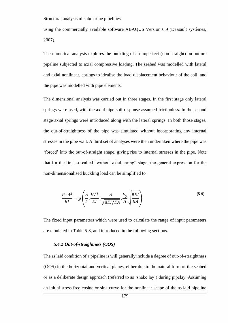
Structural analysis of submarine pipelines
179
using the commercially available software ABAQUS Version 6.9 (Dassault systèmes,
2007).
The numerical analysis explores the buckling of an imperfect (non-straight) on-bottom
pipeline subjected to axial compressive loading. The seabed was modelled with lateral
and axial nonlinear, springs to idealise the load-displacement behaviour of the soil, and
the pipe was modelled with pipe elements.
The dimensional analysis was carried out in three stages. In the first stage only lateral
springs were used, with the axial pipe-soil response assumed frictionless. In the second
stage axial springs were introduced along with the lateral springs. In both those stages,
the out-of-straightness of the pipe was simulated without incorporating any internal
stresses in the pipe wall. A third set of analyses were then undertaken where the pipe was
‘forced’ into the out-of-straight shape, giving rise to internal stresses in the pipe. Note
that for the first, so-called “without-axial-spring” stage, the general expression for the
non-dimensionalised buckling load can be simplified to
𝑃𝑐𝑟𝛥2
𝐸𝐼= 𝑔 (
𝛥
𝐿,𝐻𝛥3
𝐸𝐼,
𝛥
√8𝐸𝐼/𝐸𝐴,𝑘𝑦
𝐻√
8𝐸𝐼
𝐸𝐴)
(5-9)
The fixed input parameters which were used to calculate the range of input parameters
are tabulated in Table 5-3, and introduced in the following sections.
5.4.2 Out-of-straightness (OOS)
The as laid condition of a pipeline is will generally include a degree of out-of-straightness
(OOS) in the horizontal and vertical planes, either due to the natural form of the seabed
or as a deliberate design approach (referred to as ‘snake lay’) during pipelay. Assuming
an initial stress free cosine or sine curve for the nonlinear shape of the as laid pipeline
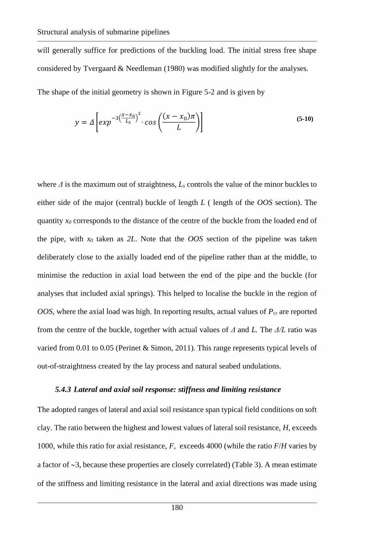
Structural analysis of submarine pipelines
180
will generally suffice for predictions of the buckling load. The initial stress free shape
considered by Tvergaard & Needleman (1980) was modified slightly for the analyses.
The shape of the initial geometry is shown in Figure 5-2 and is given by
𝑦 = 𝛥 [𝑒𝑥𝑝−3(
𝑥−𝑥0𝐿𝑠
)2
⋅ 𝑐𝑜𝑠 ((𝑥 − 𝑥0)𝜋
𝐿)] (5-10)
where Δ is the maximum out of straightness, Ls controls the value of the minor buckles to
either side of the major (central) buckle of length L ( length of the OOS section). The
quantity x0 corresponds to the distance of the centre of the buckle from the loaded end of
the pipe, with x0 taken as 2L. Note that the OOS section of the pipeline was taken
deliberately close to the axially loaded end of the pipeline rather than at the middle, to
minimise the reduction in axial load between the end of the pipe and the buckle (for
analyses that included axial springs). This helped to localise the buckle in the region of
OOS, where the axial load was high. In reporting results, actual values of Pcr are reported
from the centre of the buckle, together with actual values of Δ and L. The Δ/L ratio was
varied from 0.01 to 0.05 (Perinet & Simon, 2011). This range represents typical levels of
out-of-straightness created by the lay process and natural seabed undulations.
5.4.3 Lateral and axial soil response: stiffness and limiting resistance
The adopted ranges of lateral and axial soil resistance span typical field conditions on soft
clay. The ratio between the highest and lowest values of lateral soil resistance, H, exceeds
1000, while this ratio for axial resistance, F, exceeds 4000 (while the ratio F/H varies by
a factor of 3, because these properties are closely correlated) (Table 3). A mean estimate
of the stiffness and limiting resistance in the lateral and axial directions was made using

Structural analysis of submarine pipelines
181
the parameters given in Table 5-4, and calculation methods based on elastic and plasticity
(Guha et al., 2016, Randolph & White, 2008, Merified et al., 2008) . These typical values
were then extended to create the wider range spanned by the parametric study.
The axial pipe-soil stiffness is given as (Guha et al., 2016)
𝑘𝑥 = 𝑚𝐷𝑠𝑖𝑛𝜃𝐷 (5-11)
where kx is the axial soil stiffness, m is the constant of shear modulus (G = mz, z is the
depth below the pipe), and θD is the embedment angle of the pipe as discussed in the
previous chapter. The axial elastic stiffness, kx span a range of 0.04 to > 200 kN/m2 was
considered here.
The limiting value of the axial force is
𝐹 = 𝛼𝑠𝑢_𝑠𝑒𝑎𝑏𝑒𝑑𝐷𝜃𝐷 (5-12)
where F is the ultimate axial frictional resistance of the soil per unit length, α is adhesion
factor, undrained shear stress varies with depth z as su_seabed = kz, D is the diameter of the
pipe, θD is the subtended contact angle (White & Randolph, 2007).
The lateral pipe-soil stiffness, ky was estimated by dividing the ultimate lateral resistance,
H, by elastic slip, δy . For this study δy in the range of 0.05D to 0.5D was considered. As
highlighted in the paper Guha et al. (2016) that lateral and vertical stiffnesses predicted
numerically are rather higher. The higher values for homogeneous soil modulus may be
attributed, at least partly, to the limited layer modelled numerically. Therefore, a range of
0-20% was proposed in the paper (Guha et al., 2016) for vertical and lateral elastic
stiffnesses. Therefore, a slightly higher value of kx/ky =0.7 was adopted in the present
chapter.
Structural analysis of submarine pipelines
182
5.4.4 Numerical method
To analyse the problem of buckling associated with material nonlinearity and geometric
nonlinearity prior to buckling an advanced method such as the Riks algorithm (Riks,
1979) is very useful. The Riks method is a static stress-based analysis method which uses
the load magnitude as an additional unknown; it solves the load and deflection
simultaneously. Geometrically nonlinear static problems sometimes involve buckling or
collapse behaviour, where the load-deflection response shows a negative stiffness and the
structure must release strain energy to remain in equilibrium. The Riks algorithm allows
for the complete load-deflection curve to be determined including a reversal of load path.
Therefore with this method it is possible to study an instability phenomenon such as
bifurcation and snap-through buckling and obtain a complete solution of the post-
buckling response. This method is used for cases where the loading is proportional, that
is, where a single scalar parameter governs the load magnitude. This is very important for
the analysis of structures carrying de-stabilising loads such as axial load in a pipeline,
column or pile. The advantage of the method is that the solution is viewed as the discovery
of a single equilibrium path by the loading parameters and the nodal variables. The
elegant solution comes by tracing the equilibrium path, as far as required.
To reduce the complexity of the problem and make a simple solution for the same, a
loading pattern is initially defined by a load vector (Pn), this load vector represents the
relative magnitude applied to the structure. Then a proportional load factor (λ) is applied
to all of these loads. The load proportionality factor is found out as the part of the solution.
The equilibrium equations may be expressed in terms of a vector representing the
displacement (u) and load factor. The total load can be expressed by the multiplication of
the load factor with the set of unit loads over the structure at any increment (n)

Structural analysis of submarine pipelines
183
n
total PP =
(5-13)
If there are internal loads available, then the expression becomes
n
total PPP −= int
(5-14)
The response of a structural system in discrete set of nonlinear equation can be expressed
as in the following form
0),( =uf
(5-15)
The nonlinear equilibrium path is represented in λ-u plane
𝑓(𝜆, 𝑢) = 𝑓(𝜁) (5-16)
These equations are solved in a series of steps or increments, starting from λ = 0 condition.
The nth step starts from a known solution on the equilibrium path in the solution space ζ
= (λ, u)T (Ragon et al., 2002) .This consists of two phases, Prediction phase and
Correction phase. In the prediction phase estimation is generated on the equilibrium path
𝜁0 = (𝜆𝑛+10 , 𝑢𝑛+1
0 )𝑇
(5-17)
With this starting point Newton-Raphson method is employed to find the next point on
the equilibrium path. The size of each step is fixed with an arc length Δl. The general set
of equations for i-th iteration executed by each algorithm at step (n+1) is expressed as

Structural analysis of submarine pipelines
184
( ) ( )1
1
1
1
−
+
−
+ = i
n
i
n fDf (5-18)
( ) 01
1 =−
+
i
nc (5-19)
where
1
11
−
++ −= i
n
i
n , i = 1, 2, … (5-20)
and
=
−
+
−
+−
+u
ffDf
i
n
i
ni
n
)()()(
1
1
1
11
1
(5-21)
Equation (5-21) is the m x (m+1) Jacobian matrix of the system f(λ, u) = 0 and defines the
tangent stiffness of the structure in λ-u space. As mentioned above, an arc length Δl is
introduced in ABAQUS (Crisfield, 1981) which limits the length of the displacement
vector. This prevents the internal stress residual to become too large and iterating back
the solution onto the equilibrium path. In this modified algorithm a hypersphere is defined
with a locus on the λ-u plane as used by Knappett & Madabhushi (2009) for the lateral
response of piles to axial loading. The constrain equation is modified to
(𝜁𝑛+1𝑖 − 𝜁𝑛
∗)𝑇(𝜁𝑛+1𝑖 − 𝜁𝑛
∗) = 𝛥𝑙2
(5-22)
As mentioned earlier the (n+1)th increment will follow a two-stage procedure namely
prediction and correction stages. Starting from a known solution point from the nth
increment, ζ*n+1, the bounding radius or the arc-length Δl is defining the hypersphere and

Structural analysis of submarine pipelines
185
a prediction step is made to estimate ζ0n+1, on the bounding radius. At this stage
equilibrium conditions are checked for the newly defined point as the internal stresses
were generated by the external deflection. If the equilibrium condition is not satisfied,
Newton-Raphson iteration is used in the correction step for the point ζ0n+1 to the next
point ζ1n+1 and onwards as shown in Figure 5-3. This procedure continues until the
internal stresses are in equilibrium within certain tolerance.
For nonlinear buckling analysis modified Riks method is very popular. Torselleti et al.
(1999), as part of the Hotpipe project, carried out FE analysis of submarine pipeline
resting on flat seabed with ABAQUS. They employed RIKS method to compare the
analytical solution with their numerical results for initial imperfection and pipe material
properties. Sriskandarajah et al. (1999) employed arc-length method to investigate the
lateral buckling influenced by the lay induced imperfection. In risk based design and
reliability analysis of submarine pipelines subjected to global buckling, FE analyses with
ABAQUS was also very popular (Maschner & Wang, 2008, Peek & Yun, 2007) with
beam or pipe elements and were mainly used for structural analysis of long pipelines for
numerical advantages (Torselleti et al.,1999; Peek & Yun ,2007; Maschner & Wang,
2008, Odina, & Tan, 2009, Chee et al., 2019, Chee et al., 2018). The details of beam and
pipe elements and the pipe-soil interaction are discussed in the following sections.
Comparisons of static, dynamic and Riks methods were presented by Sriskandarajah et
al. (1999), Zhou et al., (2019) and Wang et al. (2015), revealing that the three methods
are in good agreement to predict the peak buckling load.
5.4.5 Beam element as pipe model
According to ABAQUS manuals, a beam is defined by an element in which assumptions
are made so that the problem is reduced to one dimension mathematically: the primary

Structural analysis of submarine pipelines
186
solution variables are functions of position along the beam axis and the shortest distance
from the axis to any point in the continuum is smaller than typical lengths along the axis
of the element. The element library in ABAQUS contains several types of beam elements
and these are generally divided by the approach to beam theory into three parts: Euler-
Bernoulli beam, Timoshenko beam, and hybrid beam elements as shown in the Figure
5-4. Firstly, the Euler-Bernoulli beam theory is a classic and simplest in that it is based
on the assumption that cross-section does not deform in its plane or warp out of its plane
and this cross-sectional plane remains normal to the beam axis. Since this beam element
can be used to simulate beams for large axial strains as well as large rotations, this beam
theory supplies generally satisfactory results for slender beams. The ABAQUS beam
element library provides B23, B33, and so forth, as this type of beam.
The Timoshenko beam theory allows transverse shear strain that is the cross-section may
not necessarily remain normal to the beam axis. This approach can be useful for thicker
beams whose shear flexibility may be important. Also, this is effective to simulate thin
beams where Euler- Bernoulli theory is accurate. There are several element types in the
ABAQUS beam element library, such as B21, B22, B31, B32, etc. The hybrid beam
elements in ABAQUS are designed to handle very slender situations where the axial
stiffness of the beam is very large compared to the bending stiffness.
The pipe elements in ABAQUS such as PIPE21, PIPE22, PIPE31, PIPE32, etc and their
hybrids are available with hollow, thin-walled, circular section. The hoop stress caused
by internal or external pressure loading in the pipe is included. The main purpose of these
is to provide for the subsequent difference in yield when a point in the section is subjected
to axial tension or compression stress due to its nonzero hoop stress component causing
an asymmetry in the section’s response to inelastic bending as shown in the Figure 5-5.

Structural analysis of submarine pipelines
187
The hybrid pipe elements such as, PIPE31H, PIPE32H, etc are used where it is difficult
to compute the axial and transverse shear forces in the beam by the FE displacement
method. This kind of problems of arises in geometrically nonlinear analysis when the
element undergoes large rotations and is very rigid in axial and transverse shear
deformation, such as flexible long pipe or cables. The hybrid elements use a more
generalised formulation in which the axial and transverse shear forces in the elements are
included, along with the nodal displacements and rotations, as primary variables.
Therefore, PIPE31H was selected as the appropriate element for this kind of geometric
nonlinear analysis due to the option of applicability of internal and external pressure for
these elements for future research where study can be under taken to investigate the effect
of internal and external pressure on the buckling response ( Zhou et al., 2019, Peek &
Yun, 2007, Odina & Tan, 2009).
5.4.6 Pipe-soil interaction model
Traditionally, the buckling of submarine pipelines and the seismic fault crossing effect
on buried pipelines idealises soil behaviour using discrete springs to model the pipe-soil
interaction based on the concept of subgrade reactions proposed by Winkler (Odina &
Tan, 2009). In that model the soil is represented as series of independent springs attached
to the nodes of the pipeline. An elasto-plastic spring is generally used to idealise the force-
displacement response at the pipe surface. The spring relationships in all the three
direction are defined by the maximum force per unit length at the soil pipe interface and
the ultimate mobilization displacement. The force-displacement model considered, for all
the three directions is defined in the section below. For nonlinear structural analysis pipe
soil interaction (PSI) and spring elements are widely used.

Structural analysis of submarine pipelines
188
The axial, lateral and vertical soil pipe interaction was modeled with nonlinear springs
(SPRING1) available in ABAQUS, which link each node to a fixed reference point (the
ground). The nonlinearity of the springs was defined separately in the input code. The
relative displacement across a SPRING element is the ith component of displacement of
the spring’s node and can be given by:
𝛥𝑢 = 𝑢𝑖
(5-23)
where i is defined in the spring input code and is in the local direction of the model. In
ABAQUS lateral and axial springs are directly oriented towards the global coordinates.
In this scenario if the pipe element is deformed in the global x-axis, the axial soil stiffness
will contribute to both axial and lateral stiffness component. At the same time lateral soil
stiffness may affect the axial component and lateral component. Therefore, special
computing may be employed to eliminate this issue (Sollund & Vedeld, K., 2014).
However, to predict the peak buckling load in the pipe this issue has minimum impact.
Therefore, for the simplicity purposes this has been ignored here.
5.4.7 Model discretization and boundary conditions
To carry out FE analysis the pipe was idealised as an elastic-plastic beam resting on a
nonlinear foundation with one end on the roller and the other end was pinned. At the roller
end a displacement was given which idealises the compressive load in the axial direction.
A lateral imperfection was deliberately introduced into the pipe to investigate the effect
of OOS on the critical buckling load. The whole length of 1 kilometre of the pipeline was
divided into small elements of approximately 1 metre length and at each node of the
element bilinear springs were attached, which represents the soil restraints in the lateral
and axial directions. The effect of element size was also investigated by changing the

Structural analysis of submarine pipelines
189
element size and thereby changing the number of springs. However, the above
discretisation was used finally as an appropriate compromise between accuracy and
economy.
5.5 CASE STUDY
Based on the model described in the above sections a simple case study was performed
to check the sensitivity of the model in a series of buckling analyses. In the first case the
axial springs were not attached and the OOS was considered to be initially stress free.
Only lateral springs were attached to analyse the behaviour of lateral buckling during an
axial compressive loading. The effects of temperature, pressure and external loads were
incorporated by displacing the end of the modelled section of pipe axially in compression.
5.5.2 Example analyses – effect of OOS
With the model discussed in the above section an example analysis was carried out to
check the effect of input parameters on the expected outcomes. For this example a pipe
with D = 0.152 m (6″) was considered with D/t ratio as 30.3 and σy / E as 0.002. The pipe
has a bending rigidity, EI of 1.24 MNm2. A bi-linear soil model was considered with
normalised limiting lateral resistance, HΔ3/EI = 4.24x10-05 and elastic stiffness, ky/H√
(8EI/EA) = 16.66 (H = 424 N/m and δy = 0.008 m). The ratio of Δ/L was varied from 0.01
to 0.05.
Axial load-displacement curves for various Δ/L ratios are compared in Figure 5-6, with
the displacement of the loading end plotted against the load at the central node of the
buckle.For smaller OOS the peak buckling load is higher and the instability is more
prominent. With increasing OOS the axial load-displacement response does not show
‘snap-through’. The summary of peak loads is plotted as shown in Figure 5-7. It depicts
the variation of peak buckling load with OOS. The peak load at Δ/L = 0.01 is 3.5 time
Structural analysis of submarine pipelines
190
higher than the peak load at Δ/L = 0.05. With increasing Δ/L ratio the load required for
buckling decreases. Therefore, it agrees with the previous findings that OOS tends to
reduce the critical buckling load as presented by others (Maltby & Calladine, 1995, Croll,
1997, Taylor & Tran 1996, Zhou et al. 2019).
The relationships between axial load and lateral offset of the midpoint of the buckle are
plotted for various Δ/L ratios in Figure 5-8. The lateral displacement of the midpoint of
the buckle is plotted including the initial OOS values in order to show the effect of the
total lateral offset on the sustainable buckling load. Just as for the axial load-displacement
case higher OOS does not allow ‘snap-through’ buckling. After the peak load reaches its
maximum value it reduces and merges with the peak load with higher Δ/L ratios.
Figure 5-9 shows the lateral friction distribution at the buckling initiation along the length
of the pipeline for Δ/L = 0.01 to 0.05. The ultimate lateral resistance was fully mobilised
through the central lobe prior to the onset of buckling for /L > 0.01, and for /L = 0.05
the ultimate resistance was also fully mobilised in the secondary lobes when buckling
occurred. These results show the significance of initial soil condition and effect of OOS
on the buckle response.
The comparison between the initial shape and the corresponding displaced shapes of the
buckles at the peak load are shown in Figure 5-10. A smaller OOS requires a larger load
to mobilise the elastic limit. Figure 5-9 show that a larger OOS is more prone to buckle
and the corresponding lateral displacement is higher for smaller OOS. It is evident from
Figure 5-11 that the lateral offset of the pipe is very low (0.0093 m) for Δ/L = 0.01 when
buckling occurs, and has only just exceeded the elastic limit within the lateral force-
displacement response. However, the lateral displacement at which buckling occurs
increases with increasing OOS. For Δ/L = 0.05 the offset of the midpoint of the buckle at
peak load is 47 times higher than that for Δ/L = 0.01.

Structural analysis of submarine pipelines
191
5.5.3 Example analyses – effect of soil resistance
To show the effect of lateral limiting friction on the peak load, FE results for three
different limiting lateral resistances (H = 100, 200 and 424 N/m) were compared. Figure
5-12 illustrates the influence of the lateral limiting resistance on the peak load of the
middle node. It is evident that the buckling initiation is significantly influenced by the
lateral limiting residence. As the limiting lateral resistance reduces from 424 N/m to 100
N/m (⁓ 4 fold decrease) the peak load reduces by a factor slightly higher than 2.
Correspondingly for a lower OOS the limiting lateral soil resistance has greater impact
on peak buckling than for a higher OOS. This is because the higher OOS does not lead to
‘snap-through’ buckling.
The analytical solution proposed by Maltby & Calladine (1995) for H = 424 N/m was
plotted on the same graph (dotted line) to compare with the FE solutions. On the same
graph (Figure 5-12) the dimensionless modified Maltby & Calladine (1995) results for H
= 424 N/m was also plotted. It is evident that the FE results are lower than the analytical
results because of the initial assumptions in the analytical modelling: (1) analytical
solution considered a fully mobilised lateral limiting friction; and (2) In the FE solution
the initial shape similar to mode 3 (of Hobbs solution) was considered predicted by
equation (5-3) whereas for the analytical solution mode 1 (of Hobbs solution) was
considered by Maltby & Calladine (1995).
To show the effect of lateral soil stiffness (or reverse of elastic slip) on the peak load a
series of analyses were carried out for elastic stiffness parameter of the lateral spring, ky
ranging between 0.5 – 5 kN/m2. This was achieved by varying the elastic slip, δy between
0.05D – 0.5D for H = 424 N/m and EI = 1.24 MNm2. Figure 5-13 illustrates the effect of
elastic slip on the peak load. The elastic slip was normalised by the diameter of the pipe
Structural analysis of submarine pipelines
192
(0.152 m or 6”). With increasing elastic slip (decreasing elastic stiffness) of the soil the
peak load reduces (Zhou et al. 2019).
Before starting the parametric study to explore the cases of ‘without axial resistance’,
‘with axial resistance and without initial stress’ and ‘with axial resistance and with initial
stress’, a simple graph was plotted to show the effect of these three cases on the
normalised peak buckling load . For this analysis similar input parameters were chosen
as above, just changing the axial soil resistance, but keeping F/H at 0.3. Also for the ‘with
axial and with initial stress’ the pipe was pre-stressed before commencing the real
buckling simulation. Figure 5-14 shows the comparison of peak buckling load varying
with OOS for three different cases. Difference between the peak loads decrease
significantly with higher OOS. It is evident from the figure that peak load in the pipe is
higher with axial resistance and highest with axial resistance and initial stress. For an out-
of-straightness, = 2.5 m (/L = 0.05) the value of peak load for ‘with axial and without
initial stress’ is 1.43 times higher than that for ‘without axial’ case due to the addition of
axial springs (resistance) along the length of the pipeline. Similarly, initial stress in the
pipe increases the peak load further 1.11 times for the same value. Based on these
results a comprehensive parametric study was carried out in the next section.
5.6 RESULTS OF PARAMETRIC STUDY
Many numerical analyses were carried out for a range of cases to establish a general
relationship for the critical buckling load, Pcr. This load was found by analysis of the
responses from >200 separate analyses using a range of pipe and pipe-soil parameters,
including different Δ/L ratios. Pipe with three different diameter sizes of 0.152 m (6″),
0.304 m (12″) and 0.912 m (36″) with D/t ratio of 30, were considered. The results were
plotted in nondimensionalised manner all cases. First a design chart was proposed based
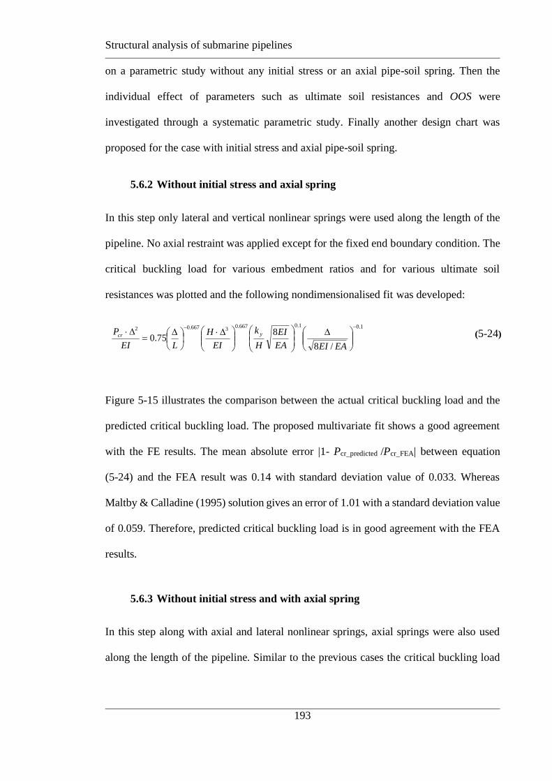
Structural analysis of submarine pipelines
193
on a parametric study without any initial stress or an axial pipe-soil spring. Then the
individual effect of parameters such as ultimate soil resistances and OOS were
investigated through a systematic parametric study. Finally another design chart was
proposed for the case with initial stress and axial pipe-soil spring.
5.6.2 Without initial stress and axial spring
In this step only lateral and vertical nonlinear springs were used along the length of the
pipeline. No axial restraint was applied except for the fixed end boundary condition. The
critical buckling load for various embedment ratios and for various ultimate soil
resistances was plotted and the following nondimensionalised fit was developed:
1.01.0667.03667.02
/8
875.0
−−
=
EAEIEA
EI
H
k
EI
H
LEI
P ycr (5-24)
Figure 5-15 illustrates the comparison between the actual critical buckling load and the
predicted critical buckling load. The proposed multivariate fit shows a good agreement
with the FE results. The mean absolute error |1- Pcr_predicted /Pcr_FEA| between equation
(5-24) and the FEA result was 0.14 with standard deviation value of 0.033. Whereas
Maltby & Calladine (1995) solution gives an error of 1.01 with a standard deviation value
of 0.059. Therefore, predicted critical buckling load is in good agreement with the FEA
results.
5.6.3 Without initial stress and with axial spring
In this step along with axial and lateral nonlinear springs, axial springs were also used
along the length of the pipeline. Similar to the previous cases the critical buckling load

Structural analysis of submarine pipelines
194
for different as-laid geometry of the pipes and for various ultimate soil resistances was
developed into a nondimensionalised fit:
𝑃𝑐𝑟 ∙ Δ2
𝐸𝐼= 1.15 (
Δ
𝐿)
−0.66
(H ∙ Δ3
𝐸𝐼)
0.66
(k𝑦
𝐻√
8𝐸𝐼
𝐸𝐴)
0.1
(Δ
√8𝐸𝐼/𝐸𝐴)
−0.1
(𝐹
𝐻)
−.017
(k𝑥
𝐹√
8𝐸𝐼
𝐸𝐴)
−0.12
(5-25)
This solution verifies the classical buckling solution and extends it with axial and lateral
soil stiffness terms. Figure 5-16 illustrates the comparison between the calculated and
predicted critical buckling load. The proposed multivariate fit shows good agreement with
the FE results. The mean absolute error |1- Pcr_predicted /Pcr_FEA| between equation (5-25)
and FEA result was found out to be 0.63 with a standard deviation value of 0.058, which
is again an improvement on Maltby & Calladine (1995), for which the mean error was
2.67 and value of standard deviation was 0.087.
However, the solution does not include the initial stress in the pipe due to its shape and
the axial component of the soil resistance. The following section adds these aspects.
5.6.4 With initial stress and axial springs
In the field due to the pipe lay process and any uneven seabed topography, the pipe gains
an OOS and hence the pipe is pre-stressed, prior to the addition of axial stresses. Initially
a straight pipe was chosen and then it was bent into the desired shape using equation (5-
10). This is called ‘pulled in place’ case. Thereafter, the soil springs were activated i.e.
the pipe was put in contact with the soil. It was anticipated that the pipe would rebound
slightly due to the elastic slip, as well as the redistribution of elastic stresses within the
pipe. Therefore, the buckle portion, particularly the central lobe and the mid-point of the
central lobe, was pushed slightly further – so that even after rebounding the shape it would
still provide the same OOS. The net effect was that the pipe was pre-stressed before

Structural analysis of submarine pipelines
195
commencing the real buckling. At this stage the springs along the length of the pipe were
deactivated and did not impose any resistance to the lateral displacement to achieve the
deformed shape. Thereafter, all the springs were activated and buckling analyses was
carried out, via displacement control simulation. Similar to the previous cases, the ratio
Δ/L was varied between 0.01 to 0.05 to cover a wide range of OOSs.
Finally, the effect of all soil parameters and the as-laid geometry on the critical lateral
buckling load of a pre-stressed pipeline is given by the nondimensionalised form as
𝑃𝑐𝑟.Δ2
𝐸𝐼= 1.35 (
Δ
𝐿)
−0.66
(H. Δ3
𝐸𝐼)
0.66
(k𝑦
𝐻√
8𝐸𝐼
𝐸𝐴)
0.1
(Δ
√8𝐸𝐼/𝐸𝐴)
−0.1
(F
𝐻)
−0.26
(k𝑥
𝐹√
8𝐸𝐼
𝐸𝐴)
−0.18
(5-26)
Figure 5-17 shows the comparison between the actual and the predicted normalised
critical buckling load of pre-stressed pipeline with similar seabed conditions and
geometry as above. The mean absolute error |1- Pcr_predicted /Pcr_FEA| between
equation
(5-26) and FEA result was 0.14 with a standard deviation value of 0.068, which is an
improvement on the Maltby & Calladine (1995) solution, for which the mean error was
0.58 and with a standard deviation value of 0.084. The multivariate fit shows good
agreement with the actual FE results. Lateral friction exists to restrain the pipe from
rebounding back for the pulled in place case, while there is no stress in the wished in
place case. During buckling the initial friction is first mobilized similar to the pulled in
place case. Then a higher axial force is needed to activate buckling. As for the wished in
place case, the axial compression directly causes the lateral friction to accumulate. As a
result, the buckling of the pulled in place case is delayed and more energy accumulates,
potentially leading to snap-through buckling (Zhou et al 2019). The increase in peak load

Structural analysis of submarine pipelines
196
due to initial stress in the pipe was also observed by the others (Zhou et al., 2019, Miles,
1998). Therefore, the results can be used by the designers to predict the buckling load of
an imperfect pipe laid on a soft seabed.
5.7 CONCLUSIONS
The chapter reports an investigation of the lateral buckling problem of on-bottom
pipeline subjected to axial compressive loading. A detailed prediction method based on a
multi-variate fit to the relevant dimensionless groups was developed to predict critical
buckling load. The seabed was idealised with horizontal, axial nonlinear springs to
idealise the load-displacement behaviour of the soil and the pipe was modelled with pipe
elements. Buckling was performed by a displacement controlled finite element method
with the modified Riks algorithm that is available in the commercial software ABAQUS.
In the first step the classical theories were verified with the numerical tool and a simple
multivariate fit was proposed by carrying out parametric study. Then in the next steps
actual analysis was carried out by incorporating the axial springs and the initial stress into
the numerical model. The results have been synthesised in a generic non-dimensionalised
design chart to estimate the buckling load, valid for the range of inputs covered by the
parametric study.

Structural analysis of submarine pipelines
197
References:
Allan, T. (1968). One-way buckling of compressed strip under lateral loading. J. Mech.
Engng Sci. 10, 175.
Bruton, D., & Carr, M. (2011). Overview of the SAFEBUCK JIP. 10.4043/21671-MS.
Chee, J., Walker, A., & White, D. (2018). Controlling lateral buckling of subsea pipeline
with sinusoidal shape pre-deformation. Ocean Engineering, 151, 170-190.
DOI: 10.1016/j.oceaneng.2018.01.024
Chee, J., Walker, A., & White, D. (2019). Effects of variability in lateral pipe-soil
interaction and pipe initial out-of-straightness on controlled lateral buckling of
pre-deformed pipeline. Ocean Engineering, 182, 283-304. DOI:
10.1016/j.oceaneng.2019.04.034
Collberg, L., J. Mo̸rk, K., Levold, E., & Vitali, L. (2005). HotPipe JIP: Design Guidelines
for HP/HT Pipelines. 683-690. 10.1115/OMAE2005-67523.
Crisfield, M. A. (1981). A fast incremental/iterative solution procedure that handles snap-
through. Computers and Structures . Vol. 13, 55–62.
Croll, J. G. A. (1997). A simplified model of upheaval thermal buckling of seabed
pipelines. Thin-Walled Structures. 29(1- 4), 59-78.
Dassault Systѐmes (2007) Abaqus analysis users’ manual, Simula Corp, Providence, RI,
USA.
Guha, I., Randolph, M. F., and White, D. J . (2016). Evaluation of elastic stiffness
parameters for pipeline-soil interaction. Accepted, J. Geotechnical and
Geoenvironmental. Eng. 142, https://doi.org/10.1061/(ASCE)GT.1943-
5606.0001466
Structural analysis of submarine pipelines
198
Hetényi, M. (1946). Beams on elastic foundation. Univ. of Michigan Press, Ann Arbor,
MI.
Hobbs, R. E. (1981). Pipeline buckling caused by axial loads. J. Construct. Steel Res. 1(2),
2-10.
Hobbs, R. E. (1984). In-service buckling of heated pipelines. J. Transport Eng., 110(2),
175-189.
Kerr, A. D. (1974). On the stability of the railroad track in the vertical plane. Rail Int. 5:
132–142.
Kerr, A. D. (1978). Analysis of thermal track buckling in the lateral plane. Acta Mech. 30
(1–2): 17–50. https://doi.org/10.1007/BF01177436.
Knappett, J. A. and Madabhushi, S. P. G. (2009). Influence of axial load on lateral pile
response in liquefiable soils. Part II: numerical modelling. Géotechnique. 59(7),
583-592.
Maltby, T. S., and Calladine, C. R. (1995). An investigation into upheaval buckling of
buried pipelines-II. Theory and analysis of experimental observations. Int. J.
Mech. Sci. 37(9), 965-983.
Maschner, E. A., and Wang, N. Y. (2008). Risk design for stable ‘thin-walled’ pipelines
subjected to global buckling and excessive bending from seabed and pipelay
induced out-of-straightness. Proc., of 27th International Conference on Offshore
Mechanics and Arctic Engineering, ASME, Portugal, OMAE2008-57067
Massey, B.S. (1971). Units, Dimensional Analysis and Physical Similarity. University
College London, Van Nostrans Reinhold Company, London.
Merifield, R. S., White, D. J., and Randolph, M. F. (2008). The ultimate undrained

Structural analysis of submarine pipelines
199
resistance of partially embedded pipelines. Géotechnique, 58(6), 461-470.
Miles, D. J. (1998). Lateral Thermal Buckling of Pipelines, Ph.D. dissertation, University
of Cambridge, Cambridge, UK.
Odina, L., and Tan, R. (2009). Seismic fault displacement of buried pipelines using
continuum finite element methods. Proc., of 28th International Conference on
Ocean, Offshore and Arctic Engineering, ASME, Hawaii, USA, OMAE2009-
79739.
Peek, R., & Yun, H. (2007). Flotation to triggred lateral buckles in pipelines on a flat
seabed. J. Eng. Mech. 133(4), 442-451.
Perinet, D., and Simon, J. (2011). Lateral buckling and pipeline walking mitigation in
deepwater. Proc., of Offshore Technology Conference, Houston, USA, OTC-
21803-MS
Ragon, S. A., Gürdal, Z., and Watson, L. T. (2002). A comparison of three algorithms
for tracing nonlinear equilibrium paths of structural systems. Int. J. Solids &
Structure, Vol. 39, 689-698.
Randolph, M. F. and White, D. J. (2008).Offshore Foundation Design – A Moving Target.
Proc., of BGA International Conference on Foundations, Dundee, HIS BRE Press,
London, 27-59.
Riks, E. (1979). An incremental approach to the solution of snapping and buckling
problems. Int. J. Solids & Structure , Vol. 15, 524–551.
Sollund, H., and Vedeld, K. (2014). A finite element solver for modal analysis of multi-
span offshore pipelines. Dept. of Math, University of Oslo, Research Report in
Mechanics, No.1, ISSN 0801-9940.

Structural analysis of submarine pipelines
200
Sriskandarajah, T., Dong, S., S. Sribalachandran, S., and Wilkins, R. (1999). Effect of
initial imperfection on the lateral buckling of Subsea pipelines. Proc., of 9th
International Offshore and Polar Engineering Conference, Brest, France, 168-175.
Taylor, N., and Tran, V. (1996). Experimental and theoretical studies in subsea pipeline
buckling. Marine Structures. Vol. 9, 211-257.
Torselleti, E., Vitali, L., and Levold, E. (1999). Hotpipe Project: Snaking of submarine
pipelines resting on flat sea bottom using finite element method. Proc., of 9th
International Offshore and Polar Engineering Conference, Brest, France, 34-45.
Tvergaard, V., and Needleman, A. (1980). On the localization of buckling patterns. J.
Appl. Mech, Vol. 47, 613-620.
Wang, Z., Huachen, Z., Liu, H., and Bu, Y. (2015). Static and dynamic analysis on
upheaval buckling of unburied subsea pipelines. Ocean Engineering, 104, 249-
256.
White, D. J., and Randolph, M. F. (2007). Seabed characterisation and models for
pipeline-soil interaction. International Journal of Offshore and Polar
Engineering, 17(3), 193-204.
Zhou, T., Tian, Y., White, D. J., and Cassidy, M. J. (2019). Finite element modelling of
offshore pipeline lateral buckling. J. Pipeline Syst. Eng. Pract., 10 (4): DOI:
10.1061/(ASCE)PS.1949-1204.0000396.
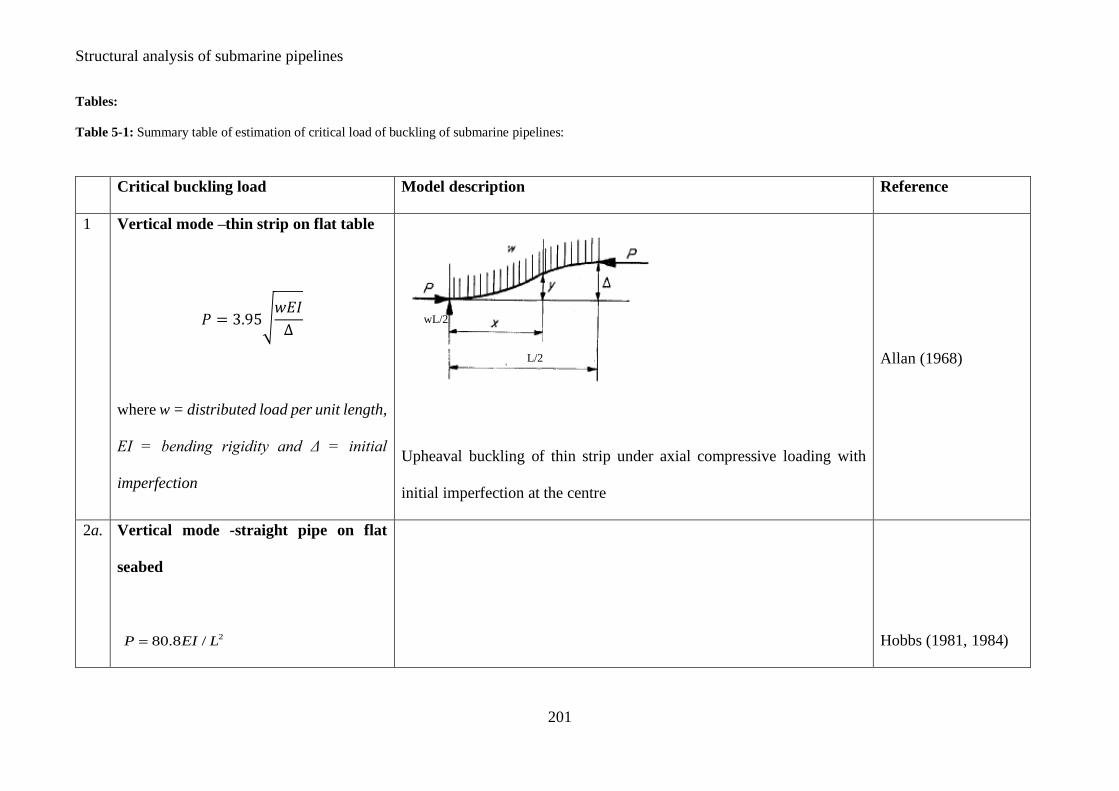
Structural analysis of submarine pipelines
201
Tables:
Table 5-1: Summary table of estimation of critical load of buckling of submarine pipelines:
Critical buckling load Model description Reference
1 Vertical mode –thin strip on flat table
𝑃 = 3.95√𝑤𝐸𝐼
Δ
where w = distributed load per unit length,
EI = bending rigidity and Δ = initial
imperfection
Upheaval buckling of thin strip under axial compressive loading with
initial imperfection at the centre
Allan (1968)
2a.
Vertical mode -straight pipe on flat
seabed
2/8.80 LEIP =
Hobbs (1981, 1984)
L/2
wL/2

Structural analysis of submarine pipelines
202
2b.
Where EI = bending rigidity and L =
length of the buckle and given by
( )125.0
2
36106856.1
=
AEw
EIL
Where A = area of the pipe, w = weight of
the pipe per unit length
Both upheaval and lateral critical buckling loads are derived and
expressed as a function of length of the buckle. It was assumed that the
bending moment and slope at the lift-off point is zero. For the lateral
mode the lateral friction force is fully mobilised and the zero slope
condition at the end is replaced by the shear force condition at the same
place.
Hobbs (1984)
Lateral mode -straight pipe on flat
seabed
22 /4 LEIP =
Where EI = bending rigidity and L =
length of the buckle and given by
𝐿 = (2.7969 × 10⁵(𝐸𝐼)3
(𝜇𝑤)2𝐴𝐸)
0.125
Where = coefficient of friction, A = area
of the pipe, w = weight of the pipe per unit
length
µwµw
µwL/2
P0-µwLs

Structural analysis of submarine pipelines
203
3a.
Vertical mode-straight pipe on flat
seabed
𝑃 = 3.96√𝑤𝐸𝐼
Δ
Where EI = bending rigidity and w =
weight of the pipe per unit length and =
height of the centre of the buckle with
length L,
𝐿 = 4.51 (𝑤𝐸𝐼
Δ)
0.25
This is an extension of Hobbs solution of straight pipe on rigid seabed
was extended to express the critical load of buckling in relation with the
buckling height
Maltby & Calladine
(1995)
D

Structural analysis of submarine pipelines
204
3b.
Vertical mode-imperfect pipe on
nonlinear seabed
𝑃 = √𝐸𝐼𝐻
Δ
where EI = bending rigidity and H =
ultimate nonlinear restoring force per
unit length and = initial imperfection
the half wave length of the buckle was
expressed as: 𝜆 = (𝐸𝐼𝐻
Δ)
0.25
The pipe was considered with initial imperfection at the centre as shown
and the soil was considered to be nonlinear.
Maltby & Calladine
(1995)
4a. Vertical mode-straight pipe on flat
seabed
The propagation load was expressed as
𝑃 = 4.029√𝐸𝐼𝑤
Δ
Croll (1997)
D
L
H
D w

Structural analysis of submarine pipelines
205
and wave length was expressed as
𝐿 = 4.427√𝐸𝐼Δ
𝑤
where w = weight per unit length and =
displacement relative to flat seabed
A perfectly straight pipe of unit weight w was resting on a flat, rigid
seabed was considered
4b.
Vertical mode-imperfect pipe on point
protrusion support
The propagation load was expressed as
𝑃 = 4.029√𝐸𝐼𝑤
Δ
and wave length was expressed as
𝐿 = 4.427√𝐸𝐼Δ
𝑤
where w = weight per unit length and =
displacement relative to flat seabed
A rigid protrusion was considered with amplitude of at the centre. With
increasing axial load the pipe will start lifting off from the support and
the length of the suspended span will be reduced from L0 to L
D
w

Structural analysis of submarine pipelines
206
4c.
Croll (1997)
Vertical mode- imperfect pipe on
continuous support
The lift-off load was expressed as
𝑃 = 3.007√𝐸𝐼𝑤/Δ
The maximum propagated buckle load
expressed as 3.478√𝐸𝐼𝑤/Δ and the
corresponding length of the buckle was
given by 𝐿 = 4.427(𝐸𝐼Δ/𝑤)1/4
The seabed profile was considered as dominant buckling mode. The
profile of the seabed and the lift-off phenomena with propagation of
buckling load was considered here and shown in the figure. With
increasing axial load the pipe starts lifting of the seabed support. Two
design load criteria had been defined and closed form solution given for
the buckling of submarine pipelines with imperfection.
w
D
Dy’’
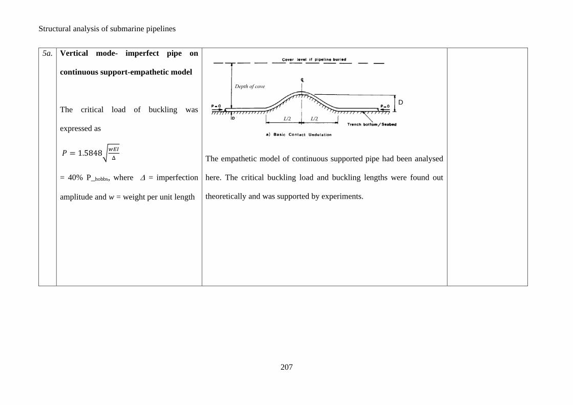
Structural analysis of submarine pipelines
207
5a.
Vertical mode- imperfect pipe on
continuous support-empathetic model
The critical load of buckling was
expressed as
𝑃 = 1.5848√𝑤𝐸𝐼
Δ
= 40% P_hobbs, where = imperfection
amplitude and w = weight per unit length
The empathetic model of continuous supported pipe had been analysed
here. The critical buckling load and buckling lengths were found out
theoretically and was supported by experiments.
D
L/2 L/2
Depth of cove

Structural analysis of submarine pipelines
208
5b
5c
Vertical mode- imperfect pipe on
isolated prop support
The critical load of buckling was
expressed as HobbsPcrP _%63=
Tran & Taylor (1996)
Vertical mode- imperfect pipe on
isolated filled-prop support
The critical load of buckling was
expressed as HobbsPcrP _%2.25=
6 Straight bar under simultaneous axial
and transverse loading
In this model a bar was considered to be straight and on elastic foundation
under axial compression.
Hetényi, 1946
D
L/2 L/2
L/2L/2
D
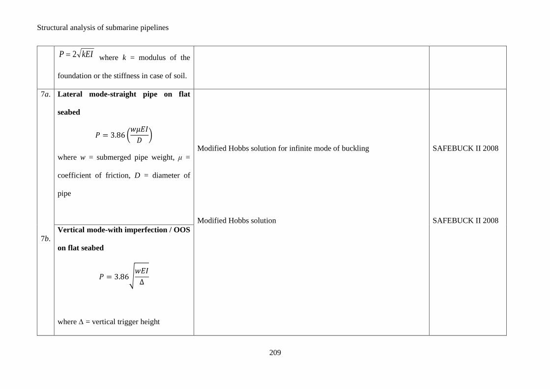
Structural analysis of submarine pipelines
209
kEIP 2= where k = modulus of the
foundation or the stiffness in case of soil.
7a.
7b.
Lateral mode-straight pipe on flat
seabed
𝑃 = 3.86 (𝑤𝜇𝐸𝐼
𝐷)
where w = submerged pipe weight, μ =
coefficient of friction, D = diameter of
pipe
Modified Hobbs solution for infinite mode of buckling
Modified Hobbs solution
SAFEBUCK II 2008
SAFEBUCK II 2008
Vertical mode-with imperfection / OOS
on flat seabed
𝑃 = 3.86√𝑤𝐸𝐼
Δ
where = vertical trigger height
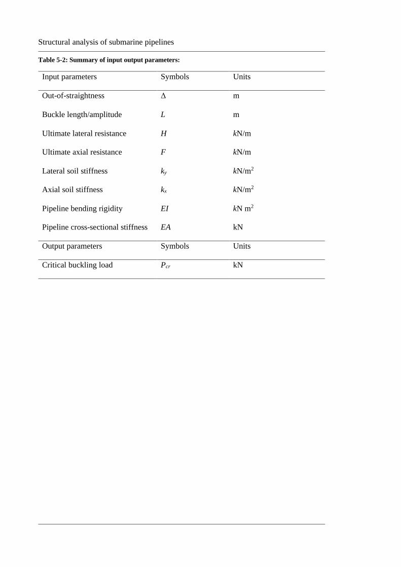
Structural analysis of submarine pipelines
Table 5-2: Summary of input output parameters:
Input parameters Symbols Units
Out-of-straightness Δ m
Buckle length/amplitude L m
Ultimate lateral resistance
Ultimate axial resistance
H
F
kN/m
kN/m
Lateral soil stiffness
Axial soil stiffness
ky
kx
kN/m2
kN/m2
Pipeline bending rigidity
Pipeline cross-sectional stiffness
EI
EA
kN m2
kN
Output parameters Symbols Units
Critical buckling load Pcr kN
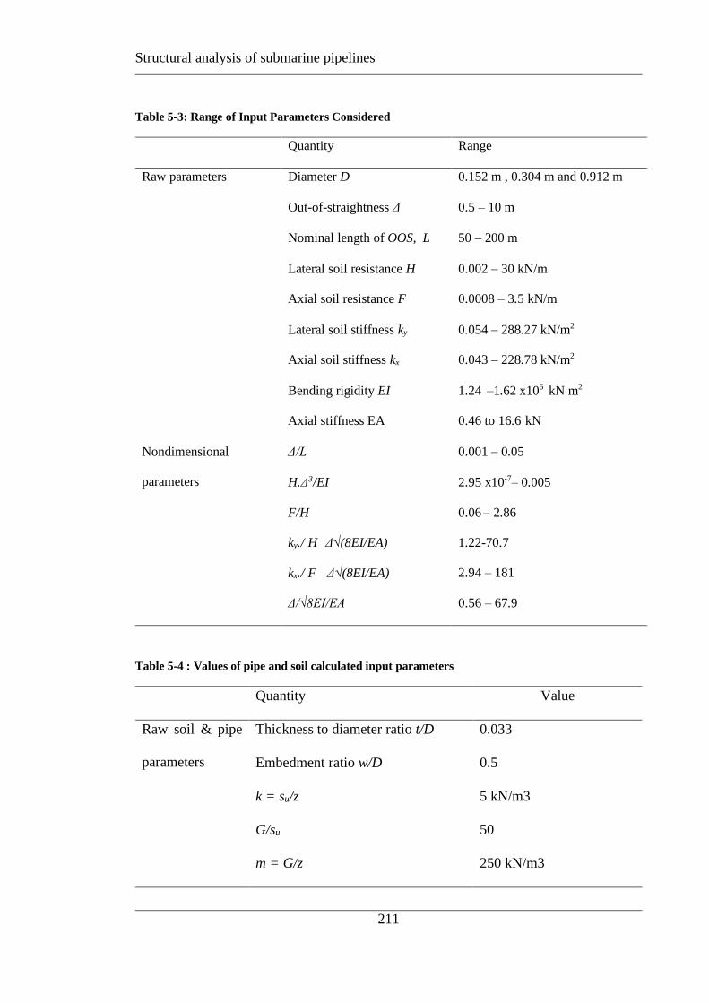
Structural analysis of submarine pipelines
211
Table 5-3: Range of Input Parameters Considered
Quantity Range
Raw parameters Diameter D 0.152 m , 0.304 m and 0.912 m
Out-of-straightness Δ 0.5 – 10 m
Nominal length of OOS, L 50 – 200 m
Lateral soil resistance H
Axial soil resistance F
0.002 – 30 kN/m
0.0008 – 3.5 kN/m
Lateral soil stiffness ky
Axial soil stiffness kx
0.054 – 288.27 kN/m2
0.043 – 228.78 kN/m2
Bending rigidity EI
Axial stiffness EA
1.24 –1.62 x10⁶ kN m2
0.46 to 16.6 kN
Nondimensional
parameters
Δ/L 0.001 – 0.05
H.Δ3/EI
F/H
ky./ H· Δ√(8EI/EA)
kx./ F · Δ√(8EI/EA)
Δ/√8EI/EA
2.95 x10⁻⁷– 0.005
0.06 – 2.86
1.22-70.7
2.94 – 181
0.56 – 67.9
Table 5-4 : Values of pipe and soil calculated input parameters
Quantity Value
Raw soil & pipe
parameters
Thickness to diameter ratio t/D 0.033
Embedment ratio w/D 0.5
k = su/z 5 kN/m3
G/su 50
m = G/z 250 kN/m3

Structural analysis of submarine pipelines
212
Figures:
Figure 5-1: Nonlinear springs considered for the three directions
Figure 5-2: Idealization of pipeline buckling model

Structural analysis of submarine pipelines
213
ζ0n+1
ζ1n+1
ζ2n+1ζ*
n
Δl
Crisfield iteration
f(ζ)=f(λ,u)
Displacement, u
2*
1
*
1 )()( ln
i
n
T
n
i
n =−− ++ L
oad
ing
p
ara
mete
r, λ
Tangential solution from ζ*n
ζ0n+1
ζ1n+1
ζ2n+1ζ*
n
Δl
Crisfield iteration
f(ζ)=f(λ,u)
Displacement, u
2*
1
*
1 )()( ln
i
n
T
n
i
n =−− ++ L
oad
ing
p
ara
mete
r, λ
Tangential solution from ζ*n
Figure 5-3: Modified RIKS method used in ABAQUS (Knappett & Madabhushi (2009))
Figure 5-4: Types of beam elements
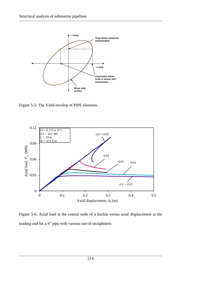
Structural analysis of submarine pipelines
214
Figure 5-5: The Yield envelop of PIPE elements
Figure 5-6: Axial load at the central node of a buckle versus axial displacement at the
loading end for a 6″ pipe with various out-of-straightness
0
0.03
0.06
0.09
0.12
0 0.1 0.2 0.3 0.4 0.5
Ax
ial
load
, P
cr(M
N)
Axial displacement, δX (m)
Δ/L = 0.05
Δ/L = 0.01
0.02
0.03 0.04
D = 0.152 m (6")
EA = 462 MNL = 50 m
H = 424 N/m
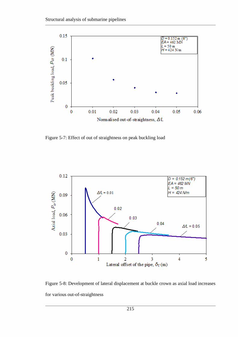
Structural analysis of submarine pipelines
215
Figure 5-7: Effect of out of straightness on peak buckling load
Figure 5-8: Development of lateral displacement at buckle crown as axial load increases
for various out-of-straightness

Structural analysis of submarine pipelines
216
Figure 5-9: Mobilised lateral soil resistance at peak load along the length of the pipeline
Figure 5-10: Comparison between initial and displaced shapes at the peak loads for
various out-of-straightness
-500
-300
-100
100
300
500
0 50 100 150 200
Lat
eral
res
ista
nce
of
the
soil,
H(N
/m)
Position, x (m)
Δ/L = 0.01
Δ/L = 0.02
Δ/L = 0.03
Δ/L = 0.04
Δ/L = 0.05
424 N/mD = 0.152 m (6")
EA = 462 MN
L = 50 m
H = 424 N/m
- 424 N/m
Δ/L = 0.05 - 0.01
-1
0
1
2
3
4
0 50 100 150 200
Lat
eral
po
sitio
n,
y(m
)
Axial position, x (m)
Δ/L = 0.01 ( initial shape)
Δ/L = 0.01 ( Shape at peak load)
Δ/L = 0.02 ( initial shape)
Δ/L = 0.02 ( Shape at peak load)
Δ/L = 0.03 ( initial shape)
Δ/L = 0.03 ( Shape at peak load)
Δ/L = 0.04 ( initial shape)
Δ/L = 0.04 ( Shape at peak load)
Δ/L = 0.05 ( initial shape)
Δ/L = 0.05 ( Shape at peak load)
D = 0.152 m (6")
EA = 462 MN
L = 50 m
H = 424 N/m
Δ/L = 0.05
Δ/L = 0.01

Structural analysis of submarine pipelines
217
Figure 5-11: Lateral offset values corresponding to peak load for various OOS
Figure 5-12: Effect of lateral limiting frictional resistance on peak load
0
0.1
0.2
0.3
0.4
0.5
0 0.01 0.02 0.03 0.04 0.05 0.06
Lat
eral
off
set
at p
eak l
oad
, δ
Y(m
)
Normalised out-of-straightness, Δ/L
Elastic limit = 0.008 m
D = 0.152 m (6")
EA = 462 MNL = 50 mH = 424 N/m
0
0.1
0.2
0.3
0.4
0 0.01 0.02 0.03 0.04 0.05 0.06
Pea
k b
uck
ling
load
, P
cr (
MN
)
Normalised out-of-straightness, Δ/L
FE results for H = 424 N/m
FE results for H = 200 N/m
FE results for H = 100 N/m
Modified Mantby & Calladine analytical solution for H = 424 N/m eq(8)
D = 0.152 m (6")
EA = 462 MN
L = 50 m
Analytical solution of Maltby & Calladine eq(3)
for H = 424 N/m

Structural analysis of submarine pipelines
218
Figure 5-13: Effect of lateral elastic slip on peak load
Figure 5-14: Comparison of normalised peak buckling loads for three cases

Structural analysis of submarine pipelines
219
Figure 5-15: Multivariate fit to computed critical buckling load without axial spring
Figure 5-16: Multivariate fit to computed critical buckling load with axial spring

Structural analysis of submarine pipelines
220
Figure 5-17: Multivariate fit to computed critical buckling load with axial spring and initial stress

Structural analysis of submarine pipelines
221

Structural analysis of submarine pipelines
222

Structural analysis of submarine pipelines
223
SUBSEA PIPELINE WALKING WITH A BI-
LINEAR SEABED MODEL
6.1 INTRODUCTION
The increasing demand of energy is not only pushing the hydrocarbon industry towards
the deeper oceans, but also pushing the operating conditions towards the high temperature
and high pressure (HT/HP) regime. Therefore, the present deepwater submarine pipelines
are being operated at HT/HP which can require special design considerations to prevent
issues related to thermal expansion, such as buckling and walking. Theories of buckling
have been developed in last two decades and are well accepted in the industry. (e.g., DNV
2007; Collberg et al. 2011 ) The so-called pipeline walking mechanism was also well
defined in last few years by various researches and by the industry projects such as
SAFEBUCK JIP (Konuk, 1998, Tørnes et. al. 2000, Carr et. al. 2006). However,
understanding the walking mechanism is becoming challenging with the increasing
complexities related to soil-pipe interaction on soft clays, particularly when considering
detailed aspects of pipe-soil interaction behaviour. Therefore, this paper will give a brief
overview of the present practices to estimate the walking of pipeline along with a
proposed expression to estimate walking in certain complex soil-pipe interaction scenario.
Once the pipeline is laid on the seabed, it is heated or cools down during operation cycles.
Due to this heat up and cool down process the pipe tends to expand and contract
respectively. These expansion and contractions are resisted by the seabed friction. When
it cools down the pipe cannot regain the original length due to the seabed resistance. This

Structural analysis of submarine pipelines
224
phenomenon is addressed in the pipeline design guidelines. In some cases the pipeline
expansion is associated with the global displacement of the pipe because the expansion
and contraction is asymmetric between the two ends, leading to a net movement of the
pipe in one direction. This is commonly known as ‘walking’ of pipeline. Walking itself
is not a limit state, but uncontrolled walking may lead to many of the critical problems,
such as, over stressing of end connectors such as spool pieces and jumpers, loss of tension
in a SCR (Steel catenary riser), increased loading within a lateral buckle and route curve
pull-out of restrained system (Carr et. al. 2006).
6.2 EXISTING WALKING MODELS
In deepwater the pipelines are often connected to the receptor facilities by SCR. This
arrangement pulls the pipeline into tension at the touch down zone. This tension at the
end of the pipeline causes a short pipe to walk under the thermal cyclic loading conditions
towards the SCR. It is assumed that there is sufficient axial friction along the length of
the pipeline to be axially stable under the highest axial riser tension (Carr et al. 2006).
Carr et al. (2006) gave the expressions for the pipeline walking under various field
conditions in work that was part of the SAFEBUCK JIP ( Collberg et al. 2011). They
expressed that, the pipeline walking behaviour of short pipelines can occur due to (1)
tension at the end of pipelines, associated with a SCR, (2) global seabed slope along the
length of the pipe, and, (3) thermal gradients along the pipeline during changes in
operating conditions. Bruton et al. (2010) added a fourth mechanism, being (4) changes
in the distribution of weight along the pipeline due to liquid hold up on shutdown. The
following section summarises the existing theories to estimate walking triggered by these
mechanisms.

Structural analysis of submarine pipelines
225
6.2.2 SCR tension
The analytical solution of pipeline walking per cycle, under the tension of SCR was given
by (Carr et al. 2006):
𝛥𝑅 =(|𝛥𝑃| + 𝑇𝑆𝐶𝑅 − 𝑓 ⋅ 𝐿) ⋅ 𝑇𝑆𝐶𝑅
𝐸𝐴 ⋅ 𝑓
(6-1)
where, ΔP is the change in fully constrained force, TSCR is the SCR tension, f is the axial
frictional force = µW′, L is the pipeline length and EA is the axial stiffness of the pipe.
The change in fully constrained force was given by:
( ) ( )1212 21)( −−−−−= Si AEAppP
(6-2)
where p is internal pressure and subscripts 1 and 2 refer to conditions before and after the
operating change, Ai is internal cross-sectional area of the pipe, ν is Poisson’s ratio of the
pipe material, As is cross sectional area of the pipe wall, E is Youngs modulus, α is
coefficient of thermal expansion and θ is operating temperature and subscripts 1 and 2
refer to conditions before and after the operating change.
The first term is the pressure term and assumed to be zero for these analyses and the
second term is the thermal term as defined earlier. Numerical analysis was also carried
out to verify the analytical solution. Analytical and numerical results were matched with
good agreement.
6.2.3 Seabed slope
The seabed slope causes the walking of pipeline under cyclic thermal loading. Carr et al.
(2006) gave an analytical model to predict the walking of an on-bottom pipeline with
sloping seabed. Figure 6-1 shows the force diagram of a pipe element resting on a seabed

Structural analysis of submarine pipelines
226
with an angle Φ. The slope of the seabed (Φ) was introduced in the previous expression
of SCR and the walking per cycle was given by:
( ) ( ) ( )
−+=
EA
LLWLWP tancossin
(6-3)
In this case there is a component of pipe weight (W′sin Φ) which acts downhill and in the
same direction of expansion. When the pipe expands up the slope, this force acts against
the expansion and when the pipe expands down the slope, this force acts with the
expansion. This affects the shape of the force envelope causes the asymmetric shape of
the force profile envelope as discussed later. FE analysis was also carried out by Carr et
al. (2006) to mutually verify the two methods. Analytical and numerical results were
matched with good agreement.
6.2.4 Thermal transients
The heat up and cool down step is needed to be considered realistically to investigate the
effect of thermal gradient on pipeline walking. The ‘hot-end’ is considered to be closest
to the well head and the ‘cold-end’ is considered to be closest to the receiver facility or
attached to riser. The pipe (and its contents) cools down uniformly over its length (when
there is no flow through the pipe) and heats up non-uniformly from one end to the other
with some gradient (due to the flow from one end to the other). Due to this reason,
expansion in one direction occurs during the heat up step, but the contraction during the
cool down step is more symmetric. A typical thermal transient model was shown in Figure
6 2(Carr et al. 2003 ). The important aspect of this phenomenon is the shape of the thermal
profile developed over time as the pipe is heated up from ambient. The hot fluid enters
the ‘hot-end’ at 0 and heat is lost to the surrounding and the fluid quickly cools down to
ambient temperature. With time the pipe is gradually heated up till the fluid is discharged
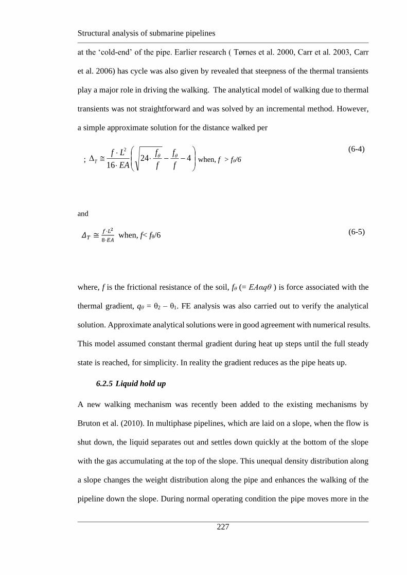
Structural analysis of submarine pipelines
227
at the ‘cold-end’ of the pipe. Earlier research ( Tørnes et al. 2000, Carr et al. 2003, Carr
et al. 2006) has cycle was also given by revealed that steepness of the thermal transients
play a major role in driving the walking. The analytical model of walking due to thermal
transients was not straightforward and was solved by an incremental method. However,
a simple approximate solution for the distance walked per
;
−−
424
16
2
f
f
f
f
EA
LfT
when, f > fθ/6
(6-4)
and
𝛥𝑇 ≅𝑓⋅𝐿2
8⋅𝐸𝐴 when, f< fθ/6 (6-5)
where, f is the frictional resistance of the soil, fθ (= EAαqθ ) is force associated with the
thermal gradient, qθ = θ2 – θ1. FE analysis was also carried out to verify the analytical
solution. Approximate analytical solutions were in good agreement with numerical results.
This model assumed constant thermal gradient during heat up steps until the full steady
state is reached, for simplicity. In reality the gradient reduces as the pipe heats up.
6.2.5 Liquid hold up
A new walking mechanism was recently been added to the existing mechanisms by
Bruton et al. (2010). In multiphase pipelines, which are laid on a slope, when the flow is
shut down, the liquid separates out and settles down quickly at the bottom of the slope
with the gas accumulating at the top of the slope. This unequal density distribution along
a slope changes the weight distribution along the pipe and enhances the walking of the
pipeline down the slope. During normal operating condition the pipe moves more in the

Structural analysis of submarine pipelines
228
downhill than uphill. Due to the settlement of the liquid down slope during shut down
process, the submerged weight reduces the uphill contraction of the pipe; the reverse
situation happens at the uphill light gas filled section of the pipe. This increases the
absolute walking downhill the slope.
Figure 6-3 shows the split length, Ls and the whole length of the pipe, L. The axial
frictional force can be found out for various split lengths as:
( ) ( )( ) 0312
12
WLL
Sc
+−−+= for
2
LLs
(6-6)
( ) ( )( ) 012
12
WLL
Sc
−−−+= for
'2
Bs LLL
(6-7)
( ) ( ) 0114
314
WLL
S sc
−−+
−++= for 'Bs LL
'Bs LL
(6-8)
Similar, to previous cases the walking rate was given by:
( )EA
XPS abcL
−=
(6-9)
where, Xab is the distance between the virtual anchor points, LB′ is the unloading virtual
anchor point, ω, is the ratio of the gas filled submerged weight to the liquid filled
submerged weight (Wg /Wo), β, is the ratio of the operating submerged weight to the
liquid filled submerged weight (W/Wo). FE analysis was also carried out to verify the
analytical solution. Analytical and numerical results were matched with good agreement.
In this paper walking due to first three mechanisms were considered for the analysis and
further study. The walking due to slope with liquid hold up could be studied separately
based on the proposed model at the end of this paper.

Structural analysis of submarine pipelines
229
6.3 MODELLING ASSUMPTIONS
The remainder of this paper describes analytical modelling supported by numerical
verification of the different types of walking behaviour. Firstly, a simple analytical
solution is described to estimate the end expansion of on-bottom pipeline resting on a flat
seabed with uniform resistance. This analytical expression is then verified with numerical
modelling. The pipe is considered to be elastic and resting on a perfectly flat seabed with
resistance expressed as friction coefficient. One end of the pipe is considered to be fixed
with other end remained free. Then the pipe is heated uniformly and the end expansion
was resisted by the friction between the pipe and the seabed. Then the numerical
verification of this model was carried out with ABAQUS (Dassault Systѐms, 2007). The
numerical analysis was carried out in both ways, once with a flat seabed with Coulomb
friction between the pipe and the seabed (rigid-plastic pipe-soil interaction, i.e.
mobilisation distance practically zero), and with nonlinear springs (elastic-plastic pipe-
soil interaction with a finite mobilisation distance) . Results of both the numerical analysis
were in good agreement with the analytical solution.
Thereafter, the existing analytical solutions for various seabed slopes, SCR tensions and
thermal transients are examined with numerical solutions. The numerical results match
with very good agreement with the existing analytical solutions. However, the elastic-
plastic response of the soil was neglected at this stage. To incorporate the mobilisation
displacement of the soil into the existing methodology to predict walking of submarine
pipelines, a new analytical solution is developed. The proposed model is then verified
with numerical results. The effect of the mobilisation displacement of the soil on the
walking behaviour of the pipeline due to seabed slope, SCR tension and thermal transients
is then checked. The results of the numerical analyses are in good agreement with the
proposed analytical model.

Structural analysis of submarine pipelines
230
A simple analytical solution is provided here to estimate the end expansion due to thermal
loading. For that solution, the following idealisations were made:
1. The pipeline remains elastic and the material properties are described by Young’s
modulus E, Poisson’s ratio υ, linear thermal expansion coefficient α .
2. The pipe can be treated as straight thin walled circular tube of thickness t and the
mean radius R (defined as ½ (outer diameter – t)).
3. The pipeline is empty and there is no internal pressure acting inside the pipeline
4. The temperature of the pipeline is considered uniform for the present analysis.
However, the actual temperature profile is complicated. The actual temperature
profile was often assumed in the literature as decaying exponentially with distance
from the hot end. This effect nonlinear temperature profile will be discussed in
detail at a later stage.
5. The left end of the pipe was considered to be fixed on the well and the right end
was considered to the free for expansion. This assumption was similar to analysis
the half length of the pipe with both ends free.
6.3.2 Analytical modelling
The pipeline is assumed to be connected to the well head and can expand freely away
from the well head. The well head is at very high temperature. When the high temperature
oil or gas starts flowing through the pipeline it is subjected to a temperature gradient, and
due to this temperature raise Δθ, it tends to expand away towards the free end. Over the
length L, the pipeline was moving away from the well head, and so the bottom exerts on
the pipe a force f, per unit length, directed towards the well head and opposing the motion.
Due to the restriction of the movement, a compressive load P develops in the pipeline.
Figure 6-4 illustrates the schematics of thermal expansion of submarine pipeline. Hence,
Structural analysis of submarine pipelines
231
the total strain can be given by the addition of the thermal strain and the strain due to the
compressive load.
𝜀𝑡𝑜𝑡𝑎𝑙 = 𝜀𝑡ℎ + 𝜀𝑐 (6-10)
The thermal strain generated due to the uniform increase in thermal gradient is given by:
𝜀𝑡ℎ = 𝛼𝛥𝜃 (6-11)
where α is the coefficient of thermal expansion of the pipeline material and Δθ is the
change in temperature.
The compressive strain can be given by:
𝜀𝑐 = − 𝑃𝐸𝐴⁄ (6-12)
Again from compatibility and equilibrium:
fdx
dP−= (6-13)
where f is the frictional resistance of the seabed can be expressed as:
WNf == (6-14)
where μ is pipe-soil of friction coefficient,W′ is the submerged weight of the pipe, and an
enhancement factor ζ, was introduced to account for wedging around the curved surface
of the pipe (White and Randolph, 2007). For simplicity the value of ζ is taken as unity.
Integrating (6-13) we get ;
1CfxP +−= (6-15)
where C1 is the constant of integration.
The axial load in the pipeline decays towards the free end. Therefore, at x = L , P = 0
fLC = 1 (6-16)
Therefore the expression of the axial load can be given by:
( )xLfP −= (6-17)
The end expansion can be expressed as;
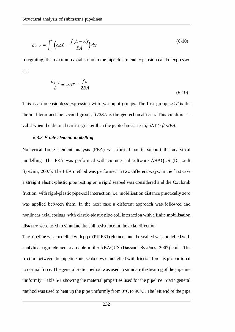
Structural analysis of submarine pipelines
232
𝛥𝑒𝑛𝑑 = ∫ (𝛼𝛥𝜃 −𝑓(𝐿 − 𝑥)
𝐸𝐴)
𝐿
0
𝑑𝑥
(6-18)
Integrating, the maximum axial strain in the pipe due to end expansion can be expressed
as:
𝛥𝑒𝑛𝑑
𝐿= 𝛼𝛥𝑇 −
𝑓𝐿
2𝐸𝐴
(6-19)
This is a dimensionless expression with two input groups. The first group, αΔT is the
thermal term and the second group, fL/2EA is the geotechnical term. This condition is
valid when the thermal term is greater than the geotechnical term, αΔT > fL/2EA.
6.3.3 Finite element modelling
Numerical finite element analysis (FEA) was carried out to support the analytical
modelling. The FEA was performed with commercial software ABAQUS (Dassault
Systѐms, 2007). The FEA method was performed in two different ways. In the first case
a straight elastic-plastic pipe resting on a rigid seabed was considered and the Coulomb
friction with rigid-plastic pipe-soil interaction, i.e. mobilisation distance practically zero
was applied between them. In the next case a different approach was followed and
nonlinear axial springs with elastic-plastic pipe-soil interaction with a finite mobilisation
distance were used to simulate the soil resistance in the axial direction.
The pipeline was modelled with pipe (PIPE31) element and the seabed was modelled with
analytical rigid element available in the ABAQUS (Dassault Systѐms, 2007) code. The
friction between the pipeline and seabed was modelled with friction force is proportional
to normal force. The general static method was used to simulate the heating of the pipeline
uniformly. Table 6-1 showing the material properties used for the pipeline. Static general
method was used to heat up the pipe uniformly from 0°C to 90°C. The left end of the pipe
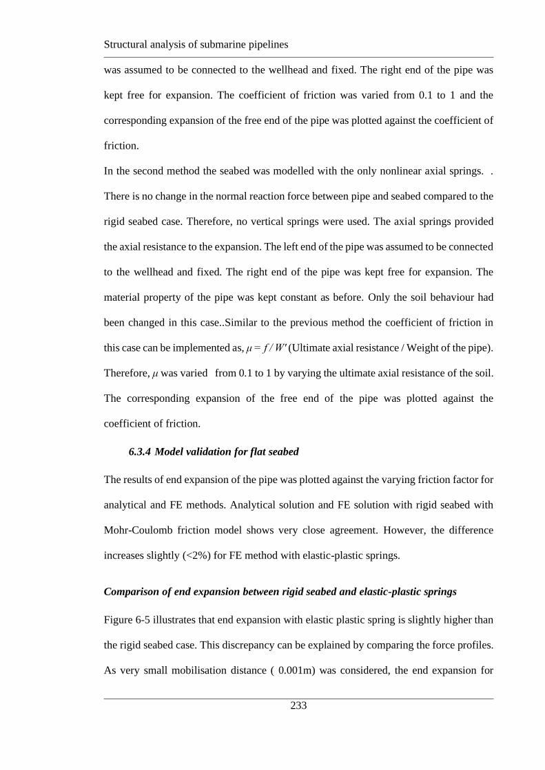
Structural analysis of submarine pipelines
233
was assumed to be connected to the wellhead and fixed. The right end of the pipe was
kept free for expansion. The coefficient of friction was varied from 0.1 to 1 and the
corresponding expansion of the free end of the pipe was plotted against the coefficient of
friction.
In the second method the seabed was modelled with the only nonlinear axial springs. .
There is no change in the normal reaction force between pipe and seabed compared to the
rigid seabed case. Therefore, no vertical springs were used. The axial springs provided
the axial resistance to the expansion. The left end of the pipe was assumed to be connected
to the wellhead and fixed. The right end of the pipe was kept free for expansion. The
material property of the pipe was kept constant as before. Only the soil behaviour had
been changed in this case..Similar to the previous method the coefficient of friction in
this case can be implemented as, μ = f / W′ (Ultimate axial resistance / Weight of the pipe).
Therefore, μ was varied from 0.1 to 1 by varying the ultimate axial resistance of the soil.
The corresponding expansion of the free end of the pipe was plotted against the
coefficient of friction.
6.3.4 Model validation for flat seabed
The results of end expansion of the pipe was plotted against the varying friction factor for
analytical and FE methods. Analytical solution and FE solution with rigid seabed with
Mohr-Coulomb friction model shows very close agreement. However, the difference
increases slightly (<2%) for FE method with elastic-plastic springs.
Comparison of end expansion between rigid seabed and elastic-plastic springs
Figure 6-5 illustrates that end expansion with elastic plastic spring is slightly higher than
the rigid seabed case. This discrepancy can be explained by comparing the force profiles.
As very small mobilisation distance ( 0.001m) was considered, the end expansion for

Structural analysis of submarine pipelines
234
rigid seabed and elastic-plastic springs matched with good agreement with the analytical
solution.
Force profile
Figure 6-6 and Figure 6-7 delineate the force profiles of rigid seabed and elastic-plastic
springs respectively for various seabed frictions. Friction factor was varied from 0.1 to 1
keeping other parameters constant. The load in the pipe reduces along the length from the
fixed end towards the free end. With increasing friction the load in the pipe also increases.
Distributed displacement
Figure 6-8 and Figure 6-9 show the distributed expansion along the length of the pipeline
due to rigid seabed and elastic-plastic springs for various resistances. Friction factor was
varied from 0.1 to 1. It is depicted that, in both the cases expansion of the pipe reduces
with increasing friction between pipe and soil. The expansion at the free end was found
out to be high due to less friction mobilisation at the end. The elastic component means
that lower friction is mobilised near the fixed end so the overall average compression
force in the pipe is less, therefore, the overall expansion is greater.
Comparison of force profiles between rigid seabed and elastic-plastic springs
Three cases were compared here with friction factors, μ =0.1, 0.5 & 1. Figure 6-10,Figure
6-11and Figure 6-12 show the force profiles of these three cases. As the elastic-slip of the
springs were chosen very small, the force profiles for first two values of friction factors
matched with good agreement. However, small deviation was observed for higher friction
factor near the fixed point. This is due to the presence of elastic-slip the load on the pipe
reduced from rigid case. This phenomenon was explained in detail later.
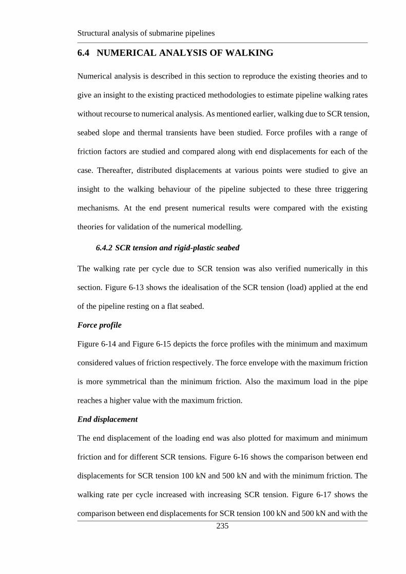
Structural analysis of submarine pipelines
235
6.4 NUMERICAL ANALYSIS OF WALKING
Numerical analysis is described in this section to reproduce the existing theories and to
give an insight to the existing practiced methodologies to estimate pipeline walking rates
without recourse to numerical analysis. As mentioned earlier, walking due to SCR tension,
seabed slope and thermal transients have been studied. Force profiles with a range of
friction factors are studied and compared along with end displacements for each of the
case. Thereafter, distributed displacements at various points were studied to give an
insight to the walking behaviour of the pipeline subjected to these three triggering
mechanisms. At the end present numerical results were compared with the existing
theories for validation of the numerical modelling.
6.4.2 SCR tension and rigid-plastic seabed
The walking rate per cycle due to SCR tension was also verified numerically in this
section. Figure 6-13 shows the idealisation of the SCR tension (load) applied at the end
of the pipeline resting on a flat seabed.
Force profile
Figure 6-14 and Figure 6-15 depicts the force profiles with the minimum and maximum
considered values of friction respectively. The force envelope with the maximum friction
is more symmetrical than the minimum friction. Also the maximum load in the pipe
reaches a higher value with the maximum friction.
End displacement
The end displacement of the loading end was also plotted for maximum and minimum
friction and for different SCR tensions. Figure 6-16 shows the comparison between end
displacements for SCR tension 100 kN and 500 kN and with the minimum friction. The
walking rate per cycle increased with increasing SCR tension. Figure 6-17 shows the
comparison between end displacements for SCR tension 100 kN and 500 kN and with the

Structural analysis of submarine pipelines
236
maximum friction. Figure 6-18 shows the comparison of end expansion over the thermal
cycle for the maximum and minimum friction with a SCR of 500 kN. The walking rate
per cycle reduces with increasing friction.
Distributed displacement
To understand the walking mechanism of the whole length of the pipe, the distribution of
displacement at various stages in the analysis were plotted. The location of selected nodes
and the SCR tension are shown in Figure 6-19. Figure 6-20 depicts the end displacements
plotted against the thermal steps along the length. It is seen that expansion and contraction
of the nodes are associated with the heat up and cool-down steps. Five heat-up and cool-
down steps were considered here. The points P0 and P643 which are on the left side of
middle point were always moved towards the SCR tension and P1359 & P2000 moved,
which are on the right side of the middle point, moved towards the right during heat up
and towards the left during cool-down. Therefore, the cumulative walking was always
towards the SCR end.
Comparison with theory
Existing analytical models have been compared with the present numerical results. Input
parameters were tabulated in Table 6-1. Figure 6-21 depicts the comparison of analytical
and numerical results for the maximum and minimum friction factors. The walking rate
is examined for a range of SCR tension. The walk per cycle is inversely proportional to
the friction factor and directly proportional to the SCR tension, keeping other parameters
remain constant. These numerical results are in good agreement with the existing
analytical solution (Carr et. al. 2006).

Structural analysis of submarine pipelines
237
6.4.3 Seabed slope and rigid-plastic seabed
Similar to the previous case, the walking rate per cycle due to seabed slope was also
verified numerically in this section. Figure 6-1 shows the idealisation of the problem
when a pipe is resting on a slope. A real slope was not modelled here, but the numerical
analysis was carried out by adjusting the direction of the gravity load to be equivalent to
the slope of the seabed.
Force profile
A seabed with 2° slope was considered here. Figure 6-22 and Figure 6-23 depict the force
profiles with the minimum and maximum friction factors respectively. The force
envelope with maximum friction was more symmetrical than with the minimum friction.
Also the maximum load in the pipe reached a higher value with the maximum friction.
End displacement
The end displacement of the loading end was also plotted for maximum and minimum
friction and for different seabed slopes. Figure 6-24 shows the comparison between end
displacements for seabed slopes of 1°, 2° and 3° and with minimum friction. The walking
rate per cycle increased with increasing slope angle..
Distributed displacement
Similar to the previous case of SCR tension, the distribution of pipe displacement at
various stages in the analysis were plotted. The locations of selected nodes and slope
idealisation were shown in Figure 6-25. Figure 6-26 depicts the end displacements plotted
against the thermal steps along the length. It is seen that, expansion and contraction of the
nodes are associated with the heat up and cool-down steps. Five heat-up and cool-down
steps were considered here. The points P0 and P477 which are on the left side of middle
point, p1000 were moved towards the downhill and points P1542 & P2000 moved,
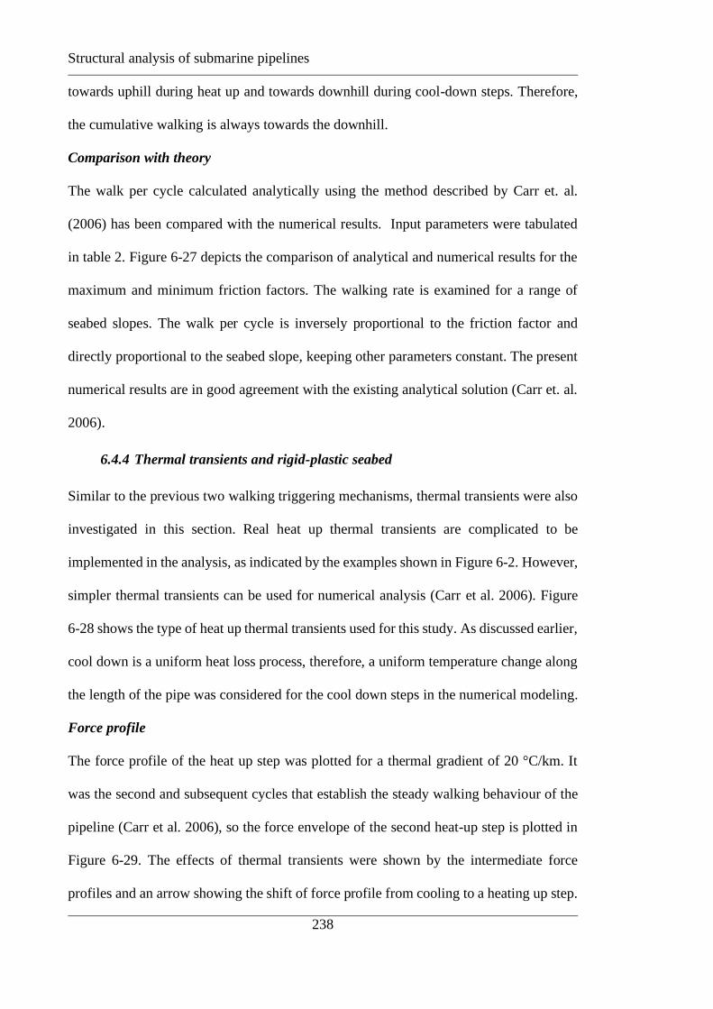
Structural analysis of submarine pipelines
238
towards uphill during heat up and towards downhill during cool-down steps. Therefore,
the cumulative walking is always towards the downhill.
Comparison with theory
The walk per cycle calculated analytically using the method described by Carr et. al.
(2006) has been compared with the numerical results. Input parameters were tabulated
in table 2. Figure 6-27 depicts the comparison of analytical and numerical results for the
maximum and minimum friction factors. The walking rate is examined for a range of
seabed slopes. The walk per cycle is inversely proportional to the friction factor and
directly proportional to the seabed slope, keeping other parameters constant. The present
numerical results are in good agreement with the existing analytical solution (Carr et. al.
2006).
6.4.4 Thermal transients and rigid-plastic seabed
Similar to the previous two walking triggering mechanisms, thermal transients were also
investigated in this section. Real heat up thermal transients are complicated to be
implemented in the analysis, as indicated by the examples shown in Figure 6-2. However,
simpler thermal transients can be used for numerical analysis (Carr et al. 2006). Figure
6-28 shows the type of heat up thermal transients used for this study. As discussed earlier,
cool down is a uniform heat loss process, therefore, a uniform temperature change along
the length of the pipe was considered for the cool down steps in the numerical modeling.
Force profile
The force profile of the heat up step was plotted for a thermal gradient of 20 °C/km. It
was the second and subsequent cycles that establish the steady walking behaviour of the
pipeline (Carr et al. 2006), so the force envelope of the second heat-up step is plotted in
Figure 6-29. The effects of thermal transients were shown by the intermediate force
profiles and an arrow showing the shift of force profile from cooling to a heating up step.

Structural analysis of submarine pipelines
239
Similarly intermediate steps of cool down are also plotted in Figure 6-30. The cool down
is typically at a uniform rate along the whole length of the pipe, leading to contraction
about the mid-line virtual anchor point. The pipeline unloads symmetrically about the
centre of the pipe as shown.
Comparison with theory
Thermal gradient applied to a pipeline have a significant effect on walking rate. . In the
model the left end is fixed and the right end of the pipe is free. Figure 6-31 illustrates the
walking rate as function of the axial friction force normalised by the constraint friction,
f* (f* = ∆P/L) at which cyclic constraint occurs, where ΔP is the fully constrained force,
and L is the length of the pipe. Three different thermal gradients were used to compare
the walking rate between existing analytical expression (Carr et. al. 2006) and the present
numerical solution. The results of the numerical analysis and the analytical solution match
with good agreement. The amount of walking is strongly influenced by the thermal
gradient, i.e. the walking rate of 30°C/km is 3 times that of 10°C/km for same f/f*.
6.5 MODELLING OF MOBLISATION EFFECT ON WALKING,
ELASTIC PLASTIC SEABED
Having verified that the numerical analysis being performed in this work is accurate,
through comparison with existing analytical solutions for pipeline walking, the numerical
analysis was extended to an elastic-plastic axial friction model.
The amount of pipeline walking is also influenced by the mobilisation displacement of
the axial friction model. A bi-linear axial response was used in FE analysis, with the
mobilization displacement being the displacement required to mobilise the full axial
resistance. The effect of mobilisation displacement on the walking behaviour of the
pipelines has been discussed by various authors (Tørnes et al. 2000, Carr et al. 2006,) and
Structural analysis of submarine pipelines
240
explored numerically and more recently analytically (Wang et. al. 2010). For example,
Wang et al. (2010) explored the effect of mobilisation displacement on long pipelines and
a ‘caterpillar-type’ locomotion was discussed. However, no analytical model for the
effect of mobilisation displacement on the walking of short pipelines has been developed
to date. This section gives a detail insight this behavior and thereafter proposes an
expression to estimate the walking rate for elastic-plastic axial friction.
6.5.2 Approach
Firstly, numerical analysis was carried out to see the effect of mobilisation displacement
on the walking. Different mobilisation displacements with same ultimate friction were
used to compare the results. The force profiles were also compared. Thereafter, an
analytical model was developed to analyse the effect of mobilisation displacement on the
force profile and hence on the walking. The next two short sections give the detail
numerical and analytical modeling to investigate the effect of mobilisation displacement
on the walking behaviour of submarine short pipelines.
6.5.3 Numerical analysis
To investigate the effect of mobilisation displacement on the walking behaviour of
submarine pipelines resting on a seabed slope, and subjected to thermal cycles, a detailed
analysis is described in this section. Three different mobilisation displacements, uutl, of
0.001 m, 0.05 m and 0.1 m were considered and are shown in the Figure 6-32. An elastic
perfectly plastic Coulomb friction model was chosen as discussed earlier. The pipe
material, size and length were kept constant as earlier cases. The seabed was considered
with a slope of, φ = 3°, and a minimum friction factor of 0.1 was considered to recover
larger end expansions, minimizing the influence of numerical errors.
The expansion at the down slope end of the pipe is plotted against cycle number for
different mobilisation displacements in Figure 6-33. This shows that with increasing

Structural analysis of submarine pipelines
241
mobilisation displacement, the walking rate reduces. The effect of mobilisation
displacement becomes prominent after the first two cycles.
The walking rate of the pipeline for various seabed slopes is also plotted for different
mobilization displacements. Figure 6-34 shows how the mobilisation displacement
affects the walking of a pipeline on a sloping seabed. To investigate the effect of
mobilisation displacement on the walking behaviour of the pipeline, the force profiles
during heat up and cool down steps are plotted for various mobilisation displacements,
uult = 0.001, 0.1, 0.2, 0.3, & 0.456m, with seabed slope, φ = 3°, and friction of 0.1 for the
same pipe considered previously (0.456m = 0.5D).
Figure 6-35 shows the force envelopes of the pipeline for heat up and cool down steps
from very low to very high mobilisation displacement. The virtual anchor points show a
very sharp edge with uult = 0.001 m, and the crown of the force envelop became parabolic
with increasing uult. The sharper peak is due to the full mobilization of the friction along
the length of the pipeline. The phenomenon was analytically explained in the following
section.
6.5.4 Analytical solution
Figure 6-36 shows the result of a force profile of a pipeline with, EA = 1.9E+10N, L = 2000
m, φ = 3°, uult = 0.456 m, ∆θ = 90°C. Only the cool down step is plotted here. Only half
of the force envelop was considered here, as this is a symmetrical case. The force profile
has been divided into four parts and the force profile for these four parts is derived to
compare the analytical and numerical results.
From the elasticity theory:
Structural analysis of submarine pipelines
242
EA
P
dx
du= (6-20)
Therefore, the equilibrium equation can be expressed as:
===
ult
passiveu
WuukF
dx
dP
(6-21)
Differentiating equation (21) and using equation (20) gives
PEAu
WP
dx
Pd
ult
2
2
2
=
=
(6-22)
where,
=
ultEAu
W2 , note, λ has two values as, λup and λdown.
The general solution of the equation can be given by:
xxBeAexP −+=)( (6-23)
The slopes of uphill and downhill can be given by:
𝑑𝑃𝑢𝑝(𝑥)
𝑑𝑥= 𝜆𝑢𝑝(𝐴𝑢𝑝𝑒𝜆𝑢𝑝𝑥 − 𝐵𝑢𝑝𝑒−𝜆𝑢𝑝𝑥)
(6-24)
and
( )x
down
x
downdowndown downdown eBeAdx
xdP −−=
)(
(6-25)
Applying the boundary conditions we get:
From point, x = xu:
WxP upu = (6-26)
Wdx
xdPup
up=
)(
(6-27)
Structural analysis of submarine pipelines
243
From point x = xd :
( ) WxLP downd −= (6-28)
Wdx
xdPdown
down −=)(
(6-29)
From point x = x0:
0)(
=dx
xdPup
(6-30)
0)(
=dx
xdPdown (6-31)
Again, the relationship between xm and L can be given by:
up
down
m
m
xL
x
=
−
(6-32)
and the distance between two unloading virtual anchor points, xd and xm can be
predicted by:
( )f
ultmd
SP
EAuxx
−=−
(6-33)
where, ∆Sf = µdownWL, the length of the unloading virtual anchor point without
mobilisation displacement is, xm, and the length of the unloading virtual anchor point with
mobilisation displacement is, xd.
Solution scheme:
Using equation (6-21) we get:
Structural analysis of submarine pipelines
244
02 x
up
up upeA
B =
(6-34)
Using equation (6-21) we get:
02 x
down
down downeA
B =
(6-35)
Using equation (6-17) we get:
( ) uupuup xxx
up
up
upee
WA
−−
=02
1
(6-36)
and, ( ) uupuup
up
xxx
x
up
up
upee
eWB
−−
=0
0
2
2
(6-37)
Using equation ((6-19) we get:
( ) ddownudown xxx
down
downdown
ee
WA
−−
=02
1
(6-38)
and, ( ) ddownudown
ddown
xxx
x
down
downdown
ee
eWB
−−
=02
2
(6-39)
Again, it can be shown that the new anchor length, X′ab is linked to the previous anchor
length Xab as:
( )mdabab xxXX −−= 2' (6-40)
Therefore, the new walk per cycle can be found out by:
( )EA
XSP abf
ult
'−=
(6-41)
Using equation (6-40), which is the rigid plastic walking rate solution, we get;
( ) ( )( )
f
ultfabf
ultSP
EAu
EA
SP
EA
XSP
−
−−
−=
2
(6-42)
Therefore, the ultimate walking per cycle for the elastic-plastic friction model can be
given by:

Structural analysis of submarine pipelines
245
∴ 𝛥𝑢𝑙𝑡 = 𝛥𝜑 − 2𝑢𝑢𝑙𝑡 (6-43)
The first term in the left hand side is the walk per cycle due to slope for a rigid plastic
seabed (i.e. without a mobilisation displacement) and the second term is the twice of the
mobilisation displacement. The same soil elastic stiffness was used for loading and
unloading cases, meaning that an increase of uult in the mobilisation displacement reduced
the walk by 2uult per cycle.
The above expression can be used to predict the walking of submarine pipelines, taking
into account the recoverable elastic component of the mobilisation displacement. Further
cases were analysed to explore how the mobilisation displacement affects the walking of
pipeline triggered by SCR tension and thermal transient.
Proposed model to estimate pipeline walking with elastic-plastic seabed
Numerical modelling was carried out to analyse the walking affected by the mobilisation
displacement for SCR tension and thermal transients, in addition to the case of seabed
slope that is analysed above. Analytical and numerical results were then compared to
verify the exactness of the proposed model, when applied to both the slope case (derived
above) and also the other cases. All the three walking mechanisms were studied here. The
material property of the pipe and the heating range were kept constant as given in Table
6-1.
The results in all cases showed that the correction by 2uult of the rigid-plastic solution
gives the correct walking rate for the elastic plastic friction model. Therefore, the solution
that is proven analytically above for the seabed slope case, is also applicable to the
thermal transient and SCR cases.
Effect of mobilisation displacement on SCR tension triggered pipeline walking
Figure 6-39 illustrates the comparison between predicted and numerical results of walk
per cycle. The mobilisation displacements were varied from 0.001 m to 0.456 m (0.5D)
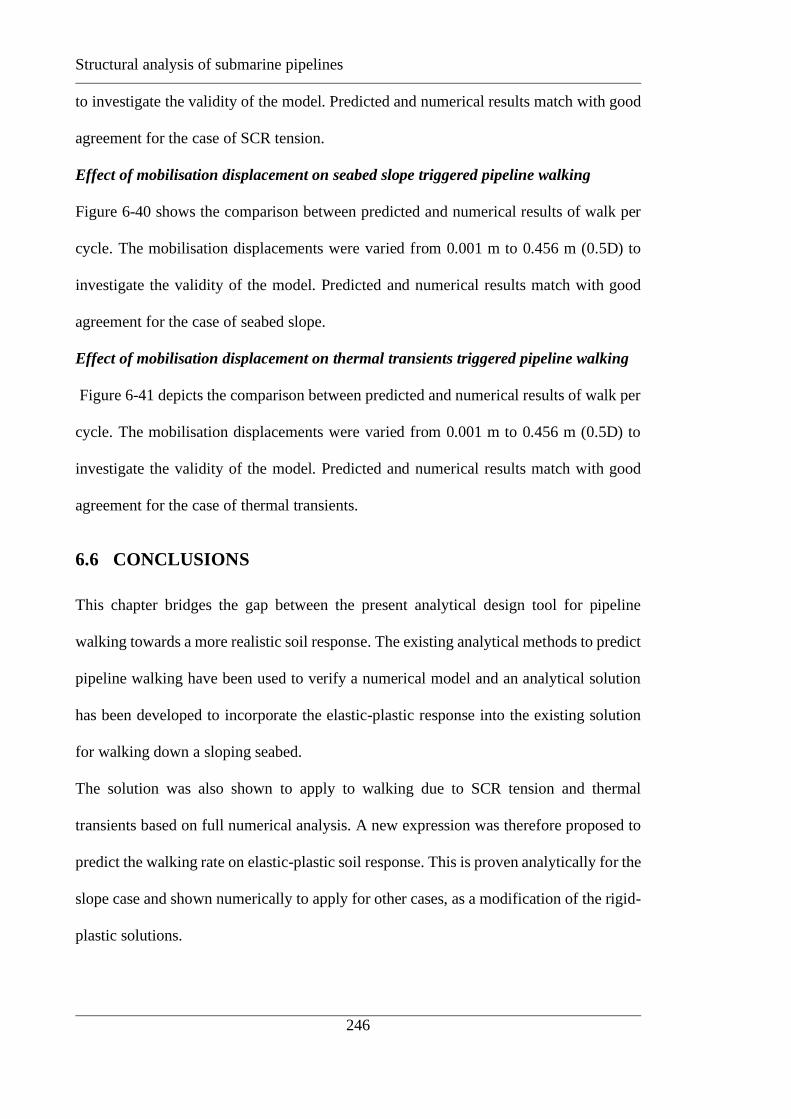
Structural analysis of submarine pipelines
246
to investigate the validity of the model. Predicted and numerical results match with good
agreement for the case of SCR tension.
Effect of mobilisation displacement on seabed slope triggered pipeline walking
Figure 6-40 shows the comparison between predicted and numerical results of walk per
cycle. The mobilisation displacements were varied from 0.001 m to 0.456 m (0.5D) to
investigate the validity of the model. Predicted and numerical results match with good
agreement for the case of seabed slope.
Effect of mobilisation displacement on thermal transients triggered pipeline walking
Figure 6-41 depicts the comparison between predicted and numerical results of walk per
cycle. The mobilisation displacements were varied from 0.001 m to 0.456 m (0.5D) to
investigate the validity of the model. Predicted and numerical results match with good
agreement for the case of thermal transients.
6.6 CONCLUSIONS
This chapter bridges the gap between the present analytical design tool for pipeline
walking towards a more realistic soil response. The existing analytical methods to predict
pipeline walking have been used to verify a numerical model and an analytical solution
has been developed to incorporate the elastic-plastic response into the existing solution
for walking down a sloping seabed.
The solution was also shown to apply to walking due to SCR tension and thermal
transients based on full numerical analysis. A new expression was therefore proposed to
predict the walking rate on elastic-plastic soil response. This is proven analytically for the
slope case and shown numerically to apply for other cases, as a modification of the rigid-
plastic solutions.
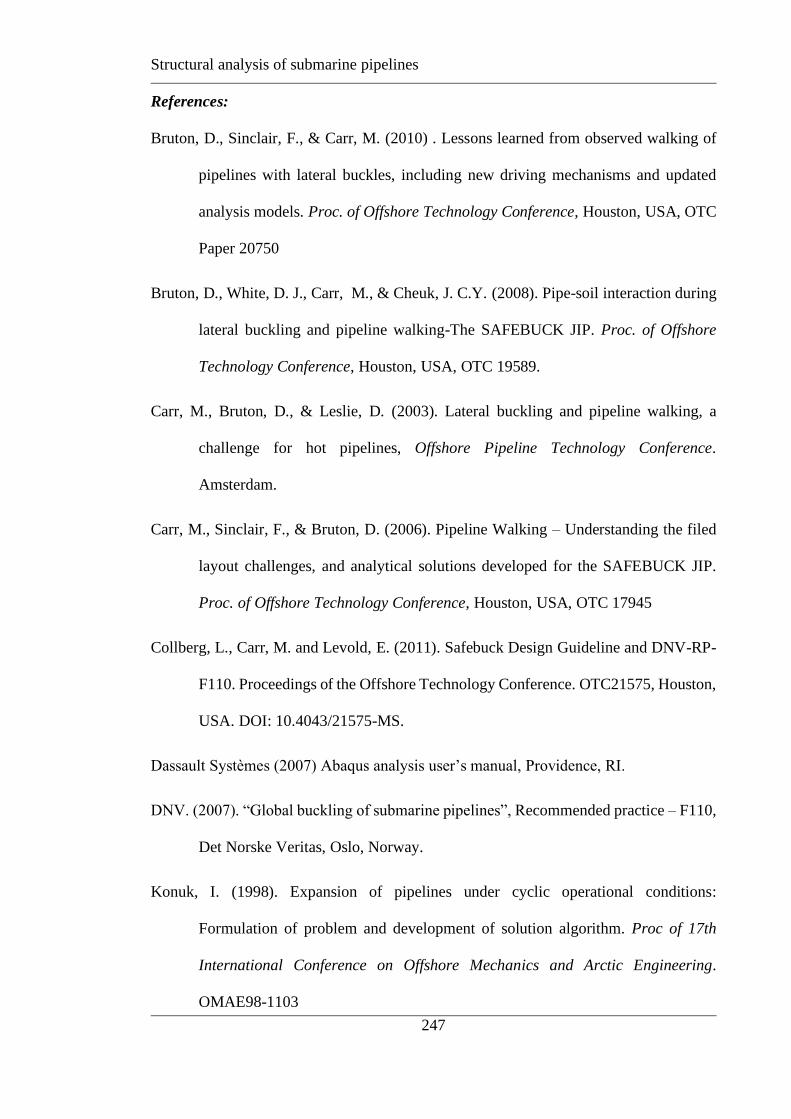
Structural analysis of submarine pipelines
247
References:
Bruton, D., Sinclair, F., & Carr, M. (2010) . Lessons learned from observed walking of
pipelines with lateral buckles, including new driving mechanisms and updated
analysis models. Proc. of Offshore Technology Conference, Houston, USA, OTC
Paper 20750
Bruton, D., White, D. J., Carr, M., & Cheuk, J. C.Y. (2008). Pipe-soil interaction during
lateral buckling and pipeline walking-The SAFEBUCK JIP. Proc. of Offshore
Technology Conference, Houston, USA, OTC 19589.
Carr, M., Bruton, D., & Leslie, D. (2003). Lateral buckling and pipeline walking, a
challenge for hot pipelines, Offshore Pipeline Technology Conference.
Amsterdam.
Carr, M., Sinclair, F., & Bruton, D. (2006). Pipeline Walking – Understanding the filed
layout challenges, and analytical solutions developed for the SAFEBUCK JIP.
Proc. of Offshore Technology Conference, Houston, USA, OTC 17945
Collberg, L., Carr, M. and Levold, E. (2011). Safebuck Design Guideline and DNV-RP-
F110. Proceedings of the Offshore Technology Conference. OTC21575, Houston,
USA. DOI: 10.4043/21575-MS.
Dassault Systѐmes (2007) Abaqus analysis user’s manual, Providence, RI.
DNV. (2007). “Global buckling of submarine pipelines”, Recommended practice – F110,
Det Norske Veritas, Oslo, Norway.
Konuk, I. (1998). Expansion of pipelines under cyclic operational conditions:
Formulation of problem and development of solution algorithm. Proc of 17th
International Conference on Offshore Mechanics and Arctic Engineering.
OMAE98-1103

Structural analysis of submarine pipelines
248
Tørnes, K., Ose, B.A., Jury, J., Thomson, P. 2000. Axial Creeping of High Temperature
Pipelines caused by Soil Ratcheting. Proc. of 19th Int. Offshore Mech. and Arctic
Eng.LA, USA. OMAE2000/PIPE-5055
Wang, Y. N., Maschner, E. A., & Hayes, R. (2010). A global migration risk to partially
constrained long pipelines subjected to localized thermal gradient cycles. Proc of
the 29th International Conference on Ocean, Offshore and Arctic Engineering,
ASME, Shanghai, China, OMAE2010-20784.
White, D. J., & Randolph, M. F. (2007). Seabed characterisation and models for pipeline-
soil interaction. International Journal of Offshore and Polar Engineering, 17(3),
193-204.
Tables:
Table 6-1: Input data used for comparison analysis:
Material properties: Parameters Units
Diameter, D 0.912 m
Length, L 2000 m
Young’s modulus, E 210 GPa
Unit weight of pipe, W′ 6.902 kN/m
Poisson’s ratio, ν 0.3
Coefficient of thermal expansion, α 12 x E-06 / ° C
Temperature rise, Δθ 90 ° C
Friction factor, μ 0.1 ~ 1
SCR tension, TSCR 100~500 kN
Seabed slope, φ 1 ~ 5 ° (angle)
Thermal gradient, qθ 10 ~ 30 °C/km

Structural analysis of submarine pipelines
249
Figures:
Figure 6-1: Force diagram of pipe element on seabed slope
Figure 6-2: Example of pipeline heat up thermal transient profiles (Carr et al. 2003)

Structural analysis of submarine pipelines
250
Figure 6-3: Schematic for walking due to liquid hold up
Figure 6-4: Idealisation of thermal expansion of submarine pipeline
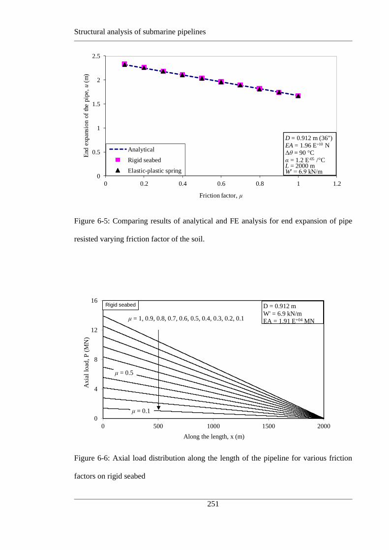
Structural analysis of submarine pipelines
251
Figure 6-5: Comparing results of analytical and FE analysis for end expansion of pipe
resisted varying friction factor of the soil.
0
4
8
12
16
0 500 1000 1500 2000
Axia
l lo
ad, P
(M
N)
Along the length, x (m)
μ = 1, 0.9, 0.8, 0.7, 0.6, 0.5, 0.4, 0.3, 0.2, 0.1
Rigid seabed D = 0.912 m
W' = 6.9 kN/m
EA = 1.91 E+04 MN
μ = 0.1
μ = 0.5
Figure 6-6: Axial load distribution along the length of the pipeline for various friction
factors on rigid seabed
0
0.5
1
1.5
2
2.5
0 0.2 0.4 0.6 0.8 1 1.2
End
exp
ansi
on
of
the
pip
e, u
(m)
Friction factor, μ
Analytical
Rigid seabed
Elastic-plastic spring
D = 0.912 m (36")
EA = 1.96 E+10 N
Δθ = 90 °C
α = 1.2 E-05 /°CL = 2000 mW′ = 6.9 kN/m
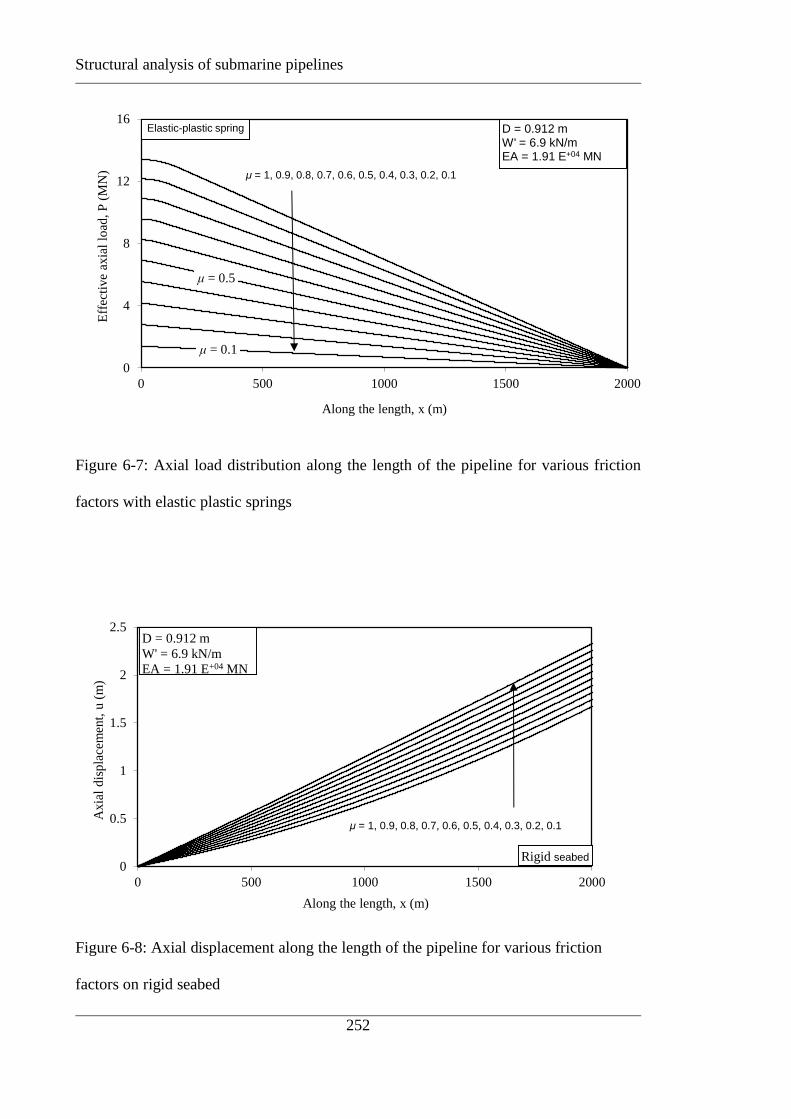
Structural analysis of submarine pipelines
252
0
4
8
12
16
0 500 1000 1500 2000
Eff
ecti
ve
axia
l lo
ad, P
(M
N)
Along the length, x (m)
μ = 1, 0.9, 0.8, 0.7, 0.6, 0.5, 0.4, 0.3, 0.2, 0.1
Elastic-plastic spring D = 0.912 mW' = 6.9 kN/mEA = 1.91 E+04 MN
μ = 0.5
μ = 0.1
Figure 6-7: Axial load distribution along the length of the pipeline for various friction
factors with elastic plastic springs
0
0.5
1
1.5
2
2.5
0 500 1000 1500 2000
Axia
l d
isp
lace
men
t, u
(m
)
Along the length, x (m)
μ = 1, 0.9, 0.8, 0.7, 0.6, 0.5, 0.4, 0.3, 0.2, 0.1
Rigid seabed
D = 0.912 m
W' = 6.9 kN/m
EA = 1.91 E+04 MN
Figure 6-8: Axial displacement along the length of the pipeline for various friction
factors on rigid seabed

Structural analysis of submarine pipelines
253
0
0.5
1
1.5
2
2.5
0 500 1000 1500 2000
Axia
l d
isp
lace
men
t, u
(m
)
Along the length, x (m)
μ = 1, 0.9, 0.8, 0.7, 0.6, 0.5, 0.4, 0.3, 0.2, 0.1
Elastic-plastic spring
D = 0.912 m
W' = 6.9 kN/m
EA = 1.91 E+04 MN
Figure 6-9: Axial displacement along the length of the pipeline for various friction factors
with elastic plastic springs
0
0.5
1
1.5
2
0 500 1000 1500 2000
Eff
ecti
ve
axia
l lo
ad, P
(M
N)
Along the length, x (m)
Rigid seabed
Elastic-plastic spring
μ = 0.1 D = 0.912 m
W' = 6.9 kN/m
EA = 1.91 E+04 MN
μ = 0.1 D = 0.912 m
W' = 6.9 kN/m
EA = 1.91 E+04 MN
Figure 6-10: Comparison of force profiles between rigid seabed and elastic-plastic
seabed for, µ = 0.1

Structural analysis of submarine pipelines
254
0
2
4
6
8
0 500 1000 1500 2000
Eff
ecti
ve
axia
l lo
ad, P
(M
N)
Along the length, x (m)
Rigid seabed
Elastic-plastic spring
μ = 0.5 D = 0.912 m
W' = 6.9 kN/m
EA = 1.91 E+04 MN
Figure 6-11: Comparison of force profiles between rigid seabed and elastic-plastic seabed
for, µ = 0.5
0
4
8
12
16
0 500 1000 1500 2000
Axia
l lo
ad, P
(M
N)
Along the length, x (m)
Rigid seabed
Elastic-plastic spring
D = 0.912 mW' = 6.9 kN/mEA = 1.91 E+04 MN
μ = 1
Figure 6-12: Comparison of force profiles between rigid seabed and elastic-plastic
seabed for, µ = 1

Structural analysis of submarine pipelines
255
Figure 6-13: Idealisation of SCR tension at the end of pipeline
Figure 6-14: Force profile with SCR Tension and for minimum friction

Structural analysis of submarine pipelines
256
Figure 6-15: Force profile with SCR Tension and for maximum friction
Figure 6-16: Comparison of end expansion for different SCR tensions with μ = 0.1
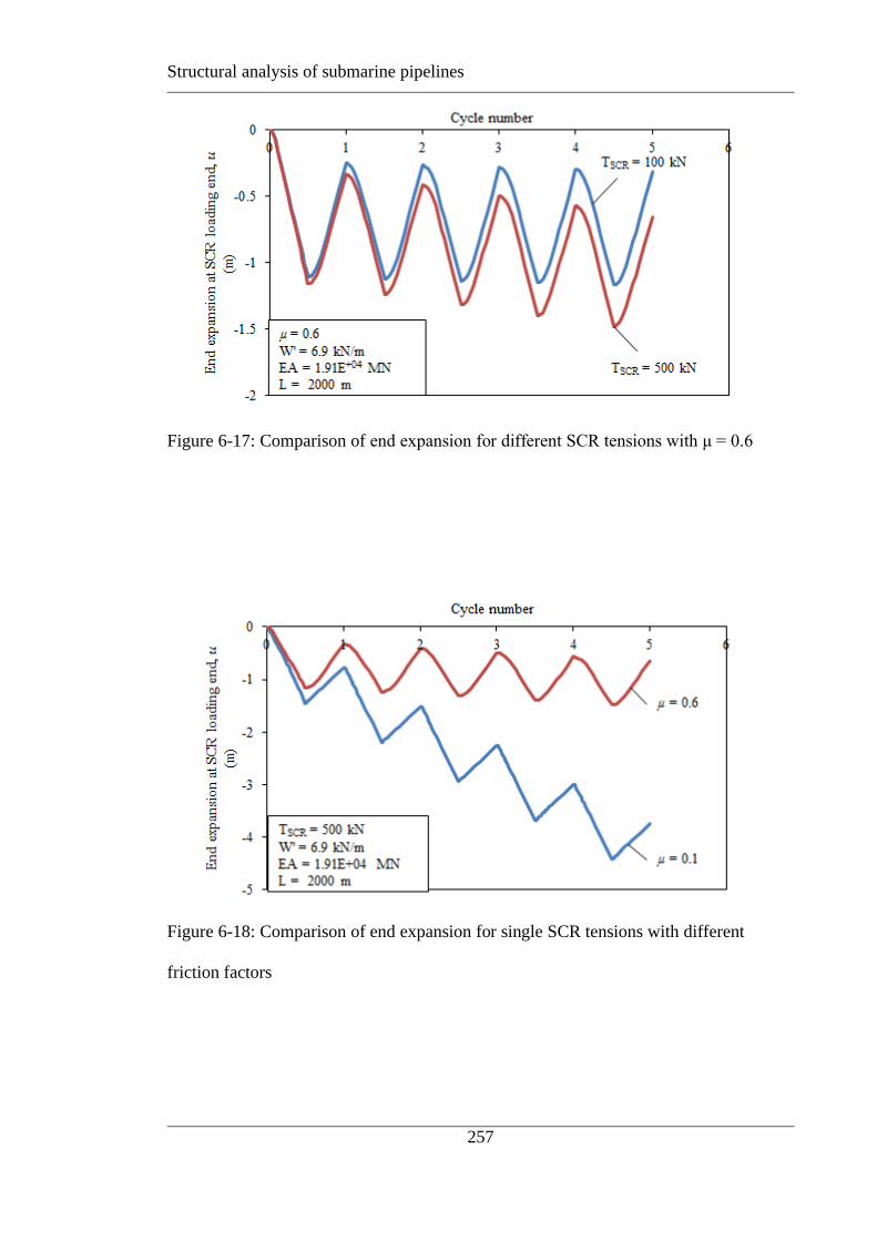
Structural analysis of submarine pipelines
257
Figure 6-17: Comparison of end expansion for different SCR tensions with μ = 0.6
Figure 6-18: Comparison of end expansion for single SCR tensions with different
friction factors

Structural analysis of submarine pipelines
258
Figure 6-19: Location of various nodes selected for distributed expansion analysis for
SCR tension
Figure 6-20: Distributed expansion at various location of the pipe for SCR tension 500
kN and minimum friction factor
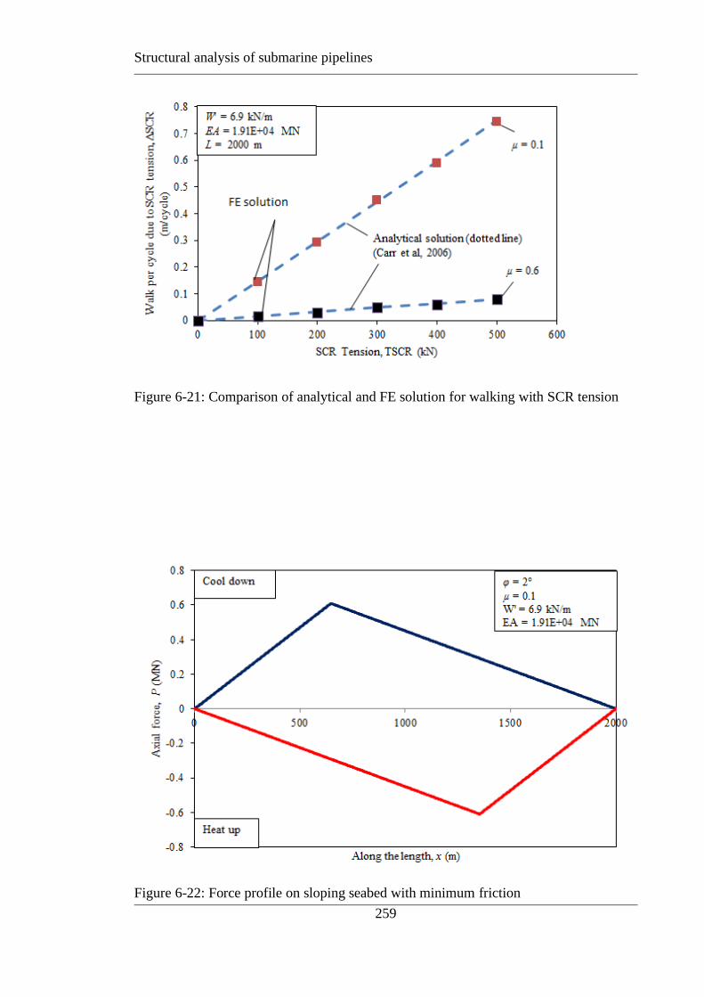
Structural analysis of submarine pipelines
259
Figure 6-21: Comparison of analytical and FE solution for walking with SCR tension
Figure 6-22: Force profile on sloping seabed with minimum friction

Structural analysis of submarine pipelines
260
Figure 6-23: Force profile on sloping seabed with maximum friction
Figure 6-24: Comparison of end expansion for different seabed slope and single
minimum friction factor
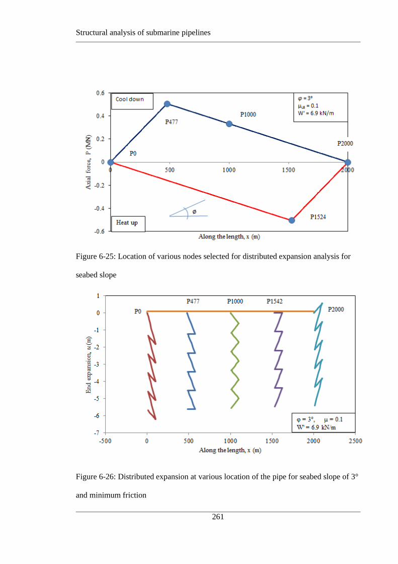
Structural analysis of submarine pipelines
261
Figure 6-25: Location of various nodes selected for distributed expansion analysis for
seabed slope
Figure 6-26: Distributed expansion at various location of the pipe for seabed slope of 3°
and minimum friction

Structural analysis of submarine pipelines
262
Figure 6-27: Comparison of analytical and FE solution for walking with sloping seabed
Figure 6-28: Example thermal transients used for the analyses
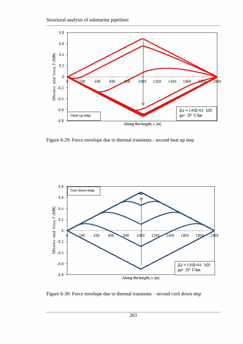
Structural analysis of submarine pipelines
263
Figure 6-29: Force envelope due to thermal transients - second heat up step
Figure 6-30: Force envelope due to thermal transients – second cool down step
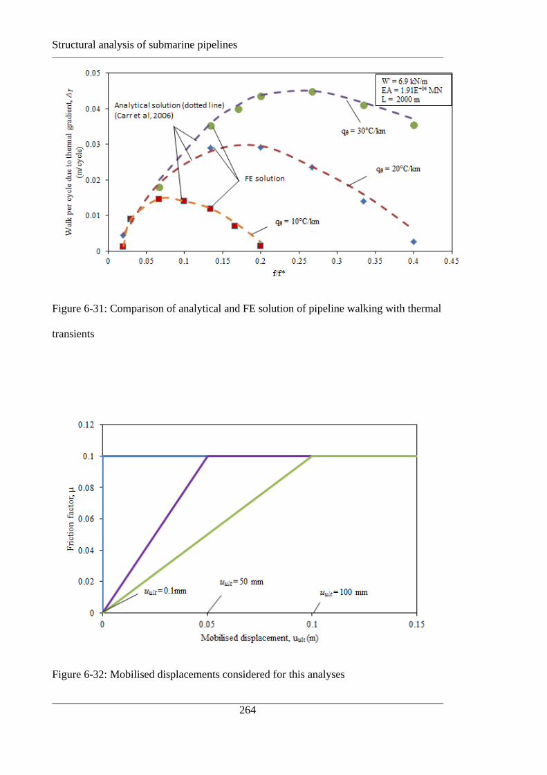
Structural analysis of submarine pipelines
264
Figure 6-31: Comparison of analytical and FE solution of pipeline walking with thermal
transients
Figure 6-32: Mobilised displacements considered for this analyses

Structural analysis of submarine pipelines
265
Figure 6-33: Effect of mobilisation displacement on a pipeline with sloping seabed and
minimum friction
Figure 6-34: The summary of effect of mobilised displacement on walking

Structural analysis of submarine pipelines
266
Figure 6-35: Comparing force profiles of various mobilisation displacements
Figure 6-36: Force profile of unloading part with mobilisation displacement

Structural analysis of submarine pipelines
267
Figure 6-37: Comparison of analytical and numerical results of pipeline walking with
mobilisation displacement
Figure 6-38: Chart to find out the effect of mobilisation displacement on pipeline
walking with a seabed slope of 3°
0
0.2
0.4
0.6
0.8
1
1.2
0 0.1 0.2 0.3 0.4 0.5
Walk
per
cycle
, ∆
t(m
)
Axial mobilisation displacement, uult (m)
Φ = 3ᵒL = 2000 mEA = 1.91E+04 MN
W' = 6.9 kN/m
µ = 0.1, 0.2, 0.3
FE results
Analytical solution(solid lines)
0
0.5
1
1.5
0 100 200 300 400 500
Wa
lk p
er
cy
cle
, ∆
φ(m
/cy
cle)
Axial mobilisation displacement, uult (mm)
φ = 3ᵒ
L = 2000 m
EA = 1.91E+04 MN
W' = 6.9 kN/m
µ = 0.1, 0.2, 0.3, 0.4, 0.5, 0.6
0.8
0.9
A
B

Structural analysis of submarine pipelines
268
Figure 6-39: Verifying the effect of mobilisation displacement on walk per cycle due to
SCR tension
Figure 6-40: Verifying the effect of mobilisation displacement on walk per cycle due to
seabed slope
0
0.1
0.2
0.3
0.4
0.5
0.6
0.7
0 0.1 0.2 0.3 0.4 0.5 0.6 0.7
Actu
al
tota
l w
alk
ing p
er
cycle
, ∆
ult
(m/c
ycle
)
Predicted walking per cycle, ∆ult (m/cycle)
∆ult = ∆SCR -2uult
W' = 6.9 kN/m
µ = 0.1
EA = 1.91E+04 MN
L = 2000 m
0
0.5
1
1.5
0 0.5 1 1.5
Actu
al
tota
l w
alk
ing
per
cycle
, ∆
ult
(m/c
ycle
)
Predicted total walking per cycle, ∆ult (m/cycle)
W' = 6.9 kN/m
µ = 0.1
EA = 1.91E+04 MNL = 2000 m
∆ult = ∆φ -2uult

Structural analysis of submarine pipelines
269
Figure 6-41: Verifying the effect of mobilisation displacement on walk per cycle due to
thermal load
0
0.01
0.02
0.03
0.04
0.05
0 0.01 0.02 0.03 0.04 0.05
Actu
al
tota
l w
alk
ing
per
cycle
, ∆
ult
(m/c
ycle
)
Predicted total walking per cycle, ∆ult(m/cycle)
10°C/km
20°C/km
30°C/km
∆ult = ∆T -2uult
W' = 6.9 kN/mµ = 0.1EA = 1.91E+04 MNL = 2000 m

Structural analysis of submarine pipelines
270

Structural analysis of submarine pipelines
271
SUBSEA PIPELINE WALKING WITH
VELOCITY DEPENDENT SEABED FRICTION
7.1 INTRODUCTION
During the operational life of a seabed pipeline, it undergoes many start-up and shut down
cycles leading to pipe-soil interaction forces that control the expansion and accumulated
movement. Accumulated axial movement due to repeated thermal cycles may lead to
global displacement, referred to as pipeline walking, and the pipeline may be designed to
buckle laterally to relieve the internal loads. The axial pipe-soil interaction forces have
significant influence on the design for walking and lateral buckling. Even though a
significant amount of experimental data on axial friction has been available (White et al.
2011), the equivalent friction coefficient for structural analysis of pipeline is often
selected without considering the significant effect of the pipeline velocity or history of
movement (Randolph et al. 2012).
In this chapter an axial pipe-soil interaction model with a velocity-dependent friction
coefficient is introduced. The model originates in the study of friction between solid
materials. It has been established in tribology that the friction coefficient that opposes the
initiation of slipping from a sticking condition is different from the friction coefficient
that opposes established slipping (Rabinowicz (1965), Moore (1975) and Bhushan (1999))
The former is typically referred to as the ‘static’ friction coefficient, and the latter is
referred to as ‘kinetic’ friction coefficient. Typically the static friction coefficient is
higher than the kinetic friction coefficient. One model to capture this behaviour assumes

Structural analysis of submarine pipelines
272
that the friction coefficient rates exponentially from the static to the kinetic value
according to the formula:
𝜇 = 𝜇𝑘 + (𝜇𝑠 − 𝜇𝑘)𝑒−𝑣𝑎 (7-1)
where μk is the coefficient of kinetic friction, μs is the coefficient of static friction, v is the
relative velocity of the surfaces, or the slip rate, and a is the rate factor (Oden & Martins.
(1985)). When a = 0, μ = μs . With increasing a, the transition between the limiting values
of friction occurs at a lower velocity as shown in Figure 7-1.
Recently a new analytical framework for estimating a velocity dependent friction
coefficient on clay soils was developed Randolph et al. 2012 and matched with the
available experimental data as:
𝐹
𝑊′= (
𝐹
𝑊′)
𝑑𝑟𝑎𝑖𝑛𝑒𝑑− [(
𝐹
𝑊′)
𝑑𝑟𝑎𝑖𝑛𝑒𝑑− (
𝐹
𝑊′)
𝑢𝑛𝑑𝑟𝑎𝑖𝑛𝑒𝑑] 𝑒
𝑙𝑛(2)(𝑇
𝑇50)
𝑚
(7-2)
where F is the frictional sliding resistance, W is the weight of the pipe, T is the time
and T50 is the time at which the frictional resistance is 50% of the undrained and drained
limits. Here, the value of T50 is close to 0.05, and m = 0.5. T can be calculated as T =
cvt/D2, where cv is the consolidation coefficient for the soil and D is the diameter of the
pipe. This model captures the observed trend for low undrained friction to be mobilised
for high speed or short duration axial pipe movements, and a high drained friction to be
mobilised for long distance slower movements.
In the present analysis a similar model to those proposed by White et al. (2011) and
Randolph et al. (2012) has been applied to the resistance between a pipe and the seabed
during axial pipeline motion. The parameter μk is replaced by μLB, the apparent
coefficient of friction in undrained conditions and μs by μUB, the coefficient of friction in

Structural analysis of submarine pipelines
273
drained conditions. The form of the relationship has been kept constant, but the
exponential index was recast slightly as :
𝜇 = 𝜇𝐿𝐵 + (𝜇𝑈𝐵 − 𝜇𝐿𝐵)𝑒−𝜆
𝑣𝑣50 (7-3)
where the term v50 is the velocity at which the friction factor lies 50% of the way between
the limiting values. The velocity parameter, v50, depends on the drainage behaviour of the
soil and can be estimated from laboratory tests and varies from soil to soil. Figure 7-2
shows the relation between friction factor and velocity given by equation (7-2); this model
is referred to throughout this paper as the friction rate model. The position of v50 is
indicated in the diagram. The constant λ is equal to ln 2 (0.693) because e-ln2 = 0.5.
7.2 OBJECTIVE
The present design practice for analysing pipeline walking behaviour was discussed in
the previous paper, and the conventional elastic-plastic pipe-soil response was analysed.
In conventional analyses, the rate of thermal loading during operating cycles is not
considered within the analysis. However, the velocity varies with position along the
pipeline and with time during the startup or shutdown event. Recently, it has been
recognised that the sliding resistance between a pipe and the seabed varies with velocity
due to drainage effects ( White et al. (2011) and Randolph et al. (2012)) but to date this
has not been incorporated in any structural modelling of pipeline walking.
This paper develops a numerical model in which dynamic walking behaviour is studied
in detail. A velocity-dependent friction model is implemented in commercial software
ABAQUS and validated via single element and simple (flat seabed) pipeline cases. This
model is then used for a parametric study exploring walking driven by seabed slope and
SCR end tension. The effect of differing rates of heating and cool-down on walking

Structural analysis of submarine pipelines
274
behaviour are also investigated. Finally, the potential to express the velocity-dependent
response in terms of an equivalent friction is explored.
7.3 VELOCITY DEPENDENT PIPE-SOIL RESISTANCE
It has been recognised that the sliding resistance between a pipe and the seabed varies
depending on the velocity of movement. This is principally due to the effects of
consolidation and drainage.
To establish more realistic pipe-soil interaction White & Cathie (2010) and Hill et al.
(2012) performed the time dependent pipe-soil friction model tests. The tests revealed
that axial resistance is strongly influenced by the rate of movement and the pause period
between the movement events. The higher peak values of friction factors were associated
with longer waiting periods between axial sweeps and the lowest residual values were
associated with the fastest rates of shearing.
7.3.1 Existing data
The effect of velocity on interface shear strength is shown in Figure 7-3 (Hill et al.,2012).
The response of fine-grained soil during shearing varies between fully drained and fully
undrained conditions across a wide range of velocities ( White and Cathie (2010)). Data
from previous research by Hill et al. (2012) and Steelfelt (1993) have been summarised
in the figure, with τres the mean shear stress on the pipe surface curing steady motion at
velocity v and σ′no the initial normal effective stress. These results are all from clay
samples with an over consolidation ratio (OCR) of 1, where the OCR is the ratio of the
previous maximum effective stress to the current effective stress. A value of OCR = 1 is
typical for soft clay seabeds, particularly when disturbed and then loaded by the process
of laying and then operating a pipeline. For a high velocity, partially or fully undrained
conditions will prevail, and positive or negative excess pore pressure will be generated
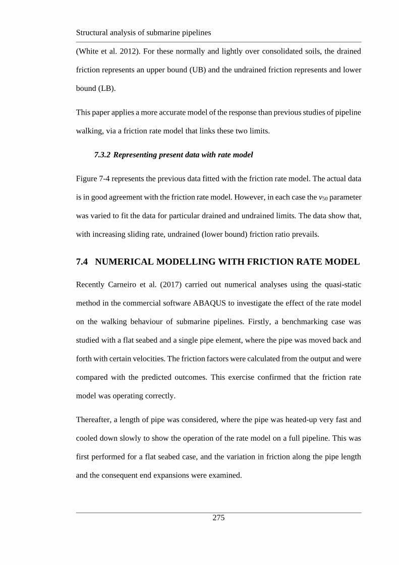
Structural analysis of submarine pipelines
275
(White et al. 2012). For these normally and lightly over consolidated soils, the drained
friction represents an upper bound (UB) and the undrained friction represents and lower
bound (LB).
This paper applies a more accurate model of the response than previous studies of pipeline
walking, via a friction rate model that links these two limits.
7.3.2 Representing present data with rate model
Figure 7-4 represents the previous data fitted with the friction rate model. The actual data
is in good agreement with the friction rate model. However, in each case the v50 parameter
was varied to fit the data for particular drained and undrained limits. The data show that,
with increasing sliding rate, undrained (lower bound) friction ratio prevails.
7.4 NUMERICAL MODELLING WITH FRICTION RATE MODEL
Recently Carneiro et al. (2017) carried out numerical analyses using the quasi-static
method in the commercial software ABAQUS to investigate the effect of the rate model
on the walking behaviour of submarine pipelines. Firstly, a benchmarking case was
studied with a flat seabed and a single pipe element, where the pipe was moved back and
forth with certain velocities. The friction factors were calculated from the output and were
compared with the predicted outcomes. This exercise confirmed that the friction rate
model was operating correctly.
Thereafter, a length of pipe was considered, where the pipe was heated-up very fast and
cooled down slowly to show the operation of the rate model on a full pipeline. This was
first performed for a flat seabed case, and the variation in friction along the pipe length
and the consequent end expansions were examined.
Structural analysis of submarine pipelines
276
The rate model was then used to show the difference in walking behaviour for various
driving mechanisms. The effect of the rate model on walking due to SCR tension, seabed
slope and thermal transients was studied in detail. In each case an attempt has been made
to express the complex outcomes from the rate model in a simpler way by plotting the
force profiles and walking rates and thereby comparing them with the response for
conventional friction models based on the undrained and drained friction limits.
Finally, a parametric analysis was carried out to evaluate the walking rate for different
rate models. Once the walking rate was derived from the numerical analysis, a back
calculation was made to find out the equivalent velocity-independent friction factor for
each of case. The aim of this step is to illustrate to what extent the velocity-dependent
friction behaviour can be mimicked in a conventional analysis using a single friction
coefficient.
7.4.1 Non-dimensional analysis
The results of numerical analysis were synthesised in non-dimensional manner. Various
dimensionless groups were identified as follows:
Relative duration of operations
Firstly, the relative rate of heating and cooling was considered with a dimensionless time
parameter, Thc is defined as:
C
Hhc
t
tT = (7-4)
where, tH is the time of heating and tC is the time of cooling. Throughout this analysis Thc,
was considered to be 0.01 unless otherwise specified. The heating of the pipe is rapid,
reflecting a sudden flooding with product, whereas the cooling is slower, reflecting heat
loss through conduction into the surrounding soil and water.
Structural analysis of submarine pipelines
277
Characteristic and Dimensionless velocity
Another dimensionless group was formed by dividing the characteristic velocity of the
pipe expansion by v50. This group is essentially the ratio between (twice) the velocity of
the ends of the pipe if the thermal expansion is unconstrained, and the characteristic
velocity of the soil drainage.
The characteristic pipe velocity, Vp is given by:
( )
CH
ptt
LV
=
m/s (7-5)
where α is the coefficient of thermal expansion of the pipe material, ∆θ is the temperature
change, L is the length of the pipe. In most of these analyses, values of the parameters
were maintained at α =12.0E-06 /°C, ∆θ = 90°C, L = 2000 m, tH = 10 s and tC = 1000 s.
These give Vp = 0.00216 m/s. Although the absolute values of tH and tC are impractically
small, the corresponding dimensionless velocities span the range between drained and
undrained conditions for the particular values of v50 adopted.
The dimensionless velocity is therefore:
( )
50
/
v
ttL CH =
(7-6)
To vary , the soil property v50 was varied.
Characteristic strain
The characteristic strain in the pipeline, c, is the ratio between the total pipe weight, WL,
which controls the force profile in the pipe through the mobilised friction coefficient, and
the axial stiffness of the pipe, EA, thus
Structural analysis of submarine pipelines
278
EA
L'Wc = (7-7)
Through most of this paper the dimensionless strain was kept constant at 0.00072, based
on W′ = 6.9 kN/m, L = 2000 m and EA = 1.9E+10 N. This axial stiffness corresponds to a
steel pipe of outer diameter, D = 0.912 m (36″) and wall thickness, t = 0.033 m.
The characteristic strain is related to the mechanical strain that shortens the pipeline when
the friction is full mobilised. In this case, ignoring the small central region where the
limiting friction is not fully mobilised, for a constant friction coefficient , the force at
the mid-point of the pipe is WL/2 and the average force along the pipe is WL/4. The
consequent strain in the pipe is c/4 and the overall mechanical shortening is cL/4, or
cL/8 at each end relative to the centre. This mechanical shortening counteracts the ‘free
pipe’ thermal expansion at each end that is given by ()L/2.
7.4.1 Benchmarking case - single element test
Figure 7-5 illustrates the model used for the benchmarking case with the friction rate
model in ABAQUS . A single element beam model, one metre in length, was used for the
pipe and a rigid surface element was used for the seabed. Gravity load was applied to
settle the pipe on the seabed and then dynamic steps were used to pull the pipe with
specified velocities.
Two cases A10 and A100 were studied with different decay factor a = 10 and 100 s/m
resulting in values for v50 = 0.069 m/s and 0.0069 m/s respectively, together with
mobilisation displacement for the elastic-plastic response of the pipe-seabed interface of
uult = 0.01 m. The mobilised friction factor, μ was extracted from the results of the
analyses as μ = τ /σ′, where τ is the shear stress in the axial direction and σ′ is the normal
pressure on the seabed. The numerical results were then compared with the theoretical

Structural analysis of submarine pipelines
279
model response. A pipe with diameter, D = 0.912 m (36) with D/t = 25 and axial stiffness,
EA = 19100 MN was used for this analysis. A yield stress, σy = 410 MPa was also
specified for the pipe element, but the yield stress was not reached in this analysis and the
pipe remained elastic throughout.
For the soil, throughout this study, an undrained friction factor, representing a lower
bound (LB), of μUD = 0.1 was adopted, along with a drained friction factor, representing
an upper bound (UB) of μD = 0.6. The input velocities and the rate (and rate, v50) factors
were tabulated in Table 7-1. The velocity was slowly ramped up to 10 m/s and then
reduced by a factor of 10 in six steps to 0.00001 m/s and then again increased back to 10
m/s for both cases. Every time step was of equal duration (10 s) for simplicity. Figure 7-6
shows the resulting velocity regime.
Figure 7-7 shows the comparison between analytical model and the numerical results.
The velocity was varied from a very high value of 10 m/s to a low value of 0.00001 m/s
and then again increased from the low value to the high value. By doing this a wide range
of velocities were covered in order to judge the accuracy of the friction rate model. The
calculated equivalent friction factor matches closely with the theoretical expression,
confirming correct operation of the model.
At very large pipe velocities, such as those considered here, viscous effects become
important, and the friction coefficient will increase again as the shear strength of clay
depends on the rate of shearing
7.4.2 Benchmarking case – 2 km pipeline on flat seabed (β= 0)
For the second benchmarking case the same input parameters were chosen for a 2 km
long pipeline resting on a flat seabed. The pipe is assumed to have free ends, therefore, a
boundary condition of zero force applies.
Structural analysis of submarine pipelines
280
The times of heating and cooling were varied to investigate the effect of velocity and the
resulting velocity dependent friction on the end expansion of the pipeline. For this
analysis the dimensionless time Thc was maintained at 0.01, with the time of heating taken
as tH = 10 s, and hence the time of cooling was tC = 1000 s, with 5 full cycles simulated
starting with heating by 90° and then cooling by the same amount. A waiting time of twait
= 100 s was introduced following each heating or cooling stage to stabilise the unbalanced
forces present at the end of the very fast heating. For these input parameters and taking
v50 as 0.0693 m/s, the dimensionless velocity is = 0.0311.
The dimensionless characteristic strain parameter, εc was kept constant at 0.00072. Cases
using the drained (UB) and undrained (LB) friction factors as well as the rate model were
used. The results of all of these models are compared in the following sections. Two key
outputs are the end movements and the mobilised friction at the free ends of the pipeline
which are plotted against time. In addition, the force envelopes and the mobilised friction
along the length of the pipeline at the end of each change in temperature are also compared.
Figure 7-8 shows the end displacement of the pipe at x = 0 over the five heating and
cooling cycles for different friction models, reflecting the net expansion of the pipeline.
Firstly the end displacements are plotted for both drained and undrained friction factors.
The drained friction factor leads to smaller expansion of the pipe and a lower cyclic range,
reflecting the greater mechanical compression in response to the expansive thermal
strains, and the greater mechanical extension in response to the contraction. After the first
expansion the cyclic response repeats exactly.
The end expansion in response to the rate model is superimposed on the plot. The
response matches the drained solution during cool down – when the velocity is slow, and
the mobilised friction is close to the drained – and matches the undrained solution at heat
Structural analysis of submarine pipelines
281
up step – when the velocity is fast. These effects are also evident in the effective friction
at the end of the pipe, which is shown in Figure 7-9.
Figure 7-10 shows the comparison of force profiles between the drained, undrained and
rate models and Figure 7-11 shows the corresponding variation in mobilized friction
along the pipe. The friction profile was calculated by dividing the change in force along
the length dP/dx, by the unit weight of the pipe, W′.
These results show that during the slow cool down process the mobilised friction along
the entire length of the pipeline is similar to the drained value, resulting in an almost linear
variation in force. However, the more rapid heat up process causes velocities in the range
over which the friction varies significantly. The result is a non-linear variation in force
along the pipe. The profile matches the undrained friction case near the fast-moving pipe
ends, but the mobilised friction is higher near the center of the pipe, where the velocity is
lower.
Figure 7-12 shows an enlarged view of the central portion of the pipe during cool down
steps. The drained (UB), undrained (LB) and rate model created a zig-zag portion at the
center of the pipe. These are due to the presence of mobilisation displacement in the
elastic-plastic pipe-seabed frictional interface model used in ABAQUS. During cooling
down and heating up the pipe experiences inward and outward displacements of the pipe
respectively. However, because of the previous heating cycle, the cooling stage does not
give sufficient inward displacement near the center of the pipe to reverse the sense of the
friction.
7.4.3 Walking due to SCR tension
A comparative study is presented in this section to investigate the effect of the rate model
on steel catenary riser (SCR) tension. The force profiles, mobilised friction (expressed as

Structural analysis of submarine pipelines
282
the ratio of change in force along the length to the weight of the pipe) and walking rates
were compared between velocity independent and velocity-dependent friction for
particular non-dimensionalised terms ψ = 0.0311, Thc = 0.01 and c = 0.00072. For this
case SCR tension of 500 kN at x = 0 was considered, maintaining a free end at x = 2000 m.
Force profile
Figure 7-13 shows the comparison of force envelopes for drained (UB), undrained (LB)
and rate friction models. The force profiles of the drained and rate models at the cool
down step are comparable. However, the maximum force reached with the rate model is
slightly lower than the drained value. This was due to the selection of total time for the
cool down step. The maximum value reached with the rate model in the heating step was
higher than the undrained value. However, the slopes of the undrained and rate models
match very closely towards the free end of the pipe.
Friction profile
Friction profiles are plotted in Figure 7-14. Mobilised friction was calculated from the
force profile as previously by (dP/dx)/W′. The drained (UB) and undrained (LB) values
were 0.6 and 0.1 respectively and the resulting force profiles are shown by the solid lines.
However, the results of the rate model match closely with the drained response over most
of the pipe length for the cool down step but with the undrained response towards each
end of the pipe for the heating step.
Walking rate
The walking rate over the five cycles is compared for the drained (UB), undrained (LB)
and rate model in Figure 7-15. For the first cycle the walk rate was similar for all the
friction. However, the effects of friction factors were more prominent after the second

Structural analysis of submarine pipelines
283
cycles due to the stabilisation of the model from the second step onwards. The walking
rate with the undrained friction was much higher than for the drained case while results
for the rate model fall in between the drained and undrained responses.
7.4.4 Walking due to seabed slope
A comparative study is presented in this section to investigate the effect of the rate model
on seabed slope with an angle Φ. Similar to previous section force profiles, mobilised
friction and walking rates were compared for drained, undrained and rate models keeping
ψ = 0.0311, Thc = 0.01 and c = 0.00072. For this case a seabed slope angle of Φ = 3° was
considered, with the lower end at x = 0.
Force profile
Force profiles for drained (UB), undrained (LB) and rate models are compared in Figure
7-16 for the seabed slope case. The maximum force reached with the rate model during
cool down is slightly lower than for the drained case. The maximum compressive force
reached with the rate model in the heating step was higher than for the undrained case.
However, the slopes for the drained and rate models match closely towards the free end
of the pipe.
Friction profile
Figure 7-17 compares friction profiles (strictly ratios of force gradient to pipe weight) for
the drained (UB), undrained (LB) and rate models with a seabed slope. The friction values
for drained ( = 0.6) and undrained ( = 0.1) respectively are shown by the solid lines
and corresponding results for the rate model by dashed lines. Results of the rate model
match closely with the drained case over most of the pipe length, especially over the
Structural analysis of submarine pipelines
284
central part, for the cool down step but more closely with the undrained case towards each
free end for the heating step.
Walking rate
Similar to the previous case of SCR tension, the walking rate over the five cycles is
compared for drained (UB), undrained (LB) and rate models in Figure 7-18. For the first
cycle the walk rate was similar for all the friction models. However, the effects of friction
factors became more prominent during subsequent cycles due to stabilisation of the model
from the second step onwards. The walking rate with the undrained (LB) friction was
much higher than for the drained case while results for the rate model falls between the
drained and undrained responses.
7.4.5 Walking due to thermal transients
A comparative study has been carried out in this section to investigate the effect of the
rate model on walking triggered by thermal transients. For this case the pipe is assumed
to have a constant initial temperature of 10°C initially, and at the end of each cool down.
However, during heating a constant temperature gradient of 10°C/km (hottest at x = 0) is
assumed. The same dimensionless parameters of ψ = 0.0311, Thc = 0.01 and c = 0.00072
were adopted.
Walking rate
Figure 7-19 shows the comparison of walking rate for drained (UB), undrained (LB) and
rate models for the thermal transient case. The walking rates over five cycles are presented
for the cold end of the pipe (x = 2000 m). The dotted line represents the displacements
with the rate model, whereas the solid lines represent the drained and undrained friction
cases. The walking rate with undrained friction was higher than for drained friction and
that with the rate model falls between these cases.

Structural analysis of submarine pipelines
285
Force profile
The force profiles with the rate model are shown in Figure 7-20 for the thermal transient
case with the rate model. Force envelopes from the second heat up and cool down cycles
till the fifth cycle are plotted, and show that the force profile stabilized after the second
cycle.
7.4.6 Distributed displacements with rate model
The distributed displacement at various locations along the pipe are presented here to
illustrate the total walking behaviour of the pipeline with the rate model, for the cases of
an applied SCR tension, a seabed slope and thermal transients.
SCR tension
Figure 7-21 shows the axial displacement at various points along the length of the
pipeline, for the case of SCR tension of 500 kN applied at x = 0. Other results for this
case have been presented previously. Towards each end of the pipeline the displacements
cycle between outward during heating and inward during cooling. However, there is a net
cumulative (negative) displacement towards the applied SCR tension. This is most
evident at the centre of the pipeline where the displacements are negative during both
heating and cool down steps.
Seabed slope
Figure 7-22 shows the plot of axial movement along the length of the pipe with a seabed
slope, β = 3° as indicated in the plot. The pattern of displacements is very similar to that
for the SCR tension case, but with larger net downhill (negative) cumulative
displacements. During each heating and cool down step the displacements at the pipeline

Structural analysis of submarine pipelines
286
centre are negative and even at x = 1500 m the net heating displacements become slightly
negative after the first cycle.
Thermal transients
Figure 7-23 shows the cyclic displacements along the length of the pipe for a thermal
transient of 10 °C/km, as indicated in the plot. The cyclic displacements follow a similar
pattern to those with no thermal gradient, being outward from the pipeline centre during
heating, and inward during cool down. The main difference relative to the previous two
cases is there is much less net walking of the pipeline. At the centre, x = 1000 m, small
cyclic displacements occur due to the additional heating for x < 1000 m compared with
x > 1000 m, but with barely discernible accumulation over successive cycles.
7.5 PARAMETRIC STUDY EXPLORING EQUIVALENT
FRICTION
A parametric study was carried out to investigate the effect of dimensionless velocity on
the walking rate of the pipeline, to establish an approach to define an equivalent single
value of friction when using the rate model. Input parameters are tabulated in Table 7-2.
The midpoint velocity of the friction rate model was varied from v50 of 0.0069 m/s to
69.31 m/s (see Figure 7-24). This range allowed simulations to cover both extremes of
the friction model. Non-dimensional parameters and c (which was kept constant) are
shown in

Structural analysis of submarine pipelines
287
Table 7-3. All three pipeline walking mechanisms were studied in the following section
to understand how the walking rate is affected by the velocity parameter, and how a
simple equivalent value might be selected in practice.
7.5.2 SCR tension
Figure 7-25 depicts the effect of SCR tension and dimensionless velocity on the walking
rate. The SCR tension was varied from 100 to 500 kN and the dimensionless velocity was
varied from 0.00312 to 31.2. The portions of the walking profile affected by drained and
undrained friction behaviour are indicated. The walking rate became essentially constant
below the velocity limit ( ~ 0.1) controlled by drained friction. The walking rate
increased with increasing normalized velocity and reached a plateau with constant
walking rate controlled by undrained friction for > 5.
7.5.3 Seabed slope
Figure 7-26 shows the effect of seabed slope and dimensionless velocity on the walking
rate. The slope β was varied from 1° to 3° and the normalized velocity was varied from
6.83E-05 to 0.683. Arrows show the portions of the waking profile dictated by drained and
undrained friction. Similar to the previous case the walking rate was constant below the
undrained velocity limit of ~ 0.1 and then increased to a value beyond which the
walking rate was controlled by drained friction and constant for > 5. Another set of
data points could have improved the understanding of constant walking rate below the
velocity limit ( ~ 0.1) controlled by drained friction. However, due to numerical
convergence issues this was not plotted here. Section 7.5.5 below will provide details of
estimating equivalent friction factors based on this data.

Structural analysis of submarine pipelines
288
7.5.4 Thermal transients
Figure 7-27 depicts the effect of thermal transients and dimensionless velocity on the
walking rate. The thermal transients were varied from 10 to 30 °C/km and the normalized
velocity was varied from 6.83E-05 to 0.683. The portions of the walking profile affected
by the drained and undrained frictions are indicated, with the walking rate constant below
the drained velocity limit of ~ 1 and > 5. As noted previously with reference to Figure
7-23, the walking rate due to thermal transients is significantly lower than for typical SRC
tension or seabed gradients.
7.5.5 Equivalent friction factor
Sets of data have been generated in the previous section which shows the relation between
the velocities of pipeline to the walking rate. However, for the design engineers a simple
static friction representing the walk per cycle affected by the dimensionless velocity
would be beneficial. Therefore, back calculations were made based on the existing
analytical models (Carr et al. 2006) to derive the equivalent friction factor for each of the
walk rate. The representative equivalent friction factor was then plotted against the
dimensionless velocity and a fit proposed to estimate the equivalent friction factor.
The equivalent friction was fitted via an exponential rate model, matching the underlying
rate model for the friction applied at each element within the simulations. Figure 7-28
depicts the representative friction factor matched closely with the back calculated friction
factors from walking rate. For SCR tension case the expression of equivalent friction can
be given by:
( ) 95.0−−+= eLBUBLBeq (7-8)

Structural analysis of submarine pipelines
289
Similarly, the equivalent friction factor for seabed slope (in Figure 7-29) can be evaluated
as:
( ) 95.0−−+= eLBUBLBeq (7-9)
The proposed models are in good agreement with the numerical results. Therefore, the
equivalent friction factors can be used to simulate the walking behaviour of pipelines
subjected to different thermal cycles during operation, knowing the dimensionless
velocity of the pipe (Equation 5). This parameter can be determined a priori, without
performing any analyses, since it is related only to the free pipeline expansion, the
duration of the change in temperature and the friction model parameter, v50.
7.5.6 Effect of time ratio Thc
Until now the dimensionless time – being the ratio between heat-up and cool-down
duration, Thc = tH/tC – was kept constant at 0.01. However, here the effect of Thc is
investigated, varying it in the range 1000 – 0.001, by varying the heating time, tH and
keeping the cooling time tC constant at 1000 seconds. For these analyses the seabed slope,
β was kept constant at 3°, and effective characteristic strain, εc at 0.00072 as before.
Similar to previous cases equivalent friction factor was back calculated from the walking
rate for each case and compared with the proposed equivalent friction model. Figure 7-30
depicts the fitting of the proposed model for different dimensionless times, Thc for a
constant εc and β. The proposed model shows good agreement with the results of
individual analyses. A direct comparison of the proposed data and analysis results across
the range of values is shown in Figure 7-31, again showing close agreement.
The force profiles for various cases (Thc = 1000 – 0.001) are shown in Figure 7-32. The
walking rate decreases with increasing Thc, as may be inferred from the gradually
increasing offset of the maximum axial force from the pipeline centre as Thc decreases.

Structural analysis of submarine pipelines
290
7.5.7 Effect of characteristic strain, εc
The characteristic strain, εc expresses the ratio of the total pipeline weight divided by the
axial stiffness of the pipe. Hence if the weight of the pipe changes proportionally with
axial stiffness (essentially the cross-sectional area) of the pipe, εc does not change and the
walking rate is not affected. However, for a particular size of the pipe, if the weight of the
pipe is increased the walking rate is reduced. Figure 7-33 shows the effect of the
characteristic strain on the walking rate of a pipe on sloping seabeds. Two different seabed
slopes of, β = 1° and 3° were considered for three different pipe sizes of D = 0.152 m,
0.304 m and 0.912 m. The pipe length, L was kept constant at 2000 m. The dimensionless
speed, ψ was kept constant at 0.0311 and the dimensionless time, Thc was kept constant
at 0.01.
It was confirmed that, for a given value of εc, but for pipes with different diameter and
thickness, the walking rate is the same for a particular seabed slope. However, when the
weight of the pipe was doubled or halved by keeping all other parameters constant and
for a particular diameter, the walking rate was reduced and increased respectively. This
phenomenon was observed for both values of seabed slope.
7.6 CONCLUSIONS
High temperature and high pressure seabed pipelines are often subjected to cyclic
expansion during their operating cycles. These repeated thermal cycles lead to global
axial displacement that is referred to as pipeline walking. To more accurately simulate
the axial friction between a walking pipeline and the seabed, a velocity-dependent friction
model was introduced here. Numerical analyses were carried out to investigate the effect
of velocity-dependent friction on the walking behaviour of an on-bottom pipeline. The
velocity dependent friction model features a transition between friction limits that

Structural analysis of submarine pipelines
291
represent very slow and very fast movements, and was first compared with existing
experimental data of clay-pipe friction. Then the model was introduced into ABAQUS
and was validated with the single element and then flat seabed cases. Thereafter, walking
due to SCR tension, seabed slope and thermal transients were analysed and compared
with models using constant friction.
Parametric results revealed the relationship between the velocity of the pipeline and the
walking rate. If the pipeline movements are sufficiently fast or sufficiently slow, then the
walking response matches a velocity-independent friction model tied to the lower and
upper friction limits respectively. However, there is a transitional zone in which the
pipeline movements mobilise a friction that lies between the two limits. The mobilized
friction also varies along the length of the pipeline due to the varying expansion rate at
different positions – with the ends of the pipeline always expanding or contracting the
fastest. A dimensionless velocity ratio has been defined, linking the free pipeline
expansion rate to the velocity at which the friction transition occurs.
For design practice, it is desirable to retain the simplicity of a simple single friction value
that can be used in structural modelling or existing analytical solutions for walking rate.
Therefore, back calculations were made based on the existing analytical models to derive
the equivalent friction factor that matches the walking rate observed in all of the velocity-
dependent friction cases. A relationship was then derived to calculate this representative
equivalent friction factor based on the dimensionless velocity ratio. This model provides
good agreement with the numerical results.
This analysis therefore assists in accounting for velocity-dependent axial pipeline friction
in the analysis of pipeline walking. It provides a basis for converting a velocity-dependent
friction response into a single equivalent friction factor, allowing for the expected

Structural analysis of submarine pipelines
292
expansion velocity of the pipeline. This equivalent friction can be determined a priori,
without performing any numerical analyses, since it is related only to the free pipeline
expansion, the duration of the change in temperature and the friction model parameter,
v50

Structural analysis of submarine pipelines
293
References
Bhushan. B. (1999). The principles and applications of tribology. John Wiley & Sons.
Carneiro, D., Rathbone, A., Siong, Soon, Kok., & Viecelli, G. (2017). Velocity-
Dependent Soil Resistance in Finite Element Analysis of Pipeline Walking.
Journal of Offshore Mechanics and Arctic Engineering. 139. 021701-1 .
10.1115/1.4034695.
Carr, M., Sinclair, F., & Bruton, D. (2006). Pipeline Walking – Understanding the filed
layout challenges, and analytical solutions developed for the SAFEBUCK JIP.
Proc. of Offshore Technology Conference, Houston, USA, OTC 17945.
Hill, A.J., White, D. J., Bruton, D.A.S., Langford, T., Meyer, V., Jewell, R., & Ballard,
J-C. (2012). New datasets and improved practice for assessment of axial pipe-soil
interaction. Proc. SUT Conference on Offshore Site Investigation and
Geotechnics.
Moore, D. F. (1975). The principles and applications of tribology. Pergamon Press,
Oxford.
Oden, J. T., & Martins. J. A. C. (1985). Models and Computational Methods for
Dynamic Friction Phenomena. Computer Methods in Applied Mechanics and
Engineering, vol. 52, pp. 527–634.
Rabinowicz, E. ( 1965). Friction and wear of materials. Wiley, New York:
Randolph, M. F., White, D. J., & Yan, Y. (2012). Modelling the axial soil resistance on
deep-water pipelines. Géotechnique. 62. 837-846. 10.1680/geot.12.OG.010.
Steelfelt, J. S. (1993). Sliding resistance for foundations on clay till. Proc. Wroth
Memorial Conference, Predictive Soil Mechanics. Thomas Telford. 664-684.
Structural analysis of submarine pipelines
294
White, D. J., Ganesan, S. A., Bolton, M. D., Bruton, D. A. S., Ballard, J-C., & Longford,
T. 2011. SAFEBUCK JIP –Observations of axial pipe-soil interaction from testing
on soft natural clays. Proc of Offshore Technology Conference, Houston, USA,
OTC 21249.
White, D. J., & Cathie, D. N. (2010). Geotechnics for Subsea pipelines. Proc. of 2nd Int.
Symposium on Frontiers in Offshore Geotechnics, Perth, Australia. 87-123
White, D. J., Campbell M., Boylan. N., & Bransby, M. F. (2012). Theoretical analysis of
axial pipe-soil interaction. Proc. SUT Conf on Offshore Site Investigation and
Geotechnics, London.

Structural analysis of submarine pipelines
295
Table 7-1: Input data range for benchmarking case:
Cases
Velocity, v
(m/s)
Time, t
(s)
a
(s/m)
v50
(m/s)
A10, A100
10
1
10
10
10,100 0.069, 0.0069
0. 1 10
0.01 10
0.001 10
0.0001 10
0.00001 10
0.0001 10
0.001 10
0.01 10
0.1 10
1
10
10
10
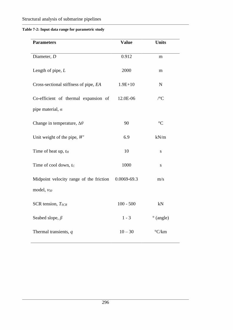
Structural analysis of submarine pipelines
296
Table 7-2: Input data range for parametric study
Parameters Value Units
Diameter, D 0.912 m
Length of pipe, L 2000 m
Cross-sectional stiffness of pipe, EA 1.9E+10 N
Co-efficient of thermal expansion of
pipe material, α
12.0E-06 /°C
Change in temperature, ∆θ 90 °C
Unit weight of the pipe, W′ 6.9 kN/m
Time of heat up, tH 10 s
Time of cool down, tC 1000 s
Midpoint velocity range of the friction
model, v50
0.0069-69.3 m/s
SCR tension, TSCR 100 - 500 kN
Seabed slope, β 1 - 3 ° (angle)
Thermal transients, q 10 – 30 °C/km

Structural analysis of submarine pipelines
297
Table 7-3: Non-dimensional parameters
Parameters Value
Characteristic velocity, ψ 0.000009-9.85
Characteristic strain, εc 0.00072

Structural analysis of submarine pipelines
298
Figures: F
rict
ion c
oef
fici
ent,
µ
Velovity, v (m/s)
µs
µk
µ = µk + (µs - µk )e-av
Increasing a
Figure 7-1: Sketch showing influence of a on friction factor
0
0.1
0.2
0.3
0.4
0.5
0.6
0.7
0.0001 0.001 0.01 0.1 1 10
Fri
ctio
n c
oef
fici
ent,
µ
Velovity, v (m/s)
v50
Drained, µUB
Undrained, µLB
µ = µLB + (µUB - µLB )e-λ(v/v50)
Figure 7-2: Nomenclature of velocity-dependent friction model

Structural analysis of submarine pipelines
299
0
0.2
0.4
0.6
0.8
1
1.2
0.0001 0.001 0.01 0.1 1
Resi
du
al s
tres
s ra
tio
, r
es/
s' n
o
Velocity (mm/s)
Soil P (SILT)
Marine clay (Hill
et al. 2012)
UWA kaolin
(White & Cathie 2011)
Storebælt till (Steenfelt 1993) OCR = 1 in
all cases
Figure 7-3: Published data showing effect of velocity on interface shear strength (White
et al. 2012)
0
0.2
0.4
0.6
0.8
1
1.2
0.0001 0.001 0.01 0.1 1
Res
idu
al s
tres
s ra
tio
, r
es/s
' no
Velocity (mm/s)
Soil P (SILT)
Marine clay (Hill
et al. 2012)
UWA kaolin
(White & Cathie 2011)
Storebælt till (Steenfelt 1993) Using decay
model
Figure 7-4: Fitting between data and friction rate model

Structural analysis of submarine pipelines
300
Velocity-dependent friction model between pipe and seabed
Figure 7-5: Benchmarking rate model with single element test on flat seabed
0.00001
0.0001
0.001
0.01
0.1
1
10
0 20 40 60 80 100 120
Vel
oci
ty,
v(m
/s)
Time, t (s)
Figure 7-6: Comparing velocities for single element test
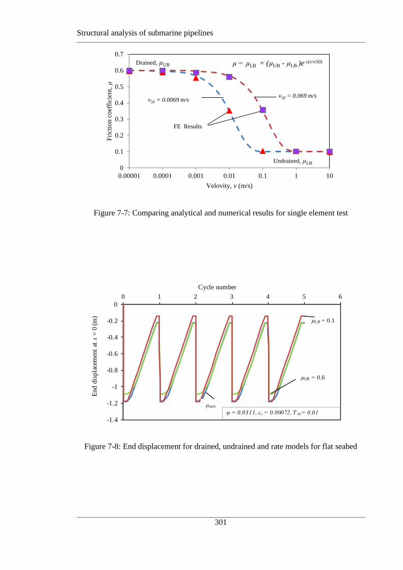
Structural analysis of submarine pipelines
301
0
0.1
0.2
0.3
0.4
0.5
0.6
0.7
0.00001 0.0001 0.001 0.01 0.1 1 10
Fri
ctio
n c
oef
fici
ent,
µ
Velovity, v (m/s)
v50 = 0.0069 m/sv50 = 0.069 m/s
Drained, µUB
Undrained, µLB
µ = µLB + (µUB - µLB )e-λ(v/v50)
FE Results
Figure 7-7: Comparing analytical and numerical results for single element test
-1.4
-1.2
-1
-0.8
-0.6
-0.4
-0.2
0
0 1 2 3 4 5 6
End
dis
pla
cem
ent
at x
= 0
(m
)
Cycle number
µUB = 0.6
µLB = 0.1
µrate
ψ = 0.0311, εc = 0.00072, T hc= 0.01
Figure 7-8: End displacement for drained, undrained and rate models for flat seabed
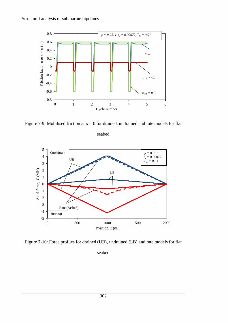
Structural analysis of submarine pipelines
302
-0.8
-0.6
-0.4
-0.2
0
0.2
0.4
0.6
0.8
0 1 2 3 4 5 6
Fri
ctio
n f
acto
r µ at x = 0 (
m)
Cycle number
µLB = 0.1
µUB = 0.6
µrate
ψ = 0.0311, εc = 0.00072, Thc = 0.01
Figure 7-9: Mobilised friction at x = 0 for drained, undrained and rate models for flat
seabed
-5
-4
-3
-2
-1
0
1
2
3
4
5
0 500 1000 1500 2000
Axia
l fo
rce,
P
(MN
)
Position, x (m)
UB
LB
Rate (dashed)
Cool down
Heat up
ψ = 0.0311
εc = 0.00072
Thc = 0.01
Figure 7-10: Force profiles for drained (UB), undrained (LB) and rate models for flat
seabed

Structural analysis of submarine pipelines
303
-0.8
-0.6
-0.4
-0.2
0
0.2
0.4
0.6
0.8
0 500 1000 1500 2000
Fri
ctio
n f
acto
r, (
dP
/dx)
/ W
'
Position, x (m)
UB (solid line)
LBRate (dashed)
ψ = 0.0311
εc = 0.00072
Thc = 0.01
Figure 7-11: Friction profiles for drained (UB), undrained (LB) and rate models for flat
seabed
-0.8
-0.6
-0.4
-0.2
0
0.2
0.4
0.6
0.8
700 800 900 1000 1100 1200 1300
Fri
ctio
n f
acto
r, (
dP
/dx)
/ W
'
Position, x (m)
UB (solid line)
LBRate (dashed)
Cool down
ψ = 0.0311
εc = 0.00072
Thc = 0.01
Figure 7-12: Enlarged view of central portion of friction profiles for flat seabed

Structural analysis of submarine pipelines
304
-5
-4
-3
-2
-1
0
1
2
3
4
5
0 200 400 600 800 1000 1200 1400 1600 1800 2000
Axia
l fo
rce,
P
(MN
)
Position, x (m)
Heat up
Cool down
TSCR = 500 kN
Rate (dashed)
UB(solid line)
LB
TSCR = 500 kN
εc = 0.00072
ψ = 0.0311
Thc = 0.01
Figure 7-13: Force profiles for drained (UB), undrained (LB) and rate models with TSCR
= 500 kN
-0.8
-0.6
-0.4
-0.2
0
0.2
0.4
0.6
0.8
0 500 1000 1500 2000
Fri
ctio
n f
acto
r, (
dP
/dx)
/W
'
Position, x (m)
Rate (dashed)
UB(solid line)
LB
TSCR = 500 kN
εc = 0.00072
ψ = 0.0311
Thc = 0.01
Figure 7-14: Friction profiles for drained (UB), undrained (LB) and rate models with
TSCR = 500 kN

Structural analysis of submarine pipelines
305
-5
-4
-3
-2
-1
0
0 1 2 3 4 5 6
End
dis
pla
cem
ent
at x
= 0
(m
)
Cycle number
µUB = 0.6
µLB = 0.1
µrate
TSCR = 500 kN
εc = 0.00072
ψ = 0.0311
Thc = 0.01
Figure 7-15: Walking responses for drained (UB), undrained (LB) and rate models with
TSCR = 500 kN
-5
-4
-3
-2
-1
0
1
2
3
4
5
0 500 1000 1500 2000
Axia
l fo
rce,
P
(M
N)
Position, x (m)
UB (solid
line)
LB
Rate (dashed)
Heat up
Cool down β = 3
ψ = 0.0311
εc = 0.00072
Thc = 0.01
β
Figure 7-16: Force profiles for drained (UB), undrained (LB) and rate models for
sloping seabed with β=3°
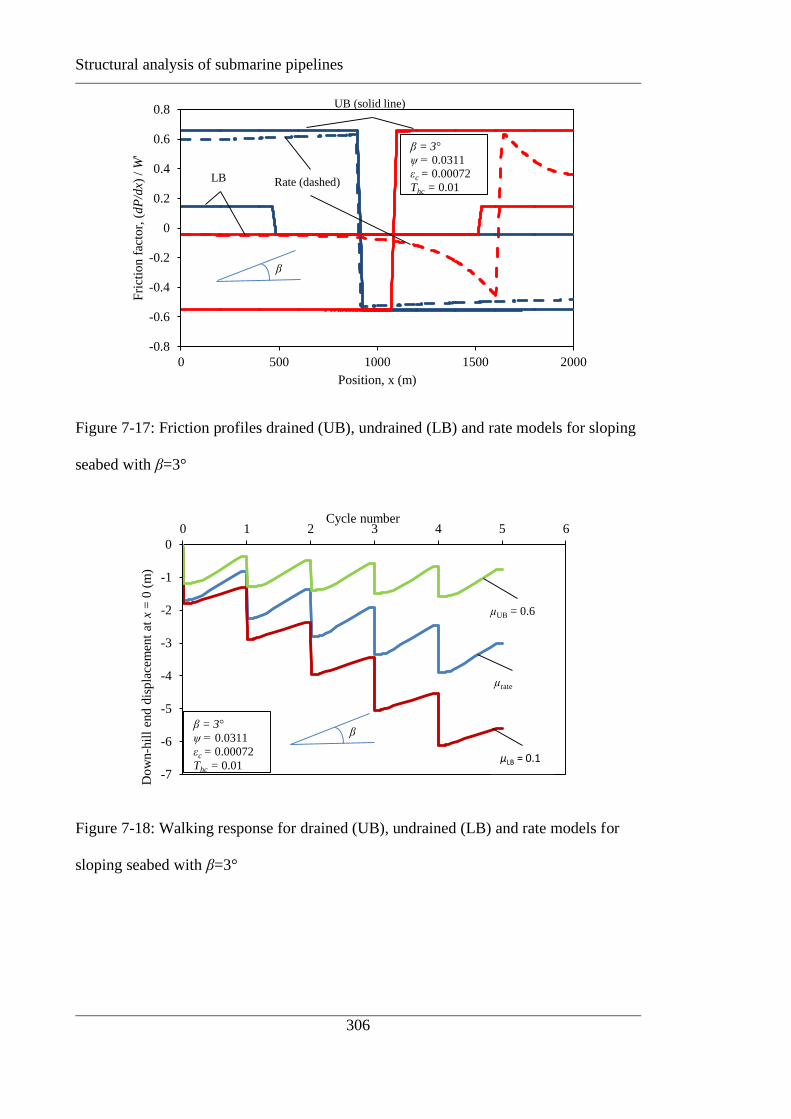
Structural analysis of submarine pipelines
306
-0.8
-0.6
-0.4
-0.2
0
0.2
0.4
0.6
0.8
0 500 1000 1500 2000
Fri
ctio
n f
acto
r, (
dP
/dx)
/ W
'
Position, x (m)
UB (solid line)
LB Rate (dashed)
β = 3
ψ = 0.0311
εc = 0.00072
Thc = 0.01
β
Figure 7-17: Friction profiles drained (UB), undrained (LB) and rate models for sloping
seabed with β=3°
-7
-6
-5
-4
-3
-2
-1
0
0 1 2 3 4 5 6
Do
wn-h
ill
end
dis
pla
cem
ent
at x
= 0
(m
)
Cycle number
µLB = 0.1
µUB = 0.6
µrate
β = 3
ψ = 0.0311
εc = 0.00072
Thc = 0.01
β
Figure 7-18: Walking response for drained (UB), undrained (LB) and rate models for
sloping seabed with β=3°

Structural analysis of submarine pipelines
307
0
0.2
0.4
0.6
0.8
1
1.2
0 1 2 3 4 5 6
Exp
ansi
on a
t co
ld e
nd
, u (
m)
Cycles
εc = 0.00072q = 10 °C/km
µUB = 0.6
µLB = 0.1 µdecay (dotted line)μrate (dashed)
Dis
pla
cem
ent at
cold
end, x
= 2
000 (
m)
Figure 7-19: Walking responses for drained (UB), undrained (LB) and rate models
for q = 10 °C/km
-5
-4
-3
-2
-1
0
1
2
3
4
5
0 500 1000 1500 2000
Axia
l lo
ad, P
(M
N)
Along the length, x (m)
εC = 0.00072q = 10 °C/km
ψ = 0.311
Cool down
Heat up
q = 10 C/km
εc = 0.00072
ψ = 0.0311
Thc = 0.01
Position, x (m)
Cycle 1
Cycle 2 - 5
Cycle 2 - 5
Rate model
Figure 7-20: Force profiles for, q = 10 °C/km

Structural analysis of submarine pipelines
308
-4
-3
-2
-1
0
1
2
-500 0 500 1000 1500 2000 2500
Axia
l d
isp
lace
men
t, u
(m)
Position, x (m)
P500 P1000 P1500
P2000
P0
TSCR = 500 kN
TSCR = 500 kN
εc = 0.00072
ψ = 0.0311
Thc = 0.01
Figure 7-21: Distributed displacements with rate model for SCR tension, TSCR = 500 kN
-4
-3
-2
-1
0
1
-500 0 500 1000 1500 2000 2500
Axia
l d
isp
lace
men
t, u
(m)
Position, x (m)
P0 P500 P1000 P1500P2000
β
β = 3
ψ = 0.0311
εc = 0.00072
Thc = 0.01
Figure 7-22: Distributed displacements with rate model for seabed slope, β = 3 °
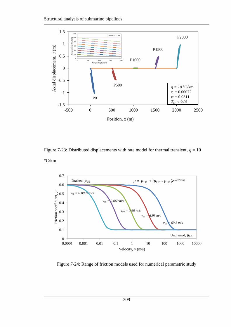
Structural analysis of submarine pipelines
309
-1.5
-1
-0.5
0
0.5
1
1.5
-500 0 500 1000 1500 2000 2500
Axia
l d
isp
lace
men
t, u
(m)
Along the length, x (m)
q = 10 °C/km
εC = 0.00072
ψ = 0.311
T = 0.01P0
P500
P1000
P1500
P2000
0
20
40
60
80
100
120
0 500 1000 1500 2000
Tem
pe
ratu
re p
rofi
le, θ
(°C
)
Along the length, x (m)
Gradient = 10°C/km
Position, x (m)
q = 10 C/km
εc = 0.00072
ψ = 0.0311
Thc = 0.01
Figure 7-23: Distributed displacements with rate model for thermal transient, q = 10
°C/km
Figure 7-24: Range of friction models used for numerical parametric study
0
0.1
0.2
0.3
0.4
0.5
0.6
0.7
0.0001 0.001 0.01 0.1 1 10 100 1000 10000
Fri
ctio
n co
effi
cien
t, µ
Velocity, v (m/s)
v50 = 0.0069 m/s
v50 = 0.069 m/s
v50 = 0.69 m/s
v50 = 6.93 m/s
Drained, µUB
Undrained, µLB
µ = µLB + (µUB - µLB )e-λ(v/v50)
v50 = 69.3 m/s
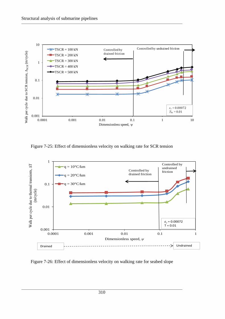
Structural analysis of submarine pipelines
310
0.001
0.01
0.1
1
10
0.0001 0.001 0.01 0.1 1 10
Wal
k p
er c
ycl
e d
ue
to S
CR
ten
sion
, ∆
SC
R(m
/cy
cle)
Dimensionless speed, ψ
TSCR = 100 kN
TSCR = 200 kN
TSCR = 300 kN
TSCR = 400 kN
TSCR = 500 kN
Controlled by
drained friction
Controlled by undrained friction
εc = 0.00072
Thc = 0.01
Figure 7-25: Effect of dimensionless velocity on walking rate for SCR tension
Figure 7-26: Effect of dimensionless velocity on walking rate for seabed slope
0.001
0.01
0.1
1
0.0001 0.001 0.01 0.1 1
Wal
k pe
r cy
cle
due
to t
herm
al t
rans
ient
s, ∆
T
(m/c
ycle
)
Dimensionless speed, ψ
q = 10°C/km
q = 20°C/km
q = 30°C/km
Drained Undrained
εc = 0.00072T = 0.01
Controlled by
drained friction
Controlled by
undrained
friction
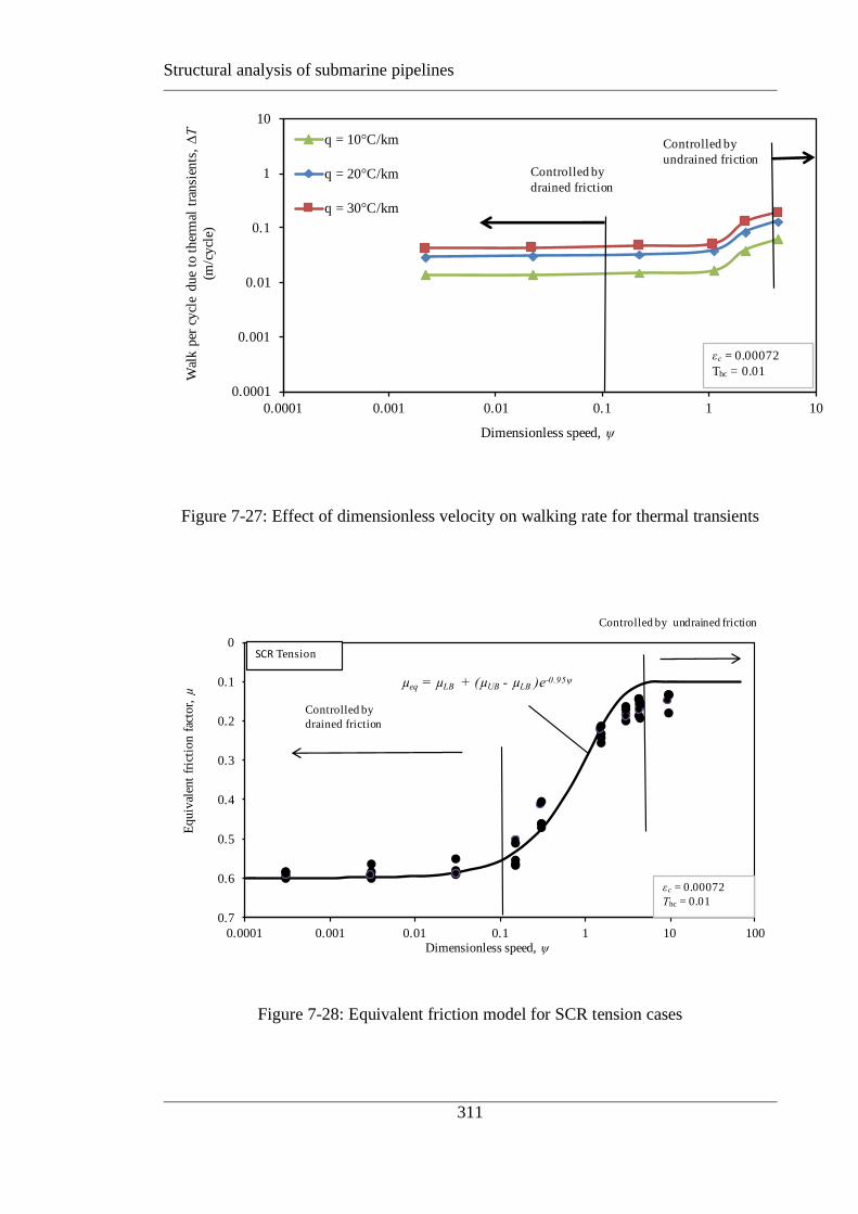
Structural analysis of submarine pipelines
311
0.0001
0.001
0.01
0.1
1
10
0.0001 0.001 0.01 0.1 1 10
Wal
k p
er c
ycl
e du
e to
ther
mal
tra
nsi
ents
, ∆
T
(m/c
ycl
e)
Dimensionless speed, ψ
q = 10°C/km
q = 20°C/km
q = 30°C/km
εc = 0.00072
Thc = 0.01
Controlled by
drained friction
Controlled by
undrained friction
Figure 7-27: Effect of dimensionless velocity on walking rate for thermal transients
0
0.1
0.2
0.3
0.4
0.5
0.6
0.7
0.0001 0.001 0.01 0.1 1 10 100
Eq
uiv
alen
t fr
icti
on
fac
tor,
µ
Dimensionless speed, ψ
εc = 0.00072
Thc = 0.01
SCRTension
Controlled by
drained friction
µeq = µLB + (µUB - µLB )e-0.95ψ
Controlled by undrained friction
Figure 7-28: Equivalent friction model for SCR tension cases

Structural analysis of submarine pipelines
312
0
0.1
0.2
0.3
0.4
0.5
0.6
0.7
0.0001 0.001 0.01 0.1 1 10 100
Eq
uiv
alen
t fr
icti
on f
acto
r, µ
Dimensionless speed, ψ
Controlled by
drained friction
Controlled by undrained friction
Seabed slope
µeq = µLB + (µUB - µLB )e-0.95ψ
εc = 0.00072
Thc = 0.01
Figure 7-29: Equivalent friction model for sloping seabed cases
0
0.1
0.2
0.3
0.4
0.5
0.6
0.7
0 0.1 0.2 0.3 0.4 0.5 0.6 0.7
Cal
cula
ted
fri
ctio
n f
acto
r, μ
_ca
lcu
late
d
Proposed equivalent friction factor, μ_proposed
T_hc= 0.001
T_hc = 0.01
T_hc = 0.1
T_hc = 1
T_hc= 10
T_hc= 100
T_hc= 1000
εc = 0.00072β = 3°tc = 1000 s
µeq = µLB + (µUB - µLB )e-0.95ψ
Figure 7-30: Comparison between proposed and calculated friction factors for varying Thc
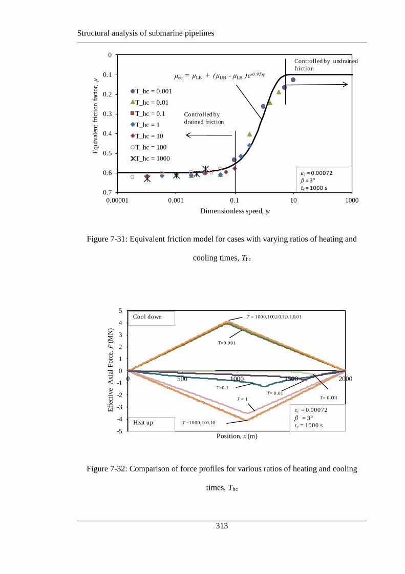
Structural analysis of submarine pipelines
313
0
0.1
0.2
0.3
0.4
0.5
0.6
0.7
0.00001 0.001 0.1 10 1000
Eq
uiv
alen
t fr
icti
on f
acto
r, µ
Dimensionless speed, ψ
T_hc = 0.001
T_hc = 0.01
T_hc = 0.1
T_hc = 1
T_hc = 10
T_hc = 100
T_hc = 1000
εc =0.00072β =3°tc =1000s
µeq = µLB + (µUB - µLB )e-0.95ψ
Controlled by undrained
friction
Controlled by
drained friction
Figure 7-31: Equivalent friction model for cases with varying ratios of heating and
cooling times, Thc
-5
-4
-3
-2
-1
0
1
2
3
4
5
0 500 1000 1500 2000
Eff
ecti
ve
Axia
l F
orc
e,P
(M
N)
Position, x (m)
Cool down
Heat up
T = 1000,100,10,1,0.1,0.01
T =1000,100,10
T = 1
T=0.1
T= 0.01
εc = 0.00072
β = 3°
tc = 1000 s
T=0.001
T= 0.001
Figure 7-32: Comparison of force profiles for various ratios of heating and cooling
times, Thc

Structural analysis of submarine pipelines
314
0
0.1
0.2
0.3
0 0.0004 0.0008 0.0012 0.0016
Wal
k p
er c
ycl
e d
ue
to s
eab
ed s
lop
e, ∆
Φ
(m/c
ycl
e)
Characteristic strain, εc
ψ = 0.0311
Thc= 0.01
β = 3
β = 1
Figure 7-33: Effect of characteristic strain on walking rate of pipe for various weights
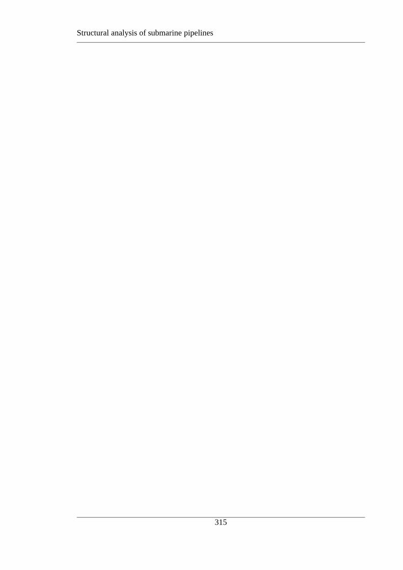
Structural analysis of submarine pipelines
315

Structural analysis of submarine pipelines
316
Structural analysis of submarine pipelines
317
CONCLUSIONS AND FUTURE WORK
OVERVIEW
The proposed research was concerned with the structural behaviour of submarine
pipeline subjected by submarine slides, and thermal loading conditions. The research aim
was to support the transition of oil and gas developments into deeper water and more
remote conditions. This was achieved by improving the techniques for assessing the axial
pipe-soil interaction forces resulting from relative pipe-soil movement, including the
passage of mobile slide material along or across a seabed pipeline.
CONCLUDING REMARKS
In this chapter the main findings, concluding remarks along with possible directions
for future work are presented. Throughout the thesis analytical models were developed to
tackle the pipe-soil interaction issues and structural problems and numerical solutions
were provided. Where appropriate, the theoretical techniques used for pile design were
transferred to pipeline conditions.
8.1.1 Elastic stiffness
Limited information exists in the literature on the axial elastic pipe-soil response of
on-bottom pipelines, particularly for nonhomogeneous soil. Therefore, an approximate
analytical approach was developed for axial stiffness, focusing on the case of shear
modulus proportional to depth. The solution was then verified through numerical analysis.
Further numerical analysis was carried out to obtain relationships for horizontal and

Structural analysis of submarine pipelines
318
vertical elastic stiffnesses of on-bottom pipelines. Here the author provided
recommendation for the selection of proper elastic stiffnesses in all three directions of
motion. These recommendations allow consistent and rigorous modelling of elastic pipe–
seabed interactions with application to the analysis of pipeline laying, buckling, walking,
and on-bottom stability. They have found adoption in practice and have recently been
referenced in the new DNV code for pipe-soil interaction (DNVGL-RP-F114, 2019).
The contributions in chapter 3 lay the basic foundation for the following chapters on axial
slide-pipeline interaction and then buckling analyses due to axial loading. Once the axial
elastic stiffness is known, then the ultimate axial resistance was evaluated and axial
springs were formulated and implemented into the FE code to carry out the structural
analyses of pipeline.
8.1.2 Submarine slide pipeline interactions
In Chapter 4 an analytical solution was developed for axial submarine slide loading
of a straight on-bottom pipeline. It was shown that the non-dimensional axial loads and
axial displacements depend on three non-dimensional input parameters, i.e. the driving
force in the slide zone, seabed resisting force in passive zone, and pipe-soil stiffness. Non-
dimensional design charts were presented to show the effect of individual input
parameters on axial loads and axial displacements. The maximum axial load in the pipe
is directly proportional to the slide force, while the load at the transition from elastic to
plastic soil resistance is initially proportional to the slide force but then becomes limited.
The limit is reached for most relevant values of the slide force. Numerical FE analysis
was also carried out to verify the analytical model. Analytical and numerical solutions
were shown to match with close agreement. The buckling was ignored in the analytical
model. However, the existing classical theory of buckling was linked to the output of the

Structural analysis of submarine pipelines
319
analytical model to show the vulnerability of the pipelines towards buckling in case of
various slide loading conditions. On bottom submarine pipelines are more susceptible to
lateral buckling when impacted axially by stronger and longer slides.
8.1.3 Lateral buckling of submarine pipelines
Lateral buckling analysis of on-bottom submarine pipelines is of particular interest
in the offshore industry due to the complexities involved in the analysis, and the potential
design efficiencies that can be unlocked. Classical buckling theories by previous
researchers and recent joint industry projects provide a basis for estimation of the critical
buckling load of a straight, or in some cases imperfect, pipe on either a rigid or elastic
seabed. However, systematic solutions for the combined effects of nonlinear soil
properties and the as-laid geometry – specifically the out-of-straightness – on the buckle
initiation behaviour have not been developed previously.
In Chapter 5, an investigation of the buckling problem of an imperfect (non-
straight) on-bottom pipeline subjected to axial compressive loading was carried out. The
seabed was modelled with lateral and axial elastic, perfectly plastic, springs to idealise
the load-displacement behaviour of the soil and the pipe was modelled with pipe elements.
Buckling was performed by a displacement controlled finite element method with the
modified RIKS algorithm that is available in the commercial software ABAQUS. This
numerical tool was used to develop a parametric solution for the present problem in terms
of the various pipe material and geometry parameters and the lateral and axial pipe-soil
interaction parameters. In particular, the influence of the magnitude and stiffness of the
lateral pipe-soil response was investigated, highlighting the sensitivity of the pipeline
response to the geotechnical inputs. The results have been synthesised in a generic non-
dimensionalised design chart to estimate the buckling load, valid for the range of inputs
covered by the parametric study.
Structural analysis of submarine pipelines
320
The chapter presented a new solution for the buckling force that includes both
OOS and initial stress. It was found that for the range of parameters investigated the effect
of the axial stress can be introduced simply as a new dimensionless group, without
changing the influence of the other groups in the correlation. This contribution provides
a more efficient basis for predicting buckling behaviour, and highlights in a simple way
the relative influence of the controlling parameters.
8.1.4 Submarine Pipeline Walking
In analytical modelling the pipe-soil interaction is usually modelled as rigid-
plastic, expressed as ultimate resistance per unit length. Often this term is expressed non-
dimensionally as a friction factor, µ, which is the ratio of axial resistance, F, to submerged
pipe weight, W. However, the elastic-plastic (i.e. bi-linear) behaviour of the soil and the
effect of this bi-linear response of the soil on the walking behaviour were poorly
addressed in the existing body of knowledge. The elastic-plastic behaviour is often
represented by an additional parameter, specified as the mobilisation displacement. This
is defined as the amount of axial displacement that occurs before the ultimate friction is
generated, and the resistance rises linearly with displacement up to this value. The
walking behaviour is affected by the axial friction mobilisation displacement. Numerical
results were observed by previous researchers. However, the analytical solution for the
reduction of walking per cycle due to increase in mobilisation displacement has not been
attempted elsewhere. In Chapter 6, a numerical study was reported, which provides
insight into the walking behaviour due to seabed slope, SCR tension and thermal
transients. The existing analytical solutions were extended to incorporate the elastic-
plastic response of the soil into the expression of pipeline walking and a new derivation
was proposed. Numerical verification with ABAQUS was also done for the proposed

Structural analysis of submarine pipelines
321
expression. The resulting expression and calculation method extends existing analytical
solutions for walking to a wider range of conditions.
In conventional analyses, seabed friction is independent of the rate of thermal
loading and expansion but it has been recognised that the sliding resistance between a
pipe and the seabed varies with velocity, partly due to drainage effects. In Chapter 7 the
numerical model that was validated in the previous chapter is extended to explore the
effect of velocity-dependent seabed friction. A velocity-dependent friction model is
implemented in commercial software ABAQUS and validated via single element and
simple (flat seabed) pipeline cases. This model features upper and lower friction limits,
with a transition that occurs as an exponential function of velocity. A parametric study
was performed using differing rates of heating and cool-down in walking situations driven
by seabed slope, SCR end tension and the difference between heat up and cool down rates.
The walking behaviour is compared to cases with constant friction and solutions are
proposed to express the velocity-dependent response in terms of an equivalent constant
friction. These equivalent friction values can then be applied in existing simple solutions
or more complex numerical analyses, as a short cut method to account for velocity-
dependent friction.
FUTURE RESEARCH
The new developments of oil and gas infrastructure are moving into deeper water.
This requires design and construction of long high temperature and high pressure
pipelines from deep sea to shore. These pipelines are subjected to cyclic expansion during
operating cycles and geohazards such as submarine slides. Concluding remarks out of this
research have been detailed in the above section and some of the future research scopes
are highlighted in the section below, as follows:
Structural analysis of submarine pipelines
322
1. The research in this thesis has been exclusively theoretical, building on existing
theory and published data on submarine pipeline soil interaction in order to
substantiate the proposed models of submarine pipeline behaviour under the slide and
thermal loading. The analytical models were limited to elastic limits of the pipe
material and the finite element analyses were confined and limited due to the SSFE
methods for elastic stiffness prediction. These solutions can be extended to multiple
directions of loading, in order to identify the coupling between the elastic and plastic
responses in each direction. This would be an improvement over current practice,
where independent springs are ‘attached’ to the pipe for each direction of motion.
This coupling is already recognised and quantified for vertical-lateral (V-H) loading
(e.g. Randolph & White 2008). To illustrate this potential future work, the FE model
developed in chapter 3 has been used to generate a V-H yield envelope for typical soil
parameters. A fully bonded pipe-soil interface was considered and V-H swipes were
performed to establish the yield envelope in vertical-horizontal space. Homogeneous
soil with uniform shear strength of (su = 5 kPa) was considered. The resulting V-H
envelopes matched the existing literature for all the embedment cases. The same
methodology was used to provide the V-F and H-F yield envelopes for exactly similar
cases, to identify potential vertical-axial or lateral-axial coupling. As shown in the
Figure 8-1and Figure 8-2, there is coupling, meaning that when a significant fraction
of either the vertical or lateral capacity is mobilised, the available axial resistance is
reduced. This may influence the response of pipeline in buckles and submarine slides,
where both the axial and lateral resistance is concurrently mobilised. For future work,
these SSFE example could be extended to large deformation FE (LDFE) analysis with
more complex soil and pipe-soil interface behaviour.
Structural analysis of submarine pipelines
323
2. In the analytical axial slide pipeline interaction problem - the slide loading was
considered to be a constant distributed load and the pipe was considered to be
perfectly straight and elastic in nature. However, the complexities associated with the
as-laid geometry of the pipe along with its elastic-plastic material behaviour need to
be studied in the future research. At the same time studies need to be extended for
dynamic loading conditions where the shear strength of the slide material changes
along its travel path to check the structural integrity of the pipelines along its length
under that condition.
3. For the lateral buckling on submarine pipeline the numerical model developed in this
thesis needs to be extended with dynamic simulation and with nonlinear user defined
elements representing a detailed pipe-soil interactions to validate the parametric
solution. Furthermore the methodology can be used to provide solution in the vertical
direction, and where there is out-of-straightness present from the lay process prior to
the thermal loading.
4. All the structural analyses in this thesis involve a rigid or elastic seabed. During lateral
buckling, the pipe may undergo large lateral displacement and bending strains,
including movement in the vertical plane. Therefore, simultaneous modelling of
structural and geotechnical responses using a full three-dimensional (3D) model may
be a pragmatic solution. However, full 3D modelling of large deformation effects of
both structural and soil domains is a significant challenge from a project schedule and
numerical (FE) perspective. With the advent of supercomputers, and also new solver
techniques, full 3D modelling of simultaneous structural and geotechnical responses
could add value in the body of knowledge in the near future.
5. For pipeline walking – the analytical solution with bi-linear soil-pipe interaction, and
the numerical solution with velocity dependent friction model need to be verified with
Structural analysis of submarine pipelines
324
the field data from various joint industry projects and also with the experimental data
through full scale laboratory test to predict walking behaviour more accurately for
different soil conditions. Thereafter, comprehensive parametric analysis need to be
carried out to provide more generic design charts for the pipeline engineers as a guide.
Regardless of limitations of the current work and scope for future research, it is
considered that the outcomes of this research present several useful contributions to the
current body of knowledge of pipe-soil interaction and structural analysis. They also
provide validation and standardisation of existing calculation methods for structural
analysis of submarine pipeline and pipe-soil interaction, and have produced new analysis
techniques that can be utilised to investigate project-specific refinements.

Structural analysis of submarine pipelines
325
References:
DNVGL-RP-F114, DNV Recommended Practice F114. Pipe-soil interaction for
submarine pipelines. (2019). Det Norske Veritas, Norway Sept 2019.
Randolph M.F. & White D.J. 2008. Upper bound yield envelopes for pipelines at shallow
embedment in clay Géotechnique, 58(4):297-301

Structural analysis of submarine pipelines
326
Figures
Figure 8-1: Failure envelop in the vertical - axial space
Figure 8-2: Failure envelop in the horizontal/lateral - axial space
0
0.2
0.4
0.6
0.8
1
1.2
1.4
1.6
1.8
0 1 2 3 4 5 6 7
No
rmal
ised
ax
ial
resi
stan
ce,
F/s
uD
Normalised vertical resistance, V/suD
w/D = 0.1 to 0.5
0
0.2
0.4
0.6
0.8
1
1.2
1.4
1.6
1.8
0 0.5 1 1.5 2 2.5 3 3.5 4
Norm
alis
ed a
xia
l re
sist
ance
, F
/suD
Normalised lateral resistance, H/suD
w/D = 0.1 to 0.5

Structural analysis of submarine pipelines
327

Structural analysis of submarine pipelines
328