Hafez et al. Beni-Suef Univ J Basic Appl Sci (2022) 11:36 https://doi.org/10.1186/s43088-022-00219-x

RESEARCH

Dynamic on-bottom stability analysis of subsea pipelines using finite element model-based general offshore analysis software: a case studyKhaled A. Hafez1, Mohammed A. Abdelsalam1* and Ahmed N. Abdelhameed2,3

Abstract

Background: The dynamic on-bottom stability analysis represents a fundamental task in the design process of the subsea pipelines. Such analysis ensures the stability of the as-laid pipeline on the seabed against the lateral displace-ments, which are induced by the surrounding hydrodynamic forces. In this paper, the dynamic on-bottom stability analysis of a subsea pipeline is performed using finite element-based advanced offshore engineering simulation software called Flexcom. The latter predicts the pipeline response in a time-domain simulation based on a given envi-ronmental condition (i.e., the sea state, the soil frictional resistance, and the nonlinear behavior of the pipeline). A case study is conducted on a 22-in.-diameter pipeline, which is placed on a sandy soil in shallow water, under different loading combinations from two-dimensional irregular waves and a steady current.

Results: The resultant maximum lateral displacements and the associated stresses decreased by increasing the con-crete weight coating thickness. Pipeline response due to drag, lift, and inertia forces increased by increasing the total water particle velocity induced from the summation of wave-induced particle velocity and current velocity. Different random wave patterns generated from different random seed numbers assigned to wave components are important to verify the selection of the concrete weight coating thickness. Ignoring passive soil resistance reduced the total soil resistance significantly and resulted in conservative stability weight requirement.

Conclusions: Several factors influence the pipeline stability such as pipeline submerged weight, hydrodynamic loads induced by random sea states, and soil friction model being used. The dynamic on-bottom stability analysis can optimize the design and results in less concrete weight coating if the actual case is modeled accurately; therefore, ignoring passive soil resistance reduced the prime advantage of this analysis compared to other simplified methods.

Keywords: Dynamic on-bottom stability, Pipe–soil interaction, Subsea pipelines, Finite element analysis (FEA), Hydrodynamic loads, Time-domain simulation

© The Author(s) 2022. Open Access This article is licensed under a Creative Commons Attribution 4.0 International License, which permits use, sharing, adaptation, distribution and reproduction in any medium or format, as long as you give appropriate credit to the original author(s) and the source, provide a link to the Creative Commons licence, and indicate if changes were made. The images or other third party material in this article are included in the article’s Creative Commons licence, unless indicated otherwise in a credit line to the material. If material is not included in the article’s Creative Commons licence and your intended use is not permitted by statutory regulation or exceeds the permitted use, you will need to obtain permission directly from the copyright holder. To view a copy of this licence, visit http:// creat iveco mmons. org/ licen ses/ by/4. 0/.

1 BackgroundVarious design methods may be employed for on-bottom stability assessment of the subsea pipelines on the basis of hydrodynamic loads and soil resistance. These meth-ods may be split into three categories as follows [49]. The first category includes the static analysis methods which are based on the force-balance calculation that is firstly introduced in DNV 1976 [15] and in which the

Open Access

Beni-Suef University Journal ofBasic and Applied Sciences

*Correspondence: eng-mohammed.abdelsalam@alexu.edu.eg1 Department of Naval Architecture and Marine Engineering, Faculty of Engineering, Alexandria University, Post Code 21544, El-Chatbi, Alexandria, EgyptFull list of author information is available at the end of the article

Page 2 of 17Hafez et al. Beni-Suef Univ J Basic Appl Sci (2022) 11:36

pipeline movement is not allowed under the extreme sea state; these methods include Level 1 program of Pipeline Research Council International (PRCI) of the American Gas Association (AGA) and absolute lateral static stabil-ity (ALSS) method presented in RP-F109 [16]. The sec-ond category includes the empirical or calibrated design methods such as the Level 2 program of the PRCI of the AGA [18, 33] which is known as AGA Level 2, and the generalized lateral stability (GLS) method presented in RP-F109 [16, 17, 25]. The third category includes the dynamic lateral stability (DLS) analysis, which is based on the time-domain simulation of the pipeline dynamic response, the sea state-induced hydrodynamic loads, and the pipe–soil interaction, using specialized finite element (FE) software packages. The DLS analysis usually repre-sents the basis for validating other calibrated methods, to ensure stability and to provide lower-conservative and higher-optimized design.

The DLS analysis method is not widely used because of the associated complexities than other conventional sta-bility methods that are represented by building a model with accurate simulation involving the fluid–pipe–soil interaction, the limited availability of the software pack-ages, and the incentive to replace the static and calibrated methods with advanced dynamic ones is not existing [41]. In this regard, there are only two software packages recognized in the industry for the dynamic on-bottom stability analysis of the subsea pipelines: PONDUS [21] and AGA Level 3 [1, 26, 33]. It is possible to use the other general FE software packages such as ABAQUS [12] and ANSYS [4] with integrated modules for modeling the hydrodynamic loads and the pipe–soil interaction. Ose et  al. [31] introduced the first finite element model using ABAQUS [20] for the dynamic on-bottom stability analysis of the pipelines by using simplified modeling of the hydrodynamic loads and the mutual pipe–soil inter-action. Bai and Yu [8] used ABAQUS to compare the on-bottom stability analysis results from the finite ele-ment model versus  RP-E305 [13] to ensure the validity of the numerical model. ABAQUS has also been used to build and solve the numerical model of pipeline stability problems using a finite element method as presented in Yang and Wang [47] and Bai et  al. [7]. Based on differ-ent methodologies of calculating the hydrodynamic loads and the pipe–soil interaction, other modules have been developed and integrated with the ABAQUS FE solver for dynamic on-bottom stability analysis of the pipelines. These modules are referred to by different names, such as SIMSTAB [50], UWAINT [40], and CORUS-3D [6]. SIMSTAB has been utilized in several case studies as pre-sented in Ref. [3, 24, 34]. UWAINT has been developed based on several numerical models developed by  Tian and Cassidy [37–39]. CORUS-3D has been used to study

the dynamic response of pipelines as presented in  Ref. [23, 28, 48].

Offshore software packages such as Flexcom [46] and OrcaFlex [30] may also be used as will be described in the subsequent sections of this paper by using Flexcom soft-ware [46].

In this paper, the DLS analysis is conducted on a 22-in.-diameter pipeline installed in shallow water on a sandy seabed. The sea state consists of irregular waves, represented by the Joint North Sea Wave Project (JON-SWAP) spectrum [19], and a steady current. It is worth mentioning that this paper is devoted to studying the installation phase of the pipeline with an empty condi-tion, as a worst case, under the following combined loads from waves and currents: 1-year return period  values (RPV) wave + 10-year RPV current and 10-year RPV wave + 1-year RPV current.

The acceptance criteria of the on-bottom stability design of the pipelines depend on the design target and the factors that may affect the integrity of the pipeline. The acceptance criteria may be achieved either by the maximum allowable lateral displacement of the pipe-line or by the stress limits for the design of the pipeline. Using both criteria, the numerical results are presented (sequentially) in the relevant subsections of this paper.

2 MethodsThe dynamic on-bottom stability analysis of a subsea pipeline is performed by using finite element-based advanced simulation software, which is named Flex-com [46]. Flexcom is a highly versatile software package, which is commonly used in the structural analysis of con-ventional and unconventional offshore structures. The pipeline is modeled as a line with an automatic mesh gen-eration, depending on the specified element length. The structural geometric properties (i.e., internal and external diameters, wall thickness, Young’s modulus, shear modu-lus, mass density, etc.) are assigned to the pipeline. The hydrodynamic loads in the form of drag, inertia, and lift force coefficients are allocated to the pipeline. The exter-nal and internal coatings, such as corrosion and concrete coatings, are added by deciding the thickness of each coating layer. The sea state consists of two-dimensional irregular waves accompanied by a steady current, and both are perpendicular to the pipeline.

Figure 1 shows the external forces (including the water-induced hydrodynamic forces, the self-weight of the pipeline, and the soil resistance) which affect the subsea pipeline segment.

The time-domain simulation is performed for a dura-tion of 3 h (10,800 s), as recommended in RP-F109 [16]. To perform full dynamic stability analysis for the pipe-line, three different types of analyses are performed and

Page 3 of 17Hafez et al. Beni-Suef Univ J Basic Appl Sci (2022) 11:36

then subsequently aggregated into one dynamic analy-sis. These three types of analyses include static analysis, quasi-static analysis, and time-domain dynamic analysis.

The static analysis is performed to study the effect of the time-independent loadings such as water current and temperature loadings. In such analysis, the full model is designed to include the geometrical layout of the pipe-line and its material and hydrodynamic properties, the environmental properties, as well as the geomechanical properties of the soil (shear strength, friction, adhesion, compressibility, abrasion, corrosion, permeability, seep-age, lateral earth pressure, consolidation, bearing capac-ity, slope stability), and geotechnical properties of the soil (grain-size distribution, weight–volume relationships, relative density, Atterberg/consistency limits, soil texture, soil phases, etc.).

In the quasi-static analysis, all vertical constraints along the length of the pipeline are removed, and the pipeline is allowed to fall onto the seabed, under the combined effect of the gravity and buoyancy loads. Settling the pipeline quickly over the seabed under the combined effect of the gravity and buoyancy loads may be per-formed by specifying a significant mass damping to mini-mize initial transients. It is worth mentioning that the static and quasi-static analyses merely facilitate contact initiation between the pipeline and the seabed for pen-etration, due to the mutual action of pipeline self-weight and the seabed soil stiffness.

The dynamic analysis is performed in the time domain, to investigate the effect of the time-dependent loads (e.g., the wave loads, etc.), and the nonlinear response of the concrete-coated pipeline. For a given design condition,

in which the pipeline is required to withstand combined static and dynamic loads, Flexcom [46] builds a fully dynamic solution for the combined loads by superpos-ing the static, quasi-static, and dynamic analyses and then integrating all loads through all stages to get the full response of the pipeline at the end of the dynamic simulation.

2.1 Pipe–soil interactionThe interaction between the concrete-coated pipeline and the soil plays a significant role in the overall pipe-line response and its contribution to the on-bottom stability as a resisting force to the surrounding hydro-dynamic loads. Pipe–soil interaction is a very complex process because of the mutual influence between several parameters occurring throughout the pipeline installa-tion and operation conditions. These parameters include the hydrodynamic cyclic loading on the pipeline and the pipe–soil interaction. Different hydrodynamic mod-els have been developed based on the Morison’s equa-tions [29] to accurately predict the cyclic loadings on the pipeline from waves and currents. These models were developed in Ref. [11, 17, 22, 25, 35, 36, 42].

The seabed soil resistance consists mainly of two com-ponents: the friction between the pipeline and the seabed soil (i.e., pure friction term) and the resistance due to the embedment of the pipeline into the seabed soil (i.e., passive resistance term). Lyons [27] experimentally con-cluded that the Coulomb friction model was not appro-priate to describe the pipe–soil interaction, especially when the pipeline is placed on a soil of soft clay or loose

Weight

Fig. 1 Forces affecting subsea pipeline

Page 4 of 17Hafez et al. Beni-Suef Univ J Basic Appl Sci (2022) 11:36

sand. Coulomb friction model does not function in the properties of wave, pipe, and soil.

The passive soil resistance models have initially been developed through the PIPESTAB project [10, 45] and then the AGA project [1, 9]. Both models were appropri-ate for use in predicting the dynamic pipeline response and for soft clay and loose sand soils, and both are imple-mented in PONDUS [21] and AGA software [33], respec-tively. By revisiting the PIPESTAB [10, 45] and AGA [1, 9] test data and other test data sources [32], an empiri-cal approach was proposed by  Verley and Sotberg [44] and Verley and Lund [43] to evaluate embedment for sand and clay soils, respectively. Both empirical approaches are considered the basis for the current design method-ologies represented in RP-F109 [16].

Neglecting the passive soil resistance results in decreas-ing its total soil resistance (compared to its actual resist-ance); especially when the pipeline is placed on soil of soft clay or loose sand, the m utual interaction between the pipeline and the seabed soil may not be modeled accurately [49], and the pipeline may also large ly displace in the lat eral direction.

In the present case study, only the pure friction term is considered, due to the present capabilities of the soft-ware, and it is represented herein by the Coulomb fric-tion model. The Coulomb friction model is considered as the simplest method for modeling the interaction between the pipeline and the seabed soil, and it can be used in both the static and dynamic analysis [49]. The Coulomb friction model assumes pure steady plastic frict ional resistance between the pipeline and the seabed soil, and it does not consider any embedment-based cyclic loads or passive soil resistance.

To ensure the stability of the pipeline on the seabed in the presence of the Coulomb friction model, Eq. (1) must be satisfied.

where Ff is the friction force induced by the wave and current between the pipeline and the seabed in a direc-tion parallel to the seabed, µ is the coefficient of friction between the pipeline and the seabed, and Fc is the con-tact force induced by the wave and current between the pipeline and the seabed in a direction perpendicular to the seabed: Fc = Ws − FL , in which Ws is the pipeline submerged weight in a direction perpendicular to its span and FL is the lift force induced by the wave and cur-rent in a direction perpendicular to the pipeline.

The seabed is modeled as an elastic flat surface hav-ing longitudinal and transverse friction coefficients and a constant linear stiffness value. For the concrete-coated pipelines (as per the present case study), the RP-F109

(1)Ff ≤ µFc

[16] recommends a friction coefficient ( µ ) of 0.6 for sand and rock soil and 0.2 for clay soil.

At each iteration step of the time-domain simula-tion, the software surveys all the nodes of the structural model of the pipeline, to check whether they are in con-tact with the seabed or not (as long as either a rigid or elastic seabed has been specified as part of the model). If any node registered such contact, and if either or both of the seabed friction coefficients are nonzero, it is assumed as attached to the seabed (in the plane of the seabed) using a friction coefficient-based nonlinear spring approach.

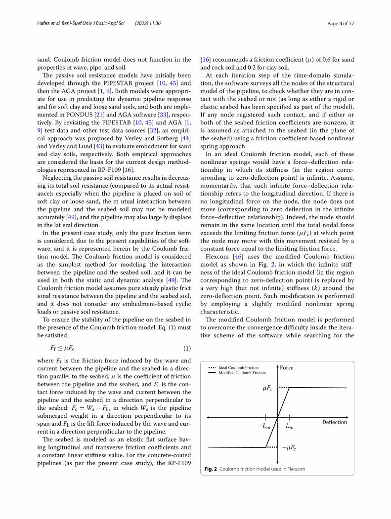
In an ideal Coulomb friction model, each of these nonlinear springs would have a force–deflection rela-tionship in which its stiffness (in the region corre-sponding to zero-deflection point) is infinite. Assume, momentarily, that such infinite force–deflection rela-tionship refers to the longitudinal direction. If there is no longitudinal force on the node, the node does not move (corresponding to zero deflection in the infinite force–deflection relationship). Indeed, the node should remain in the same location until the total nodal force exceeds the limiting friction force ( µFc ) at which point the node may move with this movement resisted by a constant force equal to the limiting friction force.

Flexcom [46] uses the modified Coulomb friction model as shown in Fig.  2, in which the infinite stiff-ness of the ideal Coulomb friction model (in the region corresponding to zero-deflection point) is replaced by a very high (but not infinite) stiffness ( k ) around the zero-deflection point. Such modification is performed by employing a slightly modified nonlinear spring characteristic.

The modified Coulomb friction model is performed to overcome the convergence difficulty inside the itera-tive scheme of the software while searching for the

Ideal Coulomb FrictionModified Coulomb Friction

Fig. 2 Coulomb friction model used in Flexcom

Page 5 of 17Hafez et al. Beni-Suef Univ J Basic Appl Sci (2022) 11:36

correct solution of the deflections (as in the case of most FE programs). This point is crucial to the opera-tion of the seabed friction model. As the displacement at any arbitrary node depends, principally, on the stiff-ness of this section of the force–deflection curve, the stiffness is given by Eq. (2).

where k is the stiffness of the Coulomb friction model and Lm is the mobilization length which is taken as 5% of steel pipeline outer diameter.

The value of the mobilization length ( Lm ) affects the stiffness of the nonlinear spring, i.e., the smaller is this value, the greater is the stiffness and the closer the fric-tion model is to an ideal model. However, reducing the mobilization length of the pipeline makes it harder for the program t o converge on a correct solution of the deflections. Note also that separate mobilization lengths may be used in both the longitudinal and transverse directions, with the longitudinal value typically being shorter than the transverse one.

2.2 Environmental loadsThe environmental loads on the subsea pipelines, for an arbitrary-selected sea state, are represented by a combi-nation of two-dimensional irregular waves and current loadings. Such loads are assumed to be dependent on the total velocity of water particles at the pipeline level and pipeline velocity. The total velocity of water parti-cles is calculated as the summation of the wave-induced particle velocity and the steady current velocity. The wave-induced particle velocity is generated by the trans-formation of the wave spectrum at the sea surface. JON-SWAP wave spectrum model [19] as given by Eq.  (3) is selected to represent the two-dimensional irregular sea waves.

where α is the Phillip’s constant, g is the gravitational acceleration, f is the computational wave frequency, fp is the spectral peak frequency, fp = 1

Tp , γ is the peakedness

parameter of the wave spectrum, and σ is the spectral width parameter given by Equation (4).

Based on the value of ϕ =(

Tp/√Hs

)

, the value of Phil-lip’s constant ( α ) and peakedness parameter ( γ ) of the

(2)k =µFc

Lm

(3)Sη(

f)

= α · g2 · (2π)−4 · f −5 · e

[

− 54

(

ffp

)−4]

· γ e

[

−0.5

(

f−fpσ ·fp

)2]

(4)σ ={

0.07, if f < fp0.09, else

wave spectrum are calculated according to Eq.  (5) and Eq. (6), respectively.

Different random seed numbers are used to get dif-ferent time series of wave heights, by assigning differ-ent phases to wave components during discretizing the wave spectrum.

The current loading is represented by a uniform cur-rent velocity distribution considering the effect of the boundary layer at the pipeline level and seabed rough-ness. Current velocity is given by Eq.  (7) according to RP-F109 [16].

where Uc(zr) is the current velocity at reference meas-urement height zr in a direction perpendicular to the pipeline, D is the external pipeline diameter including all coatings, zr is the current reference measurement height above the seabed, z0 is the seabed roughness parameter, and θc is the angle between current velocity direction and pipeline.

2.3 Hydrodynamic forcesThe hydrodynamic forces which result from the wave and current loadings on the subsea pipeline are divided into horizontal and vertical forces. The horizontal forces result from the drag force ( FD ) and the inertia force ( FM ) and are calculated using Morison’s equations [29] as given by Eqs.  (8) and (9), respectively. The ver-tical forces result from the lift force ( FL ) and are cal-culated as given by Eq.  (10). The drag, inertia, and lift forces are directly applied in a direction perpendicular to the pipeline segment as distributed loads.

where ρw is the mass density of the seawater, D is the pipeline external diameter, CD is the coefficient of the drag force associated with the ambient flow passing the pipeline, and Ur is the relative velocity between the fluid and the pipeline in a direction perpendicular to the

(5)α =

2.73H2s /T

4p ϕ ≤ 3.6

0.036− 0.0056ϕ 3.6 < ϕ < 5.0

5.07H2s /T

4p ϕ ≥ 5.0

(6)γ =

5.0 ϕ ≤ 3.6

e(5.75−1.15ϕ) 3.6 < ϕ < 5.01.0 ϕ ≥ 5.0

(7)

Uc = Uc(zr) ·

�

1+ z0D

�

· ln�

Dz0

+ 1�

− 1

ln�

zrz0

+ 1�

· sin (θc)

(8)FD =1

2ρwDCDUr|Ur|

Page 6 of 17Hafez et al. Beni-Suef Univ J Basic Appl Sci (2022) 11:36

pipeline, Ur = (Uw + Uc −Up) , in which U is the total velocity of the water-particles contributed by the wave and current in a direction perpendicular to the pipeline: U = (Uw +Uc) , and Up is the pipeline velocity in a direc-tion perpendicular to its span.

where CM is the coefficient of the inertia force associated with the ambient flow passing the pipeline, Ca is the coef-ficient of the added mass associated with the ambient flow passing the pipeline, Ca = (CM − 1) , ∂U

∂t is the accel-eration of the water particles contributed by the wave and water-current, and t is the computational time.

where CL is the coefficient of the lift force associated with the ambient flow passing the pipeline.

3 Case studyThe case study, which is considered in this paper, rep-resents a 22-in.-diameter pipeline, extending along the 250-m length, and subject to the combined effect of the two-dimensional irregular waves and steady current loads. The data of the pipeline, environment, and soil, upon which the present case study depends, is presented in the following subsections.

3.1 Pipeline dataThe pipeline with material grade API 5L X65 [5] has a geometric structural property, in the form of a rigid pipe-line, associated with linear elastic structural properties. The pipeline data and material properties are presented in Table 1.

The pipeline is modeled as a single continuous line, which is restrained, as an initial position just above the

(9)FM =1

4ρwπD

2

(

CM∂U

∂t− Ca

∂Up

∂t

)

(10)FL =1

2ρwDCL

(

U −Up

)2

seabed. A mesh is generated using a constant element length of 5 m throughout the pipeline length.

3.2 Seabed and soil dataThe seabed is considered as an elastic, flat surface, and without slope. The seabed soil is modeled as loose-to-medium sand, and it is defined by a single linear elastic stiffness. The longitudinal and transverse coefficients of the Coulomb friction model, as well as soil parameters, are presented in Table 2.

3.3 Environmental dataThe characteristics of the seawater, as well as the design data of the wave and current, corresponding to two return period values (RPV), are presented in Tables 3 and 4, respectively. The directions of the applied wave and current are assumed to be perpendicular to the pipeline.

3.4 Boundary conditionsIn the initial static analysis, both ends of the pipeline are assumed to be fixed in all translational and rotational degrees of freedom. An additional boundary condition is applied at regular intervals of 5 m along the pipeline to position the pipeline slightly hanging above the seabed.

Table 1 Pipeline data and material properties

Parameter Value

Pipe wall thickness 9.5 mm

Steel density 7850 kg/m3

Young’s modulus 207 GPa

Specified minimum yield stress (SMYS) 448 MPa

Poisson’s ratio 0.3

Corrosion coating thickness 3.2 mm

Corrosion coating density 950 kg/m3

Concrete coating density 3040 kg/m3

Table 2 Soil parameters

Parameter Value

Friction coefficient ( µ) 0.6

Soil stiffness 300 kN/m/m

Seabed roughness ( z0) 0.00001 m

Table 3 Sea characteristics

Parameter Value

Water depth ( d) 20 m

Seawater density ( ρw) 1030 kg/m3

Gravity acceleration (g) 9.81 m/s2

Reference measurement height above the seabed ( zr) 1 m

Table 4 Wave and current design data

Parameter Return period values

1 year 10 years

Peak period ( Tp) 13 s 13.9 s

Significant wave height ( Hs) 2.4 m 3.02 m

Current velocity ( Uc(zr)) 0.23 m/s 0.29 m/s

Page 7 of 17Hafez et al. Beni-Suef Univ J Basic Appl Sci (2022) 11:36

In the quasi-static analysis, all vertical constraints along the length of the pipeline are removed to allow for the pipeline to fall onto the seabed, under the combined influence of gravity and buoyancy, and to allow for the penetration of the pipeline into the soil.

In the dynamic analysis, the pipeline is assumed to be fixed in all translational and rotational degrees of free-dom at the left end, whereas it is assumed to be fixed in all rotational degrees of freedom only at the right end.

3.5 Assumptions

• There is no temperature variation along the pipeline, to avoid the resultant excessive lateral displacements and bending moments.

• There is no deterioration in the thickness of the pipe-line wall due to corrosion.

• A two-dimensional irregular wave system is consid-ered satisfactory to represent the sea model.

• The coefficients of the hydrodynamic forces (i.e., inertia, drag, and lift) for a subsea pipeline resting on the seabed are assumed to be invariant during the whole analysis. According to DNV 1981 rules  [14], and as reported by Verley et al. [42], the inertia, drag, and lift coefficients are taken as equal to 3.29, 0.7, and 0.9, respectively.

• All added coating layers increase the weight per unit length for the pipeline only, but they do not contrib-ute to its stiffness.

• The concrete coating thickness increment is 5 mm.• During the first 100  s of the simulation, the wave

loads are allowed to increase from zero to full value, by applying a linear ramp function according to RP-F109 [16].

• The effect of the cyclic loads on the embedment of the pipeline into the soil is not considered because of using linear soil stiffness.

4 ResultsThe dynamic on-bottom stability analysis is conducted using Flexcom software to determine the required con-crete coating thickness which satisfies the stability of the pipeline against the applied hydrodynamic loads and to investigate the dynamic pipeline response. Several simu-lation runs are performed under different loading combi-nations from waves and steady currents using (fixed) and (random) seed numbers, and different concrete coating thicknesses. To minimize the number of dynamic simula-tion runs, the initial guess of concrete coating thickness required for stability was determined using the ALSS method and considered to be the basis of conducting the

dynamic analysis to minimize the number of dynamic simulation runs.

The acceptance criteria, which are used in this case study, can be summarized in two principal directions as follows: to achieve a relatively stable pipeline, i.e., to keep the lateral displacement of the pipeline less than half of its external diameter ( D ), and to keep the resultant stresses within their allowable limits. In this case study, the allowable limit of the von Mises stress is taken as 430  MPa (i.e., 96% of the SMYS). The resultant stresses are to be checked thoroughly to avoid excessive loading effects such as bending moments which may affect the integrity of the pipeline by causing local buckling or col-lapsing of the pipeline wall.

4.1 The combined load of 1‑year RPV wave + 10‑year RPV current

Under the action of the combined loading condition of 1-year RPV wave + 10-year RPV current, and for a con-crete coating thickness less than or equal to 145 mm, the pipeline records an instability as shown in Fig. 3, and the lateral displacements recorded are beyond the allowable limit.

The von Mises stresses corresponding to the preceding lateral displacements are presented in Fig. 4. The associ-ated stresses do not exceed the allowable limit, except the stresses recorded at a concrete coating thickness of 140  mm. For this range of concrete coating thicknesses (less than or equal to 145 mm), both design criteria (dis-placements and stresses) are not satisfied, which neces-sitates increasing the stability weight.

By increasing the concrete coating thickness, the pipe-line becomes relatively stable at a concrete coating thick-ness greater than or equal to 155 mm as shown in Fig. 5. The von Mises stresses corresponding to these lateral dis-placements do not also exceed the stress allowable limit as shown in Fig.  6. Therefore, the design criteria (dis-placements and stresses) are satisfied for concrete coat-ing thicknesses greater than or equal to 155 mm.

4.2 The combined load of 10‑year RPV wave + 1‑year RPV current

Under the action of the combined loading condition of 10-year RPV wave + 1-year RPV current, and for a con-crete coating thickness less than or equal to 165 mm, the pipeline records an instability as shown in Fig. 7. And the lateral displacements recorded are beyond the allowable limit.

The von Mises stresses corresponding to these lat-eral displacements are presented in Fig.  8. The associ-ated stresses do not exceed the allowable limit, except the stresses recorded at a concrete coating thickness of

Page 8 of 17Hafez et al. Beni-Suef Univ J Basic Appl Sci (2022) 11:36

160  mm. For this range of concrete coating thicknesses (less than or equal to 165 mm), both design criteria (dis-placements and stresses) are not satisfied, which neces-sitates increasing the stability weight.

By increasing the concrete coating thickness, the pipe-line becomes relatively stable as shown in Fig.  9. The von Mises stresses corresponding to these lateral dis-placements are also within the specified allowable limit as shown in Fig.  10. Accordingly, both design criteria

Fig. 3 Envelopes of the lateral displacements of the pipeline for concrete thickness range 135–145 mm (1-year RPV wave + 10-year RPV current)

Fig. 4 Envelopes of the von Mises stresses of the pipeline for concrete thickness range 135–145 mm (1-year RPV wave + 10-year RPV current)

Page 9 of 17Hafez et al. Beni-Suef Univ J Basic Appl Sci (2022) 11:36

(displacements and stresses) are satisfied for concrete coating thicknesses greater than 170 mm.

4.3 Pipeline response investigationIn this numerical investigation, the first 3000 s only of the time-domain simulation of the pipeline right end is considered to investigate the pipeline response. Based on the numerical results shown in Fig.  9, and for a

Fig. 5 Envelopes of the lateral displacements of the pipeline for concrete thickness range 150–160 mm (1-year RPV wave + 10-year RPV current)

Fig. 6 Envelopes of the von Mises stresses of the pipeline for concrete thickness range 150–160 mm (1-year RPV wave + 10-year RPV current)

Page 10 of 17Hafez et al. Beni-Suef Univ J Basic Appl Sci (2022) 11:36

concrete thickness equal to 180  mm, the time history of the lateral and vertical displacements and the total velocity of the water particles is presented in Figs.  11, 12, and 13, respectively.

Figure  11 shows that the pipeline right end experi-ences highly oscillatory lateral displacements at certain time intervals (e.g., at 898, 1417, 2054, and 2452 s). The same is shown in Fig. 12 that the right end also experi-ences highly oscillatory vertical displacements for the

Fig. 7 Envelopes of the lateral displacements of the pipeline for concrete thickness range 155–165 mm (10-year RPV wave + 1-year RPV current)

Fig. 8 Envelopes of the von Mises stresses of the pipeline for concrete thickness range 155–165 mm (10-year RPV wave + 1-year RPV current)

Page 11 of 17Hafez et al. Beni-Suef Univ J Basic Appl Sci (2022) 11:36

same time intervals as in the case of the oscillatory lateral displacements.

The principal reason behind these lateral and verti-cal displacements is reverted to the drag, inertia, and lift forces which are induced under the action of the total

water particles velocity at the pipeline level. As shown in Fig. 13, the total water particles velocity has few peak values at the same time intervals, which in turn increases the hydrodynamic forces affecting the pipeline and results in these lateral and vertical displacements.

Fig. 9 Envelopes of the lateral displacements of the pipeline for concrete thickness range 170–180 mm (10-year RPV wave + 1-year RPV current)

Fig. 10 Envelopes of the von Mises stresses of the pipeline for concrete thickness range 170–180 mm (10-year RPV wave + 1-year RPV current)

Page 12 of 17Hafez et al. Beni-Suef Univ J Basic Appl Sci (2022) 11:36

-10

-5

0

5

10

15

20

25

30

35

40

45

50

55

60

0 250 500 750 1000 1250 1500 1750 2000 2250 2500 2750 3000

)m

m(tnemecalpsiDlaretaL

Time (sec)

1417 sec

898 sec

2452 sec2054 sec

Fig. 11 Time history of the lateral displacement for the pipeline right end for 180 mm concrete coating thickness

-24

-23.5

-23

-22.5

-22

-21.5

-21

-20.5

-20

-19.5

-19

0 250 500 750 1000 1250 1500 1750 2000 2250 2500 2750 3000

)m

m(tnemecalpsiDlacitreV

Time (sec)

2054 sec

1417 sec

2452 sec

898 sec

Fig. 12 Time history of the vertical displacement for the pipeline right end for 180 mm concrete coating thickness

Page 13 of 17Hafez et al. Beni-Suef Univ J Basic Appl Sci (2022) 11:36

4.4 Random seed numbersThe numerical results obtained in the previous sections are based on a single seed number, i.e., the same phase

shift is assigned to all wave components constituting the irregular wave system, for all simulation runs. Indeed, to ensure the stability of the pipeline under the action

-1.5

-1

-0.5

0

0.5

1

1.5

2

0 250 500 750 1000 1250 1500 1750 2000 2250 2500 2750 3000

)s/m(

yticoleVelcitraPreta

WlatoT

Time (sec)

2452 sec

1417 sec

898 sec 2054 sec

Fig. 13 Time history of the lateral velocity of the water particle at the pipeline right end for 180 mm concrete coating thickness

Fig. 14 Envelopes of the lateral displacements of the pipeline for the seven simulations

Page 14 of 17Hafez et al. Beni-Suef Univ J Basic Appl Sci (2022) 11:36

of various irregular sea states, different seed numbers should be used. RP-F109 [16] recommends performing seven simulation runs at least with randomly chosen seed numbers, to consider the effect of the different heights of the irregular waves on the pipeline dynamic response. Based on the numerical results, it is observed that the load combination of 10-year wave + 1-year current rep-resents the worst loading condition, as is already indi-cated by the high concrete coating thickness required for pipeline stabilization. Therefore, this loading condition is selected to perform seven simulation runs at a concrete coating thickness equal to 180 mm.

Figure  14 shows the results for lateral displacements corresponding to different irregular sea states based on randomly selected seed numbers. The maximum lateral displacement of the pipeline has occurred at seed num-bers 1 and 2, and both values exceed the allowable limit which indicates the importance of performing seven simulation runs using randomly selected seed numbers. However, the von Mises stress values are satisfying the stress limit criterion for the same irregular sea states as shown in Fig. 15.

It is observed that the induced stresses are increased in the region nearby the left fixed end because of the boundary condition at the left end of the pipeline. There-fore, the induced stresses at a location of 75 m from the left end of the pipeline satisfactorily represent the von Mises stresses.

4.5 Comparison with conventional stability methodsIgnoring the passive soil resistance term in the pre-sent DLS numerical calculations and analysis entails the necessity of studying its effect on the dynamic response of the pipelines. This study may be achieved by compar-ing the present DLS numerical results against those of the other conventional stability methods (e.g., ALSS and GLS) provided in RP-F109 [16].

Table  5 shows the required concrete coating thick-ness which is necessary for stabilizing the subsea pipe-line based on each method of stability; it is observed that both DLS and ALSS methods result in relatively high concrete coating thickness in comparison with the GLS method because of ignoring the passive soil resist-ance term. It is observed also that DLS analysis results in less concrete coating thickness in comparison with ALSS method despite ignoring the passive soil resistance. This

Fig. 15 Envelopes of the von Mises stresses of the pipeline for the seven simulations

Table 5 Results of comparison between DLS, ALSS, and GLS methods

Load combination Concrete coating thickness results (mm)

DLS using Flexcom ALSS GLS

1-year RPV wave + 10-year RPV current

155–160 161 70

10-year RPV wave + 1-year RPV current

170–180 230 79

Page 15 of 17Hafez et al. Beni-Suef Univ J Basic Appl Sci (2022) 11:36

proves that the DLS analysis method can optimize the on-bottom stability design of the subsea pipelines and results in less concrete weight coating if the actual case is modeled correctly.

5 DiscussionThe soil resistance was modeled using the pure friction term in between the soil and the pipeline, which was represented by the Coulomb friction model, but it did not consider the passive resistance of the soil due to the embedment of the pipeline, because of the present capa-bilities of the software.

Ignoring the passive soil resistance term has limited the acceptance criteria for lateral displacement to 0.5D instead of 10D because of uncontrolled lateral displace-ment and the simplicity of the soil model that is based on the Coulomb friction model.

The absence of passive soil resistance can be clearly noticed by recording either the lateral displacement of the pipeline nodes or the rapid change in pipeline stabil-ity. Obviously, the right end laterally displaces steadily in proportion to the applied hydrodynamic forces if the latter exceed the soil resistance force as shown in Fig. 11. The absence of passive soil resistance can also be noticed from the rapid change in pipeline stability with increas-ing its weight as shown in Figs. 7 and 9.

With regard the comparison with conventional sta-bility methods presented in RP-F109 [16], It is worth to highlight that both ALSS and GLS methods consider the effect of the passive soil resistance implicitly. The ALSS design method considers an initial embedment of the pipeline into the soil but does not consider the effect of any increment in the passive soil resistance due to any further embedment actioned by the hydrodynamic cyclic loading on the pipeline [2]. The GLS design method con-siders the effect of passive soil resistance based on design curves with non-dimensional parameters presented in RP-F109 [16]. These design curves are extracted from finite element dynamic simulations following the recom-mendations of dynamic lateral stability of the pipeline on the a flat seabed.

6 ConclusionsThe paper investigates numerically the dynamic on-bot-tom lateral stability of a concrete-coated subsea pipeline using one of the available offshore simulation software, namely Flexcom [46]. Flexcom was used to model the pipeline in the realistic sea state, which is composed of a combination of irregular waves and steady currents.

The time-domain simulation of the DLS of a subsea pipeline offers a better understanding of its response, in addition to a clear prediction of the limits of its lateral displacements and associated stresses. Compared to the

conventional pipeline stability approaches, this type of analysis is very time-consuming and generally requires many details to accurately model the in situ subsea pipe-line, using a finite element model. A brief discussion of the main conclusions that may be aggregated from this paper is:

• If the joint probability distribution of the waves and currents is unavailable, then the most-worse loading combination of RPV of waves and currents shall be applied as recommended by RP-F109 [16].

• Hydrodynamic loads from drag, inertia, and lift forces generated on the pipeline are increased by increasing the total water particle velocity induced from the summation of wave-induced particle velocity and current velocity.

• Ignoring the passive soil resistance term decreases the soil resistance dramatically and pipeline weight becomes the major factor in the assessment of on-bottom stability analysis, especially when consider-ing the pipe–soil interaction in terms of pure fric-tion term only. Ignoring passive soil resistance also increases the concrete weight requirement mark-edly which increases line pipes manufacturing and installation costs.

• Increasing pipeline weight increases the contact force on the seabed and hence increases soil resist-ance to the lateral displacement. Therefore, all mathematical models, which are based on the pure friction term, mostly result in conservative weights of stability.

• In the critical cases in which the lateral displace-ments exceed their allowable limits, the stresses induced by such excessive lateral displacements should be thoroughly examined to ensure pipe-line integrity. Excessive stresses (such as bending moments) may result in collapsing the pipe wall, in consequence losing its integrity.

• Random seed numbers assigned to wave compo-nents have an impact on confirming the choice of the concrete coating thickness. Seven simulation runs with seven randomly chosen seed numbers should be performed as recommended by RP-F109 [16].

AbbreviationsAGA : American Gas Association; ALSS: Absolute lateral static stability; API: American Petroleum Institute; DLS: Dynamic lateral stability; DNV: Det Norske Veritas; DNVGL: Det Norske Veritas–Germanischer Lloyd; FEA: Finite element analysis; FE: Finite element; GLS: Generalized lateral stability; JONSWAP: Joint North Sea Wave Project; RP: Recommended practice; RPV: Return period

Page 16 of 17Hafez et al. Beni-Suef Univ J Basic Appl Sci (2022) 11:36

values; SMYS: Specified minimum yield stress; PRCI: Pipeline Research Council International.

AcknowledgementsThe authors would like to express their profound sense of gratitude to the Flexcom team, John Wood Group PLC, 15 Justice Mill Lane, Aberdeen, AB11 6EQ, UK, for providing an educational license of Flexcom software, their sincere help, guidance, and support. The opinions, analysis, and conclusions expressed in this research are those of the authors, for which they should be held responsible.

Authors’ contributionsKAH communicated to the software developers to get the license. MAA built the numerical model, performed the numerical simulation, interpreted the results, and drafted the manuscript. KAH and ANA supervised the research work and critically revised the manuscript. All authors reviewed the results and approved the final version of the manuscript.

FundingThis study did not receive any funding from the public, private, or not-for-profit sectors.

Availability of data and materialsAll data generated or analyzed during this study are included in this article.

Declarations

Ethics approval and consent to participateNot applicable.

Consent for publicationNot applicable.

Competing interestsThe authors declare that they have no competing interests.

Author details1 Department of Naval Architecture and Marine Engineering, Faculty of Engi-neering, Alexandria University, Post Code 21544, El-Chatbi, Alexandria, Egypt. 2 Department of Marine Engineering, Faculty of Engineering, Arab Academy for Science, Technology and Maritime Transport, Alexandria, Egypt. 3 Depart-ment of Marine Engineering, Faculty of Maritime Studies, King Abdulaziz University, Jeddah, Kingdom of Saudi Arabia.

Received: 9 August 2021 Accepted: 23 February 2022

References 1. Allen DW, Lammert WF, Hale JR, Jacobsen V (1989) Submarine pipeline

on-bottom stability: recent AGA research. In: Offshore technology confer-ence. offshore technology conference, Houston, Texas, USA, pp 121–132. https:// doi. org/ 10. 4043/ 6055- MS

2. Amlashi H (2017) On-bottom stability design of submarine pipelines—a probabilistic approach. Int J Coast Offshore Eng 1:29–40

3. Anderson B, Shim E, Zeitoun HO, Chin EJ (2017) Approach to lateral buckling and on-bottom stability interaction assessment. In: Proceedings of the ASME 2013 32nd international conference on ocean, offshore and arctic engineering. ASME, Nantes, France. https:// doi. org/ 10. 1115/ omae2 013- 10250

4. ANSYS Inc. (2021) ANSYS Release 2021 R1 5. API (2018) API Specification 5L, Line Pipe 6. Atteris Pty Ltd (2011) CORUS-3D on-bottom stabilisation analysis soft-

ware for submarine pipelines 7. Bai Y, Xu W, Ruan W, Tang J (2014) On-bottom stability of subsea

lightweight pipeline (LWP) on sand soil surface. Ships Offshore Struct 12:954–962. https:// doi. org/ 10. 1080/ 17445 302. 2014. 962249

8. Bai Y, Yu Z (2011) Pipeline on-bottom stability analysis based on FEM model. In: Proceedings of the ASME 2011 30th international conference

on ocean, offshore and arctic engineering. ASME, Rotterdam, The Nether-lands, pp 329–333. https:// doi. org/ 10. 1115/ omae2 011- 49384

9. Brennodden H, Lieng JT, Sotberg T (1989) An energy-based pipe–soil interaction model. In: Offshore technology conference. offshore technol-ogy conference, Houston, Texas, pp 147–158

10. Brennodden H, Sveggen O, Wagner DA, Murff JD (1986) Full-scale pipe–soil interaction tests. In: Offshore technology conference. offshore technology conference, Houston, Texas, pp 433–440. https:// doi. org/ 10. 4043/ 5338- ms

11. Cokgor S, Avci I (2003) Forces on partly buried, tandem twin cylinders in waves at low Keulegan-Carpenter numbers. Ocean Eng 30:1453–1466. https:// doi. org/ 10. 1016/ S0029- 8018(02) 00143-9

12. Dassault Systèmes (2021) Abaqus FEA 13. DNV (1988) On-bottom stability design of submarine pipelines (No.

DNV-RP-E305) 14. DNV (1981) Rules for submarine pipeline systems 15. DNV (1976) Rules for the design, construction, and inspection of subma-

rine pipelines and pipeline risers. Det Norske Veritas 16. DNVGL (2017) On-bottom stability design of submarine pipelines (No.

DNVGL-RP-F109) 17. Fyfe AJ, Myrhaug D, Reed K (1987) Hydrodynamic forces on seabed

pipelines: large-scale laboratory experiments. In: Offshore technology conference, Houston, Texas, USA, pp 125–134. https:// doi. org/ 10. 4043/ 5369- MS

18. Hale JR, Lammert WF, Jacobsen V (1989) Improved basis for static stability analysis and design of marine pipelines. In: Offshore technology confer-ence. Houston, Texas. https:// doi. org/ 10. 4043/ 6059- ms

19. Hasselmann K, Barnett TP, Bouws E, Carlson H, Cartwright DE, Enke K, Ewing JA, Gienapp H, Hasselann DE, Kruseman P, Meerburg A, Muller P, Olbers DJ, Richter K, Sell W, Walden H (1973) Measurements of Wind-wave growth and swell decay during the joint north sea wave project (JONSWAP). Hamburg

20. Hibbitt, Karlsson & Sorensen, Inc. (1988) ABAQUS, Ver. 5.8 21. Holthe K, Sotberg T, Chao JC (1987) An efficient computer model for pre-

dicting submarine pipeline response to waves and current. In: Offshore technology conference. Offshore Technology Conference, Houston, Texas. https:// doi. org/ 10. 4043/ 5502- MS

22. Jacobsen V, Bryndum MB, Tsahalis DT (1988) Prediction of irregular wave forces on submarine pipelines. In: The seventh international conferece on offshore mechanics and arctic engineering. ASME, Houston, Texas, pp 23–32

23. Jas E, O’Brien D, Fricke R, Gillen A, Cheng L, White D, Palmer A (2012) Pipeline stability revisited. J Pipeline Eng 12:259–268

24. Kien LK, Ming LS, Badaruddin MFB (2010) Dynamic on-bottom stability of shallow water pipeline—a case study. In: Proceedings of the ASME 2010 29th international conference on ocean, offshore and arctic engineer-ing. ASME, Shanghai, China, pp 813–825. https:// doi. org/ 10. 1115/ omae2 010- 20850

25. Lambrakos KF, Chao JC, Beckmann H, Brannon HR (1987) Wake model of hydrodynamic forces on pipelines. Ocean Eng 14:117–136. https:// doi. org/ 10. 1016/ 0029- 8018(87) 90073-4

26. Lammert WF, Hale JR, Jacobsen V (1989) Dynamic response of submarine pipelines exposed to combined wave and current action. In: Offshore technology conference. Offshore Technology Conference, Houston, Texas, pp 159–170. https:// doi. org/ 10. 4043/ 6058- ms

27. Lyons CG (1973) Soil resistance to lateral sliding of marine pipelines. In: The fifth annual offshore technology conference. OTC 1876, Houston, Texas, pp 479–484. https:// doi. org/ 10. 4043/ 1876- MS

28. McMaster SY, O’Brien D, Scholtz DE, Ryan JR (2012) On-bottom stabil-ity analysis for a pipeline on a mobile seabed. In: Proceedings of the ASME 2012 31st international conference on ocean, offshore and arctic engineering. ASME, Rio de Janeiro, Brazil, pp 225–233. https:// doi. org/ 10. 1115/ omae2 012- 83291

29. Morison JR, Johnson JW, O’Brien MP (1953) Experimental studies of forces on piles. In: Coastal engineering proceedings. Chicago, Illinois, USA, pp 340–370. https:// doi. org/ 10. 9753/ icce. v4. 25

30. Orcina (2020) OrcaFlex 31. Ose BA, Bai Y, Nystrom PR, Damsleth PA (1999) A finite-element model for

in-situ behavior of offshore pipelines on uneven seabed and its applica-tion to on-bottom stability. In: Proceedings of the ninth international

Page 17 of 17Hafez et al. Beni-Suef Univ J Basic Appl Sci (2022) 11:36

offshore and polar engineering conference. The International Society of Offshore and Polar Engineers, Brest, France, pp 132–140

32. Palmer AC, Steenfelt JS, Steensen-Bach JO, Jacobsen V (1988) Lateral resistance of marine pipelines on sand. In: Offshore technology confer-ence. offshore technology conference, Houston, Texas, pp 399–408. https:// doi. org/ 10. 4043/ 5853- ms

33. PRCI (2008) Submarine pipelines on-bottom stability volume 1 & 2; Project No. PR-178-04405

34. Robertson M, Griffiths T, Viecelli G, Oldfield S, Ma P, Al-Showaiter A, Carneiro D (2015) The influence of pipeline bending stiffness on 3D dynamic on-bottom stability and importance for flexible flowlines, cables and umbilicals. In: Proceedings of the ASME 2015 34th international conference on ocean, offshore and arctic engineering. ASME, St. John’s, Newfoundland, Canada. https:// doi. org/ 10. 1115/ OMAE2 015- 41646

35. Sorenson T, Bryndum M, Jacobsen V (1986) Hydrodynamic forces on pipelines-model tests, Danish Hydraulic Institute (DHI), Contract PR-170-185. Pipeline Research Council International Catalogue No, L51522e

36. Sumer BM, Jensen BL, Fredsøe J (1991) Effect of a plane boundary on oscillatory flow around a circular cylinder. J Fluid Mech 225:271–300. https:// doi. org/ 10. 1017/ S0022 11209 10020 57

37. Tian Y, Cassidy MJ (2011) Incorporating uplift in the analysis of shallowly embedded pipelines. Struct Eng Mech 40:29–48. https:// doi. org/ 10. 12989/ sem. 2011. 40.1. 029

38. Tian Y, Cassidy MJ (2010) The challenge of numerically implement-ing numerous force-resultant models in the stability analysis of long on-bottom pipelines. Comput Geotech 37:216–232. https:// doi. org/ 10. 1016/j. compg eo. 2009. 09. 004

39. Tian Y, Cassidy MJ (2008) Modeling of pipe–soil interaction and its appli-cation in numerical simulation. Int J Geomech 8:213–229. https:// doi. org/ 10. 1061/ (ASCE) 1532- 3641(2008)8: 4(213)

40. Tian Y, Cassidy MJ, Chang CK (2015) Assessment of offshore pipelines using dynamic lateral stability analysis. Appl Ocean Res 50:47–57

41. Tørnes K, Zeitoun HO, Cumming G, Willcocks J (2009) A stability design rational—a review of present design approaches. In: Proceedings of the ASME 2009 28th international conference on ocean, offshore and arctic engineering. ASME, Honolulu, Hawaii, USA, pp 717–729. https:// doi. org/ 10. 1115/ omae2 009- 79893

42. Verley RLP, Lambrakos KF, Reed K (1987) Prediction of hydrodynamic forces on seabed pipelines. In: Offshore technology conference. Houston, Texas, pp 171–180. https:// doi. org/ 10. 4043/ 5503- ms

43. Verley RLP, Lund KM (1995) A soil resistance model for pipelines placed on clay soils. In: Proceedings of the ASME 1995 14th international confer-ence on ocean, offshore and arctic engineering. ASME, United States, pp 225–232. https:// www. osti. gov/ biblio/ 205471

44. Verley RLP, Sotberg T (1994) A soil resistance model for pipelines placed on sandy soils. J Offshore Mech Arct Eng 116:145–153. https:// doi. org/ 10. 1115/1. 29201 43

45. Wagner DA, Murff JD, Brennodden H, Sveggen O (1987) Pipe–soil interac-tion model. In: Offshore technology conference. Offshore Technology Conference, Houston, Texas, pp 181–190. https:// doi. org/ 10. 1061/ (ASCE) 0733- 950X(1989) 115: 2(205)

46. Wood Group (2018) Flexcom 47. Yang H, Wang A (2013) Dynamic stability analysis of pipeline based on

reliability using surrogate model. J Mar Eng Technol 12:75–84. https:// doi. org/ 10. 1080/ 20464 177. 2013. 11020 279

48. Youssef BS, O’Brien D (2017) On-bottom stability analysis of subma-rine pipelines, umbilicals and cables using 3D dynamic modelling. In: Offshore technology conference. Houston, Texas, USA. https:// doi. org/ 10. 4043/ 27727- ms

49. Zeitoun HO, Tørnes K, Cumming G, Brankovic M (2008) Pipeline stabil-ity—state of the art. In: Proceedings of the ASME 2008 27th international conference on offshore mechanics and arctic engineering. ASME, Estoril, Portugal, pp 213–228. https:// doi. org/ 10. 1115/ omae2 008- 57284

50. Zeitoun HO, Tørnes K, Li J, Wong S, Brevet R, Willcocks J (2009) Advanced dynamic stability analysis. In: Proceedings of the ASME 2009 28th inter-national conference on ocean, offshore and arctic engineering. ASME, Honolulu, Hawaii, USA, pp 661–673. https:// doi. org/ 10. 1115/ omae2 009- 79778

Publisher’s NoteSpringer Nature remains neutral with regard to jurisdictional claims in pub-lished maps and institutional affiliations.