PSIG 1604

Modelling and Simulation of Gassco Wet Gas Pipelines Garry Hanmer, Dr. David Basnett, Fayaz Issak - ATMOS International Limited

Ola Johan Rinde – Gassco

© Copyright 2016, PSIG, Inc.

This paper was prepared for presentation at the PSIG Annual Meeting held in Vancouver, British Columbia, 11 May – 13 May 2016.

This paper was selected for presentation by the PSIG Board of Directors following review of information contained in an abstract submitted by the author(s). The material, as presented, does not necessarily reflect any position of the Pipeline Simulation Interest Group, its officers, or members. Papers presented at PSIG meetings are subject to publication review by Editorial Committees of the Pipeline Simulation Interest Group. Electronic reproduction, distribution, or storage of any part of this paper for commercial purposes without the written consent of PSIG is prohibited. Permission to reproduce in print is restricted to an abstract of not more than 300 words; illustrations may not be copied. The abstract must contain conspicuous acknowledgment of where and by whom the paper was presented. Write Librarian, Pipeline Simulation Interest Group, 945 McKinney, Suite #106, Houston, TX 77002, USA – info@psig.org.

Abstract This paper addresses the application of a single phase

simulation software to Gassco’s wet gas pipelines. To meet

their on-line pipeline modelling and simulation requirements

Gassco carried out a thorough review of both multi-phase and

single-phase simulation software solutions in the market. To

help with their evaluations, a single-phase software was

configured and implemented on three wet gas networks. For

these pipelines and operations the simulation results were

surprisingly close to actual measured flow and pressure values.

To provide liquid build up estimations, an additional module

has been developed. With this enhancement accurate gas and

liquid estimates have become possible for on-line and offline

simulations.

Introduction The accurate simulation of a wet gas pipeline is a challenging

problem. Under many operational conditions the fluid in the

pipeline separates into gas, condensate and water/MEG phases.

This means that a full simulation of the pipeline dynamics

involves tracking these 3 elements separately, along with their

interactions and the transfer of mass between them as the

pressure and temperature change. In addition the various

processes all operate on different time scales.

Gassco supplies Norwegian natural gas to the European market

through nearly 8,000 km (5000 miles) of large-diameter high-

pressure subsea pipelines. The Norwegian export pipelines are

between 300 and 900 km (200-560 miles) long, and have

diameters up to 44 inches. Pressure transmitters, flow meters

and temperature measurements are only located at the inlet and

outlet. The state of the gas between those two points can only

be predicted by computer models and simulators, which are

very important in order to obtain optimal operation of the

pipelines.

Following the successful implementation of the new pipeline

management system on the single phase pipelines [1], Gassco

wanted to replace their existing multiphase Pipeline

Management System. After a comprehensive research of

different options, they decided to explore the application and

benefit of re-using the single phase Pipeline Management

System on their wet gas pipelines.

Gassco Wet Gas Pipelines Most of the pipelines Gassco operate are single-phase gas

pipelines, but Gassco also run five wet gas pipelines. These five

wet gas pipelines are detailed below:

Pipeline A consists of a 147 km (91 miles) mainline pipe of 30

inchwith a 35 km (22 miles), 20 inch pipe branch that supplies

gas to the main pipeline 2 km (1.2 miles) downstream of the

platform. Metering is only available at the inlet and the outlet

of the pipeline.

Pipeline B is a 22 inch diameter pipeline and is 176 km (109

miles) in length. The pipeline goes from one platform to another

and has a relatively flat profile with a riser at each end, with the

deepest point at 136 m (445 feet) below sea level. Metering is

only available at the inlet and the outlet of the pipeline.

The third pipline system consists of three parallel pipes which

will be considered as pipelines C, D and E. Each pipe is 36 inch

in diameter and 67 km (41 miles) long. All three parallel pipes

have an inclination from 340 m (1115 feet) below sea level to

the onshore terminal. Metering is only available at the inlet and

the outlet of the pipeline.

Single Phase Model Results The wet gas pipelines typically have a small condensate and

water content, and it was considered feasible that modelling

these with a single phase model could provide accurate results.

To investigate this, pipeline A was simulated using an online

single phase simulation using measurement data from the

summer of 2014. The modelled and measured pressures and

flows were then compared at each of the pipeline metering

facilities. Figure 1 shows that the pressure results give a close

match with an Root Mean Square (RMS) difference of 0.28 bar

(4.06 psi).

Figure 2 illustrates that the flow results also give a close match

– there are a few very short periods with higher discrepancies,

these are associated with periods when there are large transients

in the pipeline. The RMS difference is 0.58 MSm3/d (20.4

MMSCFD), which is 2.3% of the nominal flow, equal to around

25 MSm³/d (882 MMSCFD).

The fluid was typically a single phase (gas phase) at the pipeline

inlet and started to condensate when flowing through the

pipelines. In the cases where there was compression of the fluid

downstream of the last separator, the fluid was dryer and the

2 Modelling and Simulation of Gassco Wet Gas Pipelines PSIG 1604

condensation of liquid started when drop-out conditions in the

pipeline were met. Note that some of the pipelines have MEG

injected at the inlet, and a few have condensate injected at the

inlet as well, leading to more liquid in the pipeline than the gas

composition alone would provide.

Because the gas was condensing in the pipeline, the pressure

drop was higher than the model prediction when using the

physical pipeline roughness in the model. Accordingly, it was

required to increase the roughness to match the pressure drop in

the pipeline. The new roughness was tuned to match the

pressure drop during stable periods with high flow rate.

During operation, the liquid content and the pressure drop will

however change according to the current operational

conditions. This was handled by the online efficiency tuning

since the liquid accumulation is a relatively slow process in

these pipelines. This led to a few issues during flow rate

increases and reduction of the liquid content in the pipeline. The

reason for this is that the model tuning adjusted the efficiency

in the pipeline model down because of the increased pressure

drop caused by the liquid. When the liquid is transported out of

the pipelines when the flow rate is increased, the real pressure

drop will be reduced quicker than the model can increase the

tuned efficiency.

Liquid Holdup Estimation Having determined that a single phase model provided accurate

simulation of the real-time pressure and flow within the wet gas

pipelines, a method of estimating the liquid holdup within the

pipelines was required to provide the extra information that a

full multiphase simulation would provide. The aim was to find

a fast and simple algorithm that could be run online in real time

to estimate the liquid holdup in the pipeline.

Initial Investigation Three methods were considered for estimating the liquid

content in wet gas pipelines without the need of having an

online multiphase engine. These methods were:

1. Liquid estimation from pressure drop

2. Liquid estimation from accumulators

3. Liquid estimation based on a simplified multiphase

engine

An initial consideration of the feasibility excluded the creation

of a simplified multiphase engine on grounds of cost and

complexity, so this option was not investigated any further.

The remaining two methods were assessed by comparing the

estimates they produced with the results from the online

multiphase model that was running when the evaluation was

conducted. This was done since no metering data of the liquid

content was available.

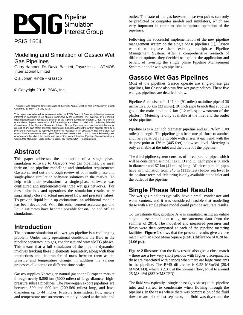
Liquid Estimation from Pressure Drop This method uses the current flow rate to determine the steady

state inventory, by looking this up from the curves shown in

Figure 4. These curves were produced by an offline analysis of

the pipeline.

The second step of this method is to compare the measured

pressure drop along the pipeline to the pressure drop that would

be expected for the current flow rate in steady state. This is done

using the curve from Figure 3, which was produced by an

offline analysis of the pipeline.

How close to steady state the current pipeline values are to

steady state is then estimated by calculating the factor:

SteadyState

SteadyState Linear

P P

P P

With ∆PLinear>=0 the linear pressure drop for the current flow

rate taken from the straight line in Figure 3, this gives a value

α<=1. This factor is then used as a multiplier on the steady state

level from Figure 4 to calculate the estimated pipeline

inventory.

The estimated liquid volume V is given as:

1SteadyState Linear LinearV V V V

The method uses a 10 minute running mean value on pressure

and flow measurement to smooth out inventory peaks. The rate

of change in the liquid inventory cannot exceed the expected

inventory change per time step, thus a dampening factor was

introduced. The maximum allowed growth in the liquid

inventory introduced was:

1n n InV V L F

Where InL F is the liquid dropout rate per time step at the

current inlet flow rate.

In this analysis no limitation on the rate of change has been put

on the amount of liquid out of the pipeline, as this is difficult to

quantify. This would affect the result as the average liquid

volume would be under estimated.

Pipeline C, D and E The test case considers pipeline C in the time period from

01.10.2014 to 31.10.2014. Average outlet pressure is 87.5 barg

(1270 psig).

Figure 5 shows delta pressure with liquid estimation result

from the multiphase model and delta pressure inventory

algorithm. The mean difference between the multiphase model

and liquid estimate is 14.1 m3 (500 ft3) with a standard deviation

of 27.3 m3 (965 ft3).

3 Garry Hanmer, David Basnett, Fayaz Issak, Ola Johan Rinde PSIG 1604

Pipeline B The test for pipeline B, uses data from a start-up period from

10.01.15 to 16.02.15. Note that there is an issue with the

comparison to the multiphase model due to the number of

restarts in the online system. Each time the online multiphase

model has to be restarted, it restarts from a steady state, leading

to a jump in the liquid levels. It would be possible to get a better

set of results if the online data was re-run.

Figure 6 shows the pressure based liquid accumulation in the

test period. The mean difference between the multiphase model

and liquid estimate is 146.4 m3 (5160 ft3) with a standard

deviation of 119 m3 (4200 ft3).

Liquid Estimation from Accumulators Calculating the liquid inventory by using accumulators uses an

equation which converge towards the steady state volume. The

steady state volumes and accumulation rates can be found from

either analysis of the data for the running pipeline, or a steady

state run of a multiphase model. The following simplistic

equation has been used:

11 1 n

n n In

SteadyState In

VV V L F

V F

Where InL F is the total liquid (Water + Condensate)

accumulation rate at the current inlet flow rate and 1nV is the

accumulated liquid volume in the previous time step.

If the inventory is above the steady state level, the liquid level

is updated by:

2

11 1 n

n n In

SteadyState In

VV V L F

V F

Note that now 1SteadyState In nV F V and so this reduces the

accumulated volume.

Water/MEG and Condensate Split The above method provides an estimate of the total liquid

content. It was extended to provide an estimate of the separation

between the Water/MEG and Condensate phase by tracking the

water/MEG as well as the total liquid. For the Water/MEG a

linear accumulation in the pipeline was assumed, giving.

, , 1Water n Water n Water InV V L F

The Water/MEG drainage is assumed as:

, 1

, , 1

,

1Water n

Water n Water n Water In

Water SteadyState In

VV V L F

V F

As with the total liquid estimate, the steady state water/MEG

volumes and accumulation rates required can be found from

either analysis of the data for the running pipeline, or a steady

state run of a multiphase model.

Performance of this SApproach

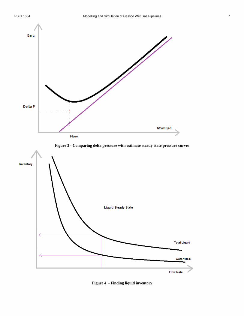
Pipeline C The test case for pipeline C covers the time period from

01.10.2014 to 31.10.2014.

Figure 7 shows values from the multiphase model and liquid

estimation from accumulators. The mean difference between

multiphase model and liquid estimate is 7.3 m3 (258 ft3) with a

standard deviation of 16.4 m3 (580 ft3).

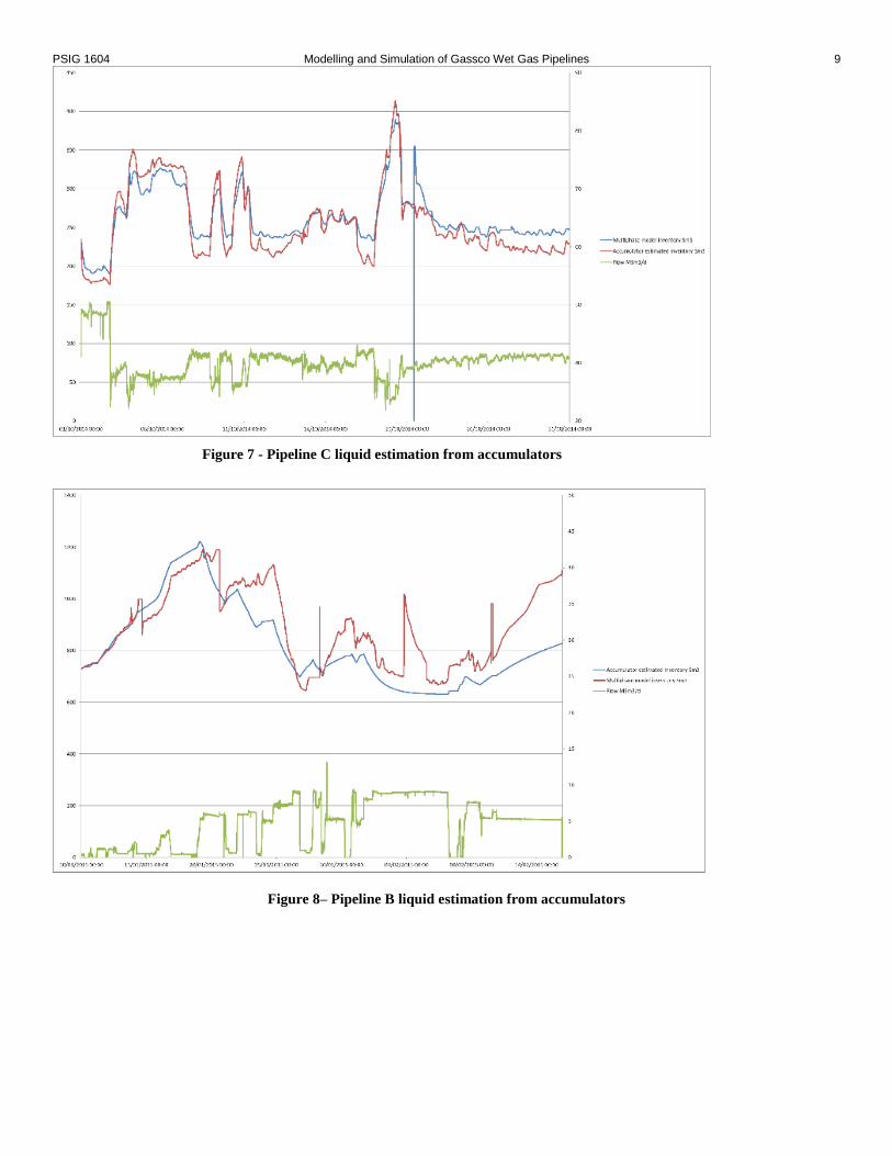
Pipeline B Start-up period from 10.01.15 to 16.02.15 has been used as a

test case for both pressure based and accumulator based liquid

estimation.

Figure 8 shows the result from the liquid accumulator

approach. The mean difference between multiphase model and

liquid estimate is 7.5 m3 (265 ft3) with a standard deviation of

85.1 m3 (3005 ft3). The match for liquid content would be better

if the model had not been cold started as often as it has, since

the model results would not contain the ‘jumps’ from being

restarted.

Investigation Results Pressure drop based liquid estimation gives consistently good

results when the pressure drop is stable. In addition it gives fast

result as it does not use the historical data. The pressure drop

liquid estimation has issues when the pressure drops vary, and

without limiting the rate of change in the results it could become

inaccurate. A drawback of this approach is that pressure

changes not related to the liquid volume could give changes in

liquid inventory results.

Accumulator liquid estimation gives a closer match between the

estimate and multiphase model results than the pressure drop

method. Testing shows that a rough estimate of the separation

between water/MEG and condensate is achievable. The results

of this method should tend towards the correct liquid levels

when the pipeline operates close to steady state.

The result from the tests shows that the accumulator approach

has the greatest potential as water/MEG content can be

estimated.

Chosen Solution Based on the above analysis, it was decided that a solution

based on the liquid estimation from accumulators would

provide the best results.

Some changes were made to the basic algorithms presented

above. For flow rates below a given threshold value, the total

liquid accumulates linearly up to the steady state level, instead

of having a term based on the ratio of estimated steady state

liquid accumulation. This then gives the low flow accumulation

4 Modelling and Simulation of Gassco Wet Gas Pipelines PSIG 1604

as:

1n n InV V L F

Tuning parameters were added for the 4 rates:

1. Total liquid accumulating

2. Total liquid draining

3. Water/MEG accumulating

4. Water/MEG draining

These tuning rates were added as multipliers to the

accumulation rates from the steady state lookup tables. So in

the above equations, wherever InL F appears, this would

be multiplied by the appropriate tuning factor.

Manual tuning of these parameters gave closer agreements with

the multiphase model results than in the original analysis.

To improve the results of the system further, manual tuning of

the accumulation and draining rates were carried out. The

tuning consisted of a simple multiplier applied to the steady

state rates for the current pressure and flow.

Tuning Pipeline C Using the algorithm as described above, and running for the

data from January 2014:

In Figure 9 we can see that the results for the liquid level are in

pretty good agreement. The liquid content accumulates slightly

faster than the estimated results do, and there are a few points

where the results appear to have converged to a “steady state”

level, but the estimated results continue to accumulate.

We can see from the comparison of the water content in Figure

10, the estimator does a far worse job of matching the results.

In particular, the results drain the water far faster than the

estimator when the flow rate changes. This makes it hard to see

whether the accumulation rates are accurate or not, although the

slope of the lines during accumulation are similar.

Based on the observation that the water drains much faster than

the estimator predicts, the water drain expression from the

original approach was replaced with one that uses a linear

model for draining.

The tuning factors for the accumulation and drain rates were

estimated to be.

Liquid Accumulation Factor = 1.5

Liquid Drain Factor = 1.0

Water Accumulation Factor = 1.05

Water Drain Factor = 10.0

For the liquid level, the tuning gives a slightly closer visual

match to the data in Figure 11, although the estimator is now

overshooting on a few of the peaks, rather than undershooting,

suggesting that the liquid accumulation factor may be a little bit

too high, and require further tuning. However the results

already matched pretty well, so the improvement is not

dramatic. Looking at the RMS errors they haven’t really

changed, being about 42 m3 (1483 ft3) in each case.

The changes have made a far more dramatic improvement to

the water content for this data set as seen in Figure 12. The

estimator results are now responding quickly to draining of the

line, in the same way as the source results. It appears that the

drain rate may now be slightly too fast, since the estimator

results overshoot several times, so the water drain factor could

probably be tuned further. Looking at the slopes of the line

when accumulating water, they look similar, so the

accumulation does not need any more tuning. The RMS error

in the water content has been reduced from 42 m3 (1483 ft3) to

25 m3 (882 ft3).

Leak Detection During the model performance evaluation an investigation of

the volume balance accumulators and the deviation between the

metered and modelled pressures and flows was performed.

The volume balance is a calculation of the deviation between

the inlet and outlet flow including the modelled pipeline

inventory as an estimate for changes in the pipeline inventory.

The imbalance calculated by the equation is accumulated over

a running time period and if the value is above a user defined

threshold an alarm is raised.

Typically, the performance was good during periods with stable

production, particularly when the flow rate was high and the

liquid was moving with a constant flow rate out of the pipeline.

When the flow rate was reduced to a low level, liquid starts to

accumulate in the pipeline and less volume exiting the pipeline

than entering at the inlet. The volume balance will then indicate

that the volume is disappearing in the pipeline and it will look

like a leak. This deviation was however small since the amount

of liquid that condensed in the pipeline was small because of a

relatively dry gas at the pipeline inlet.

After shutdowns and the subsequent start-up of the pipeline,

larger deviations between the model and the metered data were

observed. This resulted in a larger deviation in the balance. It is

believed that the increased deviation after shutdowns/start up is

caused by an error in the gas inventory in the pipeline model.

This will give a deviation between the modelled and metered

pressure and flow that influence the leak detection. In some

cases, the deviation could be large for a limited period after the

startup. The error is caused by a different pressure profile in a

dry gas pipeline and a pipeline with liquid. Since the liquid

concentration is higher at the end of the pipeline this led to a

higher pressure drop towards the end of the line. When the

liquid is transported up the riser at the end of the pipeline (or

where it hits land) there is always an additional pressure drop

caused by the liquid transport in the inclined sections. Because

of this, there will be a higher pressure drop in the last half of the

multiphase pipeline than simulated by the single phase model

and the inventory will also be different compared with reality.

To compensate for the model errors caused by the liquid in the

pipeline, a dynamic leak detection threshold functionality was

5 Garry Hanmer, David Basnett, Fayaz Issak, Ola Johan Rinde PSIG 1604

created. This functionality will adjust the leak detection

thresholds according to user-defined settings. Typically, the

thresholds will be increased when there have been large rate

changes in the pipeline that caused changes in the amount of

liquid in the pipeline or after shutdowns where the inventory

errors have an influence on the results.

Two scenarios were considered for enhancing the leak detection

performance of a multi-phase pipeline by using the liquid

estimator described above in combination with single phase

leak detection software. This functionality was not developed,

but could be future work to improve the system.

1. Liquid is accumulating in the pipeline:

The current liquid level is used and compared with the steady

state liquid level. If the difference is greater than a given delta,

the liquid level can be considered to be accumulating, and the

simulated inventory calculations are considered to be degraded.

The sensitivity of the leak detection can then be degraded. 2. Liquid is draining out of the pipeline:

The current liquid level is used and compared with the steady

state liquid level. If the liquid known to be exiting the pipeline

is above a given threshold the sensitivity of the leak detection

can then be degraded.

Once the difference between steady state level and current

liquid level is below a threshold value, the sensitivity can be

returned to normal operating conditions.

Conclusions This paper shows that for the pipelines of interest, accurate

simulation of the pressure and flow in a wet gas pipeline is

possible using suitably tuned single phase simulation software

when online tuning is activated.

It also details the investigation into a simple online system for

estimation of the liquid holdup in these pipelines. The system

produces good results in many circumstances. This has been

validated by comparing the results from the liquid estimator

with the results for liquid holdup from a multiphase simulator

engine.

For future improvement further work could be carried out in the

following areas:

Automate tuning of the accumulation and drain rates

for the liquid estimator to minimize RMS errors. This

would require more data than the current liquid

estimator requires. The target drain and accumulation

rates are not measured directly, and so they would

have to be provided by a multiphase simulation,

suggesting that an offline tool would be required.

As part of the development, the facility was added to

feed the liquid drained from one pipeline as extra

liquid volume to another pipeline. Currently this

injected liquid is added directly to the total liquid

estimate for the current step. It would be possible to

track the injected and accumulated liquids separately.

Since the flow rate is known in the pipeline, an

estimate of the injected liquid flow rate could be

derived from this, and thus estimating the arrival time

of the injected fluid at the outlet of the pipeline. This

would require further investigation to assess the

feasibility and accuracy of such an approach.

REFERENCES 1. Ben Velde, Willy Postvoll, Garry Hanmer, James

Munro, “Application Benefit of the Online Simulation

Software for Gassco’s Subsea Pipeline Network”,

PSIG Annual Meeting held in Prague, Czech

Republic, 16 April – 19 April 2013.

Author Biography Garry Hanmer is a Principal Project Engineer at ATMOS

International in Manchester, United Kingdom. Garry Hanmer

has over 10 years’ experience in the pipeline industry with an

emphasis on pipeline hydraulic simulation. He also has

experience in development and delivery of pipeline operations

and integrity management software systems. Garry Hanmer has

a Master of Engineering in Aeronautical Engineering (MEng

Hons) from the University of Salford, UK.

Dr. David Basnett is the Chief Scientist at Atmos International,

where he has been developing pipeline application software for

more than 13 years, specializing in simulation. David has a

degree in Mathematics from Cambridge University UK, and a

PhD from UMIST UK, he is registered as a Chartered

Mathematician with the Institute of Mathematics and its

Applications.

Fayaz Issak is a senior software engineer and project manager

at Atmos International in Manchester, UK. He has 10 years’

experience in the pipeline industry, working in risk analysis,

pipeline operations, leak detection, pipeline simulation and

pipeline management systems. Fayaz has a Bachelor of Science

in Computer Science from the University of Salford and is

Microsoft and Prince2 Certified.

Ola Johan Rinde has a Master of Science in mechanical

engineering at NTNU in Norway with specialization on wet gas

compressing. Ola has worked for 5 years in the Polytec R&D

foundation and 9 years in Gassco. Ola has mainly worked on

multiphase pipeline operation and development of online single

and multiphase simulation systems.

FIGURES

Figure 1 - Measured and modelled pressure at outlet of pipeline A

Figure 2 - Measured and modelled flow at outlet of pipeline A

PSIG 1604 Modelling and Simulation of Gassco Wet Gas Pipelines 7

Figure 3 - Comparing delta pressure with estimate steady state pressure curves

Figure 4 - Finding liquid inventory

8 PSIG 1604 Garry Hanmer, Dr. David Basnett, Fayaz Issak - ATMOS International Limited, Ola Johan Rinde – Gassco

Figure 5– Pipeline C liquid estimation from pressure

Figure 6– Pipeline B liquid estimation from pressure

PSIG 1604 Modelling and Simulation of Gassco Wet Gas Pipelines 9

Figure 8– Pipeline B liquid estimation from accumulators

Figure 7 - Pipeline C liquid estimation from accumulators

10 PSIG 1604 Garry Hanmer, Dr. David Basnett, Fayaz Issak - ATMOS International Limited, Ola Johan Rinde – Gassco

Figure 9 – Pipeline C un-tuned liquid estimation

Figure 10 – Pipeline C untuned water estimation

PSIG 1604 Modelling and Simulation of Gassco Wet Gas Pipelines 11

Figure 11 - Pipeline C tuned liquid estimation

Figure 12 - Pipeline C tuned water estimation