Simulation of Anchor Loads on Pipelines - NTNU Open
129
Simulation of Anchor Loads on Pipelines Kristbjörg Edda Jónsdóttir Marine Technology Supervisor: Svein Sævik, IMT Department of Marine Technology Submission date: June 2016 Norwegian University of Science and Technology
-
Upload
khangminh22 -
Category
Documents
-
view
2 -
download
0
Transcript of Simulation of Anchor Loads on Pipelines - NTNU Open

Simulation of Anchor Loads on Pipelines
Kristbjörg Edda Jónsdóttir
Marine Technology
Supervisor: Svein Sævik, IMT
Department of Marine Technology
Submission date: June 2016
Norwegian University of Science and Technology


MASTER PROJECT WORK SPRING 2016
for
Stud. tech. Kristbjörg Jónsdóttir
Simulation of anchor loads on pipelines Simulering av ankerlaster på rørledninger
Anchor loads on pipelines is in general a rarely occurring event, however, the severity when it
occurs could easily jeopardize the integrity of any pipeline. It is considered as an accidental
load in the design of pipelines. In the Norwegian Sea there are several locations where the
subsea pipeline density is high, also in combination with high vessel density. The vessels
usually know where pipelines are located and avoid anchoring, but anchors might be dropped
in emergencies, lost in bad weather or due to technical failures. In these cases, the drop might
not be noticed before the anchor hooks, e.g. in a pipeline.
The master thesis work is to be carried out as a continuation of the project work as follows:
1. Literature study on pipeline technology, relevant standards for pipeline design, with
particular focus on impact loads. Aspects related to vessel size, frequencies and
corresponding anchor equipment is to be included also using previous thesis by Wei
Ying and Stian Vervik as starting points.
2. Study the theoretical background for and get familiarized with the computer program
SIMLA
3. Define the basis for a case study considering anchor geometry, pipeline mechanical
properties, soil interaction parameters, wire chain capacity, water depth, friction and
hydrodynamic coefficients
4. Establish SIMLA models for the hooking event that allows for sliding under friction
along the pipeline and perform simulations to demonstrate the performance of the
model.
5. Then perform parametric studies in order to categorize the anchor contact behaviour as
follows:
a. Assume two pipe diameters 30 inch and 40 inch with D/t = 35
b. Assume ship velocities 2 knots and 10 knots
c. Look at the anchor chain lengths and identify contact scenarios as a function of
water depth for three water depths
d. Assume the pipe to be continuously supported and identify hooking scenarios
for tow direction/pipeline relative angles 90, 60 and 30 deg (using a stiff model).
e. Based on identified hooking scenarios, make a refine FE model to study the
overall detailed behaviour including the pipeline global response.
6. Conclusions and recommendations for further work
All necessary input data are assumed to be delivered by Statoil.
The work scope may prove to be larger than initially anticipated. Subject to approval from the
supervisors, topics may be deleted from the list above or reduced in extent.
In the thesis the candidate shall present his personal contribution to the resolution of problems
within the scope of the thesis work

Theories and conclusions should be based on mathematical derivations and/or logic reasoning
identifying the various steps in the deduction.
The candidate should utilise the existing possibilities for obtaining relevant literature.
Thesis format
The thesis should be organised in a rational manner to give a clear exposition of results,
assessments, and conclusions. The text should be brief and to the point, with a clear language.
Telegraphic language should be avoided.
The thesis shall contain the following elements: A text defining the scope, preface, list of contents,
summary, main body of thesis, conclusions with recommendations for further work, list of symbols
and acronyms, references and (optional) appendices. All figures, tables and equations shall be
numerated.
The supervisors may require that the candidate, in an early stage of the work, presents a written
plan for the completion of the work.
The original contribution of the candidate and material taken from other sources shall be clearly
defined. Work from other sources shall be properly referenced using an acknowledged referencing
system.
The report shall be submitted electronically on DAIM:
- Signed by the candidate
- The text defining the scope included
- In bound volume(s)
- Drawings and/or computer prints which cannot be bound should be organised in a
separate folder.
Ownership
NTNU has according to the present rules the ownership of the thesis. Any use of the thesis has
to be approved by NTNU (or external partner when this applies). The department has the right
to use the thesis as if the work was carried out by a NTNU employee, if nothing else has been
agreed in advance.
Thesis supervisors:
Prof. Svein Sævik, NTNU
Dr. Erik Levold, Statoil
Deadline: June 10, 2016
Trondheim, January, 2016
Svein Sævik
Candidate – date and signature:

i
Preface
This thesis is based on research carried out during the spring semester of 2016 at the Department
of Marine Technology, NTNU, as part of my Master’s degree in Marine Technology, with
Underwater Technology as specialization. The thesis is a continuation on the work I carried out
during the autumn semester of 2015 in the course TMR4580: Marine Subsea Engineering,
Specialization Project.
The main topic of this thesis is to inspect how and which parameters affect anchor-pipeline
interaction through simulation of the interaction using the computer software SIMLA. This was
done by carrying out a parameter study and eleven case studies.
This thesis is a continuation of Master theses by Stian Vervik (2011) and Ying Wei (2015). The
initial SIMLA input files were received from Wei (2015). A large amount of time has gone into
understanding these input files and modifying them, as old drafts were received for the
parametric study. Modifying and updating the input files was by far the most time consuming
part of this thesis. The scope of the thesis was narrowed compared to the work description
presented above, by altering point 5 C). Only one water depth was investigated to determine
the minimum anchor length for interaction.
I would like to thank my supervisor Prof. Svein Sævik at the Department of Marine Technology,
NTNU, for his guidance during this project with regards to theoretical understanding and the
computer software SIMLA. I would also like to thank Dr. Erik Levold from Statoil for the input
parameters, and I would like to acknowledge MARINTEK regarding the license of SIMLA.
Lastly, a special thanks to my parents and the girls in office A2.027 for help with the thesis.
Trondheim, June 2016
Kristbjörg Edda Jónsdóttir


iii
Summary
Incidents where anchor and pipeline interact are rare, but such an event can have drastic
consequences. In the report, Pipeline and Riser Loss of Containment by HSE, published in 2001
for the UK sector, 44 incidents involving anchors and pipelines were found for the period
1990-2000. Furthermore, The International Cable Protection Committee reported that between
2007-2008, there were ten cases of submarine cables damaged due to anchor damage. All of
these cases were due to vessels being unaware of their anchors being deployed during transit.
The objective of this thesis is to study the anchor’s and the pipeline’s response to such
interactions. The response of the anchor was investigated by performing a parametric study and
categorizing the anchor’s behaviour. The pipeline was modelled as a 10 meter long constrained
rigid body in this study. The literature usually defines anchor behaviour as impact, hooking or
pull over. In this study a new system was made for the categorization of the behaviour. The
behaviour was either categorized as brief or lasting contact. If categorized as brief, the contact
was further defined as either pull over or bounce over. If lasting contact, it was defined either
as hooking or sliding, with or without twisting.
Seventy-eight models were analysed in the parametric study. The parameters investigated were
the anchor’s mass and geometry, towing speed of the anchor, size of pipeline and angle of attack
between anchor and pipeline. Forty-eight new models were created to investigate the minimum
chain length for the towed anchor to reach the subsea pipeline. A constant water depth of 200
meters was applied in all studies.
The pipeline’s global response was studied by performing eleven case studies. The parameters
applied in these cases were based on the results from the parametric study and the minimum
chain length study. In the eleven cases studied, the pipeline was modelled to be 10 kilometer
long, with elastoplastic material properties. The pipeline was constrained at the ends, but
otherwise allowed to displace and globally deform. The effect of the interaction on the pipeline
was investigated by studying the longitudinal strains in the cross-section. The results were

iv
compared with DNV’s design load strain for combined loading, and with the pipeline’s
characteristic strain resistance.
The study of minimum chain length revealed that for an anchor towed at 2 knots, a chain length
approximately 3 meters longer than the water depth was required. For the 10 knot case, due to
drag forces, the chain needed to be roughly 110 meters longer than the water depth. However,
these results are only valid when the anchor is dropped 100 meters away from the pipeline.
The general trend of the anchor behaviour seen in the parametric study, points towards an
increase in hooking and sliding with increased mass of anchor, smaller pipe diameter and lower
vessel speed. The largest amount of hooking scenarios in the parametric study occurred for 60
degrees angle of attack, as the anchor twisted and hooked. No hooking occurred for the 30
degrees cases, while all sliding events occurred for this angle.
Three of the eleven case studies resulted in hooking. In all of these cases, the longitudinal strain
in the cross-section of the pipeline exceeded both DNV’s design load criteria for combined
loading and the pipeline’s characteristic strain resistance. Exceeding the characteristic strain
resistance puts the integrity of the structure at risk for local buckling. However, a more detailed
FEA is necessary to determine the actual response of the cross-section, and which failure
mechanisms it may initiate.
In the case studies with the full-length pipeline, no hooking was obtained for the attack angle
of 60 degrees, which contradicts the results from the parametric study. This may indicate that
the rigid modelling of the pipeline, rather than the anchor’s response, caused the hooking
response in the parametric study.
The three of the eleven case studies that resulted in hooking, revealed that the global
displacement of the pipeline is much greater when the anchor is towed at a lower velocity. For
higher velocities, the hooking case with minimum chain length displaced the pipeline farther,
both laterally and vertically, than the anchor towed with maximum chain length.

v
Sammendrag
Ulykker hvor undersjøiske rørledninger blir utsatt for ankerlaster er sjeldne, men kan ha
dramatiske konsekvenser. Ulykker som Kvitebjørn gassrør-ulykken i 2007, kombinert med den
økende skipstrafikken over rørledninger i Nordsjøen, gjør ankerinteraksjon med rørledninger
til et svært relevant tema.
Formålet med denne oppgaven er å analysere responsen ved interaksjon mellom anker og
rørledning. For å undersøke ankerresponsen, ble en parameterstudie utført. Syttiåtte modeller
ble analysert for å undersøke effekten av ankermasse og -geometri, størrelse på rørledning,
ankerets angrepsvinkel og tauehastighet. Ved undersøkelse av ankerets respons ble
rørledningen modellert som et 10 meter langt fastinnspent stivt legeme.
Tradisjonelt blir interaksjonen mellom anker og rørledning beskrevet som «impact», «hooking»
eller «pull over». Basert på denne terminologien ble et nytt system utviklet og brukt for å
kategorisere interaksjon. Ankerets adferd ble først kategorisert basert på om kontakten mellom
ankeret og rørledninger var kort- eller langvarig. Hvis den var kortvarig, ble den videre definert
som enten «pull over» eller «bounce over». Om kontakten var langvarig, ble den kategorisert
som enten «hooking» og «sliding», med eller uten vridning.
Etter å ha kategorisert adferden til ankeret ble 48 modeller laget for å undersøke effekten av
tauehastighet på ankerkjetting med ulik lengde. Formålet med disse 48 analysene var å definere
minimum lengde på ankerkjettingen for at ankeret skal treffe rørledningen på 200 meters dyp.
DNVs kriteria for maksimal tøyning hvis en rørledning er utsatt for kombinerte laster, har blitt
benyttet for å bedømme rørledningens respons. Hvis tøyningen i tverrsnittet overskrider denne
verdien, kan lokal knekking oppstå. Elleve casestudier ble opprettet på grunnlag av funn fra
parameterstudiet og studiet av minimum lengde på ankerkjetting. I casestudiene ble
rørledningen modellert som 10 kilometer lang med elastoplastiske material egenskaper, kun
fastinnspent ved endene.

vi
Minimum lengde på ankerkjetting for at ankeret skal treffe et rør på 200 meters dyp, er avhengig
av tauehastigheten. Resultatene viste at ved lav hastighet, 2 knot, må kjettingen være minst 3
meter lengre enn vanndybden for at ankeret skal treffe røret. Ved høy hastighet, 10 knot, må
kjettingen være minst 110 meter lengre enn vanndybden. Disse resultatene er kun gyldige hvis
ankeret starter maksimalt 100 meter unna røret.
Resultatene fra parameterstudiet viser en økning i «hooking»- og «sliding»-responser ved økt
ankermasse, lavere tauehastighet og mindre diameter på rørledningen. Flertallet av
interaksjonene som resulterte i en «hooking»-respons, forekom når angrepsvinkelen var 60
grader. «Sliding» forekom kun når angrepsvinkelen var 30 grader.
Tre av de elleve casestudiene resulterte i «hooking». I disse overskred den langsgående
tøyningen i tverrsnittet DNV’s kriteria for tillatt tøyning, og rørets karakteristiske
tøyningsmotstand. Dette setter rørledningens tverrsnitt i fare for lokal knekking.
Det forekom ingen «hooking»-respons i casestudiet når angrepsvinkel var 60 grader. Dette kan
indikere at «hooking»-responsen i parameterstudiet var forårsaket av hvordan rørledningen ble
modellert, og ikke av ankerets respons.
Fra casestudiene som resulterte i «hooking» er det tydelig at den globale forskyvningen av
rørledningen er større når ankeret taues ved lavere hastighet. For casene med høyere hastighet,
ble rørledninger forskjøvet lengre lateralt og vertikalt når ankeret ble tauet med kortest mulig
ankerkjetting.
vii
Table of Contents
Preface ........................................................................................................................................ i
Summary .................................................................................................................................. iii
Sammendrag ............................................................................................................................. v
List of Figures .......................................................................................................................... xi
List of Tables .......................................................................................................................... xiii
Nomenclature .......................................................................................................................... xv
1 Introduction ........................................................................................................................ 1
1.1 Motivation .................................................................................................................... 1
1.2 Objective ...................................................................................................................... 2
1.3 Scope and limitations ................................................................................................... 2
1.4 Outline of Thesis .......................................................................................................... 3
2 Anchor-Pipeline Interaction .............................................................................................. 5
2.1 Subsea Pipelines ........................................................................................................... 6
2.2 Anchors ........................................................................................................................ 7
3 Rules, Regulations and Literature Review ..................................................................... 11
3.1 DNV Rules and Regulations ...................................................................................... 11
3.1.1 DNV-OS-F101 ................................................................................................ 12
3.1.2 DNV-OS-E301................................................................................................ 15
3.1.3 DNV-RP-F111 ................................................................................................ 17
3.2 Research Papers ......................................................................................................... 17
3.3 Master theses .............................................................................................................. 20
3.3.1 “Pipeline Accidental Load Analysis” ............................................................. 20
3.3.2 “Anchor Loads on Pipelines” ......................................................................... 22
4 Non-linear Finite Element Analysis ................................................................................ 25
4.1 Basics of Finite Element Method ............................................................................... 26
4.1.1 Equilibrium ..................................................................................................... 26

viii
4.1.2 Kinematic Compatibility................................................................................. 27
4.1.3 Constitutive Equations .................................................................................... 28
4.2 Co-rotational Total Lagrangian Formulation ............................................................. 30
4.3 Solution Methods ....................................................................................................... 32
4.3.1 Static Solution ................................................................................................. 32
4.3.2 Dynamic Solution ........................................................................................... 33
5 Modelling ........................................................................................................................... 37
5.1 SIMLA ....................................................................................................................... 39
5.2 Pipe Elements ............................................................................................................. 40
5.2.1 Anchor ............................................................................................................ 41
5.2.2 Chain ............................................................................................................... 43
5.2.3 Pipeline ........................................................................................................... 43
5.3 Contact elements ........................................................................................................ 44
5.3.1 Contact between physical objects ................................................................... 45
5.3.2 Contact with seabed ........................................................................................ 46
5.4 Environmental conditions and other parameters ........................................................ 47
5.5 Specifics of Analyses ................................................................................................. 48
5.5.1 Parametric study ............................................................................................. 48
5.5.2 Minimum Chain Length.................................................................................. 49
5.5.3 Elastoplastic Case Studies .............................................................................. 51
6 Results and Discussion ..................................................................................................... 53
6.1 Parametric Study ........................................................................................................ 53
6.1.1 Results ............................................................................................................. 56
6.1.2 Discussion ....................................................................................................... 61
6.2 Minimum Chain Length ............................................................................................. 64
6.2.1 Results ............................................................................................................. 65
6.2.2 Discussion ....................................................................................................... 66
6.3 Elastoplastic Case Studies .......................................................................................... 68
6.3.1 Results ............................................................................................................. 69
6.3.2 Discussion ....................................................................................................... 71
7 Conclusion ......................................................................................................................... 75
8 Further Work .................................................................................................................... 77
Bibliography ........................................................................................................................... 79
Appendix .................................................................................................................................... I
Appendix A Alterations done to Wei’s Model for Parametric Study ................................ I
Appendix B Structure of MATLAB scripts ..................................................................... V
Appendix C Calculations for Pipe Elements................................................................... IX

ix
Appendix D Results from the Parameter Study ............................................................ XV
Appendix E Results from Elastoplastic Case Studies .................................................. XIX
Appendix F MATLAB scripts and Input Files ........................................................ XXVII


xi
List of Figures
Figure 2.1: Stress components in cross-section segment of the pipewall (Sævik, 2014)........... 6
Figure 2.2: Spek anchor (SOTRA, 2014a) ................................................................................. 8
Figure 2.3: SOTRA Chain (SOTRA, 2014b) ............................................................................. 9
Figure 3.1: Definition of safety classes (DNV-OS-F101, 2013) .............................................. 12
Figure 3.2: Typical link between scenarios and limit states (DNV-OS-F101, table 5-8) ........ 14
Figure 3.3: Load effect factor combinations (DNV-OS-F101, table 4-4) ................................ 14
Figure 3.4: Part of the table describing equipment requirements (DNV-OS-E301) ................ 16
Figure 3.5: Distribution of the 237 vessels which cause hooking, figure by Vervik (2011) ... 21
Figure 4.1: Stress-strain showing elastic and plastic strain contribution (Moan, 2003b) ........ 28
Figure 4.2: Kinematic and isotropic hardening (Moan, 2003b) ............................................... 30
Figure 4.3: Global (I), nodal (i) and element base (j) vector (Sævik, 2008) ........................... 31
Figure 4.4: Modified Newton-Raphson iterations (Moan, 2003b) ........................................... 33
Figure 5.1: All components needed to model the interaction, with coordinate system ........... 37
Figure 5.2: Angle of attack between pipeline and anchor ........................................................ 38
Figure 5.3: Naming system ...................................................................................................... 38
Figure 5.4: Naming system for required anchor chain length .................................................. 39
Figure 5.5: Overview over modules from SIMLAs user manual (Sævik et al., 2010) ............ 40
Figure 5.6: Simplified geometry seen above and from the side ............................................... 41
Figure 5.7: Anchor modelled seen in XPost ............................................................................ 42
Figure 5.8: Complete model in the required anchor chain length study .................................. 50
Figure 6.1: Simulation snapshots of realistic pull over response ............................................. 54
Figure 6.2: A realistic bouncing off response .......................................................................... 54
Figure 6.3: Two realistic cases of hooking, (a) without twisting and (b) with twisting .......... 54
Figure 6.4: Sliding with twist and pull over response .............................................................. 55
Figure 6.5: Summary of categorisation .................................................................................... 55
Figure 6.6: Ratio for hooking, sliding and bouncing off .......................................................... 57
Figure 6.7: Distribution of Brief Contact Ratio seen in Figure 6.6 .......................................... 57

xii
Figure 6.8: Hooking ratio depending on angle of attack and anchor mass .............................. 58
Figure 6.9: Sliding ratio depending on angle of attack and anchor mass ................................. 59
Figure 6.10: Hooking ratio depending on pipe size and vessel velocity .................................. 60
Figure 6.11: Sliding ratio depending on pipe size and vessel velocity .................................... 60
Figure 6.12: Snapshots showing the effect of size and velocity on attack point ...................... 62
Figure 6.13: Error in nodal velocities in Y- and Z-direction ................................................... 64
Figure 6.14: Chain shape for different lengths after 70 seconds with 2 knot velocity ............. 65
Figure 6.15: Chain shape for different lengths after 70 seconds with 10 knot velocity ........... 66
Figure 6.16: Simplified assumption of geometry for two anchor chain coordinates ............... 67
Figure 6.17: Initial configuration of 15400kg200m30in2kn660m90 ....................................... 69
Figure 6.18: Maximum displacement before reaching chain break load ................................. 69
Figure 6.19: Gauss points on the cross-section ........................................................................ 70
Figure 6.20: Element force in anchor chain element 50002 .................................................... 72 Figure B.1: Structure of MATLAB script, parametric study ................................................... VI
Figure B.2: Structure of MATLAB scripts, minimum chain length study ........................... VIII
Figure C.1: Simplified Anchor Geometry ................................................................................ IX
Figure E.1: Plots for 9900kg200m30in2kn660m90 & 9900kg200m30in10kn660m90 ........ XX
Figure E.2: Plots for 9900kg200m40in2kn660m90 & 9900kg200m30in2kn660m60 ......... XXI
Figure E.3: Plots for 15400kg200m30in2kn743m90 & 15400kg200m30in10kn743m90 .. XXII
Figure E.4: Plots for 15400kg200m40in2kn743m90 & 15400kg200m30in10kn743m60 XXIII
Figure E.5: Plots for 15400kg200m30in10kn350m90 ....................................................... XXIV
Figure E.6: Plots for 15400kg200m30in10kn350m60 & 15400kg200m30in10kn350m30 XXV

xiii
List of Tables
Table 1.1: Given parameters from Statoil .................................................................................. 3
Table 2.1: Dimensions in Figure 2.2 for different anchor masses (SOTRA, 2014a) ................. 8
Table 3.1: Equipment letter and class in Vervik’s (2011) thesis ............................................. 20
Table 3.2: Parameters inspected by Wei (2015)....................................................................... 23
Table 5.1: General properties applied in the analyses .............................................................. 38
Table 5.2: Important pipeline parameters ................................................................................ 44
Table 5.3: Parameters investigated ........................................................................................... 48
Table 5.4: Parameters investigated in chain length versus depth ............................................. 50
Table 5.5: Parameters studied in the elastoplastic study .......................................................... 51
Table 5.6: Complete list of analyses carried out in the elastoplastic study .............................. 51
Table 6.1: Overview of usable results in parametric study ...................................................... 56
Table 6.2: List of inconclusive models .................................................................................... 56
Table 6.3: Response ratios for different anchor sizes .............................................................. 58
Table 6.4: Hooking ratio distribution for all parameters, excluding 30 degrees ...................... 59
Table 6.5: Sliding ratio distribution for all parameters excluding, 60 and 90 degrees ............ 60
Table 6.6: Final Z-coordinate for chain element connected to anchor with 2 knots ................ 65
Table 6.7: Final Z-coordinates for chain element connected to anchor with 10 knots ............ 66
Table 6.8: Minimum required anchor chain length .................................................................. 67
Table 6.9: Calculation of characteristic bending strain resistance ........................................... 68
Table 6.10: Overview of usable results in elastoplastic study ................................................. 70
Table 6.11: Summary of results in Elastoplastic Study ........................................................... 71
Table 6.12: Global displacement of roller element .................................................................. 71 h Table C.1: Anchor calculations ................................................................................................. X
Table C.2: Cable calculations ................................................................................................... XI
Table C.3: Pipeline calculations .............................................................................................. XII
Table D.1: Parameter study results ........................................................................................ XV

xiv
Table E.1: Results for the cases studied ................................................................................ XIX
Table F.1: Content of electronical Appendix F, uploaded to DIVA ................................. XXVII

xv
Nomenclature
Abbreviations
𝐴𝐿𝑆 Accidental Limit State
DNV Det Norske Veritas
FEA Finite Element Analysis
FEM Finite Element Method
FLS Fatigue Limit State
HSE Health and Safety Executive (UK)
MARINTEK Norwegian Marine Technology Research Institute
SLS Serviceability Limit State
ULS Ultimate Limit State
Roman Letters
Unfortunately many of the same roman letters have been used for more than one purpose, the
exact meaning of each letter is therefore explained in the text.
𝑎1 Fluid acceleration
A Area
A Projected area
c Damping
ccritical Critical damping
C Impulse shape factor
C Damping matrix
C0 Diagonal damping matrix
𝐶𝑀 Mass coefficient
𝐶𝐷 Drag coefficient
D Outside diameter
E Young’s modulus

xvi
E Green strain tensor
Ee Elastic strain tensor
Ep Plastic strain tensor
EN Equipment number
𝑑𝐹ℎ𝑜𝑟𝑖𝑧𝑜𝑛𝑡𝑎𝑙 Horizontal forces
𝑑𝐹𝑖𝑛𝑒𝑟𝑡𝑖𝑎 Inertia forces
𝑑𝐹𝑑𝑟𝑎𝑔 Drag forces
𝑓0 Initial ovality
𝑓𝑐 Characteristic material strength
f Related volume force vector
F Maximum impact load
𝐹𝑙𝑖𝑓𝑡 Lift force
F Deformation gradient
I Second moment of inertia
I Impulse load
K Stiffness matrix
L Length of cylinder
𝐿𝑖 Load effects
𝐿𝑆𝑑 Design load
m Mass
M Mass damping matrix
𝑝𝑏 Bursting pressure
𝑝𝑐 Collapse pressure
𝑝𝑒 External pressure
𝑝𝑚𝑖𝑛 Minimum external pressure
r Displacement
𝑅𝑅𝑑 Design resistance
R Load vector
RI Internal force
RE External force
S 2nd Piola-Kirchhoff stress tensor
t Traction on the volume surface
𝑡2 Wall thickness corrected for corrosion
𝑡𝑐 Characteristic thickness
td Duration of impact
xvii
𝑢 Fluid velocity
𝑢𝑥 Displacement in X-direction
𝑢𝑦 Displacement in Y-direction
𝑢𝑧 Displacement in Z-direction
u Displacement
δu Virtual displacement
v0 Initial velocity
vi Velocity at time i
Greek Letters
α1 Mass damping ratio
α2 Stiffness damping ratio
𝛼ℎ Train hardening
𝛼𝑔𝑤 Girth weld factor
γi Load effect factor
γm Material resistance factors
γSC Safety class resistance factor
𝛾𝜀 Strain resistance factor
Δ Displacement
δε Virtual natural strain
휀𝑐 Characteristic bending strain resistance
휀𝑆𝑑 Design loads strain
𝜃𝑥 Rotation about X-axis
𝜃𝑦 Rotation about Y-axis
𝜃𝑧 Rotation about Z-axis
κ Strain-hardening parameter
𝜉 Damping ratio
ρ Density
ρ0 Density of undeformed configuration
σ Natural stress tensor
σ0 Initial stress tensor
σe Von Mises stress
σxx Longitudinal stress
σφφ Hoop stress


1
Chapter 1
1 Introduction
1.1 Motivation
Incidents where anchor and pipeline interact are rare, but can have drastic consequences. In the
report Pipeline and Riser Loss of Containment published in 2001 for the UK sector, 44 incidents
involving anchors and pipelines were found for the time period 1990-2000 (HSE, 2009). The
largest amount of incidents occurred near offshore platforms, followed by incidents further than
100 meters from the platform (HSE, 2009). Eighteen of the incidents were caused by supply
boats, and eleven by construction vessels. The International Cable Protection Committee could
also report that between 2007-2008 ten submarine cables were damaged due to anchor damage
in the UK sector (Damage to Submarine Cables Caused by Anchors, 2009). In all of these cases,
the vessels were unaware that their anchors were deployed during transit.
An example of an anchor-pipeline accident in the Norwegian sector, is the Kvitebjørn gas
pipeline incident (Gjertveit, Berge, & Opheim, 2010). During inspection in 2007, it was
discovered that the pipeline had been dented and local buckling had occurred. It was concluded
that this was due to impact with an anchor as an overwhelming amount of evidence was found,
including a 10 ton anchor retrieved beside the pipeline (Gjertveit et al., 2010).
Despite the small amount of interactions, the consequences of these and the increasing amount
of pipelines and ship traffic across these in the North Sea, makes the topic of anchor-pipeline
interaction highly relevant. Additionally, there is currently a limited coverage of anchor hazards
within both UK Codes/Standards and other publicly available guidance (HSE, 2009).

Chapter 1 Introduction 2
1.2 Objective
There is limited literature regarding anchor-pipeline interaction, however most of this literature
classify the interaction as either: impact, hooking or pull over. This classification may prove to
be somewhat simplistic, and cause loss of information regarding the behaviour of the anchor
and the pipeline’s response. This thesis therefore attempts to categorize and analyse the anchors
behaviour when exposed to different parameters, but also to improve the categorization of the
behaviour. Understanding the anchors behaviour, may increase the knowledge about the
pipeline’s response to the interaction.
Once having determined how the parameters affect the anchor’s behaviour, it is of interest to
inspect the pipeline’s response to the different behaviours, and to determine the consequences
of such an event. The main objective here is to investigate whether the strain in the pipeline’s
cross-section exceeds DNV’s criteria for the characteristic bending strain and design load.
Exceeding this value indicates that the pipeline’s cross-section may experience local buckling
(DNV-OS-F101, 2013).
1.3 Scope and limitations
The master (MA) theses by Vervik (2011) and Wei (2015) create the foundation for this master
thesis. Vervik (2011) studied the likelihood of hooking for the Kvitebjørn gas pipeline and the
impact of anchor hooking on the pipeline. Wei (2015) investigated the effect of parameters on
the probability of hooking and the pipeline’s global response.
To study the interaction, a Finite Element Analysis (FEA) needs to be carried out. To do this
MARINTEK’s software SIMLA was chosen, as it was applied by both Vervik (2011) and Wei
(2015). A draft for the input file used in Wei’s (2015) parametric study, and the input files for
the model including elastoplastic materials, were received by Wei (2015). These input files
were modified and used to study the anchor’s and pipeline’s response to an interaction.
Statoil defined the parameters that are of interest in the attached work description to be: pipe
size, anchor size, anchor chain length, water depth, vessel speed and angle of attack between
anchor and pipeline. The given parameters are summarized in Table 1.1.

Chapter 1 Introduction 3
Table 1.1: Given parameters from Statoil
Pipe Diameter
[Inches]
Vessel velocity
[Knots]
Angle of Attack
[Degrees]
30 2 90
40 10 60
30
A parameter study was performed to determine which combination of parameters cause
hooking, sliding and pull over, and by improving the categorization, get a better impression of
the anchors’ behaviour. The scope of the thesis is narrowed by only inspecting six different
anchor sizes and only one water depth.
Due to time limitations and the complexity of the topic, modelling of the soil has been simplified
quite extensively. The seabed is also modelled as completely flat. The local response of the
pipeline is not studied, as that would require a more detailed analysis.
The scope of the thesis was also narrowed by inspecting only one water depth of 200 meters.
This choice had particular significance for point 5 C) in the attached work description presented
at the beginning of the thesis. The water depth was not altered in the second study, which
investigates the minimum chain length for the anchor to reach the subsea pipeline, when towed.
Instead, the chain’s length was varied.
1.4 Outline of Thesis
Before describing the modelling of the anchor-pipeline interaction, an overview of the problem
is presented through a brief introduction to anchor-pipeline interaction, subsea pipelines and
anchors in Chapter 2.
Relevant literature in the form of rules and regulations by DNV, scientific papers, and the two
master thesis by Vervik (2011) and Wei (2015) are reviewed in Chapter 3.
Non-linear finite element theory used in the SIMLA software to analyse the interaction are
reviewed in Chapter 4.
To inspect the anchor’s and pipeline’s response to an interaction, two main analysis were
carried out. The first, to determine the anchor’s response, was the parametric study, which was
divided into two segments. The first segment inspects all parameters, except the anchor chain
length and depth, and the second segment only inspects only chain length and depth. The second

Chapter 1 Introduction 4
analysis, to study the pipeline’s global response, consists of eleven case studies. The eleven
cases were created based on results from the two previous studies, and investigates the strain in
the pipeline’s cross-section. A description of these analyses, the modelling of the interaction
and calculations procedures are presented in Chapter 5.
Results and discussion for each of the analyses are presented in Chapter 6. The conclusion of
the thesis is presented in Chapter 7, and lastly, further work is discussed in Chapter 8.
5
Chapter 2
2 Anchor-Pipeline Interaction
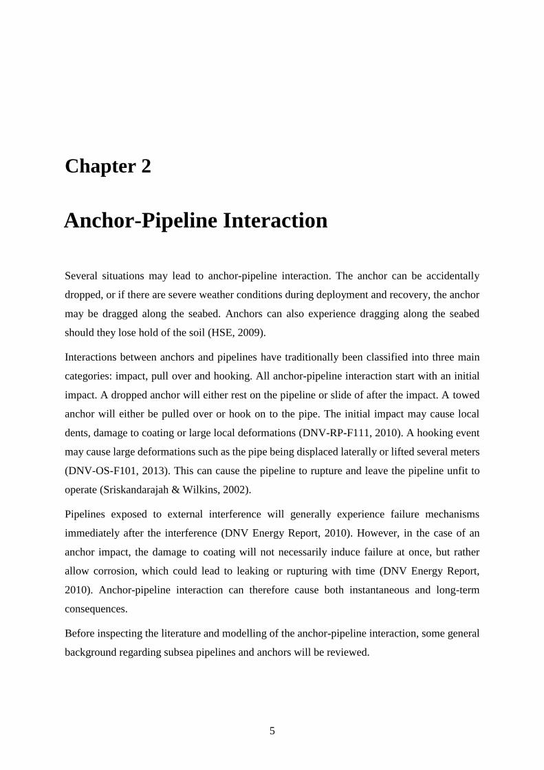
Several situations may lead to anchor-pipeline interaction. The anchor can be accidentally
dropped, or if there are severe weather conditions during deployment and recovery, the anchor
may be dragged along the seabed. Anchors can also experience dragging along the seabed
should they lose hold of the soil (HSE, 2009).
Interactions between anchors and pipelines have traditionally been classified into three main
categories: impact, pull over and hooking. All anchor-pipeline interaction start with an initial
impact. A dropped anchor will either rest on the pipeline or slide of after the impact. A towed
anchor will either be pulled over or hook on to the pipe. The initial impact may cause local
dents, damage to coating or large local deformations (DNV-RP-F111, 2010). A hooking event
may cause large deformations such as the pipe being displaced laterally or lifted several meters
(DNV-OS-F101, 2013). This can cause the pipeline to rupture and leave the pipeline unfit to
operate (Sriskandarajah & Wilkins, 2002).
Pipelines exposed to external interference will generally experience failure mechanisms
immediately after the interference (DNV Energy Report, 2010). However, in the case of an
anchor impact, the damage to coating will not necessarily induce failure at once, but rather
allow corrosion, which could lead to leaking or rupturing with time (DNV Energy Report,
2010). Anchor-pipeline interaction can therefore cause both instantaneous and long-term
consequences.
Before inspecting the literature and modelling of the anchor-pipeline interaction, some general
background regarding subsea pipelines and anchors will be reviewed.

Chapter 2 Anchor-Pipeline Interaction 6
2.1 Subsea Pipelines
The main purpose of any pipeline is to carry a fluid from one end to the other, without losing
any of the substance. Pipelines are exposed to hydrostatic pressure from the water column and
internal pressure from the fluid within, which cause stresses in the pipewall as seen in
Figure 2.1.
Figure 2.1: Stress components in cross-section segment of the pipewall (Sævik, 2014)
There are three contributions to the stress in the pipewall; these are the hoop stress, longitudinal
stress and radial stress. Hoop stress is defined as the stress that goes in the circumferential
direction of the pipe (𝜎𝜑𝜑), longitudinal stress goes along the pipe (𝜎𝑥𝑥) while radial stress
(𝜎𝑟𝑟) works perpendicular to the surface. There are two methods to calculate these, either thin
walled theory, as done by DNV, or by thick walled shell theory (Sævik, 2014). Independently
of which method is applied to find the longitudinal and hoop stress, the results can be used to
find the Von Mises equivalent stress, see equation (2.1), to assess yielding in the steel material.
𝜎𝑒 = √𝜎𝑥𝑥2 + 𝜎𝜑𝜑2 − 𝜎𝑥𝑥𝜎𝜑𝜑 (2.1)
The pressure and external loads that the pipelines may be exposed to, can cause several forms
of failures such as bursting, excessive yielding (collapse), buckling and denting. To prevent
bursting, the pipeline needs to be able to withstand the internal pressure, while to prevent
collapse it needs to be able to withstand the external pressure (Sævik, 2014). To prevent denting,
if exposed to impacts loads, sufficient thickness is required. Buckling propagating and plastic
straining must also be prevented. Other failure modes that can affect pipelines, but are of less

Chapter 2 Anchor-Pipeline Interaction 7
importance when discussing the immediate consequences of anchor-pipeline interaction, are
fatigue and corrosion (Sævik, 2014).
When a pipeline is exposed to an anchor load, several of the above mentioned failure modes
become important. The interaction can cause gross deformations of the pipeline, such as denting
and buckling. The anchor can also damage the coating, cause large deformations and displace
the pipeline by several meters, creating large internal stresses which may rupture the pipeline.
Assessing the effect on the pipeline is usually done by use of Load Factored Resistance Design
(LRFD) or Allowable Stress Design (ASD) (Sævik, 2014). These two methods are used to
inspect how the combinations of different loads will affect the pipeline. The main difference is
that the LRFD is based on realistic loading conditions and material properties, while ASD is
based on prescribed loading and stress limits (Wong, 2009). The LRFD method will be
inspected in more detail in Subchapter 3.1.1, as this method is described and recommended by
DNV (DNV-OS-F101).
2.2 Anchors
The most popular anchors used for vessels, according to anchor manufacturer SOTRA, are the
stockless fluke anchors, particularly the Hall and Spek type (SOTRA, 2014a). These anchors
consists of a fluke, shank, shackle and forerunner. The collective term for these anchors are
embedment anchors, and these are the most common types applied for temporary mooring
(Sriskandarajah & Wilkins, 2002). The Kvitebjørn gas pipeline was damaged by interaction
with an anchor similar to the Spek type anchor (Gjertveit et al., 2010), and hence this anchor
will be utilized in this thesis. The geometry of the Spek anchor is seen in Figure 2.2, while
some of the dimensions are listed in Table 2.1.

Chapter 2 Anchor-Pipeline Interaction 8
Figure 2.2: Spek anchor (SOTRA, 2014a)
Table 2.1: Dimensions in Figure 2.2 for different anchor masses (SOTRA, 2014a)
Mass
[kg]
A B C D E F G H Ø
[mm] [mm] [mm] [mm] [mm] [mm] [mm] [mm] [mm]
3780 2430 1850 810 393 1350 1350 310 385 90
6000 2700 2060 900 446 1500 1500 350 450 100
9900 3160 2332 1020 510 1700 1700 421 580 124
15400 3690 2824 1230 615 2050 2050 498 680 150
For the anchor to sink to the seabed, it needs to be of sufficient mass, and the chain long enough.
The anchor will be exposed to a buoyancy force, due to its mass, and a drag force, particularly
important if the anchor is being towed by a moving vessel. This effect is seen in Morrison’s
equation (Faltinsen, 1990) seen in Equation (2.2).
𝑑𝐹ℎ𝑜𝑟𝑖𝑧𝑜𝑛𝑡𝑎𝑙 = 𝑑𝐹𝑖𝑛𝑒𝑟𝑡𝑖𝑎 + 𝑑𝐹𝑑𝑟𝑎𝑔 =𝜋
4𝜌𝐷2𝑑𝑧𝐶𝑀𝑎1 +
𝜌
2𝐶𝐷𝐷𝑑𝑧|𝑢|𝑢 (2.2)
In Morrison’s equation, CD and CM are the drag and mass coefficients respectively, D is the
outer diameter of the cylinder, u and a are respectively the undisturbed fluid velocity and
acceleration at the midpoint of the strip, either caused by waves or current. The expression in
Equation (2.2) is written for a stationary cylinder. Despite the simplistic forms of the equation
above, the important element to note is the dependency of velocity. The equation shows how
the velocity of the vessel directly affects the forces the anchor is exposed to.

Chapter 2 Anchor-Pipeline Interaction 9
The mooring lines can either be made of chains, fiber or steel rope. The most common option
is chains, with the option of studless or studlink chains. For mooring lines where the anchor
needs to be reset many times, as for most vessels, studlink chains are the preferred option
(Sriskandarajah & Wilkins, 2002). A studlink chain is shown in Figure 2.3.
Figure 2.3: SOTRA Chain (SOTRA, 2014b)
To summarize, the environmental loads from waves, winds and currents are transferred from
the vessel through the mooring system to the anchor, meaning environmental conditions should
be considered to obtain a realistic model.


11
Chapter 3
3 Rules, Regulations and Literature Review
To obtain an overview of literature regarding anchor-pipeline interaction, two offshore
standards and one recommended practice by DNV, which were of direct relevance to the topic,
were inspected. Following this, the research papers Effect of Ship Anchor Impact in Offshore
Pipeline (Al-Warthan, Chung, Huttelmaier, & Mustoe, 1993) and Assessment of Anchor
Dragging on Gas Pipelines (Sriskandarajah & Wilkins, 2002), and the two master theses by
Vervik (2011) and Wei (2015) were reviewed.
The research papers reviewed in this chapter were found using NTNUs library search engine
ORIA. By use of this search engine, the database OnePetro was found, which had all of the
more recent papers from International Society of Offshore and Polar Engineering (ISOPE) and
Offshore Technology Conferences (OTC). Relevant papers were found using the search words
“Anchor, Pipeline, Impact”.
3.1 DNV Rules and Regulations
Despite the lack of DNV rules or regulations directly addressing anchor-pipeline interaction,
three are of relevance. The first one is rules and regulations regarding submarine pipeline
system, DNV-OS-F101 (2013), which describes how to classify scenarios, and which limit
states to take into consideration. The second one is for position mooring, DNV-OS-E301
(2010), which describes how to classify anchors, and which requirements are made for each
class. The final publication is the recommended practice for interference between trawl gear
and pipelines, DNV-RP-F111 (2010), which displays a method for calculating impact loads

Chapter 3 Rules, Regulations and Literature Review 12
from trawl gear on pipelines. The relevant sections of these publications are inspected in more
detail.
3.1.1 DNV-OS-F101
The first rules and regulations for submarine pipeline systems by DNV were published in 1976,
and have been updated several times since then, last time in October 2013. The Offshore
Standard Submarine Pipeline Systems dictates criteria and recommendations regarding concept
development, design, construction, operation and abandonment of subsea pipelines. The DNV
Offshore Standard ensures the pipeline’s safety by applying a safety class methodology and
limit state design (DNV-OS-F101, 2013). The safety class methodology defines the safety
classes by the consequences of a failure of the system, as seen in Figure 3.1. The limit states
applied in the limit state design are defined as conditions where the pipeline no longer satisfies
the requirements (DNV-OS-F101, 2013).
Figure 3.1: Definition of safety classes (DNV-OS-F101, 2013)
The design principle used by DNV is the Load Factored Resistance Design (LFRD). This
principle gives the opportunity to inspect if the pipeline has sufficient characteristic resistance
to withstand the different loads during different limit states. The formulation of the principle
and the design load effect are described by Equation (3.1) (DNV-OS-F101, 2013).
𝑓 ((
𝐿𝑆𝑑𝑅𝑅𝑑
)𝑖
) ≤ 1 (3.1)
RRd is the design resistance, seen in Equation (3.2), and is a function based on the characteristic
resistance, material strength, thickness, and ovality of the pipeline (DNV-OS-F101, 2013).
𝑅𝑅𝑑 =
𝑅𝑐(𝑓𝑐𝑡𝑐, 𝑓0)
𝛾𝑚𝛾𝑆𝐶 (3.2)
RC is the characteristic resistance, fc is the characteristic material strength, tc is the characteristic
thickness, f0 is initial ovality, and 𝛾𝑚𝛾𝑆𝐶 is the partial resistance factors consisting of a material

Chapter 3 Rules, Regulations and Literature Review 13
resistance factor and a safety class resistance factor. The values for the factors depend on which
limit state is being investigated.
LSd in Equation (3.1) is the design load described by load effects Li, as seen in Equation (3.3).
𝐿𝑆𝑑 = 𝐿𝐹γ𝐹γ𝑐 + 𝐿𝐸γ𝐸 + 𝐿𝐼γ𝐹γ𝑐 + 𝐿𝐴γ𝐴γ𝑐 (3.3)
The load effects are the resulting cross-sectional loads due to applied loads. These are combined
by use of load effect factors γi that are determined by which limit state is considered. The loads
used in these calculations are placed in four categories (DNV-OS-F101, 2013):
1. Functional loads (F)
2. Environmental loads (E)
3. Interference loads (I)
4. Accidental loads (A)
The functional loads are those imposed on the structure during operations due to the structures
physical existence, such as weight, external hydrostatic pressure and internal pressure.
Environmental loads are those from winds, hydrodynamics, ice and earthquakes. Interference
forces are those imposed on the pipeline by 3rd party activities that have a probability of
occurrence higher than 10-2. Those that have a probability lower than this are classified as
accidental loads. The final factor is the condition load effect factor γc, which depends on the
conditions surrounding the pipeline when inspecting the loads. That is, conditions such as “the
pipeline is resting on uneven seabed”, or “exposed to pressure test” (DNV-OS-F101, 2013).
The limit states are categorized into two major classes (DNV-OS-F101, 2013):
1. Serviceability Limit State Category (SLS)
2. Ultimate Limit State Category (ULS)
a. Fatigue Limit State (FLS)
b. Accidental Limit State (ALS)
FLS and ALS are undercategories of ULS. Which scenarios are included in which limit states,
are seen in Figure 3.2. Depending on which limit state is being inspected, the load factors have
to be chosen according to Figure 3.3.

Chapter 3 Rules, Regulations and Literature Review 14
Figure 3.2: Typical link between scenarios and limit states (DNV-OS-F101, table 5-8)
Figure 3.3: Load effect factor combinations (DNV-OS-F101, table 4-4)
Anchor hooking is by definition an interference load as it is caused by a 3rd party, but is
classified as an accidental load due to its low probability of occurring. Furthermore, the safety
class of the system can be defined as high, as a possible leakage could results in significant
environmental pollution.
If anchor load is defined as an accidental load, the design against such a load is to be performed
by either “direct calculation of the effects imposed by the loads on the structure, or indirectly,
by design of the structure as tolerable to accidents” (Sec.5, D1001, DNV-OS-F101, 2013).
There are however, no specific requirements for design against anchor loads by DNV, and it is
therefore reasonable to assume that the first approach must be applied.
For accidental limit states all load effects have to be applied when calculating the design load.
Furthermore, if one assumes that anchor loads are similar to trawling/3rd party loads, bursting,
fatigue, combined loading and denting have to be inspected. In this thesis however, only the
combined loading limit state is investigated when inspecting the pipeline’s response to an
anchor impact.

Chapter 3 Rules, Regulations and Literature Review 15
The design criteria for local buckling when the pipeline is exposed to combined loading is
expressed in Equation (3.4) and Equation (3.5), for internal and external overpressure
respectively.
휀𝑆𝑑 ≤
휀𝑐(𝑡2, 𝑝𝑚𝑖𝑛 − 𝑝𝑒)
𝛾𝜀
(3.4)
(
휀𝑆𝑑
휀𝑐(𝑡2,0)𝛾𝜀 )
0.8
+𝑝𝑒 − 𝑝𝑚𝑖𝑛𝑝𝑐(𝑡2)𝛾𝑚𝛾𝑠𝑐
≤ 1 (3.5)
휀𝑐(𝑡, 𝑝𝑒 − 𝑝𝑚𝑖𝑛) = 0.78 (
𝑡
𝐷− 0.01) (1 + 5.75
𝑝𝑒 − 𝑝𝑚𝑖𝑛𝑝𝑏(𝑡)
) 𝛼ℎ−1.5𝛼𝑔𝑤
(3.6)
휀𝑆𝑑 is the design loads strain, 휀𝑐 is the characteristic bending strain resistance described in
Equation (3.6), 𝑝𝑒 is the external pressure, 𝑝𝑚𝑖𝑛 is the minimum internal pressure that can be
continuously sustained, 𝑝𝑐 is the collapse pressure, 𝛾𝜀 resistance strain factor and 𝑡2 is the
pipewall’s thickness removing corroded thickness. 𝑝𝑏 is the bursting pressure, 𝛼ℎ is the train
hardening and 𝛼𝑔𝑤 is the girth weld factor. The design load strain describes the maximum
strain that the pipeline should be exposed to, without any consequences for the pipeline’s safety,
and this should not be exceeded. The characteristic bending strain resistance is the actual
maximum strain that the pipeline can experience without local buckling.
The pipeline’s response to the impact in this thesis will be inspected by studying the strain in
the pipeline’s cross-section and comparing the results with the design strain load and
characteristic bending strain resistance, seen in Equation (3.4), (3.5) and (3.6).
3.1.2 DNV-OS-E301
This Offshore Standard covers the design of position mooring. It describes the three limit states
considered: Ultimate Limit State (ULS), Accidental Limit State (ALS) and Fatigue Limit State
(FLS), and which methods to apply, loads to consider and analyses to perform when designing
mooring lines.
Chapter 3 Rules, Regulations and Literature Review 16
The standard describes the different equipment necessary for the mooring system, and the
requirements for these. The standard states that studlink chain qualities K1, K2 and K3 are
intended for temporary mooring of ships (DNV-OS-E301, 2010), and should not be used on
offshore units.
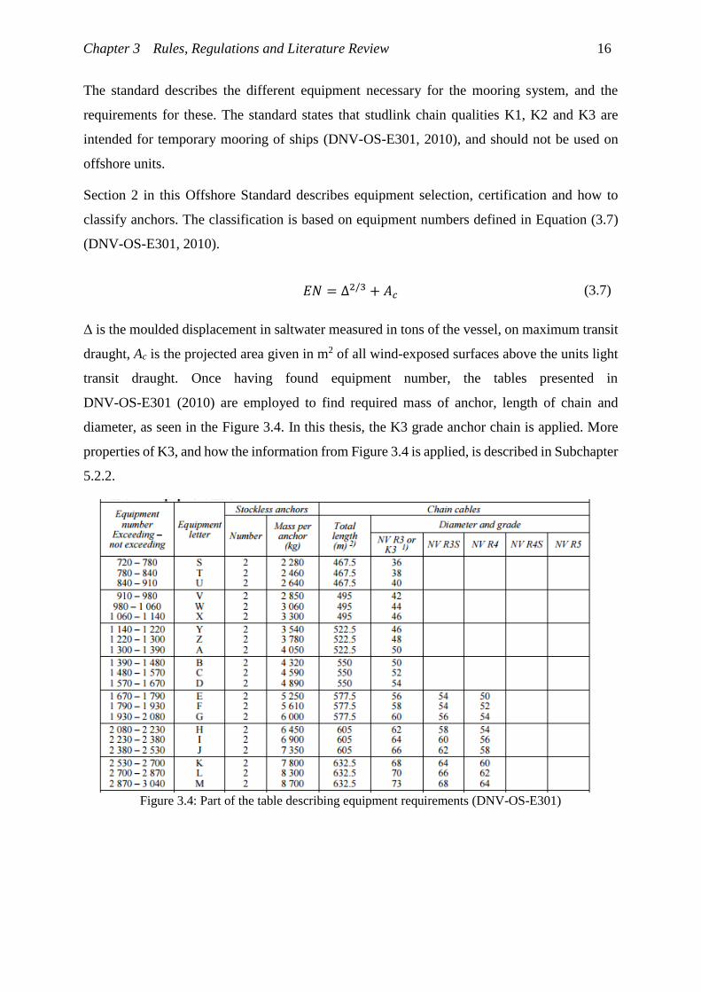
Section 2 in this Offshore Standard describes equipment selection, certification and how to
classify anchors. The classification is based on equipment numbers defined in Equation (3.7)
(DNV-OS-E301, 2010).
𝐸𝑁 = ∆2/3 + 𝐴𝑐 (3.7)
Δ is the moulded displacement in saltwater measured in tons of the vessel, on maximum transit
draught, Ac is the projected area given in m2 of all wind-exposed surfaces above the units light
transit draught. Once having found equipment number, the tables presented in
DNV-OS-E301 (2010) are employed to find required mass of anchor, length of chain and
diameter, as seen in the Figure 3.4. In this thesis, the K3 grade anchor chain is applied. More
properties of K3, and how the information from Figure 3.4 is applied, is described in Subchapter
5.2.2.
Figure 3.4: Part of the table describing equipment requirements (DNV-OS-E301)

Chapter 3 Rules, Regulations and Literature Review 17
3.1.3 DNV-RP-F111
Interference Between Trawl Gear and Pipelines (DNV-RP-F111, 2010) is the recommended
practice for calculating loads induced by trawl gear on pipelines. The interaction is described
as a two-stage situation. First, the anchor causes an impact on the pipeline, which is then
followed by either a pull over or a hooking. The recommended practice explains how to
calculate the impact force, the depth of the local dent and the energy absorbed by the pipeline.
For the pull over, it also illustrates how to calculate the pull over duration. For the hooking
situation, it simply states that the response during hooking should be found by applying relevant
and conservative models, without going into more detail.
It is clearly stated in the recommended practice that the loads and load effects found are related
to size, shape, velocity and mass of the trawling gear. The equations presented can therefore
not be directly applied to calculate anchor loads, but they can be used to calculate the
approximate impact force and denting caused on the pipelines.
As the loads and load effects are affected by size, shape, velocity and mass of the impacting
object, it is reasonable to assume that these parameters will have an effect on the
anchor-pipeline interaction.
3.2 Research Papers
Two research papers have particular relevance for the modelling and study of anchor-pipeline
interaction. The first one, Effect of Ship Anchor Impact in Offshore Pipeline (Al-Warthan et al.,
1993), investigates the dynamic pipeline response, within the elastic range, in the event of
anchor-pipeline interaction. The analysis is performed by using Discrete Element Method
(DEM). The paper’s main focus is on how the span length, that is the free span of the pipeline,
may affect the outcome of such a situation.
In the second one, Assessment of Anchor Dragging on Gas Pipelines (Sriskandarajah &
Wilkins, 2002), the authors assess the force needed to initiate lateral movement of a subsea
pipeline, force needed for the pipeline to reach its maximum allowable design stress and force
needed to cause local buckling. This is done for pipelines resting on the seabed, and buried, by
performing a dynamic non-linear FEA using ABAQUS.
Al-Warthan et al. (1993) model a 16-inch pipeline with rigid body elements connected with
lumped axial, shear and bending stiffness. Plastification and local buckling are excluded in the

Chapter 3 Rules, Regulations and Literature Review 18
study, as is environmental loading by applying a constant vessel velocity of 1 knot. The results
are found using time integration scheme with an updated Lagrangian approach. Sriskandarajah
and Wilkins (2002) on the other hand model a 10 km long pipeline using an element that enables
prediction of collapse buckling. The outer diameter is not listed.
Al-Warthan et al. (1993) define two different interaction modes: dropped anchor and hooking,
while Sriskandarajah and Wilkins (2002) define two phases of the interaction: initial impact
followed by dragging of the pipeline. The latter authors also establish drag embedment anchors
as the type of anchor most likely to cause a hooking event, as in the case with the Kvitebjørn
pipeline (Gjertveit et al., 2010). Al-Warthan et al. (1993) simplify the modelling of the
interaction by not modelling the anchor, but instead defining three load cases for an anchor of
4310 kg. The initial impact caused by a dropped anchor is modelled as an impulse load with
either a triangular impulse shape factor or a ramp loading. The basic expression for an impulse
is shown in Equation (3.8) (Al-Warthan et al., 1993).
𝐼𝐼 = ∫ 𝐹𝑑𝑡 = 𝑚𝑣2 −𝑚𝑣1
𝑡2
𝑡1
(3.8)
𝐼𝐼 = 𝑚𝑣0 = 𝐶𝐼𝐹𝑡𝑑 (3.9)
m is the anchor mass, v1 and v2 are the initial and final velocities respectively. The alternative
way of writing the equation, seen in Equation (3.9), employs the initial velocity of the anchor
v0, or the maximum impact load F, duration of impact td and the impulse shape factor CI. Hertz
theory is applied to find the duration of the impact, as seen in Equation (3.10). k1 is a function
dependent on the Young’s modulus, Poisson’s ratios and the mass for pipe and anchor.
𝑡𝑑 = 𝑘1𝑣0
−15 (3.10)
Al-Warthan et al. (1993) model the hooking load by use of catenary equations, and the
expression seen in Equation (3.11), to express the upward vertical tension applied to the
pipeline.

Chapter 3 Rules, Regulations and Literature Review 19
𝑇 = 𝑇𝑥 [1 + √sinh (𝑊𝑐
𝑥 − (𝑥𝑟 − 𝑥𝑡)
𝑇𝑥)2
] (3.11)
𝑥𝑟 =
𝑇𝑥𝑊𝑐tanh1 (
ℎ
𝐿) +
𝑥𝑡2
(3.12)
Tx is the horizontal tension, xt is the downstream excursion, Wc is the total chain and anchor
weight, L is the total chain length and h is the water depth. This approach finds the tension in
the cable and applies it to the pipeline as a load increasing with time, as the horizontal tension
increases due to towing.
The approach of calculating tension transmitted onto the pipeline from the vessel when the
mooring lines take on the form of a catenary, is supported by Sriskandarajah and Wilkins
(2002). Sriskandarajah and Wilkins (2002) also claim that the worst case scenario would be if
the mooring line does not contact the seabed, as the full force from the vessel motion would be
exerted onto the pipeline.
The article by Al-Warthan et al. (1993) applies the same basic concepts as in the Recommended
Practice DNV-RP-F111 (2010) to calculate the initial loads on the pipeline, but simplifies it by
ignoring all effects of size and shape of the anchor. Sriskandarajah and Wilkins (2002) also
applies a simplified approach by applying internal and external pressure, followed by a
prescribed lateral displacement of 50 meters at the hooking location. This displacement was
applied statically.
Al-Warthan et al. (1993) demonstrates that the stresses increase with decreasing span length,
and that the highest amount of stresses are caused when the pipeline is exposed to a ramp
impulse load. A ramp impulse load is a dropped anchor that remains on the pipe. The results
indicate that the bending stress is always higher than the axial stress, independently of span
length. The article concludes that stresses exceed yield stress for the pipeline grade API X-65,
which would result in local buckling and yielding, making the pipeline unable to operate.
Sriskandarajah and Wilkins (2002) show that for a pipeline resting on the seabed, results
indicate a lateral force of 73 kN is necessary to displace the pipeline 1 meter in lateral direction,
while 150 kN is necessary to reach the design stress limit. A force of 525 kN is necessary to
begin the onset of lateral buckling. For the buried pipe, a lateral force of 400 kN is necessary to

Chapter 3 Rules, Regulations and Literature Review 20
displace the pipeline 1 meter, indicating the effectiveness of burying pipelines. Local effects on
the pipeline are not considered in this text.
Neither of the research papers model the anchor when simulating the interaction. Instead,
impulse loads are applied to inspect initial impact, and catenary calculations and prescribed
lateral displacements applied to inspect hooking. The effect of size and shape of anchor are thus
excluded from the studies.
3.3 Master theses
3.3.1 “Pipeline Accidental Load Analysis”
Vervik’s MA-thesis (2011) is based on the anchor hooking incident at the Kvitebjørn Gas
Pipeline. The thesis’ main goal is to predict the most probable loads induced by anchors if
hooking occurs, investigating what type and size of anchors can cause hooking and the
probability of a vessel with such an anchor passing the Kvitebjørn gas pipeline.
Similarly to Assessment of Anchor Dragging on Gas Pipelines (Sriskandarajah & Wilkins,
2002) drag embedment anchors of different classes are inspected, specifically classes of the
Spek anchor. Following DNV-OS-E301 rules and applying Equation (3.7), the anchors are
divided into six classes based on their equipment number described in Subchapter 3.1.2, seen
in Table 3.1 below.
Table 3.1: Equipment letter and class in Vervik’s (2011) thesis
Equipment Letter Anchor Mass [kg]
Class 1 z - G 3780 – 6000
Class 2 G – L 6000 – 8300
Class 3 L – O 8300 – 9900
Class 4 O – X 9900 – 15400
Class 5 X – A* 15400 – 17800
Class 6 A* - E* 17800 – 23000
𝐷𝑚𝑎𝑥 =
2𝐿(1 − 𝑐𝑜𝑠𝛼)
𝑠𝑖𝑛𝛼 (3.13)
The Spek anchor’s geometry, seen in Figure 2.2, has a maximum angle of 40 degrees between
the shank and the fluke. This makes the anchor optimal for hooking. By use of Equation (3.13)
Vervik (2011) shows that due to its geometric dimensions, anchors smaller than 3780 kg will

Chapter 3 Rules, Regulations and Literature Review 21
not manage to hook onto a pipeline with a steel diameter of 30 inches. In Equation (3.13) Dmax
is the maximum pipe diameter the anchor can hook onto; L is the fluke’s length and 𝛼 is the
angle between the fluke and shank. For this reason anchors smaller than 3780 kg are excluded
in the following analyses.
For anchor hooking to occur, several key parameters are identified. These are vessel velocity,
anchor mass, pipe diameter, chain length versus water depth and chain breaking strength.
Inspecting the Norwegian Coastal Administration’s (NCA), Automatic Identification System
(AIS), reveals that in the period from March 2010 to March 2011 there were 237 out of 7160
ships which could cause hooking (Vervik, 2011). This analysis is carried out for all segments
of the Kvitebjørn pipeline, which rest at varying depths. The distribution of anchor classes for
these 237 vessels is shown in Figure 3.5.
Figure 3.5: Distribution of the 237 vessels which cause hooking, figure by Vervik (2011)
The pipeline section with the largest ship traffic in the vicinity is located at a water depth of
300 meters. Based on the geometry of the Kvitebjørn pipeline and applying Equation (3.13), it
is concluded that Spek anchors of type z, G, L, O, X, A* and E* can cause hooking. However,
by applying SIMLA and inspecting the drag forces on the anchor when towed, and a water
depth of 300 meters, it is determined that only anchors of type O or larger can cause hooking at
this depth. This is due to the force exerted on the anchor and chain when towed, as well as the
maximum allowable length of anchor chain.
To study the forces applied on the pipeline during hooking, a global analysis is performed in
SIMLA. A similar approach to that of Al-Warthan et al. (1993) and Sriskandarajah and Wilkins
(2002) is employed as the response of the pipeline is the focus. The anchor-pipeline interaction
Chapter 3 Rules, Regulations and Literature Review 22
is modelled using a linear spring between the pipeline node and the anchor chain node. The
resistance properties of the spring is mimicking a triangular impulse load where the maximum
force is equal to the maximum anchor chain breaking load. The chain itself is modelled as a
single beam element with low bending stiffness to represent the bending flexibility of the chain,
and an axial stiffness corresponding to the applied anchor chain diameter (Vervik, 2011). The
pipeline is modelled as full-length with elastoplastic material properties.
The largest displacements and strain in the pipeline occurred at 5 knots, and lower values at
higher velocities. The large displacements results in the response being dominated by plastic
bending and the development of large membrane forces.
3.3.2 “Anchor Loads on Pipelines”
Wei’s MA-thesis (2015) is a continuation of Vervik’s MA-thesis from 2011. The focus of the
thesis is on creating a SIMLA model to inspect parameters necessary for hooking, and the non-
linear effects of hooking. The data regarding relevant anchors from Vervik’s (2011) thesis is
utilized, and the anchors of type z, G, O and X are studied.
Two models are produced for SIMLA. The first models the pipeline as a 10 meter long rigid
body, similar to the modelling done by Al-Warthan et al. (1993), and attempts to determine
which parameters are necessary to cause hooking. The second model consists of a full-length
pipeline of 10 kilometers with elastoplastic material properties, similar to the modelling done
by Sriskandarajah and Wilkins (2002) and Vervik (2011). This model attempts to display the
actual response of the pipeline when allowing non-linear effects. Unlike the aforementioned
research papers and MA-thesis, Wei (2015) models the anchor as a 3D object. The anchor’s
geometry is simplified, but is modelled using SOTRAs Spek anchor’s dimensions as a basis.
Which specific values were used to model the different anchors is however not clear.
The parameters inspected in the short model are the diameter of the pipe, anchor mass, span
height and the angle of attack between anchor and pipeline. The values used for the different
variables are shown in Table 3.2. The measured parameter is the tension in the anchor chain.

Chapter 3 Rules, Regulations and Literature Review 23
Table 3.2: Parameters inspected by Wei (2015)
Anchor mass [kg] Pipe Diameter [m] Hooking Angle [ ̊ ] 𝐒𝐩𝐚𝐧 𝐇𝐞𝐢𝐠𝐡𝐭
𝐃𝐢𝐚𝐦𝐞𝐭𝐞𝐫 [−]
3780 0.4 90 0
6000 0.6 100 1
9900 0.8 110 2
15400 1.0 120 3
Using SIMLA, 512 simulations are performed. The results show that increasing anchor size,
and decreasing pipe dimensions, cause a higher probability of hooking. Furthermore, larger
span heights reduces the probability of hooking, because the anchor will twine and bounce off
the pipeline. This is a response not seen in the research papers as the anchor is modelled as a
load on the pipeline. Lower vessel speed increases the probability for hooking, as in accord
with Vervik’s (2011) results.
The long pipeline model introduces elastoplastic material, instead of elastic, to inspect the
pipeline’s bending moment. Four different simulation are performed. The first three simulations
with a pipe diameter of 0.4 meters, a hooking angle of 90 degrees and a span height of 1.2
meters. The anchor types z, O and X are assessed. For anchor types z and O, the force in the
cables connected to the anchors will exceed their capacity limit, resulting in the cable breaking.
For anchor X this does not occur, which results in the conclusion that the pipe will rupture.
However, in the final simulation, the pipe diameter was increased from 0.4 to 0.6 meters, and
showed that the cable would once more fail. In other words, it is more likely that the cable will
break than the pipeline rupturing.
There are some uncertainties regarding the modelling in SIMLA that make it difficult to
replicate the results. For instance, it is uncertain exactly how the anchor is modelled. It is
uncertain whether the anchor geometry is updated with anchor mass, or the anchor geometry
has been held constant. It is also unclear whether the cable geometry and properties are updated
when the anchor mass is altered, and which cable length is applied. Which values were used for
the pipe’s properties is also somewhat uncertain, and if these properties were updated when
altering pipe diameter. Furthermore, it is uncertain which drag coefficients were used for the
cable. Because of this, comparing results will be difficult.
Despite no DNV rules or regulations specifically assessing anchor-pipeline interaction, general
rules regarding subsea pipeline in DNV-OS-F101 apply, and the recommended practice for

Chapter 3 Rules, Regulations and Literature Review 24
calculating trawl loads can be applied to find an approximation of anchor loads. Al-Warthan et
al. (1993) showed a simplified approach to calculate anchor loads by excluding anchor size and
shape. The loads were modelled either as an impulse load, or as tension applied to hooking
location. Sriskandarajah and Wilkins (2002) describes a method to assess the probability of an
anchor being dropped, and models the hooking onto the pipeline by applying a prescribed lateral
displacement. Vervik (2011) applies the method by Sriskandarajah and Wilkins (2002) to
inspect the probability of anchor hooking on the Kvitebjørn gas pipeline, and models the
interaction in SIMLA by connecting a spring between the cable and hooking location.
Wei (2015) is the first of these to create a model of the anchor when inspecting which
parameters increase the probability of hooking. However, the many uncertainties regarding how
the results were obtained may provide difficulties when comparing results. Wei’s (2015) model
does however create the basis for the modelling of the anchor-pipeline interaction. This is
described in more detail in Chapter 5.
The results from the research papers and the MA-theses indicate detrimental effects, such as
local buckling (Sriskandarajah & Wilkins, 2002) (Al-Warthan et al., 1993) and rupturing (Wei,
2015), should hooking occur. The two research papers conclude with local buckling, but both
ignore the effects of anchor geometry, by not modelling the anchor. The results from this thesis
will be compared with the two research papers described, and the two MA-theses.

25
Chapter 4
4 Non-linear Finite Element Analysis
To analyse the interaction between anchor and pipeline in this thesis the computer software
SIMLA was applied. SIMLA is a specified software used to perform analyses on umbilical
structures, such as pipelines. The software was originally created by MARINTEK for Norsk
Hydro ASA, after a request made in 2000 (MARINTEK, 2012). Its original purpose was to
simulate the structural response of a pipe during laying, and visualize the results. In later years
the use was extended, and as it allows for both non-linear static and dynamic analysis, it is an
optimal tool for inspecting anchor-pipeline interaction. In this chapter, the basics behind a non-
linear analysis are described, with focus on the methods applied in SIMLA.
According to Belytschko, Liu, Moran, and Elkhodary (2014) a non-linear analysis consists of
four steps:
1) Development of a model
2) Formulation of the governing equations
3) Solution of the equations
4) Interpretation of the results.
Several non-linear effects need to be considered when inspecting the structural behaviour of
subsea pipelines. According to Sævik (2014), these are:
1) Large displacements
2) Non-linear pipe-soil interaction forces
3) Non-linear material behaviour
4) Non-linear hydrodynamic loading
5) Variable boundary conditions
6) Transient temperature and pressure loads due to variable fluid flow conditions

Chapter 4 Non-linear Finite Element Analysis 26
A linear Finite Element Method (FEM) analysis assumes that the displacements are small, and
the material linear elastic (Moan, 2003b). This is not the case for anchor-pipeline interaction,
as the pipe may be exposed to large displacements. The non-linear effects relevant for anchor-
pipeline interaction analysis are large displacement, non-linear pipe-soil interaction forces and
non-linear material behaviour.
4.1 Basics of Finite Element Method
FEM is a method to calculate the response of a structure. This is done by discretizing the
structure into elements and nodes, calculating the response for the individual nodes and
elements, assimilating the responses and applying boundary conditions before calculating the
global response (Moan, 2003a). The basic principles of FEM according to Moan (2003b) are:
1) Equilibrium, expressed by stresses
2) Kinematic compatibility, expressed by strains
3) Stress-strain relation
These principles will be inspected in more detail, with focus on how they are implemented in
SIMLA.
4.1.1 Equilibrium
The requirement of equilibrium demands that there is always equilibrium between external and
internal forces. This is enforced by applying the principle of virtual work, or the principle of
virtual displacement. The principle states that (Langen & Sigbjörnsson, 1986, p. 3.1):
The total virtual work performed by a system in equilibrium when it is subjected to
virtual compatible displacements is equal to zero.
This results in the equilibrium expression seen in Equation (4.1) (Sævik, 2014).
∫ (𝝈 − 𝝈𝟎): 𝛿𝝐𝑑𝑉 + ∫ 𝜌�̈� ∙ 𝛿𝒖𝑑𝑉 −
𝑉
∫ 𝒇 ∙ 𝛿𝒖𝑑𝑉𝑉
−∫ 𝒕 ∙ 𝛿𝒖𝑑𝑆 = 0𝑉𝑉
(4.1)
δu is the virtual displacement, 𝝈 is the natural stress tensor, 𝝈𝟎 is the initial stress tensor, 𝝐 is
the natural strain tensor, f is the related volume force vector and t is the traction on the volume
surface.
Chapter 4 Non-linear Finite Element Analysis 27
In Equation (4.1) natural stress and strain are applied, these refer to the deformed configurations
of the element. However, since non-linear effects are included, there is a need for a description
of stress and strain within the element that refers to the initial undeformed configurations. The
natural stress and strain are hence not preferred for non-linear analysis (Moan, 2003b). The
Green strain tensor E, and 2nd Piola-Kirchhoff stress tensor S refers to the undeformed
configurations (Sævik, 2014). These can therefore replace the natural strain and stress tensors
respectively. 2nd Piola-Kirchhoff is given by Equation (4.2) (Sævik, 2008).
𝑺 = 𝜌0𝜌𝑭−1 ∙ 𝝈 ∙ 𝑭 (4.2)
F is the deformation gradient, 𝝈 is the natural stress tensor, 𝜌 is the density of the deformed
configuration, and 𝜌0 is the density of the undeformed configuration. For strains smaller than
roughly 2%, the difference between 2nd Piola-Kirchhoff and the natural stress tensor will be
small, and hence are assumed equal.
4.1.2 Kinematic Compatibility
To obtain convergence of the solution for the finite element analysis, when reducing mesh size,
the element must be complete and compatible (Belytschko et al., 2014). Complete means that
the displacement function must be able to represent all rigid body modes and constant strain
modes (Moan, 2003a). Compatibility means that there is continuity over the element boundaries
and at the nodes, that is: there are no gaps or overlaps in the deformed body (Belytschko et al.,
2014). This principle dictates the appearance of the element’s shape or displacement functions.
In SIMLA it is assumed that Bernoulli-Euler and Navier’s hypothesis apply for the pipe
elements and that strain is expressed by Green strain tensor E. As the pipelines response will
be both elastic and plastic, it is assumed that the elements are classified as elastoplastic, which
is discussed in more detail in the following Subchapter 4.1.3. The displacements and
longitudinal Green strain which replaces the natural strain tensor in Equation (4.1) is expressed
in equation (4.3) (Sævik, 2008).
𝐸𝑥𝑥 = 𝑢𝑥0,𝑥 − 𝑦𝑢𝑦0,𝑥𝑥 − 𝑧𝑢𝑧0,𝑥𝑥 +1
2(𝑢𝑦0,𝑥
2 + 𝑢𝑧0,𝑥2 ) + 𝜃,𝑥(𝑦𝑢𝑧0,𝑥 − 𝑧𝑢𝑦𝑜,𝑥) +
1
2𝜃,𝑥2(𝑦2 + 𝑧2) (4.3)

Chapter 4 Non-linear Finite Element Analysis 28
𝑢𝑥(𝑥, 𝑦, 𝑧) = 𝑢𝑥0 − 𝑦𝑥𝑦0,𝑥 − 𝑧𝑢𝑧0,𝑥 (4.4)
𝑢𝑦(𝑥, 𝑦, 𝑧) = 𝑢𝑦0 − 𝑧𝜃𝑥 (4.5)
𝑢𝑧(𝑥, 𝑦, 𝑧) = 𝑢𝑧0 − 𝑦𝜃𝑥 (4.6)
4.1.3 Constitutive Equations
The constitutive equations explain the relation between stress and strain. For a linear elastic
material, Hooke’s law describes this relation, but for a plastic material, the situation becomes
more complicated due to plastic effects. The expression for total strain is seen in Equation (4.7)
(Sævik, 2014).
𝑬 = 𝑬𝑒 + 𝑬𝑝 (4.7)
Ee is the elastic strain expressed by elastic material law, and Ep is the plastic strain. Plastic strain
is the strain which results in permanent deformation. The relation between these is seen in the
stress-strain graph in Figure 4.1, where strain is denoted 𝜖.
Figure 4.1: Stress-strain showing elastic and plastic strain contribution (Moan, 2003b)
Chapter 4 Non-linear Finite Element Analysis 29
To find the plastic strain one needs to define (Moan, 2003b):
1) A yield criterion
2) A hardening rule
3) A flow rule
The yield criterion defines when the material is plastic and which combinations of multi-axial
stresses are necessary to move in plasticity. The flow rule describes the plastic strain
increments, while the hardening rule defines how the yield condition changes as plastic flow
proceeds (Sævik, 2008). These will now be described in more detail.
The yield criterion defines at which stress level plastic deformation first occurs, and is described
by Equation (4.8) (Sævik, 2008).
𝑓(𝑺, 𝜅) = 0 (4.8)
Where the equation describes a scalar function of S and 𝜅, which are the stress tensor of 2nd
Piola-Kirchhoff stress, and a strain-hardening parameter dependent on the history of the loading
in the plastic range. It is assumed that the yield surface is a closed surface, and the equation
above expresses this in the six-dimensional stress space (Sævik, 2008). A consistency condition
is necessary to describe that stress points remain on the yield surface during loading in the
plastic range. The consistency condition is given by Equation (4.9) (Sævik, 2008).
𝑓̇ =
𝜕𝑓
𝜕𝑺: �̇� +
𝜕𝑓
𝜕𝜅�̇� (4.9)
The hardening rule is necessary to describe how the yield criterion changes with the onset of
plastic deformation. In SIMLA both kinematic and isotropic hardening are included in the
material model (Sævik, 2008). Kinematic hardening means that one assumes that the yield point
and the effects of work hardening are the same in tension and compression (Moan, 2003b). This
is unlike isotropic hardening, where the material remembers the hardening, and requires an
unloading which is equal to twice the stress prior to unloading (Sævik, 2008). Isotropic
hardening also means that yield surface expands isotropically, while staying centred at origin
(Kyriakides & Corona, 2007). Kinematic and isotropic hardening are seen in Figure 4.2.

Chapter 4 Non-linear Finite Element Analysis 30
Figure 4.2: Kinematic and isotropic hardening (Moan, 2003b)
As metal plasticity is path dependent, the flow rule is needed to express the relation between
the strain increments to the stress increments. The flow rule is based on Drucker’s postulate
that (Kyriakides & Corona, 2007):
1) Yield-surfaces are convex,
2) The instantaneous plastic strain increment at σ is normal to the yield surface,
3) The strain increments are linearly related to the stress increments.
4.2 Co-rotational Total Lagrangian Formulation
When describing non-linear problems the choice of reference system needs to be carefully
considered. In SIMLA a Co-rotated Total Lagrangian system is applied (Sævik, 2008). A
Lagrangian description of the motion uses the material particle as a reference point (Moan,
2003b). There are two main types of Lagrangian formulation: Total and Updated. The basic
idea behind these two formulations is to separate rigid body motions from the local deformation
of the element (Sævik, 2008). The difference between the two formulations is that total
Lagrangian is based on a fixed coordinate system, where all deformations refer to the initial
configuration (Moan, 2003b), while updated Lagrangian operates with a local coordinate
system that has to be updated when the geometry changes due to deformations (Sævik, 2008).
Deformations in the latter formulation do not refer to the initial configuration, but rather the
previous configuration.
The Co-rotational formulation is a combination of the two described above. All quantities refer
back to the initial configuration, but there is a local coordinate system attached to the element

Chapter 4 Non-linear Finite Element Analysis 31
that is allowed to both translate and rotate with the element (Sævik, 2008). The Co-rotated
system then employs four base vector systems. The first one is a fixed global system with axis
Xi and base vectors Ii, where i is the directions 1, 2 or 3. The second is a local coordinate system
attached to each node of the element and continuously updated to capture the rotations at the
nodes. This system is defined with axis xi and base vectors ii. The third one is an element end
coordinate system that defines how the different elements connected to the node are oriented
relative to the nodal coordinate system. This system is only defined once and not updated. The
last one is a local element system at each element used to find the element deformations with
coordinate axes yi and base vectors ji (Sævik, 2008). The large displacements are accounted for
by continuously updating the element and node orientation, as well as the position of the end
coordinates. In Figure 4.3 the global coordinate system is seen at the top, with a node centred
between three elements below. In this node one can see the nodal coordinate system base
vectors (i) and the element end base vectors (j).
Figure 4.3: Global (I), nodal (i) and element base (j) vector (Sævik, 2008)
The incremental equilibrium expressed by Equation (4.10) below is used as the basis for the
stiffness matrix. This equations is found from Equation (4.1), by applying the Co-rotational
Total Lagrangian formulation and the basics of the FEM described in Subchapter 4.1, while
neglecting higher order terms and assuming that the difference between two neighbouring
equilibrium states are small (Sævik, 2008).

Chapter 4 Non-linear Finite Element Analysis 32
∫ 𝑪: ∆휀: 𝛿휀𝑑𝑉0 +𝑉
∫ 𝝈: 𝛿∆𝑬𝑑𝑉0 −𝑉
∫ ∆𝒕𝑑𝑆0 = 0𝑆
(4.10)
C is the elasticity tensor, S is the 2nd Piola-Kirchhoff, E is the Green strain tensor, 𝛿 is the
virtual quantity, ∆ is the increment between two configurations, t is the referential surface
traction vector and 𝝈 is the Cauchy stress tensor. The first term describes the material stiffness,
while the second term describes the geometric stiffness matrix. The material stiffness reflects
the alteration of the stiffness caused by change in geometry due to deformation, while the
geometric stiffness is the stiffness caused by initial member forces prior to displacement (Moan,
2003b).
4.3 Solution Methods
As the anchor’s impact on the pipeline is a dynamic load dependent on time, a dynamic analysis
has to be performed. Before this, a static analysis has to be performed to ensure that the system
is in equilibrium before the onset of the dynamic load. The main difference between dynamic
loads and static loads are (Langen & Sigbjörnsson, 1986, p. 1.2):
1) Dynamic loads imply a time dependent solution
2) Dynamic loads introduce inertia loads throughout the structure
Since large deformations are allowed and non-linearities are included, an incremental approach
has to be implemented to find the static and the dynamic solution.
4.3.1 Static Solution
The expression for the static problem is seen in Equation (4.11).
𝑲𝒓 = 𝑹 (4.11)
K is the stiffness, R is the applied force, and r is the displacement. In Equation (4.11) the
stiffness K is the total global stiffness consisting of all contributions to the stiffness, that is the
material or initial stress stiffness and the geometric stiffness seen in Equation (4.10). The
contributions are summed together, and transformed from a local to a global matrix using a
transformation matrix. The global stiffness matrix is then created by summing together the

Chapter 4 Non-linear Finite Element Analysis 33
contributions. The solution of Equation (4.11) is found by use of user defined load control, with
Newton-Raphson equilibrium iteration at each load step (Sævik, 2008). The equation can then
be rewritten to incremental form, as seen in Equation (4.12), and solved by applying Equation
(4.13) and (4.14) (Moan, 2003b).
∆𝒓𝑘+1𝒊 = 𝑲𝑇,𝑘+1
−𝟏𝒊 ∙ ∆𝑹𝑘+1𝒊 (4.12)
𝒓𝑘+1 − 𝒓𝑘 = ∆𝒓𝑘+1 = 𝑲𝐼−1(𝒓𝑘)(𝑹 − 𝑹𝒊𝒏𝒕) (4.13)
𝒓𝑘+1 = 𝒓𝑘 + ∆𝒓𝑘+1 (4.14)
This requires an update of the stiffness matrix for each load step. To reduce computational
power, modified Newton-Raphson may be applied, here the stiffness matrix is not updated for
each load step. The modified Newton-Raphson iteration is seen in Figure 4.4 below.
Figure 4.4: Modified Newton-Raphson iterations (Moan, 2003b)
4.3.2 Dynamic Solution
The expression for the dynamic equation of motion is seen in Equation (4.15).
𝑴�̈� + 𝑪�̇� + 𝑲𝒓 = 𝑸 (4.15)
M denotes the mass matrix, C is the damping matrix, K is the stiffness matrix, Q is the load
vector and r is the displacement vector. When non-linear effects are included this equation can
be solved by applying modal superposition. This means that the dynamic equation of motion is

Chapter 4 Non-linear Finite Element Analysis 34
expressed as a number of uncoupled equations which may be solved by direct time integration
(Moan, 2003b).
The solution to Equation (4.15) can either be found by explicit or implicit methods. The explicit
methods use only current and previous time step results to find the results for the next time step.
Explicit solution methods are conditionally stable as long as the time steps are small enough,
which makes the method appropriate for explosion and impact analysis (Sævik, 2008). If
however the analysis requires a long duration, it is more appropriate to apply implicit methods.
The expression for an implicit method is seen in Equation (4.16).
𝒓𝑘+1 = 𝑓(�̈�𝑘+1, �̇�𝑘+1, �̈�𝑘, �̇�𝑘, 𝒓𝑘, … ) (4.16)
These methods will generally have a better numerical stability. Very small time steps will
however make this method uneconomical with regards to computational effort and time. For
the anchor-pipeline interaction simulation in SIMLA, implicit methods are applied, along with
the incremental time integration scheme HHT-α.
The reason for applying this specific scheme is that the lower modes are the most interesting
for the response. It is hence desirable to avoid higher and medium modes (Langen &
Sigbjörnsson, 1986). If Rayleigh-damping is introduced in the Newmark-β scheme, the medium
modes are damped out. Applying Newmark-β will however result in reduced accuracy. This
can be counteracted by introducing the HHT-α scheme. Without going into too much detail,
HHT-α becomes Newmark-β when α is equal to zero. The HHT-α scheme results in accuracy
remaining, while damping out the higher frequencies. The modified equilibrium equation of the
system is seen in Equation (4.17) (Moan, 2003b).
𝑴�̈�𝑘+1 + (1 + 𝛼)𝑪�̇�𝑘+1 − 𝛼𝑪�̇�𝑘 + (1 + 𝛼)𝑹𝑘+1𝐼 − 𝛼𝑹𝑘
𝐼
= (1 + 𝛼)𝑹𝑘+1𝐸 − 𝛼𝑹𝑘
𝐸 (4.17)
Where M is the mass matrix, RI is the internal force, RE is the external force, and C is the
damping matrix consisting of both diagonal damping terms and Rayleigh-damping described
by Equation (4.18).
𝑪 = 𝑪0 + 𝛼1𝑴+ 𝛼2𝑲 (4.18)

Chapter 4 Non-linear Finite Element Analysis 35
C0 is the diagonal damping matrix, while the two other terms are the Rayleigh-damping where
α1 is the mass proportional damping factor and α2 is the stiffness proportional damping factor.
Equation (4.17) will be unbalanced, and hence, requires equilibrium iterations. The updated
Newton-Raphson approach described in Subchapter 4.3.1 is one possible approach to perform
these iterations.


37
Chapter 5
5 Modelling
The purpose of this chapter is to describe the modelling of the anchor-pipeline interaction. To
model the interaction, the anchor, chain and pipeline must be modelled. In addition, the seabed,
sea surface and environmental conditions have to be specified. All of the necessary components
needed to create the model are seen in Figure 5.1, with the applied coordinate system. The
anchor moves in negative Y-direction, the X-axis points into the plane and Z is zero at the sea
surface.
Figure 5.1: All components needed to model the interaction, with coordinate system
A total of three separate analyses were carried out to inspect the anchor-pipeline interaction.
The first analysis investigated the effect of anchor mass, anchor geometry, pipe diameter, vessel
velocity and angle of attack on the anchor’s response. The angle of attack was defined as seen
in Figure 5.2. The second analysis determined minimum chain length for the anchors to reach
the seabed when towed at 2 and 10 knots. The final analysis consisted of eleven case studies,
which investigate the global response of the pipeline when exposed to anchor forces. The
collective term for the eleven cases are elastoplastic case studies.

Chapter 5 Modelling 38
Figure 5.2: Angle of attack between pipeline and anchor
For all of the analyses, the water depth was 200 meters. The pipe was assumed to be grade
X-65. All objects made of steel were assumed to have the same general material properties.
These and other general properties applied in the analyses are shown in Figure 5.1. The naming
system seen in Figure 5.3 was used for the parametric study, and the case studies, to easily
distinguish the models. Figure 5.4 displays the naming system used for the study of minimum
required chain length.
Table 5.1: General properties applied in the analyses
Symbol Value Unit
Young’s Modulus E 2.10∙1011 Pa
Shear Modulus G 7.93∙1010 Pa
Gravitational acceleration g 9.81 m/s2
Density seawater 𝜌𝑠𝑒𝑎𝑤𝑎𝑡𝑒𝑟 1026 kg/m3
Density steel 𝜌𝑠𝑡𝑒𝑒𝑙 7850 kg/m3
Water Depth 𝑏 200 m
a – Anchor Mass [kg]
b – Water depth [m]
c – Pipe diameter [in]
d – Vessel velocity [kn]
e – Chain length [m]
f – Angle of attack [ ̊ ]
𝒂kg𝒃m𝒄in𝒅kn𝒆m𝒇
Example: 𝟒𝟖𝟗𝟎kg𝟐𝟎𝟎m𝟑𝟎in𝟐kn𝟓𝟓𝟎m𝟗𝟎
Figure 5.3: Naming system

Chapter 5 Modelling 39
a – Anchor Mass [kg]
d – Vessel velocity [kn]
e – Chain length [m]
𝒂kg𝒅kn𝒆m
Example: 𝟒𝟖𝟗𝟎kg𝟐kn𝟓𝟓𝟎m
Figure 5.4: Naming system for required anchor chain length
All the time-domain analyses were carried out by applying MARINTEK’s special purpose
computer tool SIMLA. The next subchapter will give an overview over SIMLA’s structure, and
how a SIMLA analysis is performed. Following this, the elements in SIMLA, and how they
were applied to model the components seen in Figure 5.1 is described. This includes
simplification of geometry and calculations performed using MATLAB. Finally, the analyses’
setup is described.
5.1 SIMLA
To perform a SIMLA analysis several modules are employed, as seen in Figure 5.5. Models are
created using FlexEdit, which is a text editor consisting of ASCII characters and based on cards
that define specific aspects of the model (Sævik, Økland, Baarholm, & Gjøsteen, 2010).
FlexEdit creates a .sif file that is run by SIMLA which produces the output file .sof, the log file
.slf, as well as the results database .raf and .dyn. The .raf file is used by XPost to create a 3D
visualization. To create plots of the responses, a .spi file is made specifying which responses
are to be inspected. SIMPOST takes this .spi file and creates a .mpf file consisting of ASCII
characters which can be utilized by MatrixPlot to create plots.

Chapter 5 Modelling 40
Figure 5.5: Overview over modules from SIMLAs user manual (Sævik et al., 2010)
When creating the model using FlexEdit, one first defines nodal coordinates before attaching
elements to these nodes (Sævik, 2008). These elements are organized into element groups,
which are given a chosen name and defined by the choice of element and material type. In the
modelling of the anchor-pipeline interaction, four different element types were applied. These
are PIPE31, PIPE33, CONT126 and CONT164. The first two are pipe elements, used to model
the anchor, pipeline and cable. The two latter elements are contact elements applied to model
the interaction between the pipe elements and the seabed, and between the pipe elements. These
elements will be reviewed.
5.2 Pipe Elements
Pipe elements are 3D elements modelled with two nodes. They are employed to model all
physical objects in the models, that is the anchor, anchor chain and pipeline. By default it is
assumed that the pipe elements have thin walled tubular cross-sections with constant radius and
constant thickness along each element (Sævik, 2008). This can however be bypassed by
applying the card NODPROP.
For the pipe elements, the mass matrix is found by applying interpolation functions that assume
six degrees of freedom per node; three translational and three rotational degrees of freedom
(Sævik, 2008). Raleigh and lumped damping is included for each element. Loads applied to
the elements include linear interpolations loads along the element, and hydrodynamic loads

Chapter 5 Modelling 41
found using Morison’s equation (Sævik, 2008). Both pipe elements apply the Co-rotational
Total Lagrangian approach, described in Chapter 4.2.
The defining difference between PIPE31 and PIPE33 is the material models and the kinematic
representation. PIPE31 assumes an elastic linear material, with plane stress and applies Hooke’s
law, resulting in two normal stress components and one shear stress component.
PIPE33 is an elastoplastic material that takes into consideration both stresses in axial and hoop
direction. The plastic properties of the element follows the outline described in Chapter 4.1.3.
The Green strain tensor expressed in Equation (4.3) is valid for PIPE33 elements. However, for
the elastic element PIPE31, the coupling between longitudinal strain and torsion is neglected
and the Green strain is shortened to the expression seen in Equation (5.1).
𝐸𝑥𝑥 = 𝑢𝑥0,𝑥 − 𝑦𝑢𝑦0,𝑥𝑥 − 𝑧𝑢𝑧0,𝑥𝑥 +1
2(𝑢𝑦0,𝑥2 + 𝑢𝑧0,𝑥
2 ) (5.1)
5.2.1 Anchor
In accord with prior work done by Vervik (2011) and Wei (2015), and as described in
Chapter 2.2, a stockless SOTRA Spek anchor was applied.
The information required to model the anchor and chain were stored in the excel spreadsheet
Input Anchor, seen in Appendix F. The anchor shape was simplified to the shape seen in Figure
5.6, and it was assumed that the mass was equally distributed.
Figure 5.6: Simplified geometry seen above and from the side

Chapter 5 Modelling 42
Important nodes have been listed with numbers in Figure 5.6, while dimensions taken from
SOTRA, seen in Table 2.1, are shown as bolded letters in accord with SOTRAs notation. Node
40011 has a vertical distance from the seabed of 0.2 meters. To model different anchors, the
coordinates implemented in the .sif file had to be updated. This was done using the MATLAB
script CoorAnchor.m that calculates the nodal coordinates for the anchor. The calculation of
the coordinates and distributed mass, is seen in the anchor section of Appendix C. The
MATLAB script is seen in Appendix F.
The anchor was modelled using PIPE31 elements, as deformation of the anchor should be small
and are hence unimportant. The anchor geometry was split into three parts. The fluke split into
two separate parts, and the shank modelled as one piece. The flukes have a varying radius at
each node, creating a pointed end at the tips, as can be seen the anchor modelled in Figure 5.7.
Should the anchor appear to deform, an option was to stiffen the anchor by adding three new
elements, one along each fluke and one along the shank. These elements have no mass or
geometric properties, but have a bending stiffness a hundred times stiffer than the original
bending stiffness. This approach can be applied to prevent the deformation of the anchor’s
flukes. This approach was applied in all of the elastoplastic case studies, but not in the
parametric study. This is discussed in more detail in Subchapter 6.1.2.
Figure 5.7: Anchor modelled seen in XPost

Chapter 5 Modelling 43
5.2.2 Chain
As mentioned in Chapter 3.1.2, K3 studlink chain was applied. SOTRA recommends a larger
diameter for the chain than DNV requires. In this thesis, DNV’s requirements were applied.
This means that the mass of the anchor dictates the diameter of the K3 chain found in DNV-
OS-E301 (2010), which in return dictates the break load and approximate mass of chain, found
in Table E2 in DNV Rules for Classification of Ships (2011). This information was also
included in the excel spreadsheet Input Anchor, seen in Appendix F. From the same set of rules,
the drag coefficients for studlink chains were found to be 2.6 in transverse direction, and 1.4
longitudinal.
When modelled the chain geometry, the shape was simplified to a circular section with a total
diameter equal to four times the diameter given for one link’s circular cross-section seen in
Figure 2.3 as D. The axial, bending and torsional stiffness were calculated by use of MATLAB
script CoorCable.m. To allow flexibility in the chain, the cross-sectional area of one chain
segment was found by multiplying the cross-sectional diameter of one link two.
The chain was modelled with 1000 PIPE31 elements. In the parametric study and the case
studies these 1000 elements were divided into three segments. The first segment was the one
attached to the anchor. The elements here were the same length as one chain link, that is:
𝑙𝑒𝑙𝑒𝑚𝑒𝑛𝑡 = 6 ∙ 𝐷𝑐ℎ𝑎𝑖𝑛 [𝑚] (5.2)
The next two segments consisted of the remaining elements. The second segment contained
two-thirds of the elements, and the last segment one-third. In the models, the chain was
separated into two element groups. This was to enable the possibility of making the top elements
stiffer than the others. However, this was not used and will not be described further. In the
required anchor chain length study the 1000 elements were modelled equally long.
The calculations performed in the MATLAB scripts to determine the properties of the chain,
size of chain elements and chain coordinates, can be seen in Appendix C, while the scripts are
seen in Appendix F.
5.2.3 Pipeline
To create a realistic model of the pipeline, certain assumptions were made regarding material
of the coating and content. These are seen in Table 5.2. As mentioned earlier it was assumed
that the pipeline was of grade X-65, in accord with Vervik (2011), and that the given parameters

Chapter 5 Modelling 44
from Statoil were the outer steel pipe diameter. The total outer diameter for the 30- and 40-inch
pipeline with protective coating are seen in Table 5.2.
Table 5.2: Important pipeline parameters
Property Value Unit
Density steel 7850 𝑘𝑔/𝑚3
Density asphalt 1300 𝑘𝑔/𝑚3 Density concrete 2500 𝑘𝑔/𝑚3 Density content 800 𝑘𝑔/𝑚3
Thickness asphalt layer 6 mm
Thickness concrete layer 45 mm
Total outer diameter (30-inch) 864 mm
Total outer diameter (40-inch) 1118 mm
The distributed weight of the pipe, as well as submerged weight, was calculated by use of
MATLAB function PipeMass.m seen in Appendix F. The calculations are summarized in
Appendix C.
As the main purpose of the parametric study was to investigate the anchor’s behaviour, PIPE31
elements were chosen for the pipeline. The pipe was modelled as a 10 meter long rigid body,
using two elements constrained against all displacements. When inspecting the actual response
of the pipeline in the eleven case studies, PIPE33 elements were chosen for modelling of the
pipeline. This was to create a more realistic response where the pipeline was modelled with
elastoplastic material. The pipeline was modelled as 10 kilometer long, only constrained at the
end nodes, allowing displacements otherwise. The pipeline was not modelled in the minimum
chain length study.
5.3 Contact elements
Contact elements calculate the gap between a prescribed master group and a slave group. If the
gap is sufficiently small to ensure contact, the elements will calculate the force between the two
contacting elements. The force is based on relative velocity and prescribed stiffness found from
the material curves (Sævik, 2008).
In the analyses, two contact element types were applied. The CONT126 element type was
applied to model general interaction between the physical objects and the seabed, where the
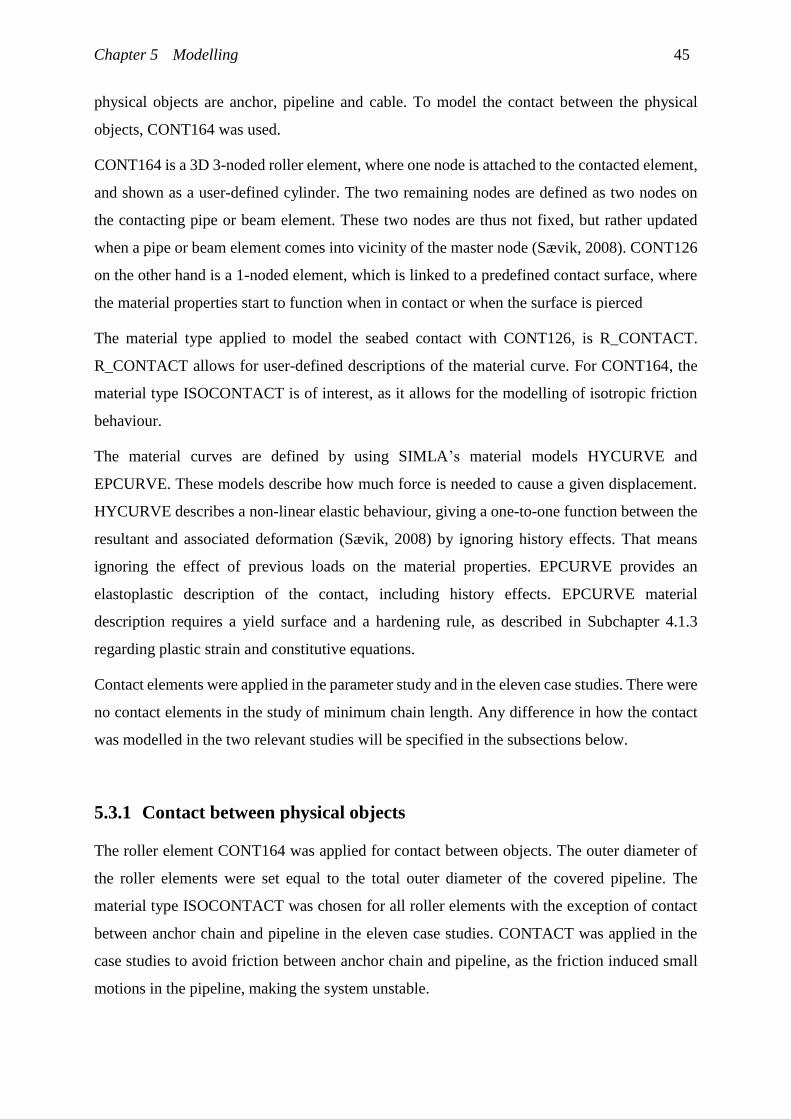
Chapter 5 Modelling 45
physical objects are anchor, pipeline and cable. To model the contact between the physical
objects, CONT164 was used.
CONT164 is a 3D 3-noded roller element, where one node is attached to the contacted element,
and shown as a user-defined cylinder. The two remaining nodes are defined as two nodes on
the contacting pipe or beam element. These two nodes are thus not fixed, but rather updated
when a pipe or beam element comes into vicinity of the master node (Sævik, 2008). CONT126
on the other hand is a 1-noded element, which is linked to a predefined contact surface, where
the material properties start to function when in contact or when the surface is pierced
The material type applied to model the seabed contact with CONT126, is R_CONTACT.
R_CONTACT allows for user-defined descriptions of the material curve. For CONT164, the
material type ISOCONTACT is of interest, as it allows for the modelling of isotropic friction
behaviour.
The material curves are defined by using SIMLA’s material models HYCURVE and
EPCURVE. These models describe how much force is needed to cause a given displacement.
HYCURVE describes a non-linear elastic behaviour, giving a one-to-one function between the
resultant and associated deformation (Sævik, 2008) by ignoring history effects. That means
ignoring the effect of previous loads on the material properties. EPCURVE provides an
elastoplastic description of the contact, including history effects. EPCURVE material
description requires a yield surface and a hardening rule, as described in Subchapter 4.1.3
regarding plastic strain and constitutive equations.
Contact elements were applied in the parameter study and in the eleven case studies. There were
no contact elements in the study of minimum chain length. Any difference in how the contact
was modelled in the two relevant studies will be specified in the subsections below.
5.3.1 Contact between physical objects
The roller element CONT164 was applied for contact between objects. The outer diameter of
the roller elements were set equal to the total outer diameter of the covered pipeline. The
material type ISOCONTACT was chosen for all roller elements with the exception of contact
between anchor chain and pipeline in the eleven case studies. CONTACT was applied in the
case studies to avoid friction between anchor chain and pipeline, as the friction induced small
motions in the pipeline, making the system unstable.

Chapter 5 Modelling 46
ISOCONTACT was chosen for all roller elements, with the exception mentioned above, to
include friction when inspecting impact and sliding. The friction coefficient in local XY-
direction for the anchor was defined as 0.50, and as 0.38 for the anchor chain, as recommended
by supervisor Prof. Sævik. To ensure that the anchor would not penetrate the pipeline, the
material curves of the roller elements, connected to the pipeline, were made sufficiently stiff.
For the parametric study, three CONT164 roller elements were created to model the contact
between the anchor segments and the pipeline, and one roller group was created to model the
contact between chain and pipeline. All of these element groups were attached to one of the
pipe elements and was roughly 100 meters long. This was to allow the anchor to slide along the
pipeline.
In the elastoplastic cases studied, the same approach as above was applied when the angle of
attack was 90 degrees, with the exception of case 15400kg200m30in2kn660m90 due to
erroneous results. For this case, and the cases where the angle of attack was 60 or 30 degrees,
the total number of roller elements were increased to 28. One element was for contact with the
cable, and was 20 meters long, connected to the element where the anchor would hit the
pipeline. The remaining 27 elements were divided into three groups of nine elements each. One
group for each fluke, and one for the shank. These elements were eleven meters long, and
overlapped with one meter, so that the anchor would be able to slide along the pipeline.
5.3.2 Contact with seabed
In the models created for the parametric study and the elastoplastic case studies, six contact
element groups were created to model interaction with the seabed. One contact element for each
of the three segments of the anchor, two for the cable and one for the pipeline. All of these
element groups share the same properties in regards to friction coefficients. The friction
coefficient in X-direction was set to 1.0, and in Y-direction to 0.3. However, the anchor chain
and the seabed contact element was rotated by 90 degrees. This means that the cables friction
coefficient in X-direction works in Y-direction, and the friction in Y-direction is valid for
motion in X-direction. The friction coefficient for the anchor when moving along the Y-axis
towards the pipeline would be 0.3, while the friction coefficient would be 1.0 for the cable. The
reason for doing this was DNV’s recommendation to use a friction coefficient of 1.0 between
chain and sea bottom (DNV-OS-E301, 2010). For the analyses where sliding was a possible

Chapter 5 Modelling 47
response, the friction coefficient in X-direction was altered from 1.0 to 0.3 when allowing
sliding. This is to ensure correct friction coefficient when the anchor slides.
The cable was also exposed to damping from the seabed due to soil material. To create this
effect damping was also included. The calculation for damping is seen in Equation (C-19) to
(C-21) in Appendix C.
The material curves used for soil stiffness were taken directly from Wei (2015), and have not
been altered. Hence, the soil stiffness was stiffer than it should be in the case of normal clay,
meaning that the anchor and pipeline do not penetrate the seabed as much as they should. Due
to time limitations, the material curves were not inspected in detail, and the material modelling
was not updated. This is however not a problem, as the largest effect of the soil stiffness, on the
interaction, is where the anchor hits the pipeline. That is, if the anchor penetrates the soil
considerably, it will have a different attack point on the pipe, than if it doesn’t penetrate the
soil. This effect can be produced by altering the span height of the pipeline. This was however
outside the scope of this thesis.
5.4 Environmental conditions and other parameters
The environmental conditions need to be defined for all of the analyses. However, they do not
have any effect on the simulation as the vessels movement was modelled as a constant velocity
applied at the top of the anchor chain. The motion of the vessel was thus modelled by applying
a PDISP card on the top of the cable. This card defines a factor, which is multiplied with a time
history, to calculate the displacement of the top of the anchor chain. The factor is dependent on
the chosen vessel velocity. Two different time histories were defined for the two velocities.
This was to prevent a too rapid acceleration of the 10 knot scenario, which could cause an
unrealistically large force in the anchor chain. Additionally, the top of the anchor chain had to
be moved backwards towards the anchor to create a catenary shape before the onset of motion.
This was to avoid large tension in the chain. To ensure this, the time histories were modified so
that the anchor chain would achieve a catenary shape, and the acceleration of the chain would
increase linearly until reaching desired velocity. The catenary shape was not necessary for the
required anchor length study as the chain started in a vertical position.
Other parameters that needed to be modelled was the angle of attack between anchor and
pipeline. In the parametric study this was done by applying a PDISP card to rotate the pipeline

Chapter 5 Modelling 48
elements. The rotation was performed during the second static analysis. For the elastoplastic
case studies, the coordinates for the pipeline after rotation were calculated and applied.
5.5 Specifics of Analyses
5.5.1 Parametric study
Model Setup
All components seen in Figure 5.1 were included in the parametric study, and modelled as
described above. The pipe was modelled using PIPE31 elements, extra stiffness was not applied
to the anchor, and the contact between physical objects was modelled with four roller elements.
The parameters studied were pipe diameter, anchor mass and geometry, vessel speed and angle
of attack between pipe and anchor. The chain length was set to the maximum value
corresponding to requirements in DNV-OS-E301 (2010) set by anchor mass, see Figure 3.4.
Six anchor classes were chosen to be applied in the parametric study, based on the study by
Vervik (2011). Parameters investigated are summarized in Table 5.3. The anchor chain length
in Table 5.3 is the maximum anchor chain length recommended by DNV for the anchor mass
listed to the left in the table.
Table 5.3: Parameters investigated
Anchor
Mass [kg]
Anchor
Class
Pipe Diameter
[Inches]
Vessel velocity
[knots]
Anchor Chain
Length [m]
Angle of
Attack [deg]
3780 Z 30 2 522.5 90
4890 D 40 10 550 60
6000 G 577.5 30
7800 K 632.5
9900 O 660
15400 X 742.5
The anchors starting point, relative to the pipelines, was determined based on chain length. The
longer the chain, the further away it would start. To investigate all combinations of the
parameters, 72 analyses were carried out.

Chapter 5 Modelling 49
Analysis Setup
The analysis sequence is controlled by use of TIMECO cards in the .sif file. For this analysis
the sequence was: static, static, dynamic and dynamic. The first sequence performed a basic
static analysis of the system, while the second static sequence was a two second long analysis
where the pipeline was rotated to obtain desired angle of attack. The first dynamic sequence
was performed to obtain contact between the anchor and the pipeline. The restart time for the
final dynamic sequence was determined through inspection of the 3D visualization, and was as
close to the onset of the impact as possible.
If the angle of attack was different from 90 degrees, the second dynamic analysis would allow
sliding of the anchor by releasing boundary conditions on the anchor and cable. If the angle of
attack was 90 degrees, the restart was performed to inspect the response in more detail by
reducing the size of the the time steps.
The time step for the static analysis was 0.01 seconds where the results were saved every 0.1
seconds. For the onset of the dynamic analysis, however, the time step was reduced to 0.001
and results were saved every 0.01 seconds for the first 3 seconds. This reduction was also
performed for the final restart that starts when the anchor reaches the pipeline.
For the static sequence, the convergence criterion was set to ALL, meaning that displacement,
forces and energy would be checked. The strictest criterion of the three dictates whether the
results of the calculation has reached convergence. For the dynamic sequences, this criterion
was set to DISP, which means that only displacement was checked for convergence. The
specific convergence criterion for both types was set to 10-5 in agreement with supervisor Prof.
Sævik.
To efficiently investigate the effect of the parameters, MATLAB was employed. The MATLAB
setup is described in Appendix B, and all scripts are seen in Appendix F.
5.5.2 Minimum Chain Length
Model Setup
The purpose of this analysis was to find the minimum chain length that would cause anchor-
pipeline interaction. The pipeline, seabed and contact were hence not modelled in this analysis.
A constant depth of 200 meters was applied, and the anchor chain lengths varied between 200
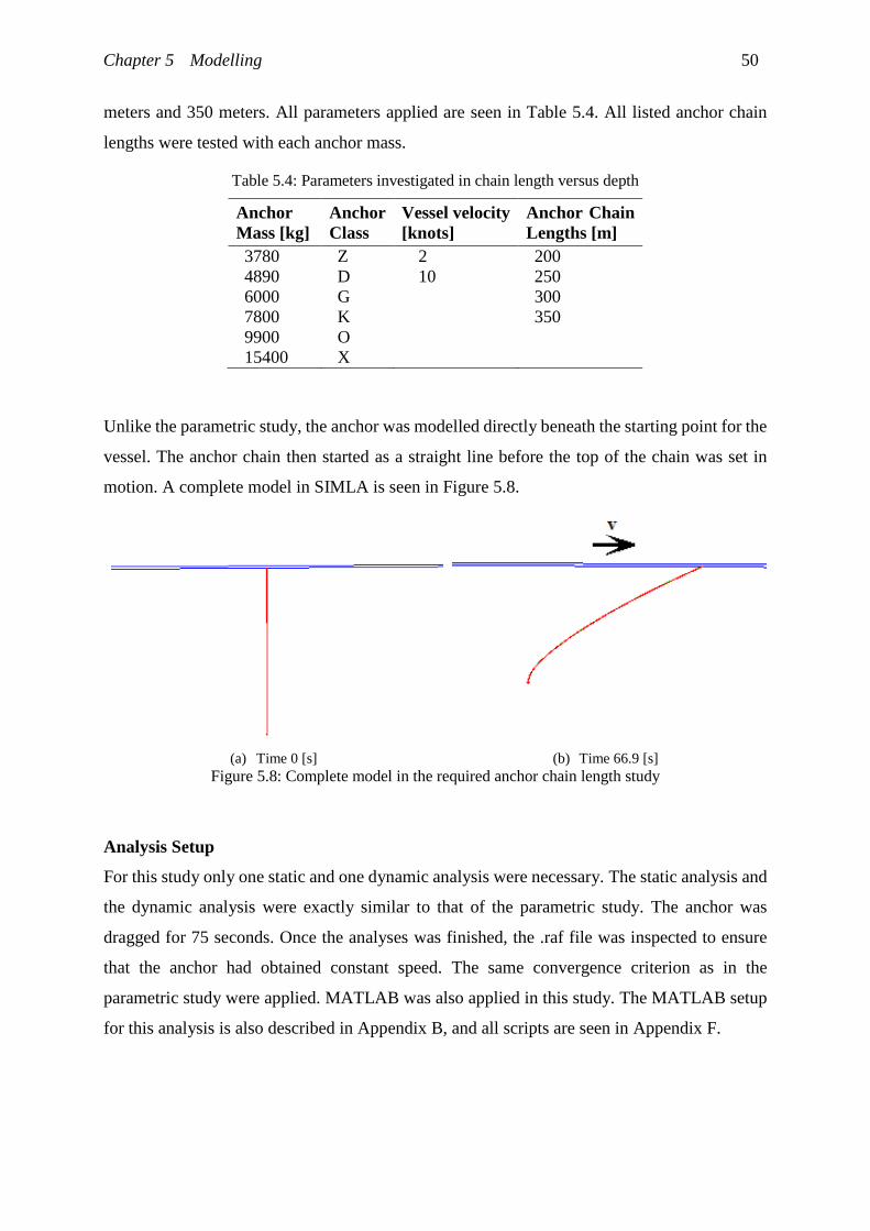
Chapter 5 Modelling 50
meters and 350 meters. All parameters applied are seen in Table 5.4. All listed anchor chain
lengths were tested with each anchor mass.
Table 5.4: Parameters investigated in chain length versus depth
Anchor
Mass [kg]
Anchor
Class
Vessel velocity
[knots]
Anchor Chain
Lengths [m]
3780 Z 2 200
4890 D 10 250
6000 G 300
7800 K 350
9900 O
15400 X
Unlike the parametric study, the anchor was modelled directly beneath the starting point for the
vessel. The anchor chain then started as a straight line before the top of the chain was set in
motion. A complete model in SIMLA is seen in Figure 5.8.
(a) Time 0 [s] (b) Time 66.9 [s]
Figure 5.8: Complete model in the required anchor chain length study
Analysis Setup
For this study only one static and one dynamic analysis were necessary. The static analysis and
the dynamic analysis were exactly similar to that of the parametric study. The anchor was
dragged for 75 seconds. Once the analyses was finished, the .raf file was inspected to ensure
that the anchor had obtained constant speed. The same convergence criterion as in the
parametric study were applied. MATLAB was also applied in this study. The MATLAB setup
for this analysis is also described in Appendix B, and all scripts are seen in Appendix F.

Chapter 5 Modelling 51
5.5.3 Elastoplastic Case Studies
Model Setup
All of the segments modelled in the parametric study were included in the elastoplastic case
studies. The main difference to the parametric study was the modelling of the pipeline. Instead
of 10 meters long, the pipeline was modelled as 10 kilometer. The pipeline was also modelled
with PIPE33 elements, with elastoplastic material properties, instead of PIPE31. The pipeline
was only constrained at the end nodes, meaning the pipeline was allowed to globally deform
and be displaced. As mentioned, extra roller elements were applied, and the anchor was made
extra stiff by applying extra elements.
Eleven cases were analysed. The parameters inspected were chosen based on the results of the
parametric study and the required length of chain study. These results are discussed in
Subchapter 6.1 and 6.2 respectively. The parameters studied are seen in Table 5.5. The
alternative length for the anchor chain was only applied to the 15400 kg anchor, in combination
with varying angles of attack. A complete list of cases studied are seen in
Table 5.6.
Table 5.5: Parameters studied in the elastoplastic study
Anchor
Mass [kg]
Anchor
Class
Pipe Diameter
[Inches]
Vessel velocity
[knots]
Anchor Chain
Length [m]
Angle of
Attack [deg]
9900 O 30 2 660 90
15400 X 40 10 742.5 60
350 30
Table 5.6: Complete list of analyses carried out in the elastoplastic study
Name of models
9900kg200m30in2kn660m90 15400kg200m30in10kn350m90
-660m60 -350m60
9900kg200m30in10kn660m90 -350m30
9900kg200m40in2kn660m90 15400kg200m40in2kn743m90
15400kg200m30in2kn743m90 15400kg200m40in10kn743m90
15400kg200m30in10kn743m90
-743m60

Chapter 5 Modelling 52
Analysis Setup
As the desired output of the analysis was the strain, the VISRES card was applied to gather
information regarding longitudinal strain. The analysis sequence for the elastoplastic study was:
Static, dynamic and dynamic. Unlike the parametric study, there was only one static analysis
sequence. This was because the pipeline was not rotated, as in the parametric study. Instead,
the coordinates of the pipeline, when rotated, were calculated and directly implemented in the
input file. The pipeline was thus in final position when performing the static analysis. The
starting point for the final dynamic analysis was determined by visually inspecting the 3D
visualization. The final restart releases the constraints put on the anchor and anchor chain,
allowing the anchor to move freely and slide. This is equal to the approach in the parametric
study. The same convergence criteria used in the previous studies were applied.
MATLAB was not applied directly in the case studies. All input files are therefore uploaded to
the electronical Appendix F.

53
Chapter 6
6 Results and Discussion
6.1 Parametric Study
The results from the parametric study were gathered by inspecting the 3D visualisation of each
model in XPost. The response of each simulation was categorized by interaction type, and
classified as either realistic or unrealistic.
Several simulations showed unrealistic responses after the contact between the anchor and
pipeline had ceased. The realism of the response was thus evaluated for the anchor-pipeline
interaction itself. The simulation is ruled as unrealistic if the anchor pierces the pipeline, or the
anchor deforms grossly. Small deformations at the tip of the flukes were ignored. The responses
in the non-realistic analyses were included in the results, as the response before the non-real
behaviour was evaluated.
There is no clear consensus on how to define the different responses of an anchor-pipeline
interaction. In DNV-RP-F111 (2010) the interaction between the trawl gear and pipeline are
classified as pull over or hooking, while Wei (2015) classifies the interaction between anchor
and pipeline as either hooking or unhooking. Wei (2015) signifies hooking as any interaction
where the anchor remains in contact with the pipeline for a longer period, this means that sliding
is also defined as hooking.
To categorize the responses seen in the parametric study a new system was developed. The
responses were divided into two main categories: Brief contact and lasting contact. Brief contact
was further divided into two subcategories: Bounce over and pull over. Pull over is when the
anchor remains in contact with the pipeline while being tilted over. An example is seen in
Figure 6.1. A pull over can also occur if the initial impact causes the anchor to twist, and rest
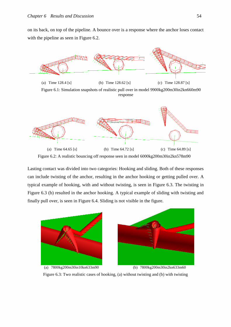
Chapter 6 Results and Discussion 54
on its back, on top of the pipeline. A bounce over is a response where the anchor loses contact
with the pipeline as seen in Figure 6.2.
(a) Time 128.4 [s] (b) Time 128.62 [s] (c) Time 128.87 [s]
Figure 6.1: Simulation snapshots of realistic pull over
response
in model 9900kg200m30in2kn660m90
(a) Time 64.65 [s] (b) Time 64.72 [s] (c) Time 64.89 [s]
Figure 6.2: A realistic bouncing off response seen in model 6000kg200m30in2kn578m90
Lasting contact was divided into two categories: Hooking and sliding. Both of these responses
can include twisting of the anchor, resulting in the anchor hooking or getting pulled over. A
typical example of hooking, with and without twisting, is seen in Figure 6.3. The twisting in
Figure 6.3 (b) resulted in the anchor hooking. A typical example of sliding with twisting and
finally pull over, is seen in Figure 6.4. Sliding is not visible in the figure.
(a) 7800kg200m30in10kn633m90 (b) 7800kg200m30in2kn633m60
Figure 6.3: Two realistic cases of hooking, (a) without twisting and (b) with twisting

Chapter 6 Results and Discussion 55
(a) Time 62.4 [s] (b) Time 62.67 [s] (c) Time 62.84 [s] (d) Time 63.4 [s]
Figure 6.4: Sliding with twist and pull over response in 7800kg200m30in10kn633m30
The defining difference between a hooking and sliding response is that the motion of the anchor
is stopped during hooking. Thus, if the anchor remains in place for several seconds, the response
was registered as hooking, independent of the following behaviour. This is because the eventual
sliding or twisting following a hooking response, are due to increased tension in the cable,
which would have displaced the pipeline. A flowchart showing how the results were categorized
is seen in Figure 6.5.
Figure 6.5: Summary of categorisation

Chapter 6 Results and Discussion 56
6.1.1 Results
Seventy-two models were created and analysed using SIMLA, twelve models created for each
mass, varying the parameters listed in Chapter 5.5.1. The categorisation of each model is seen
in Appendix D. Table 6.1 summarize how many of the models showed realistic, non-realistic
and inconclusive responses.
Table 6.1: Overview of usable results in parametric study
Mass [kg]
3780 4890 6000 7800 9900 15400
Realistic 1 2 6 7 8 12
Non-realistic 11 9 3 3 1 -
Inconclusive - 1 3 2 2 -
Total number
included in results 12 11 9 10 9 12
There were eight models that were inconclusive as the visualization broke after few time steps
and displayed unrealistic behaviour. These are listed in Table 6.2. Seven of the models
encountered numerical issues that were solved by increasing the bending stiffness of the chain
by a factor 10. These are clearly marked in Appendix D. The total number of models taken into
account were 64.
Table 6.2: List of inconclusive models
Inconclusive
4890kg200m40in2kn550m90 7800kg200m40in2kn633m60
6000kg200m40in2kn578m60 7800kg200m40in10kn633m60
6000kg200m40in10kn578m60 9900kg200m40in2kn660m60
-30 9900kg200m40in10kn660m60
To give insight into the trends seen in the results, a ratio system was applied. The ratio was
calculated as seen in Equation (6.1).
𝑅𝑎𝑡𝑖𝑜 =
𝑁𝑢𝑚𝑏𝑒𝑟 𝑜𝑓 𝑟𝑒𝑠𝑝𝑜𝑛𝑠𝑒𝑠
𝑇𝑜𝑡𝑎𝑙 𝑛𝑢𝑚𝑏𝑒𝑟 𝑜𝑓 𝑟𝑒𝑠𝑝𝑜𝑛𝑠𝑒𝑠 [%] (6.1)
For example, the number of responses can be the number of hooking responses for anchors of
15400 kg and angle of attack of 60 degrees, while the total number of responses would then be
the total number of hooking responses. The failed and inconclusive results listed in Table 6.2
are excluded when calculating the ratios.

Chapter 6 Results and Discussion 57
Overall Results
Figure 6.6 shows the distribution of hooking, sliding and brief contact responses for each anchor
mass, while Figure 6.7 shows the distribution of responses within the brief contact category.
The distribution, in addition to bounce over and pull over ratios, are summarized in Table 6.3
for the different anchor masses.
Figure 6.6: Ratio for hooking, sliding and bouncing off
Figure 6.7: Distribution of Brief Contact Ratio seen in Figure 6.6

Chapter 6 Results and Discussion 58
Table 6.3: Response ratios for different anchor sizes
Anchor Mass [kg]
3780 4890 6000 7800 9900 15400
Hooking 0 % 0 % 14 % 20 % 10 % 50 %
Sliding 8 % 9 % 29 % 40 % 40 % 33 %
Bounce over 83 % 82 % 43 % 20 % 10 % 17 %
Pull Over 8 % 9 % 14 % 20 % 40 % 0 %
Sum 100 % 100 % 100 % 100 % 100 % 100 %
Effect of angle of attack
Three angles of attack were applied: 90 degrees, 60 degrees and 30 degrees. Figure 6.8 shows
the hooking ratios for different angles of attack and anchor masses. Figure 6.9 shows the sliding
ratio for different angles and anchor masses.
Figure 6.8: Hooking ratio depending on angle of attack and anchor mass

Chapter 6 Results and Discussion 59
Figure 6.9: Sliding ratio depending on angle of attack and anchor mass
Effect of angle of attack, pipe size and vessel velocity
There were no hooking responses when the angle of attack was 30 degrees. This angle was
therefore excluded when inspecting hooking ratio. A complete summary of how angle of attack,
pipe size, vessel velocity and anchor mass affects the hooking ratios is seen in Table 6.4.
Similarly, there were no sliding responses for the 60 and 90 degrees angle of attack, and they
were hence excluded when inspecting sliding. Table 6.5 shows the effect of pipe size, vessel
velocity and anchor mass on the sliding ratio when the angle of attack was set to 30 degrees.
Table 6.4: Hooking ratio distribution for all parameters, excluding 30 degrees
Angle of
attack
[Degrees]
Pipe
Size
[Inches]
Vessel
Velocity
[Knots]
Anchor Mass [kg]
3780 4890 6000 7800 9900 15400 SUM
90
30 2 - - - - - 10 % 10 %
10 10 % 10 % 20 %
40 2
10
60
30 2 10 % 10 % 10 % 10 % 40 %
10 10 % 10 %
40 2 10 % 10 %
10 10 % 10 %
SUM 10 % 20 % 10 % 60 % 100%

Chapter 6 Results and Discussion 60
Table 6.5: Sliding ratio distribution for all parameters excluding, 60 and 90 degrees
Angle
[Degrees]
Pipe Size
[Inches]
Velocity
[Knots]
Anchor Mass [kg] SUM
3780 4890 6000 7800 9900 15400
30
30 2 6 % 6 % 6 % 6 % 6 % 6 % 38 %
10 6 % 6 % 6 % 19 %
40 2 6 % 6 % 6 % 25 %
10 6 % 6 % 6 % 19 %
SUM 6 % 6 % 13 % 25 % 25 % 25 % 100 %
The effect of pipe size and velocity on hooking is seen in Figure 6.10, with figure (a) showing
the hooking ratio for different vessel velocities and pipe sizes, with an angle of attack of 90
degrees, and figure (b) showing with an angle of attack of 60 degrees. Figure 6.11 summarises
the effect of pipe size and vessel velocity on the sliding ratio when the angle of attack is 30
degrees.
(a) Depending on pipe size and angle of attack (b) Depending on pipe size and vessel velocity
Figure 6.10: Hooking ratio depending on pipe size and vessel velocity
Figure 6.11: Sliding ratio depending on pipe size and vessel velocity

Chapter 6 Results and Discussion 61
6.1.2 Discussion
General Findings
The general trend points towards an increase in hooking and sliding with increased mass of
anchor, lower vessel speed and smaller pipe diameter. The largest amount of hooking occurs
for an angle of attack of 60 degrees. All hooking occurrences for the 60 degrees cases were
caused by anchor twisting and getting hooked on the side, as seen in Figure 6.3 (b). None of the
models displayed a hooking response when the angle of attack was 30 degrees, while all cases
of sliding were registered for this angle of attack.
The trend of a higher hooking ratio when larger anchors interact with smaller pipes, at a low
velocity, was also found by Vervik (2011) and Wei (2015). However, comparing results do
pose several issues as Wei (2015) uses vessel speeds of 6 and 12 knots, and different outer pipe
diameter. Despite this, the same conclusion is drawn that more hooking occur for lower
velocities, and smaller pipes.
There is some discrepancy when comparing the results with the geometric calculations by
Vervik (2011), using Equation (3.13), for the 90 degree angle of attack. According to Vervik
(2011), any anchor larger than 4580 kg should hook onto a pipeline with a total diameter of
0.86 meters, and any anchor larger than 13500 kg should hook onto a pipeline with a total outer
diameter of 1.12 meter. An outer diameter of 0.86 meters corresponds to a coated 30-inch
pipeline, and 1.12 meter corresponds to a coated 40-inch pipeline. The results obtained in the
parametric study suggest that 13500 kg would not be sufficient for the 40-inch pipeline, as the
15400 kg anchor did not hook. Furthermore, the smallest anchor to hook onto the 30-inch
pipeline was the 7800 kg anchor, which is larger than the predicted 4580 kg anchor. This
indicates that geometry alone cannot predict hooking.
A reason for this discrepancy is that the geometry approach done by Vervik (2011) does not
consider alternative attack points on the pipeline. Neither does it consider how the attack point
for the anchor is influenced by vessel velocity, length of anchor chain, pipe size and soil
stiffness. The difference in the anchors’ position just before impact, is seen in Figure 6.12.
There is a notable difference in how the anchor impacts with the pipeline in Figure 6.12 (b) and
(d).

Chapter 6 Results and Discussion 62
(a) 4890kg200m30in2kn550m90 (b) 4890kg200m30in10kn550m90
(c) 15400kg200m30in2kn743m90 (d) 15400kg200m30in10kn743m90
Figure 6.12: Snapshots showing the effect of size and velocity on attack point
There are also some discrepancies when comparing with Wei (2015), mainly when it comes to
the amount of hooking scenarios. When comparing results that are quite similar, Wei (2015)
reports hooking for many cases that were not registered as hooking in this study. The fact that
Wei (2015) has used different categories makes it problematic to compare the results. It is
difficult to pinpoint the reason for the difference in results, as the input files used by Wei (2015)
were not available. However, Wei (2015) defined sliding as a hooking response, this may be
part of the explanation why Wei (2015) obtained more hooking responses. Furthermore, it is
seen that many of the cases Wei (2015) reported as hooking, were categorized as pull over in
this study.
The results from this study indicate that the pull over ratio increases with larger anchor mass
until the anchor weight reaches 15400 kg. The 15400 kg anchors however, has a drastic increase
in hooking ratio, which explains why there were so few cases of pull over. The increase in pull
over ratio with increasing mass may be caused by the combination of increased mass of anchor
and chain, and the increase in chain length. This combination results in the anchor chain laying
on the seabed after having passed the pipeline, and pulling the anchor downwards instead of
upwards. The direction of the forces pulling on the anchor, the large distributed mass of the
system and the high friction factor between anchor and pipeline, are most likely the reasons for
the pull over response.

Chapter 6 Results and Discussion 63
Despite the difficulties in comparing results, the general trend that hooking increases with
anchor geometry, lower vessel velocities and smaller pipe diameter, are the same seen in the
theses by Vervik (2011) and Wei (2015)
Sources of Error
There were several sources of error when performing the parametric study. This section is
dedicated to describing these, their effects on the result and possible remedies.
The results were gathered by visual inspection of the 3D visualization of the models. This
presents a possibility for erroneous classification. This is particularly relevant for the unrealistic
models, as the moment where the model went from being realistic to unrealistic had to be
located visually. The categorization of the response was then based on the realistic part.
In general, there are more unrealistic responses for the smaller anchors. The short chain length
could be the cause of this, as the short length results in the anchors having a different attack
point than with longer chain lengths. This effect is enhanced with higher velocities, as seen in
Figure 6.12 (a) and (b). Anchors of 3980 kg and 4890 kg had a tendency to reach the pipeline
with the flukes first when the velocity was 10 knots, as seen in Figure 6.12 (b). This resulted in
the tip of the flukes penetrating the pipewall and deforming in an unrealistic manner. This is
also one of the reason there were fewer unrealistic responses for the larger anchors.
The flukes penetrating the pipeline is most likely due to numerical error with SIMLA. The
contact element placed on the pipeline does not register the contact between the fluke tips and
the pipeline early enough. This effect was one of the main contributors to the unrealistic results,
as the flukes would penetrate the pipeline, and be forced back with such a force that the anchor
would bounce over and deform. This could possibly have been amended by applying several
small roller elements along the circumference of the pipeline, which would be able to register
the contact with the fluke tips.
Furthermore, several of the anchors showed signs of small deformation of the flukes. This could
have been prevented by applying extra elements along the flukes and shank, with extra bending
stiffness, as described in Subchapter 5.5.1. This was not discovered early enough, so the
parametric study was performed without the extra elements. However, to investigate if extra
elements with extra bending stiffness would solve the problem, seven of the models were
reanalysed with the new elements. The general trend of these analyses were that the anchor did
not deform, and the anchor displayed the same behaviour as registered.

Chapter 6 Results and Discussion 64
Another important source of error was related to one of the constraints on the pipeline. The
constraint that was supposed to allow for alterations of the span height, had been set to zero,
instead of removed when the span height was zero. This results in the pipeline not penetrating
the seabed in a realistic manner, but resting on top of the it. This is clearly seen in Figure 6.12.
Had this constraint not been present, the pipeline would have settled realistically onto the
seabed due to its weight. As the effect of the span height was not studied, this error was not
discovered before the end of the project, and was not corrected. It is uncertain how much this
affects the results, but it will have had an effect on the attack point on the pipeline.
The chosen run time for the analysis will also have affected the outcome of the study. This is
particularly relevant for the sliding scenarios, where a longer time span might have resulted in
the anchor beginning to twist and finally pull over, or hook onto the pipeline. However, due to
time limits and only applying four roller elements, this was not investigated in the study.
6.2 Minimum Chain Length
A total of 48 models were created and analysed. Each analysis ran for 75 seconds. The nodal
velocity for anchors node 40022 in Y- and Z-direction is seen for the 10 knot case in
Figure 6.13. The velocities obtain constant values, but become unrealistic the last five seconds.
The error, which occurred when towing at both 2 and 10 knots, was caused by towing velocity
being defined for 70 seconds in the .sif file. Because of this, all results after 70 seconds are
ignored for both the 2 knot and the 10 knot scenario.
(a) Nodal velocity in Y-direction (b) Nodal velocity in Z-direction
Figure 6.13: Error in nodal velocities in Y- and Z-direction

Chapter 6 Results and Discussion 65
6.2.1 Results
The general trends in the 2 knot and 10 knot models are seen in Figure 6.14 and Figure 6.15
respectively. The Z-coordinates for the chain element connected to the anchor, at the 70 second
mark, are summarized in Table 6.6 and Table 6.7, for 2 and 10 knots, respectively.
Figure 6.14: Chain shape for different lengths after 70 seconds with 2 knot velocity
Table 6.6: Final Z-coordinate for chain element connected to anchor with 2 knots
Chain
Length [m]
Anchor Mass [kg]
3870 4890 6000 7800 9900 15400
200 -196.4 -196.8 -197.1 -197.4 -197.7 -198.3
250 -246.3 -246.6 -246.9 -247.2 -247.5 -248.0
300 -296.4 -296.7 -296.9 -297.2 -297.5 -297.9
350 -346.5 -346.7 -346.9 -347.2 -347.5 -347.9

Chapter 6 Results and Discussion 66
Figure 6.15: Chain shape for different lengths after 70 seconds with 10 knot velocity
Table 6.7: Final Z-coordinates for chain element connected to anchor with 10 knots
Chain
Length [m]
Anchor Mass [kg]
3870 4890 6000 7800 9900 15400
200 -96.1 -93.8 -101.7 -99.3 -102.6 -109.1
250 -132.2 -143.8 -137.3 -140.2 -143.9 -150.4
300 -180.4 -182.9 -185.1 -198.4 -191.4 -197.6
350 -240.5 -237.3 -236.5 -239.2 -242.2 -248.0
6.2.2 Discussion
The general trend was, as predicted by Equation (2.2) in Chapter 2.2, that the larger the velocity,
the larger the drag forces on the anchor chain. These forces resulted in the anchor being lifted
vertically as it was towed. This can be seen in Figure 6.15. This trend was also seen in the work
of Vervik (2011) who applied SIMLA, and the same drag coefficients, to study the effect of
several velocities on anchor chain being towed.
To estimate the minimum chain length for the anchor to interact with the pipeline, it was
assumed that there was a linear connection between the coordinates for the anchor chain above
and below the seabed. This is a simplified approach as it completely neglects the shape of the
towed chain, and the lumped mass at the end. However, it is adequate for the purpose of finding
minimum length of chain. The simplification is seen in Figure 6.16 where (y0, z0) are the

Chapter 6 Results and Discussion 67
coordinates for the anchor chain stopping above the seabed, and (y1, z1) for the anchor chain
below the seabed.
The recommended new length of the anchor chain was found by use of Equation (6.2). The
minimum length for the anchor chain for the two velocities are presented in
Table 6.8.
Figure 6.16: Simplified assumption of geometry for two anchor chain coordinates
𝑙𝑙 =
𝐿
cos(ϕ) (6.2)
Table 6.8: Minimum required anchor chain length
Minimum
length [m]
Anchor Mass [kg]
3870 4890 6000 7800 9900 15400
2 Knot 203.62 203.24 202.94 202.58 202.26 201.74
10 Knot 321.05 318.11 315.58 301.62 309.06 302.56
Despite the results showing the same trend as Vervik (2011), the conclusion that 70 seconds
was sufficient to get a state of equilibrium in the system, and find the required length of the
anchor, has proven to be false. Despite obtaining constant velocity, it was later observed that
the results obtained are only applicable if the distance between pipeline and the anchor’s starting
point is less than 100 meters. In hindsight, the acceleration of the nodes should have been
investigated instead of the velocity. The Z-coordinates could then be determined at the time
where acceleration in both vertical and horizontal direction was zero, as that would be the time

Chapter 6 Results and Discussion 68
of equilibrium in the system. However, the results can still be applied as long as the distance
between the pipeline and the anchor is less than 100 meters.
6.3 Elastoplastic Case Studies
The eleven cases inspected were chosen based on the results from the previous two studies.
There were two motives behind this study. The first, to investigate how well the anchor’s
response had been predicted in the parametric study. The second, to inspect the pipeline’s
response, by investigation whether or not the longitudinal strain in the cross-section exceeded
DNV’s criteria.
The design criteria for local buckling, when the pipeline is exposed to combined loading, is
expressed in Equation (3.4) and (3.5). It was assumed that there would be external overpressure,
and hence Equation (3.5) was chosen. A conservative assumption was made, assuming that the
pressures in Equation (3.5) would be insignificant, and the contribution from these were set to
zero. By further assuming a high safety class, and ignoring the contribution from corrosion on
the thickness, the characteristic bending strain resistance was calculated using Equation (3.6).
The values for the factors needed in this calculation, and the result, can be seen in Table 6.9.
Table 6.9: Calculation of characteristic bending strain resistance
Description Symbol Value
Resistance strain factor 𝛾𝜀 3.3
Material resistance factor 𝛾𝑚 1.15
Safety class resistance factor 𝛾𝑆𝐶 1.26
Train hardening 𝛼ℎ 0.93
Girth weld factor 𝛼𝑔𝑤 0.82
Thickness/diameter ratio 𝑡2𝐷
1
35
Characteristic bending strain resistance 휀𝑐(𝑡2,0) 0.01324
Design loads strain 휀𝑆𝑑 0.00401
The responses were categorized as describe in Subchapter 6.1, with the additional requirement
that hooking must result in the pipeline being globally displaced. An example of a hooking
scenario in the elastoplastic study, is seen in Figure 6.17 and Figure 6.18. Figure 6.17 shows
the configuration of the system before impact, and Figure 6.18 shows the system’s
configuration during hooking.
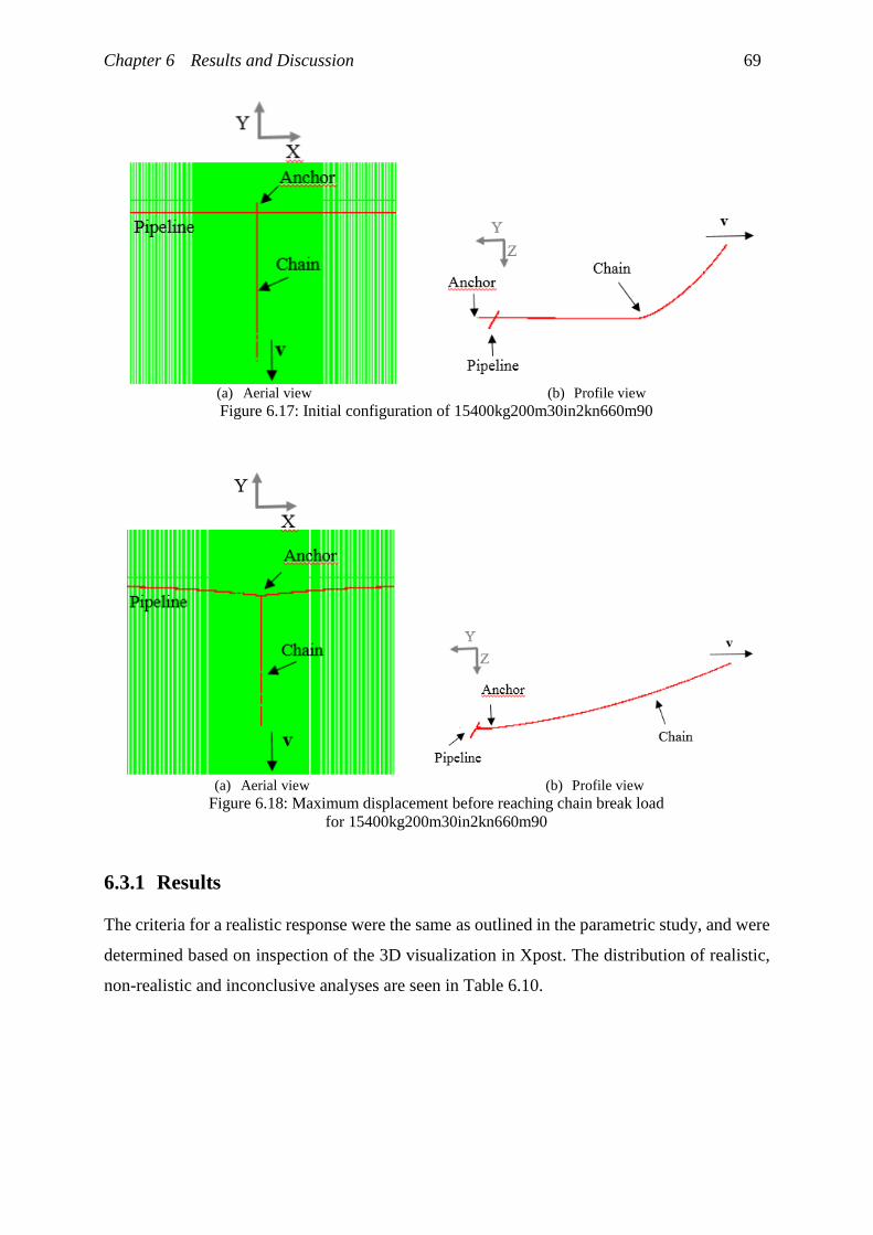
Chapter 6 Results and Discussion 69
(a) Aerial view (b) Profile view
Figure 6.17: Initial configuration of 15400kg200m30in2kn660m90
(a) Aerial view (b) Profile view
Figure 6.18: Maximum displacement before reaching chain break load
for 15400kg200m30in2kn660m90
6.3.1 Results
The criteria for a realistic response were the same as outlined in the parametric study, and were
determined based on inspection of the 3D visualization in Xpost. The distribution of realistic,
non-realistic and inconclusive analyses are seen in Table 6.10.

Chapter 6 Results and Discussion 70
Table 6.10: Overview of usable results in elastoplastic study
Mass [kg]
9900 15400
Anchor Chain Length [m] 660 743 350
Realistic 1 4 2
Non-realistic 3 - 1
Inconclusive - - -
Total cases studied 4 4 3
In all of the non-realistic cases, the anchor penetrated the pipewall. However, this was after a
few seconds of contact, which were used as results.
The strain in the pipeline’s cross-section, were found from plots created in XPost. Eight Gauss
points were applied in the calculations. For the results, strain was inspected at Gauss point 1
and 5, as their location was deemed the most critical for the response. Their location on the
cross-section of the pipeline is shown in Figure 6.19, where the anchor is moving in positive
Y-direction.
Figure 6.19: Gauss points on the cross-section
The strain plots were compared with the characteristic bending strain resistance, and the design
load criteria. If the chain’s breaking load was exceeded, the strain values were determined at
the time step where the chain would have broken. The response of the anchor and pipeline were
documented, and the anchor’s response compared to the one found in the parametric study. The
longitudinal strain plots, and a complete table containing the results, are found in Appendix E.
Table 6.11 summarizes the most important findings.

Chapter 6 Results and Discussion 71
Table 6.11: Summary of results in Elastoplastic Study
Model Name Anchor Response
Comparison
with parametric
study
Strain design
load
exceeded
9900kg200m30in2kn660m90 Bounce over Dissimilar No
-660m60 Twist and slide Dissimilar No
9900kg200m30in10kn660m90 Bounce over Dissimilar No
9900kg200m40in2kn660m90 Bounce over Similar No
15400kg200m30in2kn743m90 Hooks Similar Yes
15400kg200m30in10kn743m90 Hooks Similar Yes
-743m60 Twist and pull over Dissimilar No
15400kg200m30in10kn350m90 Hooks Similar Yes
-350m60 Twist and slide Dissimilar No
-350m30 Twist and slide Dissimilar No
15400kg200m40in2kn743m90 Bounce over Similar No
For the three hooking responses, the maximum displacement of the pipeline was found by
locating the time step where maximum chain breaking load was reached, and reading of the
displacement in Y- and Z-direction from the 3D visualization. The results are presented in
Table 6.12.
Table 6.12: Global displacement of roller element
Global Displacement
Model Name Y-direction [m] Z-direction [m]
15400kg200m30in2kn660m90 58.94 -0.66
15400kg200m30in10kn743m90 6.50 -1.03
15400kg200m30in10kn350m90 39.29 5.13
6.3.2 Discussion
Ideally, all the parameter combinations inspected in the parametric study should have been
studied with a full-length elastoplastic pipeline. The trends that are discussed here are thus
based on the eleven cases. It is therefore not possible to draw any overall conclusion about how
accurately the parametric study manages to predict the anchor’s response.
The general trend of the results imply that in the case of hooking, the longitudinal strain in the
pipeline’s cross-section will exceed DNV’s design load and the characteristic resistance strain.
This indicates that hooking exposes the cross-section to local buckling. This is the same trend
as observed by Al-Warthan et al. (1993), when inspecting hooking on a 16-inch pipeline.

Chapter 6 Results and Discussion 72
Furthermore, the results indicate that the strain did not exceed the design load, nor the
characteristic strain, before having displaced the pipeline a minimum of 3 meters. This is in
accordance with the results obtained by Sriskandarajah and Wilkins (2002).
The hooking scenarios supports the parametric study’s conclusion that an anchor of 15400 kg
is not large enough to hook onto a 40-inch pipeline, contradicting the results from the geometric
consideration done by Vervik (2011). The case studies further support the conclusion from the
parametric study that hooking occurs more frequently for smaller pipelines, as no hooking
occurred for the cases applying a 40-inch pipeline.
The displacement of the pipeline shown in Table 6.12, indicate that at lower velocities, the
pipeline will be displaced farther, before the anchor chain reaches its breaking load of 6.69 MN.
This is the same trend reported by Vervik (2011). The 2 knot case shows a slower increase in
anchor chain load, as is seen in Figure 6.20 (a), compared to the rapid increase in figure (b)
where the anchor is towed at 10 knots. This slow increase in axial force, in the chain element,
is due to the low velocity, shape of chain and amount of chain in contact with the seabed.
(a) 15400kg200m30in2kn743m90 (b) 15400kg200m30in10kn743m90
Figure 6.20: Element force in anchor chain element 50002
red dot indicates point of anchor chain breaking load
For both of the hooking cases where the chain length was at its maximum, the pipeline was not
lifted of the seabed. However, for the case with 350 meter long chain, the pipeline was lifted
approximately 5 meters vertically. The 350 meter case also displaced the pipeline further
laterally, than the case applying maximum chain length of 743 meters. This indicates that the
length of anchor chain is of significance for the pipeline’s response. These results support the
claim by Sriskandarajah and Wilkins (2002) that the consequences are worse when the anchor
is towed without the chain resting on the seabed.

Chapter 6 Results and Discussion 73
The negative vertical displacement in the hooking scenarios, seen in Table 6.12, indicate that
the pipeline was dragged downwards into the soil. Realistic modelling of the soil was outside
the scope of this work. Since this response is heavily dependent on the soil properties, it is
recommended that the soil modelling should be improved in the future.
Contrary to the parametric study, the cases studied indicate no hooking response for the 60
degrees angle of attack. None of the three cases with this angle displayed any sign of hooking.
A possible explanation for this is that in the case studies, pipeline displacement was allowed.
The initial impact, combined with the anchor twisting, resulted in the pipeline being displaced,
which reduces the pipelines ability to stop the motion of the anchor. The prolonged contact seen
in the parametric study was therefore not observed in the elastoplastic cases.
In general, the parametric study was good at predicting hooking, when the angle of attack was
90 degrees. The pull over response was however not seen despite being predicted for the two
cases 9900kg200m30in2kn660m90 and 9900kg200m30in10kn660m90. In all cases of brief
contact, the anchor appeared to bounce over, rather than pull over. This raises some questions
regarding the realism of the pull over response.
Finally, there are two issues regarding the modelling that should be noted. The first is that the
friction between the anchor chain and pipeline was removed from the study, as the friction
caused the pipeline to roll back and forth on the seabed. This caused instability in the system,
and erroneous result. Due to time limitations, the friction between chain and pipeline was hence
excluded. This friction could possibly have large effects on the pipelines and anchors response,
and should be included in future studies.
The second issue concerns the models showing non-realistic behaviour. These cases all struggle
with the same problem as seen in the parametric study, namely that the anchor flukes pierced
the pipeline. The proposed remedy in subsection 6.2.2, applying several smaller roller elements
along the circumference of the pipe, is also applicable here.
In general, the eleven cases studied support the conclusions drawn in the parametric study, that
probability for hooking increases with larger anchor sizes, smaller pipelines and lower
velocities. The cases studied also indicate a large probability for local buckling, when the
anchor hooks onto the pipeline. This is accordance with the research done by Al-Warthan et al.
(1993) and Sriskandarajah and Wilkins (2002). The results did however raise some questions
regarding the hooking response, when the angle of attack was 60 degrees, and the pull over
response in general.


75
Chapter 7
7 Conclusion
The anchor’s response to an interaction with the pipeline was categorized as either brief or
lasting contact in the parametric study. Brief contact encompasses the pull over and bounce
over responses, and lasting contact includes sliding and hooking. Having categorized the
responses in the parametric study, certain trends appeared. The results indicate that there is a
larger probability for hooking with reduced vessel speed, smaller pipe diameter and larger
anchors. This is in accord with the results found by Vervik (2011) and Wei (2015). The results
from the eleven elastoplastic cases studied support this finding, by demonstrating that anchor
hooking only occurs for the 30-inch pipe size. The results from the parametric study, and the
eleven cases studied, also indicate that only inspecting the geometry of the anchor to predict a
hooking scenario, as done by Vervik (2011), is not sufficient.
The minimum chain length study displayed that, due to drag forces exerted on the anchor chain,
the minimum chain length was much larger at higher velocities. For the vessel towed at 2 knots,
a chain approximately 3 meters longer than the water depth is required. For the 10 knot case
the drag forces were much greater. The minimum chain length in this case must be at least
110 meters longer than the water depth. These results are however only valid when the anchor
is dropped 100 meters away from the pipeline, due to the analyses not being provided enough
runtime.
The parametric study indicated that the largest probability for hooking was for an attack angle
of 60 degrees. This result was not found in the eleven case studies, where hooking only occurred
for an angle of attack of 90 degrees. This might indicate that the hooking response, found in the
parametric study, for an angle of attack of 60 degrees, is a result of the rigid body modelling of
the pipeline, rather than the actual anchor’s response.

Chapter 7 Conclusion 76
All of the cases with full-length pipeline, which resulted in hooking, indicate that the
longitudinal cross-sectional strain exceeds DNV’s load design criteria, before the axial load in
the chain surpasses its breaking load. The longitudinal strain in these cases also exceed the
characteristic strain resistance. The exceedance of DNV’s design criteria, and characteristic
strain resistance, puts the pipeline at risk for local buckling.
The results from the eleven case studies also indicate that the pipeline is displaced laterally, a
minimum of 3 meters, before exceeding the characteristic bending strain. This is in accordance
with the results of Sriskandarajah and Wilkins (2002), who demonstrated that a much smaller
force was needed to initiate lateral displacement, compared to local buckling.
The case studies that resulted in the anchor hooking also reveal that the global displacement of
the pipeline is much greater when the anchor is towed at a lower velocity. For higher velocities,
the hooking case with minimum chain length, displaced the pipeline farther, both laterally and
vertically, than the anchor towed with maximum chain length. This demonstrates that the
consequences are worse when the anchor is towed with minimum required chain length, as
claimed by Sriskandarajah and Wilkins (2002).

77
Chapter 8
8 Further Work
The three hooking cases that exceeded DNV’s design load criteria and characteristic resistance
strain, indicate that the pipeline’s cross-section is exposed to failure mechanisms, such as local
buckling. A detailed FEA is necessary to determine which of the failure mechanisms would
occur when exceeding the critical strain. The protective effect of the pipeline’s coating should
be included in such a study of the local effects of the impact.
A more detailed FEA study would allow for the inspection of the effect the attack point of the
anchor has on the pipeline’s response. That is, how would the pipeline’s response differ if the
anchor hits with the flukes first, or with the shank. Such a study would also give a better
understanding of the dangers of brief contact. The brief contact responses could cause damage
to the coating, which after time would develop into leaking or rapturing of the pipeline. A
fatigue study of a pipeline damaged by brief contact might therefore be of interest.
It could also be of interest to study the pull over response in more detail. The pull over response
was not seen in the eleven cases studied, so it is uncertain if this response is realistic. An analytic
study of the pull over response could possible determine the realism of the response.
It is recommended that the focus of future work should be on the study of the pipeline’s local
response. This should be done by creating a local and detailed FEA, taking in account
behaviours such as post-yield and bifurcation, and studying both the immediate reaction to the
interaction and the long-term effect.


79
Bibliography
Al-Warthan, A. I., Chung, J. S., Huttelmaier, H. P., & Mustoe, G. G. W. (1993). Effect of Ship
Anchor Impact In Offshore Pipeline.
Belytschko, T., Liu, W. K., Moran, B., & Elkhodary, K. I. (2014). Nonlinear Finite Elements
for Continua and Structures - Second Edition: Wiley.
Damage to Submarine Cables Caused by Anchors. (2009). International Cable Protection
Committee.
DNV-OS-E301. (2010). DNV Offshore Standard - Position Mooring. Høvik.
DNV-OS-F101. (2013). DNV Offshore Standard - Submarine Pipeline System. Høvik.
DNV-RP-F111. (2010). DNV Recommended Practice - Interference Between Trawl Gear and
Pipelines. Høvik.
DNV Energy Report. (2010). Recommended Failure Rates for Pipelines (2009-1115).
Retrieved from Høvik: https://www.dnvgl.com/oilgas/publications/reports.html
DNV Rules for Classification of Ships, P. C. (2011). Hull Equipment and Safety. Høvik.
Faltinsen, O. M. (1990). Sea Loads on Ships and Offshore Structures. Cambridge: Cambridge
University Press.
Gjertveit, E., Berge, J. O., & Opheim, B. S. (2010). The Kvitebjorn Gas Pipeline Repair. Paper
presented at the Offshore Technology Conference Houston, Texas.
HSE. (2009). Guidelines for Pipeline Operators on Pipeline Anchor Hazards. Aberdeen.
Kyriakides, S., & Corona, E. (2007). Mechanics of Offshore Pipelines, Volume I: Buckling and
Collapse: Elsevier.
Langen, I., & Sigbjörnsson, R. (Eds.). (1986). Dynamisk Analyse av Konstruksjoner: Tapir.

Bibliography 80
MARINTEK. (2012). Fact Sheet - SIMLA. Retrieved from
https://www.sintef.no/globalassets/upload/marintek/pdf-filer/factsheets/simla.pdf
Moan, T. (2003a). TMR4190 Finite Element Modelling and Analysis of Marine Structures.
Trondheim: Department of Marine Technology, Norwegian University of Science and
Technology.
Moan, T. (Ed.) (2003b). TMR4190 Finite Element Modelling and Analysis of Marine Structures
- Chapter 12 Nonlinear Analysis. Trondheim: Department of Marine Technology,
Norwegian University of Science and Technology.
SOTRA. (2014a). Stockless Anchors. Retrieved from
http://www.sotra.net/products/anchors/stockless-anchors
SOTRA. (2014b). Studlink - Common Link. Retrieved from
http://www.sotra.net/products/chains/studlink-common-link
Sriskandarajah, T., & Wilkins, R. (2002). Assessment of Anchor Dragging On Gas Pipelines.
Sævik, S. (2008). SIMLA - Theory Manual (700254.00.01). Retrieved from Trondheim:
MARINTEK
Sævik, S. (2014). Lecture Notes in Offshore Pipeline Technology. Trondheim: Department of
Marine Technology, Norwegian University of Science and Technology.
Sævik, S., Økland, O. D., Baarholm, G. S., & Gjøsteen, J. K. Ø. (2010). SIMLA Version 3.15.0
User Manual. Trondheim: Norwegian Marine Technology Research Institute
Vervik, S. (2011). Pipeline Accidental Load Analysis. (Master), NTNU, Trondheim.
Wei, Y. (2015). Anchor Loads on Pipelines. (Master), NTNU, Trondheim. (200.10.06.15)
Wong, M. B. (2009). Chapter 2 - Plastic Behavior of Structures Plastic Analysis and Design of
Steel Structures (pp. 55-80). Boston: Butterworth-Heinemann.

I
Appendix
Appendix A Alterations done to Wei’s Model for
Parametric Study
The original short model received from Ying Wei (2015), was a draft, and not the finished
product used in Wei’s parameter study. This is one of the main reasons it is difficult to compare
results obtained in this thesis. What follows is a list of alterations done to create the models in
the parameter study. Line numbers listed below refer to the draft received from Wei.
General changes
Wei performs one static analysis followed by a dynamic analysis. In the parametric
study performed in this thesis this has been altered to one static analysis, followed by
one static analysis allowing rotation of the pipeline, then one dynamic analysis and lastly
sliding is allowed through a new restart of the dynamic analysis. The TIMECO cards
were therefore updated to include two static TIMECO cards followed by four dynamic
TIMECO cards, instead of one static and three dynamic.
Anchor changes
Anchor geometry is updated by calculations performed in AnchorCoor.m in accord with
anchor mass. Line 20 through 24 is updated with the new information.
The flukes are modelled as one element group per fluke, instead of as one. Line 26
through 28 is updated to create these element groups. The lines will now have been
shifted.
The distributed mass and outer diameter of the anchor is updated by updating the
ELPROP card for the anchor element groups. The calculations necessary are performed
in the AnchorCoor.m. Lines 37, 38 and 39 are updated, and a new line is created for the
new element group.

Appendix A Alterations done to Wei’s Model for Parametric Study II
The anchor geometry defined by NODPROP is updated. That is, lines 40-63 are
updated.
Cable changes
The cable is modelled by 1000 elements instead of 230. The cable is divided into three
segments instead of four. Each segment is of equal length, but has a different number
of elements. In the first segment the first element lengths are equal to 6*chain diameter.
The remaining amount of elements are divided in three, 2/3 of the elements are used on
the second segment, and 1/3 of the elements are on the last segment. The length of each
segment will thus vary. Line 76-86 is altered.
Line 88, ELCON card is updated as the number of elements are updated from 230 to
1000.
Lines 94 and 96 are updated, that is the ELPROP card and MATERIAL card. All
relevant calculations are performed in CableCoor.m. That is the cable distributed mass
and submerged mass, and outer diameter. Bending, axial and torsional stiffness is
updated in accord with the calculations.
Pipeline changes
Lines 115, ELPROP card is updated with correct outer diameter, thickness, distributed
dry and submerged mass calculated in PipeMass.m.
A new line is inserted to model the rotation of the pipeline. This is done with a CONSTR
card. A new time history was created for this rotation. The pipeline is fully rotated
before the onstart of the dynamic analysis.
Seabed changes
New contact element groups had to be made for the two fluke segments. In addition, a
new contact element was created for the cable.
The contact elements for the cable were rotated by 90 degrees by use of ELORIENT.
The friction coefficient defined in the MATERIAL card were altered from 0.3 in X-
direction to 1.0.

Appendix A Alterations done to Wei’s Model for Parametric Study III
The maximum value for the material curve for soily was reduced to make the soil slightly
softer.
Roller/Contact element changes
Ying Wei had for the short model modelled the roller elements as small roller elements
along the cross-sectional area of the pipeline. This was replaced with four roller element
groups, modelled as 100 meter long and attached to the pipeline.
The contact between the cable and the pipeline was updated from CONTACT to
ISOCONTACT with friction coefficient of 0.38.
Sliding Analysis
Each model requires a different restart of the sliding analysis.
To allow sliding boundary conditions and constrains were adjusted. All boundary
conditions for the anchor are released, that is lines 71, 72 and 73 had to be altered. The
anchor elements are constrained in direction 1 by constraining the fluke to the shank.
All cable elements are also released in direction 1, with the exception of the top element.


V
Appendix B Structure of MATLAB scripts
Parameter Study
An unfinished model created by Wei (2015) was the starting point for the models. This model
was altered using FlexEdit and made into a standard input file that could easily be altered using
MATLAB. A list of all alterations is presented in Appendix A. What follows is a description of
the MATLAB scripts created to perform the parametric study efficiently. These are presented
so that if it is desirable to inspect other parameters than those in this study, it is easily done.
The RunSIMLAMainFile.m script is created such that it writes the .sif file by collecting
information regarding the parameters from two Excel sheets, performing relevant calculations
and substituting lines in the standard input model before executing the SIMLA analysis. The
general structure of the MATLAB script is summarised in Figure B.1 and is described below.

Appendix B Structure of MATLAB scripts VI
Figure B.1: Structure of MATLAB script, parametric study
InputRun.m starts with collecting relevant information regarding which model to create from
“InputAnalysis”. This Excel-document contains information about anchor mass, pipe diameter,
vessel velocity and angle of attack. Water depth is defined in InputRun.m, and this script also
present the possibility for the user to define a chain length. InputRun.m then executes the
function RunSIMLAMainFile.m that in return executes ReadingAncorInput.m, which collects
the anchor geometry, maximum chain length, chain diameter and breaking load corresponding
to anchor mass defined in “InputAnalysis”. RunSIMLAMainFile.m then proceeds to execute
the other functions seen in Figure B.1.

Appendix B Structure of MATLAB scripts VII
FilenameNew.m generates the filename in correspondence with Figure 5.3. The anchor
geometry is implemented by CoorAnchor.m, which calculates the new coordinates for the
anchor. CoorCable.m calculates the coordinates for the cable based on the length of the cable.
The new cable coordinates are written into lines using CoorCableLines.m. PipeMass.m and
PipeLine.m calculate the mass and buoyancy of the pipe and writes the new lines. ExtraLine.m
defines the lines related to vessel speed, rotation and span height of the pipeline. The lines
describing the dynamic aspects of the model are created in WriteDynL.m.
After the new lines have been written in MATLAB, a new directory is created with the same
name as the model. In this directory, penandsea.m writes the seabed.txt file in accord with
chosen water depth, and a penetration.txt file. WritingLines.m then writes the static model and
places it in this directory. The model, now a .sif file, is executed by RunSIMLAMainFile.m and
creates a .raf file. Once the static analysis is finished, a short analysis of two seconds is carried
out to rotate the pipe if the angle of attack is different from 90 degrees. SIMLA is again executed
and the new information is written to the .raf file. This procedure is repeated for the dynamic
model with a restart command if the angle of attack is different from 90 degrees and sliding is
expected. A more detailed description of the calculations done in the scripts are described in
the text below, and can be seen in Appendix C.
Minimum Chain Length Study
As with the parametric study a MATLAB script was created. Many of the same functions used
in the parametric study were applied. An overview of the MATLAB scripts is shown in
Figure B.2. The scripts noted with DvL have been altered slightly to the ones described
previously. This mainly to ensure that the anchor chain starts of as a straight line, and only two
analysis sequences are carried out. DvLFilenameNew.m generates the filename in
correspondence with Figure 5.4.
The last part of the new MATLAB script creates .mpf files with all relevant information
regarding the displacement of the nodes in the anchor chain in Y- and Z-direction. This
information is then processed and used to create plots of the anchor chain at different time
intervals.

Appendix B Structure of MATLAB scripts VIII
Figure B.2: Structure of MATLAB scripts, minimum chain length study

IX
Appendix C Calculations for Pipe Elements
All of the calculations below are performed in the MATLAB scripts below with the units MN
and m. All units of mass are thus given as Mkg/m to ensure that MN is obtained. That is the
masses are multiplied with 10-6. This is not shown in the tables below.
Anchor
Mtotal is the total dry mass of the anchor, 𝜌𝑠𝑒𝑎𝑤𝑎𝑡𝑒𝑟 is the seawaters density and 𝜌𝑠𝑡𝑒𝑒𝑙 is the
density of steel. F, E and A are dimensions in accord with SOTRA. Node 40011 has a vertical
distance from the seabed of 0.2 meters. The starting location of the anchor is dependent on the
vessel velocity. The pipe is located at -100 meters in Y-direction, while the anchor is placed at
100 meters if the vessel velocity is 10 knots, or -25 meters is the vessel velocity is 2 knots. The
coordinates for node 40011 is then for the 10 knots case: [100, 100, -(depth-0.2)]. These
coordinates are defined as [x0, y0, z0] in the calculations.
Figure C.1: Simplified Anchor Geometry

Appendix C Calculations for Pipe Elements X
Table C.1: Anchor calculations
Description Calculation
𝜑 𝜑 = sin−1 (0.2
𝐸) (C-1)
𝛽 𝛽 = 40° − 𝜑
(C-2)
Distributed dry
mass of anchor 𝑚𝑑𝑟𝑦 =
𝑀𝑡𝑜𝑡𝑎𝑙
√(𝐹2)
2
+ 𝐸2 ∙ 2 + 𝐴
[𝑘𝑔
𝑚]
(C-3)
Distributed
submerged mass
of anchor
𝑚𝑠𝑢𝑏𝑚𝑒𝑟𝑔𝑒𝑑 =𝑀𝑡𝑜𝑡𝑎𝑙 (1 −
𝜌𝑠𝑒𝑎𝑤𝑎𝑡𝑒𝑟𝜌𝑠𝑡𝑒𝑒𝑙
)
√(𝐹2)
2
+ 𝐸2 ∙ 2 + 𝐴
[𝑘𝑔
𝑚] (C-4)
Coordinates
40001 [𝑥0 −
𝐹
2 , 𝑦0 − 𝐸 , −𝑑𝑒𝑝𝑡ℎ] (C-5)
Coordinates
40021 [𝑥0 +
𝐹
2, 𝑦0 − 𝐸,−𝑑𝑒𝑝𝑡ℎ] (C-6)
Coordinates
40011
[𝑥0, 𝑦0, −𝑑𝑒𝑝𝑡ℎ + 0.2] (C-7)
Cable
The area and second moment of inertia are multiplied by two instead of four to not make the
chain too stiff when calculating axial, bending and torsion stiffness. This is despite the chain
being modelled with a diameter of four times the radius.

Appendix C Calculations for Pipe Elements XI
Table C.2: Cable calculations
Description Calculation
Radius of chain [𝑚] 𝑟𝑐 =𝐶ℎ𝑎𝑖𝑛𝐷𝑖𝑎𝑚𝑒𝑡𝑒𝑟
2 (C-8)
Chain area [𝑚2] 𝐴𝑐 = 2 ∙ 𝜋𝑟𝑐2 (C-9)
Second moment of inertia
[𝑚4] 𝐼𝑐 = 2 ∙ 𝜋
𝑟𝑐4
4 (C-10)
Polar moment of inertia
[𝑚4] 𝐼𝑝 = 2 ∙
𝜋𝑟4
2 (C-11)
Axial stiffness [𝑁] 𝐸𝐴 = 𝐸𝑠𝑡𝑒𝑒𝑙𝐴𝑐 (C-12)
Bending stiffness [𝑁𝑚2] 𝐸𝐼 = 𝐸𝑠𝑡𝑒𝑒𝑙𝐼𝑐 (C-13)
Torsion stiffness [𝑁𝑚2] 𝐺𝐼 = 𝐺𝐼𝑝 (C-14)
Chain mass [𝑘𝑔/𝑚] 𝑀𝑑𝑟𝑦 (C-15)
Chain volume [𝑚3/𝑚] 𝑉𝑐 =𝑀𝑑𝑟𝑦
𝜌𝑠𝑡𝑒𝑒𝑙 (C-16)
Buoyancy mass [𝑘𝑔/𝑚] 𝑀𝑏𝑢𝑜𝑦 = 𝑉𝑐𝜌𝑠𝑒𝑎𝑤𝑎𝑡𝑒𝑟 (C-17)
Submerged mass [𝑘𝑔/𝑚] 𝑀𝑠𝑢𝑏 = 𝑀𝑑𝑟𝑦 −𝑀𝑏𝑢𝑜𝑦 (C-18)
Damping ratio [-] 𝜉 = 𝑐
𝑐𝑐𝑟𝑖𝑡𝑖𝑐𝑎𝑙 (C-19)
Critical damping 𝑐𝑐𝑟𝑖𝑡𝑖𝑐𝑎𝑙 = 2√𝑚𝑘 (C-20)
Damping 𝑐 = 2𝜉√𝑚𝑘 (C-21)

Appendix C Calculations for Pipe Elements XII
Pipeline
Table C.3: Pipeline calculations
Description Calculation
Outer diameter steel pipe
[𝑚] 𝑐 (C-22)
Thickness of steel wall [𝑚] 𝑡 =𝑐
35 (C-23)
Outer radius of steel pipe
[𝑚] 𝑟𝑠𝑜𝑢𝑡 =
𝑐
2 (C-24)
Total outer radius of pipe
[𝑚]
𝑅𝑜𝑢𝑡 = 𝑟𝑠𝑜𝑢𝑡 + 𝑡𝑐𝑜𝑟𝑟 + 𝑡𝑐𝑜𝑛𝑐 (C-25)
Inner radius [𝑚] 𝑟𝑖𝑛 = 𝑟𝑠𝑜𝑢𝑡 − 𝑡 (C-26)
Area steel pipe [𝑚] 𝐴𝑝𝑖𝑝𝑒 = 𝜋(𝑟𝑠𝑜𝑢𝑡2 − 𝑟𝑖𝑛
2 ) (C-27)
Second moment of inertia
[𝑚4] 𝐼𝑥 =
𝜋
4(𝑟𝑠𝑜𝑢𝑡4 − 𝑟𝑖𝑛
4 ) (C-28)
Polar moment of inertia
[𝑚4] 𝐼𝑝 =
𝜋
2(𝑟𝑠𝑜𝑢𝑡4 − 𝑟𝑖𝑛
4 ) (C-29)
Axial stiffness [𝑁] 𝐸𝐴 = 𝐸𝑠𝑡𝑒𝑒𝑙𝐴𝑝𝑖𝑝𝑒 (C-30)
Bending stiffness [𝑁𝑚2] 𝐸𝐼 = 𝐸𝑠𝑡𝑒𝑒𝑙𝐼𝑥 (C-31)
Torsion stiffness [𝑁𝑚2] 𝐺𝐼 = 𝐺𝐼𝑝 (C-32)
Steel pipe mass [𝑘𝑔/𝑚] 𝑚𝑠𝑡𝑒𝑒𝑙 =𝜋
4(𝑐2 − (𝑐 − 2𝑡)2)𝜌𝑠𝑡𝑒𝑒𝑙 (C-33)
Corrosion layer mass [𝑘𝑔/𝑚]
𝑚𝑐𝑜𝑟𝑟 = 𝜋((𝑟𝑠𝑜𝑢𝑡 + 𝑡𝑐𝑜𝑟𝑟)2 − 𝑟𝑠𝑜𝑢𝑡
2)𝜌𝑐𝑜𝑟𝑟 (C-34)
Concrete layer mass [𝑘𝑔/𝑚]
𝑚𝑐𝑜𝑛𝑐 = 𝜋(𝑅𝑜𝑢𝑡2 − (𝑟𝑠𝑜𝑢𝑡 + 𝑡𝑐𝑜𝑟𝑟)
2)𝜌𝑐𝑜𝑛𝑐 (C-35)

Appendix C Calculations for Pipe Elements XIII
Content mass [𝑘𝑔/𝑚] 𝑚𝑐𝑜𝑛𝑡 = 𝜋𝑟𝑖𝑛2𝜌𝑐𝑜𝑛𝑡 (C-36)
Buoyancy mass [kg/m] 𝑚𝑏𝑢𝑜𝑦 = 𝜋𝑅𝑖𝑛2𝜌𝑠𝑒𝑎𝑤𝑎𝑡𝑒𝑟 (C-37)
Total pipe dry mass [𝑘𝑔/𝑚]
𝑀𝑡𝑜𝑡𝑎𝑙 = 𝑚𝑠𝑡𝑒𝑒𝑙 +𝑚𝑐𝑜𝑟𝑟 +𝑚𝑐𝑜𝑛𝑐 +𝑚𝑐𝑜𝑛𝑡 (C-38)
Submerged mass [𝑘𝑔/𝑚] 𝑚𝑠𝑢𝑏 = 𝑀𝑡𝑜𝑡𝑎𝑙 −𝑚𝑏𝑢𝑜𝑦 (C-39)


XV
Appendix D Results from the Parameter Study
Table D.1: Parameter study results
Realistic
Yes/No
Extra
EI
Hook
Yes/No
Sliding
Yes/No
Twist
Yes/No
Bounce
over
Yes/No
Pull over
Yes/No
3780kg200m
30in2kn523m90
Yes - No No - Yes No
-60 No - No No - Yes No
-30 Yes - No Yes No No No
3780kg200m
30in10kn523m90
No - No No - Yes No
-60 No - No No - Yes No
-30 No - No No - Yes No
3780kg200m
40in2kn523m90
No -
No No - No Yes
-60 No - No No - Yes No
-30 No - No No - Yes No
3780kg200m
40in10kn523m90
No - No No - Yes No
-60 No - No No - Yes No
-30 No - No No - Yes No
4890kg200m
30in2kn550m90
No - No No - Yes No
-60 No - No No - Yes No
-30 Yes - No Yes No No No
4890kg200m
30in10kn550m90
Yes - No No - Yes No
-60 No - No No - Yes No
-30 No - No No - Yes No
4890kg200m
40in2kn550m90
No - No No - No Yes
-60 No - No No - Yes No
-30 No Inconclusive
4890kg200m
40in10kn550m90
No - No No - Yes No
-60 No - No No - Yes No
-30 No
- No No - Yes No
6000kg200m
30in2kn578m90
Yes - No No - Yes No
-60 Yes - Yes - Yes No No
-30 Yes Yes - Yes No No No
6000kg200m
30in10kn578m90
Yes - No No - Yes No

Appendix D Results from the Parameter Study XVI
-60 Yes - No No Yes Yes No
-30 No - No No - Yes No
6000kg200m
40in2kn578m90
No - No No - No Yes
-60 No Inconclusive
-30 Yes - - Yes Yes No No
6000kg200m
40in10kn578m90
No Yes No No - Yes No
-60 No Yes Inconclusive
-30 No Yes Inconclusive
7800kg200m
30in2kn633m90
Yes - No No - Yes No
-60 Yes - Yes - Yes No No
-30 Yes - - Yes Yes No No
7800kg200m
30in10kn633m90
Yes - Yes - - No No
-60 No - No No - No Yes
-30 Yes - - Yes Yes No Yes
7800kg200m
40in2kn633m90
No - No No - No Yes
-60 No - Inconclusive
-30 Yes - - Yes No No No
7800kg200m
40in10kn633m90
No - No No - Yes No
-60 - Inconclusive
-30 Yes - - Yes Yes No Yes
9900kg200m
30in2kn660m90
Yes - No No No No Yes
-60 Yes - Yes - Yes No No
-30 Yes - - Yes Yes No No
9900kg200m
30in10kn660m90
Yes Yes No No - No Yes
-60 No Yes No No - No Yes
-30 Yes Yes No Yes Yes No Yes
9900kg200m
40in2kn660m90
No No No No - No Yes
-60 - Inconclusive
-30 Yes - - Yes Yes No No
9900kg200m
40in10kn660m90
Yes - No No - Yes No
-60 - Inconclusive
-30 Yes - - Yes Yes No No
15400kg200m
30in2kn660m90
Yes - Yes - - No No
-60 Yes - Yes - Yes No No
-30 Yes - - Yes No No No

Appendix D Results from the Parameter Study XVII
15400kg200m
30in10kn660m90
Yes - Yes - - No No
-60 Yes - Yes - - No No
-30 Yes - - Yes Yes No Yes
15400kg200m
40in2kn660m90
Yes - No No - Yes No
-60 Yes - Yes - Yes No No
-30 Yes - - Yes No No No
15400kg200m
40in10kn660m90
Yes Yes No No - Yes No
-60 Yes Yes Yes - Yes No Yes
-30 Yes Yes - Yes Yes No Yes


XIX
Appendix E Results from Elastoplastic Case Studies
Anchor chain break load for 9900 kg: 4.50 MN
Anchor chain break load for 15400 kg: 6.69 MN
Table E.1: Results for the cases studied
Response
Realistic Predicted
Anchor
Anchor Pipeline Anchor
Chain Breaks
Exceeds
DNVs Strain
Criteria
9900kg200m
30in2kn660m90
Yes Pull over Bounce
over
Insignificant No No
-660m60 No Hook and
twist
Twist
and
slide
Insignificant No No
9900kg200m
30in10kn660m90
No Pull over Bounce
over
Insignificant No No
9900kg200m
40in2kn660m90
No Bounce
over
Bounce
over
Bulk No No
15400kg200m
30in2kn743m90
Yes Hooks Hooks Globally
displaced
Yes No
15400kg200m
30in10kn743m90
Yes Hooks Hooks Globally
displaced
Yes Yes
-743m60 Yes Hook Slide,
twist
and pull
over
Insignificant No No
15400kg200m
40in2kn743m90
Yes Bounce
over
Bounce
over
Insignificant No No
15400kg200m
30in10kn350m90
Yes Hook Hook
and lift
Globally
displaced
No Yes
-350m60 Yes Hook Twist
and
slide
Very small
displacement
No No
-350m30 No Slide,
twist and
pull over
Twist
and
slide
Small
displacement
No No

Appendix E Results from Elastoplastic Case Studies XX
The red dot in the plots either signify the moment of maximum breaking load, or the moment
the analysis becomes unrealistic.
9900kg200m30in2kn660m90 9900kg200m30in10kn660m90
(a) Axial force in anchor chain element 50002 (d) Axial force in anchor chain element 50002
(b) Longitudinal strain in Gauss point 1 (e) Longitudinal strain in Gauss point 1
(c) Longitudinal strain in Gauss point 5 (f) Longitudinal strain in Gauss point 5
Figure E.1: Plots for 9900kg200m30in2kn660m90 & 9900kg200m30in10kn660m90

Appendix E Results from Elastoplastic Case Studies XXI
9900kg200m40in2kn660m90 9900kg200m30in2kn660m60
(a) Axial force in anchor chain element 50002 (d) Axial force in anchor chain element 50002
(b) Longitudinal strain in Gauss point 1 (e) Longitudinal strain in Gauss point 1
(c) Longitudinal strain in Gauss point 5 (f) Longitudinal strain in Gauss point 5
Figure E.2: Plots for 9900kg200m40in2kn660m90 & 9900kg200m30in2kn660m60

Appendix E Results from Elastoplastic Case Studies XXII
15400kg200m30in2kn743m90 15400kg200m30in10kn743m90
(a) Axial force in anchor chain element 50002 (d) Axial force in anchor chain element 50002
(b) Longitudinal strain in Gauss point 1 (e) Longitudinal strain in Gauss point 1
(c) Longitudinal strain in Gauss point 5 (f) Longitudinal strain in Gauss point 5
Figure E.3: Plots for 15400kg200m30in2kn743m90 & 15400kg200m30in10kn743m90

Appendix E Results from Elastoplastic Case Studies XXIII
15400kg200m40in2kn743m90 15400kg200m30in10kn743m60
(a) Axial force in anchor chain element 50002 (d) Axial force in anchor chain element 50002
(b) Longitudinal strain in Gauss point 1 (e) Longitudinal strain in Gauss point 1
(c) Longitudinal strain in Gauss point 5 (f) Longitudinal strain in Gauss point 5
Figure E.4: Plots for 15400kg200m40in2kn743m90 & 15400kg200m30in10kn743m60

Appendix E Results from Elastoplastic Case Studies XXIV
15400kg200m30in10kn350m90
(a) Axial force in anchor chain element 50002
(b) Longitudinal strain in Gauss point 1 (c) Longitudinal strain in Gauss point 5
Figure E.5: Plots for 15400kg200m30in10kn350m90

Appendix E Results from Elastoplastic Case Studies XXV
15400kg200m30in10kn350m60 15400kg200m30in10kn350m30
(a) Axial force in anchor chain element 50002 (d) Axial force in anchor chain element 50002
(b) Longitudinal strain in Gauss point 1 (e) Longitudinal strain in Gauss point 1
(c) Longitudinal strain in Gauss point 5 (f) Longitudinal strain in Gauss point 5
Figure E.6: Plots for 15400kg200m30in10kn350m60 & 15400kg200m30in10kn350m30


XXVII
Appendix F MATLAB scripts and Input Files
The MATLAB scripts, Excel-sheets and Input Files for the case studies have all been uploaded
as an electronical appendix on NTNU’s DIVA portal. The structure of the MATLAB scripts
are explained in Appendix B. Please see NTNU’s DIVA for the attached .zip file which
contains:
Table F.1: Content of electronical Appendix F, uploaded to DIVA
Folder Content
Case_Studies All input files to the eleven cases studied. See README.txt in
folder on how to run the analyses.
Minimum_Chain_Length All MATLAB files, and the modified input file, to find minimum
chain length. Excel-sheet containing all information relevant for
modelling of anchor and anchor chain is also uploaded. See
README.txt in folder for more details.
Parametric_Study All MATLAB files and modified input file to perform the
parametric study. Excel-sheet containing all information relevant
for modelling of anchor and anchor chain, and the excel-sheet
containing all input parameters, are also uploaded. See
README.txt in folder for more details.
Poster Contribution to the poster contest held at Marinteknisk Senter.