Fine-grained Visualization Pipelines and Lazy Functional Languages

IEEE TRANSACTIONS ON VISUALIZATION AND COMPUTER GRAPHICS, VOL. 12, NO. 5, SEPTEMBER/OCTOBER 2006

Fine-grained Visualization Pipelines and Lazy Functional

Languages

David Duke, Malcolm Wallace, Rita Borgo, and Colin Runciman

Abstract—The pipeline model in visualization has evolved from a conceptual model of data processing into a widely used architecturefor implementing visualization systems. In the process, a number of capabilities have been introduced, including streaming of datain chunks, distributed pipelines, and demand-driven processing. Visualization systems have invariably built on stateful programmingtechnologies, and these capabilities have had to be implemented explicitly within the lower layers of a complex hierarchy of services.The good news for developers is that applications built on top of this hierarchy can access these capabilities without concern for howthey are implemented. The bad news is that by freezing capabilities into low-level services expressive power and flexibility is lost.In this paper we express visualization systems in a programming language that more naturally supports this kind of processing model.Lazy functional languages support fine-grained demand-driven processing, a natural form of streaming, and pipeline-like function com-position for assembling applications. The technology thus appears well suited to visualization applications. Using surface extractionalgorithms as illustrative examples, and the lazy functional language Haskell, we argue the benefits of clear and concise expres-sion combined with fine-grained, demand-driven computation. Just as visualization provides insight into data, functional abstractionprovides new insight into visualization.

Index Terms—Pipeline model, laziness, functional programming.

�

1 INTRODUCTION

A number of architectures have been proposed and developed for datavisualization, including spreadsheets [17], relational databases [23],spray-rendering [24], scene graphs [22], and pipelines [7, 28]. Theyprovide a layer of application-oriented services on which problem-specific visualization tools can be constructed. Of the approaches ex-plored to date, the pipeline model has found the most widespread use.It underlies the implementation of well-known systems such as AVS[28], SCIRun [25], and VTK [26], and also serves as a conceptualmodel for visualization workflow [6].

Building layers of service abstraction is an approach that hasserved computing well in the past, giving developers reusable domain-independent blocks for building an application. For the pipelinemodel, services provide the capability to organize visualization op-erations within a dataflow-like network. Some pipelined systems ex-tend the basic model with demand-driven evaluation and streamingof dataset chunks, again frozen into the service layer. However, thislayered approach fixes design decisions associated with the services,without regard for the operations that are implemented in terms ofthose services. Pipeline services provide a lazy, dataflow-like model,but client operations are defined as a separate layer of stateful compu-tation.

An alternative set out in this paper is to use a programming tech-nology that naturally supports operations fundamental to pipelinedvisualization. Implementations of ‘lazy’ functional languages haveadvanced significantly over the last decade. They now have well-developed interfaces to low-level services such as graphics and I/O.In this paper we take surfacing as an archetypal visualization task, andreconstruct two fundamental algorithms. We illustrate how pipelin-ing and demand-driven evaluation become naturally integrated withinthe expression of an algorithm. The result is a simplified presenta-tion, generating fresh insight into how these algorithms are related.

• Rita Borgo and David Duke are with the School of Computing, University

of Leeds, UK, E-mail: {rborgo,djd}@comp.leeds.ac.uk.

• Colin Runciman and Malcolm Wallace are with the Department of

Computer Science, University of York, UK, E-mail:

{Colin.Runciman,Malcolm.Wallace}@cs.york.ac.uk

Manuscript received 31 March 2006; accepted 1 August 2006; posted online 6

November 2006.

For information on obtaining reprints of this article, please send e-mail to:

[email protected].

The resulting implementations have a pattern of space utilization quitedifferent to their imperative counterparts, occupying an intermediatepoint between purely in-core and out-of-core approaches.

Section 2 summarizes the main features of the pipeline model, inparticular the capabilities that we seek to improve. Section 3 revis-its the basic marching cubes algorithm for surface extraction, usingthe lazy functional language Haskell [14]. Through a series of refine-ments, we show how pipelining and demand-driven evaluation allowthe use of memoization to improve performance. An extension to re-solve topological ambiguities [18] in Section 4 shows how these fine-grained abstractions can be reused. Section 5, on evaluation, givesparticular attention to the space performance of our implementation.The lazy streaming approach set out here features low memory resi-dency, even with larger datasets. Section 6 discusses related research.The work reported here is a first step in a much larger programme ofwork, and in Section 7 we set out a longer-term vision of how func-tional programming can contribute novel ways of solving the technicalchallenges of visualization.

2 PIPELINES: PLUMBING FOR VISUALIZATION

Pipelines as a conceptual model for the visualization process werefirst proposed by Haber and McNabb [6]. Their use for implement-ing visualization is usually traced to the work of Upson et.al. [28] onAVS; they in turn cite the earlier work of Haeberli [7] on the ConMandataflow system for interactive graphics. All these models representthe visualization process as a directed graph. Nodes are processing el-ements; arcs represent data dependencies: an arc from component A toB means the output of A is required in order for B to execute. Impor-tantly, this can also be expressed by saying that if B needs to execute,it must first ensure it has up-to-date data from A. In this way, a visu-alization application can be considered as a demand-driven dataflowsystem, with update demands on graphics windows at the end of thepipeline “pulling” the data through intermediate transformations. Thepipeline originates at source components, typically interfaces to theexternal environment.

Pipelined systems often provide memoization: computed outputsare stored, and only regenerated when there is a change to some pa-rameter of the component used to produce them. For each componentthere is usually a choice whether to retain its output or regenerate iteach time it is required; the trade-off is between memory use and com-putation time. Figure 1 shows a simple pipeline with four components,each retaining its output: a file reader, an isosurfacer, a filter to com-pute polygon normals, and a mapper which renders the polygons to

973

1077-2626/06/$20.00 © 2006 IEEE Published by the IEEE Computer Society


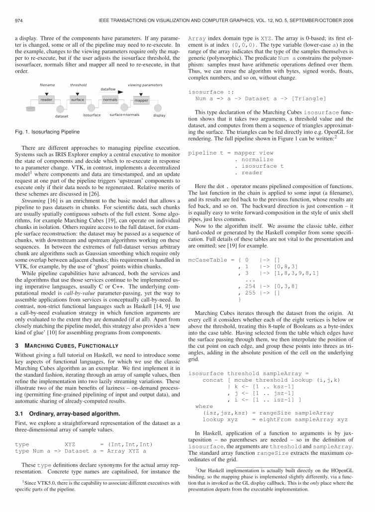
a display. Three of the components have parameters. If any parame-ter is changed, some or all of the pipeline may need to re-execute. Inthe example, changes to the viewing parameters require only the map-per to re-execute, but if the user adjusts the isosurface threshold, theisosurfacer, normals filter and mapper all need to re-execute, in thatorder.

Fig. 1. Isosurfacing Pipeline

There are different approaches to managing pipeline execution.Systems such as IRIS Explorer employ a central executive to monitorthe state of components and decide which to re-execute in responseto a parameter change. VTK, in contrast, implements a decentralizedmodel1 where components and data are timestamped, and an updaterequest at one part of the pipeline triggers ‘upstream’ components toexecute only if their data needs to be regenerated. Relative merits ofthese schemes are discussed in [26].

Streaming [16] is an enrichment to the basic model that allows apipeline to pass datasets in chunks. For scientific data, such chunksare usually spatially contiguous subsets of the full extent. Some algo-rithms, for example Marching Cubes [19], can operate on individualchunks in isolation. Others require access to the full dataset, for exam-ple surface reconstruction: the dataset may be passed as a sequence ofchunks, with downstream and upstream algorithms working on thesesequences. In between the extremes of full-dataset versus arbitrarychunk are algorithms such as Gaussian smoothing which require onlysome overlap between adjacent chunks; this requirement is handled inVTK, for example, by the use of ‘ghost’ points within chunks.

While pipeline capabilities have advanced, both the services andthe algorithms that use those services continue to be implemented us-ing imperative languages, usually C or C++. The underlying com-putational model is call-by-value parameter-passing, yet the way toassemble applications from services is conceptually call-by-need. Incontrast, non-strict functional languages such as Haskell [14, 9] usea call-by-need evaluation strategy in which function arguments areonly evaluated to the extent they are demanded (if at all). Apart fromclosely matching the pipeline model, this strategy also provides a ‘newkind of glue’ [10] for assembling programs from components.

3 MARCHING CUBES, FUNCTIONALLY

Without giving a full tutorial on Haskell, we need to introduce somekey aspects of functional languages, for which we use the classicMarching Cubes algorithm as an exemplar. We first implement it inthe standard fashion, iterating through an array of sample values, thenrefine the implementation into two lazily streaming variations. Theseillustrate two of the main benefits of laziness – on-demand process-ing (permitting fine-grained pipelining of input and output data), andautomatic sharing of already-computed results.

3.1 Ordinary, array-based algorithm.

First, we explore a straightforward representation of the dataset as athree-dimensional array of sample values.

type XYZ = (Int,Int,Int)

type Num a => Dataset a = Array XYZ a

These type definitions declare synonyms for the actual array rep-resentation. Concrete type names are capitalised, for instance the

1Since VTK5.0, there is the capability to associate different executives with

specific parts of the pipeline.

Array index domain type is XYZ. The array is 0-based; its first el-ement is at index (0,0,0). The type variable (lower-case a) in therange of the array indicates that the type of the samples themselves isgeneric (polymorphic). The predicate Num a constrains the polymor-phism: samples must have arithmetic operations defined over them.Thus, we can reuse the algorithm with bytes, signed words, floats,complex numbers, and so on, without change.

isosurface ::

Num a => a -> Dataset a -> [Triangle]

This type declaration of the Marching Cubes isosurface func-tion shows that it takes two arguments, a threshold value and thedataset, and computes from them a sequence of triangles approximat-ing the surface. The triangles can be fed directly into e.g. OpenGL forrendering. The full pipeline shown in Figure 1 can be written:2

pipeline t = mapper view

. normalize

. isosurface t

. reader

Here the dot . operator means pipelined composition of functions.The last function in the chain is applied to some input (a filename),and its results are fed back to the previous function, whose results arefed back, and so on. The backward direction is just convention – itis equally easy to write forward-composition in the style of unix shellpipes, just less common.

Now to the algorithm itself. We assume the classic table, eitherhard-coded or generated by the Haskell compiler from some specifi-cation. Full details of these tables are not vital to the presentation andare omitted; see [19] for example.

mcCaseTable = { 0 |-> []

, 1 |-> [0,8,3]

, 3 |-> [1,8,3,9,8,1]

...

, 254 |-> [0,3,8]

, 255 |-> []

}

Marching Cubes iterates through the dataset from the origin. Atevery cell it considers whether each of the eight vertices is below orabove the threshold, treating this 8-tuple of Booleans as a byte-indexinto the case table. Having selected from the table which edges havethe surface passing through them, we then interpolate the position ofthe cut point on each edge, and group these points into threes as tri-angles, adding in the absolute position of the cell on the underlyinggrid.

isosurface threshold sampleArray =

concat [ mcube threshold lookup (i,j,k)

| k <- [1 .. ksz-1]

, j <- [1 .. jsz-1]

, i <- [1 .. isz-1] ]

where

(isz,jsz,ksz) = rangeSize sampleArray

lookup xyz = eightFrom sampleArray xyz

In Haskell, application of a function to arguments is by jux-taposition – no parentheses are needed – so in the definition ofisosurface, the arguments are threshold and sampleArray.The standard array function rangeSize extracts the maximum co-ordinates of the grid.

2Our Haskell implementation is actually built directly on the HOpenGL

binding, so the mapping phase is implemented slightly differently, via a func-

tion that is invoked as the GL display callback. This is the only place where the

presentation departs from the executable implementation.

974

DUKE et al.: FINE-GRAINED VISUALIZATION PIPELINES

The larger expression in square brackets is a list comprehension3,and denotes the sequence of all applications of the function mcube

to some arguments, where the variables (i,j,k) range over (or aredrawn from) the given enumerations. The enumerators are separatedfrom the main expression by a vertical bar, and the evaluation ordercauses the final variable i to vary most rapidly. This detail is of interestmainly to ensure good cache behaviour, if the array is stored with x-dimension first. The comprehension can be viewed as equivalent tonested loops in imperative languages.

The result of computing mcube over any single cell is a sequenceof triangles. These per-cube sequences are concatenated into a singleglobal sequence, by the standard function concat.

Now we look more closely at the data structure representing an in-dividual cell. For a regular cubic grid, this is just an 8-tuple of valuesfrom the full array.

type Cell a = (a,a,a,a,a,a,a,a)

eightFrom :: Array XYZ a -> XYZ -> Cell a

eightFrom arr (x,y,z) =

( arr!(x,y,z), arr!(x+1,y,z)

, arr!(x+1,y+1,z), arr!(x,y+1,z)

, arr!(x,y,z+1), arr!(x+1,y,z+1)

, arr!(x+1,y+1,z+1), arr!(x,y+1,z+1)

)

Next, we need to introduce higher-order functions. From the veryname “functional language” one can surely guess that functions areimportant. Indeed, passing functions as arguments, and receivingfunctions as results, comes entirely naturally. A function that receivesor returns a function is called higher-order. We have seen two ex-amples thus far: mcube’s second argument is the function lookup,but also, the composition operator . is just a higher-order functionas well. Since this operator is the essence of the pipeline model, let’slook briefly at its definition:

(.) :: (b->c) -> (a->b) -> a -> c

(f . g) x = f (g x)

Dot takes two functions as arguments, with a third argument beingthe initial data. The result of applying the second function to the datais used as the argument to the first function. The type signature shouldhelp to make this clear - each type variable, a, b, and c, stands forany arbitrary (polymorphic) type, where for instance each occurrenceof a must be the same, but a and b may be different. Longer chainsof these compositions can be built up, as we have already seen in theearlier definition of pipeline.

Shortly, we will need another common higher-order function, map,which takes a function f and applies it to every element of a sequence:

map :: (a->b) -> [a] -> [b]

map f [] = []

map f (x:xs) = f x : map f xs

This definition uses pattern-matching to distinguish the empty se-quence [], from a non-empty sequence whose initial element is x,with the remainder of the sequence denoted by xs. Colon : is usedboth in pattern-matching, and to construct a new list.

Finally, to the definition of mcube:

mcube :: a -> (XYZ->Cell a) -> XYZ

-> [Triangle]

mcube th lookup (x,y,z) =

group3 (map (interpolate th cell (x,y,z))

(mcCaseTable ! bools))

where

cell = lookup (x,y,z)

bools = toByte (map8 (>th) cell)

3It bears similarities to Zermelo-Frankel (ZF) set comprehensions in math-

ematics.

group3 :: [a] -> [(a,a,a)]

group3 (x:y:z:ps) = (x,y,z):group3 ps

group3 [] = []

The cell of vertex sample values is found using the lookup

function that has been passed in. We derive an 8-tuple of booleansby comparing each sample with the threshold (map8 is a higher-orderfunction like map, only over a fixed-size tuple rather than an arbitrarysequence), then convert the 8 booleans to a byte (bools) to index intothe classic case table (mcCaseTable).

The result of indexing the table is the sequence of edges cut bythe surface. Using map, we perform the interpolation calculation forevery one of those edges, and finally group those interpolated pointsinto triples as the vertices of triangles to be rendered; group3 is usedagain in later steps, and hence is defined globally. The linear interpo-lation is standard:

interpolate :: Num a => a -> Cell a -> XYZ

-> Edge

-> TriangleVertex

interpolate thresh cell (x,y,z) edge =

case edge of

0 -> (x+interp, y, z)

1 -> (x+1, y+interp, z)

...

11 -> (x, y+1, z+interp)

where

interp = (thresh - a) / (b - a)

(a,b) = selectEdgeVertices edge cell

Although interpolate takes four arguments, it was initiallyapplied to only three in mcube. This illustrates another importanthigher-order technique: a function of n arguments can be partially ap-plied to its first k arguments; the result is a specialised function of n−karguments, with the already-supplied values ‘frozen in’.

3.2 Observations.

The implementation outlined so far is naive in several respects: (1)The entire dataset is needed in memory before we can begin any pro-cessing. (2) The work of comparing a vertex to the threshold valueis repeated eight times, once for every cell it adjoins. (3) The workof interpolating along an edge is repeated if we revisit the same edgeagain within that cell. (4) The same interpolation calculation is re-peated again when we visit the three neighbouring cells that share thesame edge. The following sections address these issues in turn.

3.3 Streaming the dataset on-demand.

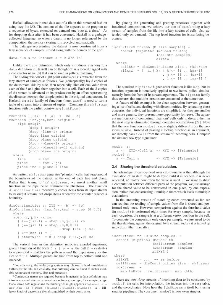
The monolithic array data structure implies that the entire dataset isin memory simultaneously, yet the algorithm only ever needs a smallportion of the dataset. At any one moment, a single point and 7 ofits neighbours suffices, making up a unit cube of sample values. If wecompare this with a typical array or file storage format for regular grids(essentially a linear sequence of samples), then the unit cube is entirelycontained within a “window” of the file, corresponding to exactly oneplane + line + sample of the volume. The ideal solution is to slide thiswindow over the file, constructing one unit cube on each iteration, anddropping the previous unit cube. Figure 2 illustrates the idea.

Fig. 2. Sliding a window over a grid

975


Haskell allows us to read data out of a file in this streamed fashionusing lazy file I/O. The content of the file appears to the program asa sequence of bytes, extended on-demand one byte at a time.4 Asfor dropping data after it has been consumed, Haskell is a garbage-collected language, so when a datum is no longer referenced by thecomputation, the memory storing it is recycled automatically.

The datatype representing the dataset is now constructed from alazy sequence of samples, stored along with the bounds of the grid:

data Num a => Dataset a = D XYZ [a]

Unlike the type definition, which only introduces a synonym, adata definition in Haskell can be thought of as a record, tagged witha constructor name (D) that can be used in pattern matching.5

The sliding window of eight point values (cell) is extracted from thelazy stream of samples as follows. We (conceptually) lay 8 copies ofthe datastream side-by-side, then repeatedly slice off one value fromeach of the 8 and glue them together into a cell. Each of the 8 copiesof the stream is advanced on its predecessor by an offset representingthe distance between the sample points in the original data stream. InHaskell, the zip family of functions (here, zip8) is used to turn atuple-of-streams into a stream-of-tuples. (Compare this mkStreamfunction with the earlier point-wise eightFrom.)

mkStream :: XYZ -> [a] -> [Cell a]

mkStream (isz,jsz,ksz) origin =

zip8 origin

(drop 1 origin)

(drop (line+1) origin)

(drop line origin)

(drop plane origin)

(drop (plane+1) origin)

(drop (planeline+1) origin)

(drop planeline origin)

where

line = isz

plane = isz * jsz

planeline = plane + line

As written, mkStream generates ‘phantom’ cells that wrap aroundthe boundaries of the dataset, at the end of each line and plane.Rather than trying to ‘fix’ mkStream, we insert another smallfunction in the pipeline to eliminate the phantoms. The functiondisContinuities recursively copies items from its input streamto its output stream, but drops items whenever the counter reaches aboundary.

disContinuities :: XYZ -> [b] -> [b]

disContinuities (isz,jsz,ksz) = step (0,0,0)

where

step (i,j,k) (x:xs)

| i==(isz-1) = step (0,j+1,k) xs

| j==(jsz-1) = step (0,0,k+1)

(drop (isz-1) xs)

| k==(ksz-1) = []

| otherwise = x : step (i+1,j,k) xs

The vertical bars in this definition introduce guarded equations;given a function of the form f a | p = e, the call f v evaluatesto e provided v matches the pattern a and the expression p evalu-ates to True. Multiple guards are tried from top to bottom until onesucceeds.

4For efficiency, the underlying system may choose to hold variable-size

buffers for the file, but crucially, that buffering can be tuned to match avail-

able resources of memory, disc, and processor.5Constructor names are required because in general, a data definition may

introduce several alternative constructors for a given type; for example, a type

that allowed both regular and rectilinear grids might appear as Dataset a =

Reg XYZ [a] | Rect ([Float],[Float],[Float]) [a]. Dif-

ferent kinds of dataset are then distinguished by their constructor.

By glueing the generating and pruning processes together withfunctional composition, we achieve our aim of transforming a lazystream of samples from the file into a lazy stream of cells, also ex-tended only on demand. The top-level function for isosurfacing be-comes:

isosurfaceS thresh (D size samples) =

concat (zipWith2 (mcubeS thresh)

(cellStr samples)

allXYZ )

where

cellStr = disContinuities size . mkStream

allXYZ = [ (i,j,k) | k <- [1 .. ksz-1]

, j <- [1 .. jsz-1]

, i <- [1 .. isz-1] ]

The standard zipWith2 higher-order function is like map, but itsfunction argument is iteratively applied to two items, pulled simulta-neously from the front of its stream arguments. The zipWith familythus ensures that multiple streams are consumed at the same rate.

A feature of this example is the clean separation between generat-ing a list of cells, and dealing with discontinuities. By separating theseconcerns, the individual functions are simplified. As they are smallerand more generic, they present more opportunity for reuse. The appar-ent inefficiency of computing ‘phantom’ cells only to discard them inthe next step is eliminated through compiler optimization [27]. Notethat the new function mcubeS is now slightly different from the pre-vious mcube. Instead of passing a lookup function as an argument,we directly pass a cell from the stream of incoming cells. Comparethe old and new type signatures:

mcube ::

a -> (XYZ->Cell a) -> XYZ -> [Triangle]

mcubeS ::

a -> Cell a -> XYZ -> [Triangle]

3.4 Sharing the threshold calculation.

The advantage of call-by-need over call-by-name is that although theevaluation of an item might be delayed until it is needed, it is neverrepeated, no matter how often the value is used. If we want to sharea computation between different parts of the program, we just arrangefor the shared value to be constructed in one place, by one expres-sion, rather than constructing it multiple times which leads to multipleevaluations.

In the streaming version of marching cubes presented so far, wecan see that the reading of sample values from file is shared and per-formed only once. However, comparison against the threshold value(in mcubeS) is performed eight times for every sample, because oneach occasion, the sample is at a different vertex position in the cell.To compute the comparison only once per sample, we just need to dothe thresholding against the original byte stream, before it is tupled upinto cells, rather than after.

isosurfaceT th (D size samples) =

concat (zipWith3 (mcubeT th)

(cellStream samples)

(idxStream samples)

allXYZ )

where

allXYZ = ... -- as before

cellStream = disContinuities size . mkStream

idxStream =

map toByte . cellStream . map (>th)

There are now three streams of incoming data to be consumed bymcubeT: the cells for interpolation, the indexes into the case table,and the co-ordinates. Note how the idxStream is itself built usingsmaller pipelines. The consumer mcubeT is now even simpler:

976


mcubeT :: a -> Cell a -> Byte -> XYZ

-> [Triangle]

mcubeT th cell index (x,y,z) =

group3 (map (interpolate th cell (x,y,z))

(mcCaseTable ! index))

3.5 Sharing the edge interpolation calculation.

Taking the notion of sharing-by-construction one step further, we nowmemoize the interpolation of edges. Recall that, in the result of themcCaseTable, the sequence of edges through which the isosurfacepasses may have repeats, because the same edge belongs to more thanone triangle of the approximated surface.

But in general, an edge that is incident on the isosurface is also com-mon to four separate cells, and we would like to share the interpolationcalculation with those cells too. So, just as the threshold calculationwas performed at an outer level, on the original datastream, we can dosomething similar here.

Instead of an 8-tuple of vertices, we build a 12-tuple of possibleedges. Before looking up the case table in mcubeI, we cannot knowwhich of those edges are actually incident on the surface. But that doesnot matter – we describe how to calculate the interpolation on all 12edges, safe in the knowledge that each result will only be computed ifthat edge is actually needed!

type CellEdge a = (a,a,a,a,a,a,a,a,a,a,a,a)

mkCellEdges :: a -> XYZ -> [a] -> [CellEdge a]

mkCellEdges thresh (isz,jsz,ksz) stream =

zip12 inter_x

(drop line inter_x)

(drop plane inter_x)

(drop (plane+line) inter_x)

inter_y

(drop 1 inter_y)

(drop plane inter_y)

(drop (plane+1) inter_y)

inter_z

(drop 1 inter_z)

(drop line inter_z)

(drop (line+1) inter_z)

where

line = isz

plane = isz*jsz

offset d = zipWith2 interpolate

stream

d

inter_x = offset (drop 1 stream)

inter_y = offset (drop line stream)

inter_z = offset (drop plane stream)

interpolate v0 v1 = (thresh-v0) / (v1-v0)

Here, the datastream is offset in each of the x, y, and z dimensions,zipped with the original copy, and the interpolation calculated pairwisein each dimension. The three dimensions are then zipped together,taking four edges from each, to make up each cell.

isosurfaceI th (D size samples) =

concat (zipWith3 mcubeI

(edgeStream samples)

(idxStream samples)

allXYZ )

where

edgeStream = disContinuities size

. mkCellEdges th size

... -- idxStream, allXYZ as before

Finally, mcubeI does no interpolation itself, it merely selectsalready-interpolated values from the CellEdge structure and addsthe absolute grid position.

mcubeI :: CellEdge a -> Byte -> XYZ

-> [Triangle]

mcubeI edges index (x,y,z) =

group3 (map (selectEdge edges (x,y,z))

(mcCaseTable ! index))

4 UNAMBIGUOUS MARCHING CUBES

It is well-known that in the original marching cubes, ambiguous casescan occur, and the original method has been enhanced and general-ized in various ways to assure topological correctness of the result.Chernyaev [4] proposed a definitive classification of all the ambiguouscases. Lewiner et.al. [18] completed the resolution of internal ambi-guities, and defined a method, ‘MC33’, guaranteed to yield a manifoldsurface with no cracks between or within cubes. Although MC33 re-quires a more extensive set of test/case tables than the original algo-rithm, changes to the top level structure of the functional implemen-tation are surprisingly small; at the top level, we have simply added,as a fourth stream, the original cells of samples (used to resolve ambi-guities), to the streams of ready-interpolated edges, case-table indicesand grid positions. Compare the following with isosurfaceT andisosurfaceI:

isosurfaceU thresh (D size samples) =

concat (zipWith4 (mcubeU thresh)

(edgeStream samples)

(idxStream samples)

(cellStream samples)

allXYZ )

where

... -- cellStream etc. just as before

The mcubeU function differs from mcubeT in only two ways. (1)It uses a different two-stage case-table to look up the edges incidenton the surface, of which the tiling stage occasionally needs the originalsample cell to test for face-cracks. (2) The edges returned now in-clude a distinguished marker to signal the need for tri-linear interpola-tion to resolve internal ambiguity. A simple auxiliary function detectsthe marker, or otherwise just picks the corresponding edge from theedge stream.

mcubeU :: a -> CellEdge a -> Byte -> Cell a

-> XYZ -> [Triangle]

mcubeU thresh edges index cell (x,y,z) =

group3 (map (select (x,y,z))

cases)

where

cases =

mc33tiles cell (mc33CaseTable ! index)

select idx 12 =

triInterpolate idx cell thresh

select idx _ = selectEdge edges idx

5 RESULTS AND EVALUATION

Figures 3 and 4 show the ‘fuel’ and ‘neghip’ datasets, surfaced usingour functional implementation. Triangles are coloured as a function ofthe point within the output stream at which they arrive, and the figuresthus show how the streaming implementation progresses through thedataset (compare with Figure 2). In the remainder of this section thefunctional approach is evaluated against three criteria: time and spaceperformance, requirements for data streaming [16], and the issue ofclarity and economy of expression.

5.1 Time and Space Profiles

Performance numbers are given for the initial array-based version, andan optimised streaming version of marching cubes written in Haskell,over a range of sizes of dataset (all taken from volvis.org), andcompared with VTK 5’s marching cubes implementation in C++.The relevant characteristics of the datasets are summarised in Ta-ble 1, where the streaming window size is calculated in bytes as one

977


Fig. 3. Functionally surfaced dataset coloured to show age of triangles in stream.

Fig. 4. Streamed dataset, colour mapped to stream position.

Table 1. Dataset Statistics.dataset size input (b) window (b) surface (v)

silicium (98,34,34) 113,288 3,431 103,020neghip (64,64,64) 262,144 4,161 131,634hydrogen (128,128,128) 2,097,152 16,513 134,952lobster (301,324,56) 5,461,344 97,826 1,373,196engine (256,256,128) 8,388,608 65,793 1,785,720statueLeg (341,341,93) 10,814,133 116,623 553,554aneurism (256,256,256) 16,777,216 65,793 1,098,582skull (256,256,256) 16,777,216 65,793 18,415,053stent8 (512,512,174) 45,613,056 262,657 8,082,312vertebra8 (512,512,512) 134,217,728 262,657 197,497,908

plane+line+1, and the size of the extracted surface is measured in ver-tices.

Table 2 gives the absolute time taken to compute an isosurface atthreshold value 20 for every dataset, on a 2.3GHz Macintosh G5 with2Gb of memory, compiled with the ghc compiler and -O2 optimiza-tion. We also normalise time against dataset size, giving the averagenumber of microseconds expended per sample.

Table 3 shows the peak live memory usage of each version of thealgorithm, as determined by heap profiling. Again, we normalise theabsolute numbers against the size of the dataset required in memoryat any one time. For the VTK and array-based versions, this is theentire dataset, whilst for the streaming version, it is the (much smaller)window size.

The time performance in Haskell (both array-based and streamingversions) scales linearly with the size of dataset. It can also be seenthat the memory performance is exactly proportional to the size ofthe input (array) or sliding window (streaming). In contrast, the VTKresults, both time and memory, are more proportionally weighted tothe size of the output surface, than the input.

Although for smaller datasets, our current speeds do not comparewell with VTK, the clear and readable specification of the algorithmswas our main aim. Elegant Haskell is not necessarily efficient Haskell!But, due to referential transparency and equational reasoning, it is pos-sible to apply formal transformations that preserve the code’s seman-tics whilst improving its runtime performance. Some improvement

Table 2. Time Performancetime (s) (μs/sample)

dataset array stream VTK arr str VTK

silicium 0.626 0.386 0.19 5.53 3.40 1.67neghip 1.088 0.852 0.29 4.15 3.25 1.11hydrogen 8.638 6.694 0.51 4.12 3.19 0.24lobster 25.37 18.42 5.69 4.65 3.37 1.04engine 44.51 28.06 5.29 5.31 3.35 0.63statueLeg 48.78 34.54 2.78 4.51 3.19 0.25aneurism 72.98 54.44 5.69 4.35 3.24 0.33skull 79.50 57.19 79.03 4.74 3.41 4.71stent8 287.5 154.9 33.17 6.30 3.40 0.73vertebra8 703.0 517.1 755.0 5.24 3.85 5.62

techniques that achieve speeds within 2-3× of C code, may currentlybe applied manually [8, 2], whilst research continues in generalizingsimilar transformations to be applied automatically during the opti-mization stage of the compiler [27]. This approach promises (eventu-ally) to allow elegance to co-exist with efficiency.

Even without these possible performance improvements, it is clearthat the ability to stream datasets in a natural fashion makes the func-tional approach much more scalable to larger problem sets. For in-stance, the streaming Haskell version is actually faster than VTK forthe larger surfaces generated by skull and vertebra8. We speculate thatwhere other toolkits might eventually need to swap to a different out-of-core algorithm, the streaming approach will just continue to work.

5.2 Visualization Criteria

Compare the properties of our fine-grained streaming approach withthe requirements for data streaming set out in [16].

Caching is achieved by coupling streamed data access (sec 3.3) withmemoization (sec 3.5) of results.

Demand-Driven computation is a natural product of call-by-needevaluation (Section 3.4). Shared sub-expressions are evaluated at mostonce, e.g. the bi-linear interpolant of a given edge is computed onlyif needed (sec 3.4). Incoming data is transformed only to the extentthat it contributes to the growing surface mesh, and grid memory that‘falls off’ the back of the window is recycled automatically. By mem-

978


Table 3. Memory Usage

memory (MB) (bytes/residency)dataset array stream VTK array stream VTK

silicium 0.120 0.120 1.1 1.06 35.0 9.71neghip 0.270 0.142 1.4 1.03 34.1 5.34hydrogen 2.10 0.550 3.0 1.00 33.3 1.43lobster 5.45 3.10 19.5 1.00 31.7 3.57engine 8.25 2.10 25.4 0.98 31.9 3.03statueLeg 11.0 3.72 15.9 1.02 31.9 1.47aneurism 17.0 2.10 28.1 1.01 31.9 1.67skull 17.0 2.13 185.3 1.01 32.4 11.04stent8 46.0 8.35 119.1 1.01 31.8 2.61vertebra8 137.0 8.35 1,300.9 1.02 31.8 9.69

oization, we extend laziness to wider sharing of computations, e.g.avoiding recomputing the edge interpolant for each neighbouring cell(sec 3.5).

Hardware architecture independence is supported in two ways.Through polymorphic types (sec 3.1) functions can be defined inde-pendent of the datatypes available on a specific architecture; type pred-icates (e.g. ‘Num a’) allow developers to set out the minimum require-ments that particular types must satisfy. Beyond the scope of this pa-per, polytypism [13], also known as structural polymorphism on types,has the capability to abstract over data organisation and traversal, e.g.a polytypic marching cubes could be applied to other kinds of datasetorganization like irregular grids.

Component Based development, as highlighted throughout Section 3,is fundamental to functional programming [10]. In [16], ‘components’are coarse-grained modules encapsulating visualization algorithms; inthis paper we have shown that component-based assembly can bemuch finer-grained. For example, the streaming operators would bejust as applicable in the implementation of flow algorithms, generat-ing streamlines. Functional building blocks, in the form of combinatorlibraries, have been developed for a range of problems, e.g. pretty-printing [11], XML transformation [29], and circuit layout [1]. Therich type systems found in functional languages aid in program de-velopment; higher-order types exactly describe how components maybe safely plugged together. The assembly of functional abstractionsfrom smaller units has a similar feeling to pipeline assembly [26], butapplies across all levels of abstraction.

5.3 Clarity

In the quest for faster, more space-efficient algorithms, other quali-ties required of visualization systems are easily overlooked. Law et.al.briefly discuss other software design properties like robustness and ex-tensibility. But when pictures inform us on critical issues as diverse assurgical procedure, storm forecasting and long-term decision-makinglinked to climate change, we should add the over-riding criterion thatalgorithms must be evidently correct.

Assurance of correctness is aided in functional programming bythree means. (1) Strong static polymorphic type systems, and auto-matic memory management, eliminate entire classes of errors that areotherwise commonplace in imperative languages. (2) Conciseness ofexpression means that it is possible for a reader to understand moreof the big picture at once. (This paper contains the majority of themarching cubes code – the complete program beyond the classic tableis about 200 lines.) (3) As there are no ‘side-effects’, expressions canbe manipulated using the kind of equational reasoning familiar frommathematics.

6 RELATED WORK

While call-by-need is implicit in lazy functional languages, severalefforts have explored more ad hoc provision of lazy evaluation in im-perative implementations of visualization systems. Moran et al. [21]exploit lazy evaluation for working with large time-series datasets ina visualization system based on the Demand Driven Visualizer (DDV)

calculator paradigm for computation and visualization of large fields.In their system derived fields quantities are evaluated either on demand(lazy evaluation), as a whole field (eager evaluation), or via a cache oflazily evaluated results (lazy but thrifty evaluation).

Lazy evaluation has also been used in several visualization systems.The Unsteady Flow Analysis Toolkit (UFAT) [15] allows users to com-pute field values on demand. Cox et.al. [5] modified UFAT to supportdemand-driven loading of data into main memory, achieving good per-formance in the visualization of large computational fluid dynamicsdata sets. More generally, in the demand-driven (‘pull-model’) sys-tems noted in Section 2, e.g. VTK [26] and SCIRun [25], laziness un-derpins a streaming interface; modules can request just the data neededfrom upstreams modules within given spatial extents, and operationsto produce these data are executed only on demand.

Isenburg et.al. [12] propose a streaming mesh format for polygo-nal meshes and discuss techniques to construct streamed meshes. Inthis approach mesh elements (faces and vertices) appear interleavedin the stream, and finalization tags record when a vertex is last ref-erenced. Finalized vertices are guaranteed not to be accessed further,and can thus be removed from main memory, an ad hoc form of thegeneral garbage collection techniques provided by the Haskell run-time system. Laziness is achieved by introducing vertices only whenneeded, but at the cost of re-organizing the entire file data-structureto generate a proper data layout in terms of vertices and faces order-ing. The authors propose an application of their streaming approachto isosurface extraction techniques, and show the benefits gained fromstreamed inputs; but the advantage is limited to cases where the vol-ume data changes often and only few isosurface values are evaluated.

When data are generated by computationally intense simulationsand multiple isosurfaces are generated to explore the dataset, the tech-nique of Mascarenhas et.al. [20] is more suitable. Adopting a contourfollowing approach, their method uses sparse traversal to avoid com-putation at each grid location. Coupled with lazy evaluation of databased on a streamed format, performance is reported as faster than ex-emplar eager systems (as in [21]). As shown by Chandrasekaran et.al.[3] a lazy approach improves the throughput of an application: from auser’s point of view, first results are returned quickly; from the appli-cation point of view, often only a portion of the result set is actuallyneeded.

7 CONCLUSION

The purely functional streaming implementation of marching cubesdeveloped in this paper demonstrates significant space savings com-pared with an approach based on monolithic datasets. This is not initself surprising, given prior work on streaming, but shows that ele-gance and clarity need not be sacrificed to meet certain performancecriteria. Streaming within visualization occupies an important nichebetween fully in-core and fully out-of-core methods. A feature of thefunctional approach is that data is pulled off-disk as needed, withoutthe programmer resorting to explicit control over buffering. Data isretained in memory only as long as required: in our case a sample isheld while plane + line + 1 cells are processed, and discarded auto-matically.

Motivated by the demands of large-scale data, visualization re-searchers have explored techniques for lazy and demand-driven eval-uation. But deployment of these techniques has been limited by theneed to access these services from within an imperative programmingsystem. We have shown how a programming technology based funda-mentally on lazy evaluation allows the use of streaming, call-by-need,and memoization at a fine level of granularity. Functional forms fortraversal and computation can be reused across different algorithms; insurface extraction for example, the sliding window used here is appli-cable to sweep-based seed-set generation. We are currently exploringuse of generic programming techniques to extend the work to othertypes of grid (e.g. tetrahedral meshes and unstructured datasets), andto other surface extraction methods. The result should be a small setof combinators from which specific traversal and surfacing tools canbe constructed.

979


Source Material: All programs used in the paper are available from:http://hackage.haskell.org/trac/PolyFunViz/

ACKNOWLEDGEMENTS

The work reported in this paper was funded by the UK Engineeringand Physical Sciences Research Council.

REFERENCES

[1] P. Bjesse, K. Claessen, M. Sheeran, and S. Singh. Lava: Hardware de-

sign in haskell. In International Conference on Functional Programming,

pages 174–184, 1998.

[2] M. Chakravarty and G. Keller. An approach to fast arrays in haskell. In

Advanced Functional Programming 2002, number 2638 in Lecture notes

in Computer Science, pages 27–58. Springer-Verlag, 2003.

[3] S. Chandrasekaran and M. Franklin. PSoup: a system for streaming

queries over streaming data. VLDB Journal, 12(2):140–156, 2003.

[4] E. Chernyaev. Marching cubes 33: Construction of topologically correct

isosurfaces. Technical Report Technical Report CERN CN 95-17, CERN,

1995.

[5] M. Cox and D. Ellsworth. Application-controlled demand paging for out-

of-core visualization. In Proceedings of Visualization ’97, pages 235–ff.

IEEE Computer Society Press, 1997.

[6] R. Haber and D. McNabb. Visualization idioms: A conceptual model for

scientific visualization systems. In Visualization in Scientific Computing.

IEEE Computer Society Press, 1990.

[7] P. Haeberli. ConMan: a visual programming language for interactive

graphics. In Proceedings of SIGGRAPH’88, pages 103–111. ACM Press,

1988.

[8] P. H. Hartel et. al. Benchmarking implementations of functional lan-

guages with pseudoknot, a float-intensive benchmark. Journal of Func-

tional Programming, 6(4):621–656, 1996.

[9] Haskell: A purely functional language. http://www.haskell.org, Last vis-

ited 27-03-2006.

[10] J. Hughes. Why functional programming matters.

Computer Journal, 32(2):98–107, 1989. See also

http://www.cs.chalmers.se/ rjmh/Papers/whyfp.html.

[11] J. Hughes. The design of a pretty-printing library. In J. Jeuring and

E. Meijer., editors, Advanced Functional Programming, volume 925.

Springer Verlag, 1995.

[12] M. Isenburg and P. Lindstrom. Streaming meshes. In Proceedings of

Visualization’05, page 30, 2005.

[13] J. Jeuring and P. Jansson. Polytypic programming. In J. Launchbury,

E. Meijer, and T. Sheard, editors, Tutorial Text 2nd Int. School on Ad-

vanced Functional Programming, Olympia, WA, USA, 26–30 Aug 1996,

volume 1129, pages 68–114. Springer-Verlag, 1996.

[14] S. P. Jones, editor. Haskell’98 Language and Libraries: The Revised

Report. Cambridge University Press, 2003.

[15] D. Lane. UFAT: a particle tracer for time-dependent flow fields. In Pro-

ceedings of Visualization ’94, pages 257–264. IEEE Computer Society

Press, 1994.

[16] C. Law, W. Schroeder, K. Martin, and J. Temkin. A multi-threaded

streaming pipeline architecture for large structured data sets. In Proceed-

ings of Visualization ’99, pages 225–232. IEEE Computer Society Press,

1999.

[17] M. Levoy. Spreadsheets for images. Computer Graphics, 28(Proceedings

of SIGGRAPH’94):139–146, 1994.

[18] T. Lewiner, H. Lopes, A. Vieira, and G. Tavares. Efficient implementa-

tion of marching cubes’ cases with topological guarantees. Journal of

Graphics Tools, 8(2):1–15, 2003.

[19] W. Lorensen and H. Cline. Marching cubes: A high resolution 3d surface

construction algorithm. In Proceedings of SIGGRAPH’87, pages 163–

169. ACM Press, 1987.

[20] A. Mascarenhas, M. Isenburg, V. Pascucci, and J. Snoeyink. Encoding

volumetric grids for streaming isosurface extraction. In 3DPVT, pages

665–672, 2004.

[21] P. Moran and C. Henze. Large field visualization with demand-driven cal-

culation. In Proceedings of Visualization’99, pages 27–33. IEEE Com-

puter Society Press, 1999.

[22] D. Nadeau. Volume scene graphs. In Proceedings of the Symposium on

Volume Visualization, pages 49–56. ACM Press, 2000.

[23] C. North and B. Shneiderman. Snap-together visualization: a user inter-

face for coordinating visualizations via relational schemata. In AVI’00:

Proceedings of Advanced Visual Interfaces, pages 128–135. ACM Press,

2000.

[24] A. Pang and K. Smith. Spray rendering: visualization using smart parti-

cles. In G. Nielson and R. Bergeron, editors, Proceedings of Visualiza-

tion’93, pages 283–290. IEEE Computer Society Press, 1993.

[25] S. Parker, D. Weinstein, and C. Johnson. The SCIRun computational

steering software system. In Modern software tools for scientific comput-

ing, pages 5–44. Birkhauser Boston Inc., 1997.

[26] W. Schroeder, K. Martin, and B. Lorensen. The Visualization Toolkit: An

Object-Oriented Approach to 3D Graphics. Prentice Hall, second edition,

1998.

[27] J. Svenningsson. Shortcut fusion for accumulating parameters & zip-like

functions. In ICFP ’02: Proc. of International Conference on Functional

Programming, pages 124–132. ACM Press, 2002.

[28] C. Upson, T. Faulhaber Jr, D. Kamins, D. Laidlaw, D. Schlegel, J. Vroom,

and A. van Dam. The application visualization system: A computational

environment for scientific visualization. Computer Graphics and Appli-

cations, 9(4):30–42, 1989.

[29] M. Wallace and C. Runciman. Haskell and XML: Generic combinators

or type-based translation? In Proceedings of the Fourth ACM SIGPLAN

International Conference on Functional Programming (ICFP‘99), pages

148–159. ACM Press, 1999.

980

Fine-grained Visualization Pipelines and Lazy Functional Languages

Documents

Transcript of Fine-grained Visualization Pipelines and Lazy Functional Languages