A new direction in hydrodynamic stability: Beyond eigenvalues

AD-A261 846

NASA Contractor Report 191411

ICASE Report No. 92-71

ICASEA NEW DIRECTION IN HYDRODYNAMIC STABILITY:BEYOND EIGENVALUES

Lloyd N. TrefethenAnne E. TrefethenSatish C. ReddyTobin A. Driscoll D T IC

ELECTE

NASA Contract No. NAS1-19480December 1992 .......

Institute for Computer Applications in Science and EngineeringNASA Langley Research CenterHampton, Virginia 23681-0001

Operated by the Universities Space Research Association

£TRIBu,._14 STATE1VtEM .¶

Approved fox public releasO

National Aeronautics andSpace Administration 93-05247Langley Research CenterHampton, Virginia 23665-5225 I 111111iii 111111 INl 11111 11 Il II Q

93 3 11 077

A NEW DIRECTION IN HYDRODYNAMIC STABILITY:BEYOND EIGENVALUES

Lloyd N. Trefethen', Annm E. Trcfcthcn2 . Satish C. Reddy, Tobin A. Driscollt

ABSTRACT

Fluid flows that are smooth at low speeds become unstable and then turbulent at higher

speeds. This phenomenon has traditionally been investigated by linearizing the equations

of flow and looking for unstable eigenvalues of the linearized p)robleml, but the results agree

poorly in many cases with experiments. Nevertheless, it has become clear in recent years

that linear effects play a central role in hydrodynamic instal)ility. A reconciliation of these

findings with the traditional analysis can be obtained by considering the "pseudospectra" of

the linearized problem, which reveal that small perturbations to the smooth flow in the form

of streamwise vortices may be amplified by factors on the order of 10' by a linear mechanism,

even though all the eigenmodes are stable. The same principles apply also to other problems

in the mathematical sciences that involve non-orthogonal eigenfunctions.

Accesion For

NTIS CRA&IDTIC TAB

DTIC 1;2T-5 Unannounced [lJustification ....... ........

By .............................

Dist; ibution I

Availability Codes

Avail and I orDist Special.0

'Department of Computer Science, Cornell University, Ithaca, NY 14853. Research was supported by

the National Aeronautics and Space Administration under NASA Contract No. NASI-19480 while the firstauthor was in residence at the Institute for Computer Applications in Science and Engineering (ICASE),NASA Langley Research Center, Hampton, VA 23681-0001.

2 Cornell Theory Center, Cornell University, Ithaca, NY 14853.'Courant Institute of Mathematical Sciences, New York University, 251 Mercer Street, New York, NY

10012.'Center for Applied Mathematics, Cornell University, Ithaca, NY 14853.

Contents

1. Introduction

2. Streamwise vortices and streaks

3. Spectra and pseudospectra

4. Resonance curves

5. Transient energy growth

6. Physically interesting pseudomodes

7. The inviscid limit

8. Destabilizing perturbations and secondary instability

9. Nonlinear bootstrapping and transition to turbulence

10. Conclusion

References and notes

iii

Trefethen, Trefethen, Reddy and Driscoll - 2

Introduction

A change of paradigm is taking place in the field of hydrodynamic stabil-

ity. This is the field devoted to the study of how laminar fluid flows become

unstable, the precursor to turbulence (1, 2). It is well known that turbulence

is an unsolved problem, but not so well known that despite the efforts of gen-

erations of applied mathematicians beginning with Stokes, Kelvin, Rayleigh,

and Reynolds a century ago, many of the presumably simpler phenomena of

hydrodynamic stability also remain ill-understood (3).

The traditional paradigm is eigenvalue analysis:

I. Linearize about the laminar solution;

II. Look for unstable eigenvalues of the linearized problem.

An "unstable eigenvalue" means an eigenvalue in the complex upper half-plane,

corresponding to an eigenmode of the linearized problem that grows exponen-

tially as a function of time t. It is natural to expect that a flow will behave

unstably if and only if there exists such a growing eigenmode, and over the

years a great deal of knowledge has been obtained about which flows possess

such modes, a distinction that depends on the geometry, the Reynolds number,

and sometimes other parameters.

For some flows, the predictions of eigenvalue analysis match laboratory ex-

periments. Examples are Rayleigh-1B3nard convection (a stationary fluid heated

from below) and Taylor-Couette flow (between a stationary outer and a rotating

inner cylinder). For other flows, the predictions of eigenvalue analysis fail to

match most experiments. In this article we consider the two most extensively

studied examples of this kind: (plane) Couette flow, the flow with a linear ve-

locity profile between two infinite flat plates moving parallel to one another,

and (plane) Poiseuille flow, the flow with a parabolic velocity profile between

two stationary plates (Fig. 1). Other examples where eigenvalue analysis fails

include pipe Poiseuille flow (in a cylindrical pipe) and, to a lesser degree, Blasius

boundary layer flow (near a flat wall).

For Poiseuille flow, eigenvalue analysis predicts a critical Reynolds number

(4) R = 5772.22 at which instability should first occur (5), but in the laboratory,

transition to turbulence is observed at Reynolds numbers as low as R - 1000 (6).


(a) Couette

(b) Poiseuille

Fig. 1. Velocity profiles for the two laminar flows considered in this article(independent of x and z). The geometry is an infinite 3D slab of viscousincompressible fluid bounded by parallel walls. The laminar solutions sat-isfy the Navier-Stokes equations for all Reynolds numbers R, but for higherR the flows are unstable and rapidly become turbulent.

For Couette flow, eigenvalue analysis predicts stability for all R, but transition

is observed for Reynolds numbers as low as R ; 350 (7). These anomalies of"subcritical transition to turbulence" have been recognized for many years, and

the explanation has usually been attributed to step I above. If linearization has

failed, the reasoning goes, one must look more closely at the nonlinear terms,

or perhaps linearize about a solution other than the laminar one (the theory of"secondary instability" (8, 9)).

Recently it has emerged, however, that the failure of eigenvalue analysis

may more justly be attributable to step II. It is a fact of linear algebra that

even if all of the eigenvalues of a linear system are distinct and lie well inside

the lower half-plane, inputs to that system may be amplified by arbitrarily large

factors if the eigenfunctions are not orthogonal. A matrix or operator whose

eigenfunctions are orthogonal is said to be normal (10, 11). The linear operators

that arise in the B6nard and Taylor-Couette problems are normal or close to

normal. By contrast Reddy, Schmid and Henningson discovered in 1990 that the

operators that arise in Poiseuille and Couette flow are in a sense exponentially

far from normal (12). At about the same time the startling discovery was made

by Gustavsson (13) and Henningson (14) and independently by Butler and

Farrell (15) that small perturbations to these flows may be amplified by factors

of many thousands, even when all the eigenvalues are in the lower half-plane.

The paper by Butler and Farrell is an important and elegant one. It discusses

many details omitted here, and together with a related more recent paper by


100 104 105 21x 105

(a ,i 106k .D ...... ...

2

trnitototruecisosreat1 100. Te aaloou pictur

s Os

0 R

For. Coutt flowmu looksibquamlitaielfimailar excDeptuthatithrens ino blnackze

Reddy il and w Henaso (1) itfomstenoudtion of theold pres ndxz ae ntmwork1)

Fig.iluse t f of tosn. The black region, has alppear

insmanye papersade bookst and cnorrspndsd opaamelfcterns forsiwhichuntbeeiemdseit(8.Tecontours defining theshde regions crepntofieamliainfactre newan

quantify th non-mod afic000 atisponsil th mayl R > .In the laows.(Arec

expanaition tof thisbplotc is givenrivted net section0.) The pnloousspibiltyufrmpi

fication of perturbatiosq pofsiscou flmows eyon-oDe a inea r mechanisms has

beednd rognized for a centuryi(nc orm)tbutfunttion of r hecen pdveoents wri wa

nkgn ithustrat the se mag toud of the black re gion hahu e.mpoar

untbeeigenmodes exist (18) Thucntoursdefiin theifiadeteionis posibe. Thewn

quantifh onrs mousdetal eincrepn ofnt amplifications htmyocri hs flows. (Apecs

expansition tof thisulotc is givenrvted net section0.) The pnloossibiictyrempi

ficton Cofuertubteifons lofoksos fulttvlowsila byep nonmoal linearmecihanism hasc

beend reonizd fornagsentr (192), btfousth fundtino the reetdvlpmeents itr was)

qunotif konta the n-moagnamplificainolve were hacurgntese.ws Aprcs


An essential feature of the amplification process of Fig. 2 is that it acts

upon 3D perturbations of the laminar flow field. In much of the theoretical

literature of hydrodynamic stability, attention has been restricted to 2D (x-y)

perturbations, and in particular, the well-known Orr-Sommerfeld equation is

an eigenvalue equation for 2D perturbations. A principal justification for this

restriction has been Squire's theorem of 1933, which asserts that if a flow has an

unstable 3D eigenmode for some R, then it has an unstable 2D eigenmode for

some lower value of R (24). The new results indicate that this emphasis on 2D

perturbations has been misplaced. When only 2D perturbations are considered,

amplification is still possible, but far weaker.

This emphasis on 3D, linear but non-modal effects is the emerging new

paradigm in hydrodynamic stability.

Streamwise vortices and streaks

The flow features associated with this amplification process have a distinc-

tive form (Fig. 3):

Input: streamwise vortex,

Output: streamwise streak.

A streamwise vortex is an elongated region of vorticity approximately alignedwith the x axis, and a streamwise streak is an elongated region of high or low

velocity (relative to the mean flow) approximately in the x direction. Streamwise

vortices and streaks are persistent features in laboratory experiments involving

all kinds of internal and boundary layer shear flows (25). Physically, they are

not hard to explain: in a shear flow, a small perturbation in the form of a

streamwise vortex may move fluid from a region of higher to lower x velocity,

or vice versa, where it will appear as a large local perturbation in the x velocity

(26). Since these features constitute 3D perturbations of the flow field, however,

their prevalence has been difficult to reconcile with the predictions of eigenvalue

analysis. Non-modal analysis offers a resolution of this difficulty, for although

streamwise streaks are not eigenmodes of the linearized flow problem, they are

pseudomodes.

To explain this term and our use of the words "input" and "output," we


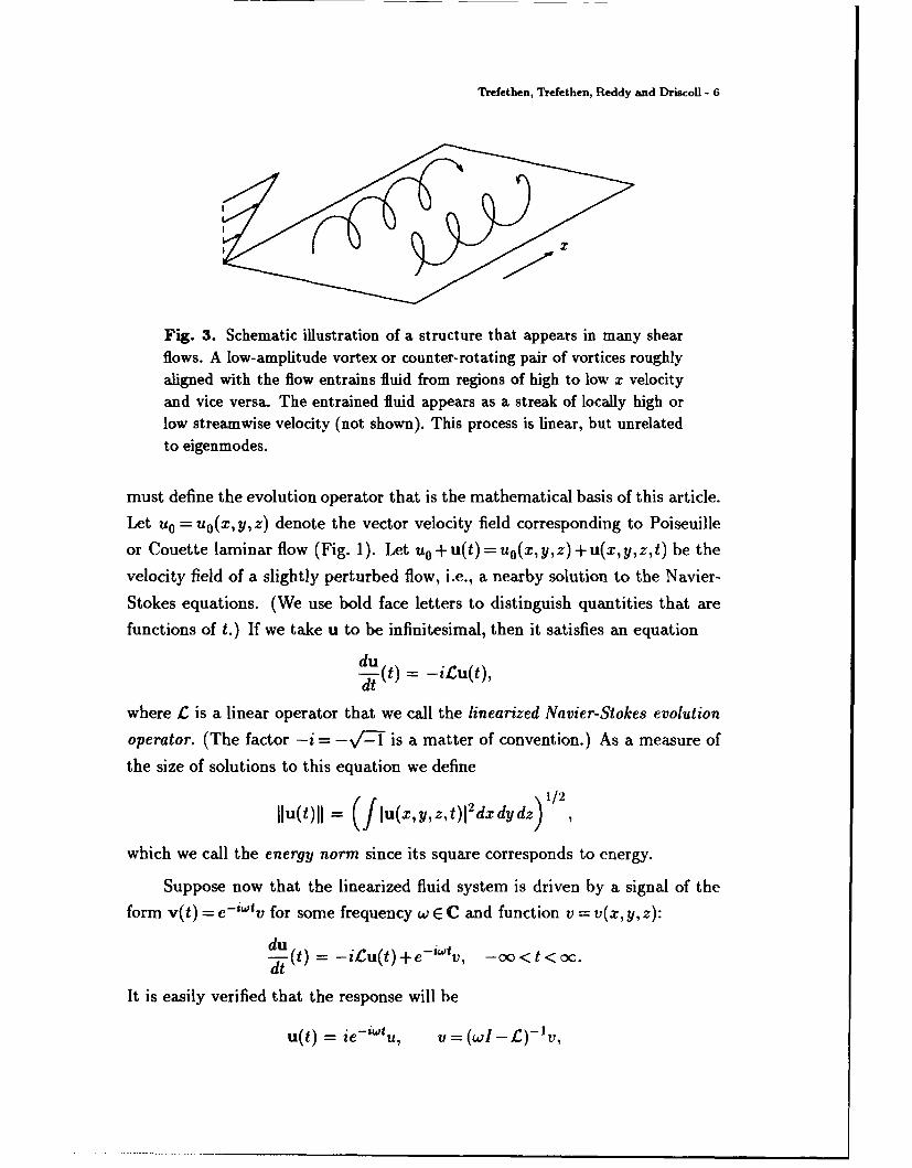
Fig. 3. Schematic illustration of a structure that appears in many shearflows. A low-amplitude vortex or counter-rotating pair of vortices roughlyaligned with the flow entrains fluid from regions of high to low x velocityand vice versa. The entrained fluid appears as a streak of locally high orlow streamwise velocity (not shown). This process is linear, but unrelatedto eigenmodes.

must define the evolution operator that is the mathematical basis of this article.

Let u0 = uo(X, y, z) denote the vector velocity field corresponding to Poiseuille

or Couette laminar flow (Fig. 1). Let u 0 + u(t) = uo(x, y, z) + u(x, y, z, t) be the

velocity field of a slightly perturbed flow, i.e., a nearby solution to the Navier-

Stokes equations. (We use bold face letters to distinguish quantities that arefunctions of t.) If we take u to be infinitesimal, then it satisfies an equation

du-Tt Mt = 1Ct)

where C is a linear operator that we call the linearized Navier-Stokes evolution

operator. (The factor -i = -j- is a matter of convention.) As a measure of

the size of solutions to this equation we define

11u(t)0 = (J'u(x,y,z,t)12dxdydz)1/2,

which we call the energy norm since its square corresponds to energy.

Suppose now that the linearized fluid system is driven by a signal of the

form v(t) = e-iwtv for some frequency w E C and function v = v(x, y, z):

du = -i'u(t) + e-iJ tv, -00 < t < OC.

It is easily verified that the response will be

u(t) = ie-&"u, u = (wI-C£)-'v,


where I denotes the identity operator. Thus the operator (wII-C)-', known as

the resolvent of C, transforms "inputs" v to the linearized fluid flow at frequency

w into corresponding "outputs" u (10, 11). The degree of amplification that may

occur in the process is equal to the operator norm

def suIuhI(wI-LY 1It - sup

,,AO Ilvll"

Since an arbitrary time-dependent perturbation of the laminar flow can be re-

duced to an integral over real frequencies by Fourier analysis, values of W on the

real axis are of particular interest. The maximum possible amplification over

all real frequencies is supWER I1(wI-C)-1 11, and this is the quantity plotted in

Fig. 2.

An eigenvalue of £ is a number w E C such that Lu = wu for some corre-

sponding eigenfunction u. Equivalently, it is a number w with the property that

inputs with frequency w can be amplified unboundedly: II(wI -,C)-11 = 0.

More generally, for any c > 0, an f -pseudo-eigen value of C is a number W

such that jj(wI- £)-1 _ -, and a corresponding f-pseudo-eigenfunction or

c-pseudomode is any function u with 1IICu-wull _< clull. If c is very small, then

an c-pseudomode u may be excited to a substantial axaplitude by a very small

input, possibly including noise in an experimental apparatus. At R = 5000, for

example, a streamwise streak is an c-pseudomode of the linearized Poiseuille

flow problem for e t 1.2 x 10-5 (Fig. 2) and thus can be excited by a streamwise

vortex five orders of magnitude weaker in amplitude.

The set of E-pseudo-eigenvalues of an operator is the c-pseudospectrum (27):

AJ(C) = {wEC: II(wI-C)-'lIC"1}.

The pseudospectra {AJ(C)} form a nested family of sets in the complex plane,

with A0 (£C) equal to the spectrum A(£). If £ is normal, AJ(C) is the set of

all points at distance <,E from A(£), but in the non-normal case it may be

much larger. The physical significance of pseudospectra can be described as

follows. If a system is governed by a linear operator that is normal or close to

normal-familiar examples include musical instruments, oscillating structures,

and molecules as described by quantum mechanics--then the frequencies at

which it resonates strongly are determined by its spectrum. The resonances of

a system that is far from normal, however, can only be understood by examining

its pseudospectra.


Spectra and pseudospectra

Figs. 4 and 5, the centerpieces of this article, depict spectra and pseu-

dospectra for Couette flow at R = 350, 3500 and Poiseuille flow at R = 1000,

10000. These Reynolds numbers roughly span the range in each case from pos-

sible turbulence (in some experiments) to unavoidable turbulence (even in ex-

periments under the most carefully controlled conditions). These and our other

figures are the results of numerical computations. As a practical matter we first

Fourier transform in x and z, reducing the calculation to one space dimension

(y) and two real parameters a, 3 (wavenumbers in x, z). The generation of each

figure then requires a minimization in the a-03 plane (28).

Spectra of £Cf for particular values of a and 13 have been published by var-

ious authors (5, 29), and pseudospectra of Cc# will appear in (12, 16). Neither

spectra nor pseudospectra of £ itself have been plotted previously.

Fig. 4 reveals that in the case of Couette flow, the spectrum of £ is a contin-

uous region contained in the lower half-plane. (For each a, 13 pair the spectrum

is discrete, but the union over a and )3 is a continuum, shown in the figure as

a shaded region.) This is true for all R, corresponding to the unconditional

stability of Couette flow according to eigenvalue analysis. The spectrum comes

closest to the upper half-plane along the imaginary axis, at a distance O(R-1)

as R -+ oc. The pseudospectra of £, by contrast, protrude significantly into the

upper half-plane, indicating that evolution process governed by this operator

will feature prominent non-modal effects.

One cannot see in Fig. 4 what values of a and 13 correspond to various

points in the spectrum and pseudospectra. The situation is roughly as follows.

The upper boundary of the spectrum corresponds to 1 = 0 and to values of a

that grow in proportion to Rew. In the pseudospectra, the values of a are

comparable but the values of 13 are 0(1). This difference in values of 3 reflects

the fact that although the dominant eigenmodes of this problem are 2D, the

dominant pseudomodes are 3D.

Fig. 5 reveals the more complicated situation for Poiseuille flow. The pseu-

dospectra are qualitatively similar, again extending well into the upper half-

plane (30). The boundary of the spectrum, however, is now determined by two


0.1( Couette, R=350

Im(w)

Re (w)-1 0

0.1 (B) Couette, R=3500

Im(R)

-1 0

Fig. 4. Spectrum and E-pseudospectra in the complex w-plane of the lin-

earized Navier-Stokes evolution operator for Couette flow at R = 350 and

3500. The spectrum is the shaded region, and the solid curves, from outer to

inner, are the boundaries of the e-pseudospectra with c = 10-2, 10-215,10-3,

10-3.5. The spectrum lies in the lower half-plane, but the pseudospectra ex-

tend significantly into the upper half-plane, revealing the non-normality of

this operator. Note that the real and imaginary axes are scaled differently.


0. 1 (A) Poiseujile, R = 1000

___________ - - ~Re(La)-1 ~01

0.1- (B) Poise~uille,R=00

Re (w)01

Fig. 5. Same as Fig. 4 but for Poiseuille flow with R =1000, 10000. ForR > 5772, two bumps in the spectrum extend into the upper half-plane.However, the large lobes of the pseudospectra along the imaginary axis arephysically more important.

Trefethen, Trefet hen, Reddy and Driscoll - 11

distinct components, each with # = 0. One of these looks qualitatively like the

boundary of the spectrum for Couette flow and corresponds to perturbations

of the flow field that are symmetric about the centerline. The other is very

different, consisting of bumps on either side of the origin corresponding to an-

tisymmetric perturbations of the flow. For lower values of R, the spectrum is

contained in the lower half-plane, but at R = 5772 the bumps cross the real

axis. These bumps represent the mode that has received most of the attention

in the literature, which is sometimes known as a Tollmien-Schlichting or TS

wave. However, their negligible effect on the nearby pseudospectral contours

reveals that this mode is oriented at a sizable angle to the remainder of the

system (31). The pseudomodes associated with wL 0-streamwise streaks with

a : 0, /3 # 0--are physically more important.

We can summarize the implications of Figs. 4 and 5 by noting that whereas

spectral analysis suggests that plane Couette and Poiseuille flows are fundamen-

tally different, since one has unstable eigenmodes for certain values of R and the

other does not, pseudospectral analysis suggests that they are fundamentally

similar, as is observed in experiments.

Resonance curves

Figs. 6 and 7 represent slices of Figs. 4 and 5 along the real axis. In

each figure II(wI - C)-'l is plotted as a function of w E R for several values

of R, indicating the factors by which linearized Couette and Poiseuille flows are

capable of amplifying time-dependent perturbations at various real frequencies.

When the amplification is large we speak of the phenomenon of resonance,

although a more careful term might be "pseudo-resonance."

For Couette flow, no significant resonance is present except near w = 0.

There, the amplification may be powerful indeed, reaching a value 0(R 2) al-

though the spectrum lies at a distance O(R- 1) below the real axis. For Poiseuille

flow, the behavior for w • 0 is similar, but for R > 5772 an additional resonance

for larger w appears due to the unstable eigenmode. In principle, this mode

would dominate if one could set up an experiment involving a sufficiently long

channel and a sufficiently smooth flow. Under conditions where this can happen,

however, low-frequency inputs are already subject to non-modal amplification

by a factor of order 105.


106

105

{I(w!-C•)-'f{

104,

S~R = 3500

103

SR = 1000

R =_ 350102-•

-0.1 0 0.1 0.2 0.3 0.4

Fig. 6. Resonance or "pseudo-resonance" curves for Couette flow. Eachcurve shows 11(wI-C)-l1I, the maximum possible amplification of pertur-

bations to the laminar flow field at frequency w.

106

105 R =10000

104\"f(wJI- C)-1 'JJ •..

R=3000

103 R/=100

R =300

102

10113

-0. 1 0 0.1 0.2 0.3 0.4

Fig. 7. Like Fig. 6 but for Poiseuille flow. For R > 5772 infinite amplifica-tion is possible in principle, but of doubtful significance in practice.


Transient energy growth

Another aspect of linear, non-modal instability of fluid flows is the transient

amplitude or energy growth that may evolve from certain initial conditions. This

is the phenomenon that has been studied in the recent papers by Gustavsson,

Butler and Farrell, and Reddy and Henningson, where many more physical

details can be found.

Mathematically, consider the initial-value problem

du (t) = -iZCu(t), t > 0, u(0) = v.

The solution can be written u(t) = exp(-it1)v, where exp(-itI) is the operator

exponential. The factor by which such solutions can grow in time t is

11exp(-it12)II = sup Ilu(t)_ _

and the energy growth is the square of this quantity. If C were a normal operator

with spectrum in the lower half-plane, we would have Ilexp(-iLtC)I < 1 for all

t > 0. In actuality, Gustavsson and Butler and Farrell discovered that the growth

is Ilexp(-itC)I1 = O(R), making the energy growth O(R 2 ).

Fig. 8 illustrates this phenomenon for Couette flow at various Reynolds

numbers. The agreement of the curves for finite R and R = oo can be explained

as follows: the streamwise vortex/streak mechanism of energy growth is inviscid,

and operates on a time scale O(R) before being shut off by the effects of viscosity.

Such behavior is physically straightforward, appearing complicated only when

interpreted in the basis of eigenmodes.

Fig. 9 gives further information for Couette flow with R = 350; other

Reynolds numbers are qualitatively similar. The restriction to x-independent

flows (a = 0) curtails the transient growth somewhat for small t but has no ef-

fect for larger t, when the maximal growth is achieved with a = 0 anyway (i.e.,

a purely streamwise structure). The restriction to z-independent flows (0 = 0),

however, has a huge effect, shutting off most of the transient growth except fort (32).

The O(R 2 ) resonances of Figs. 2,6,7 are approximately equal to the inte-

grals under the curves in Figs. 8 and 9. Mathematically, this can be seen from

Trefethen, Trefethen, Reddy and Driscon - 14

1.50 22500

R = 4000

R = 0 3500

3000100- 1/------ 0000

Amplitude 250Energy11 exp( -it£C)[[ 200 11 exp( -itC I)[

t0 100 200 300 400 500

Fig. 8. Non-modal transient energy growth for Couette flow. For anyfinite R, the effect of viscosity shuts off the growth on a time scale O(R).

12 144

Amplitude 0=0 Energy

Ilexp(-it C)j lexp(-iti )12

8 lower bound 64based onpseudospectra

4- 16

,30 (2D)

0 t0 20 40 60 80 100 120 140

Fig. 9. Transient growth for Couette flow at R = 350. Little growth occurswhen only 2D perturbations are allowed.


100 1000 5000 10,000 25,000 50,000

ki

k' 75,000

00

0 1 __ I --------------.... ... R

0 5M00 10000 15000 2M000

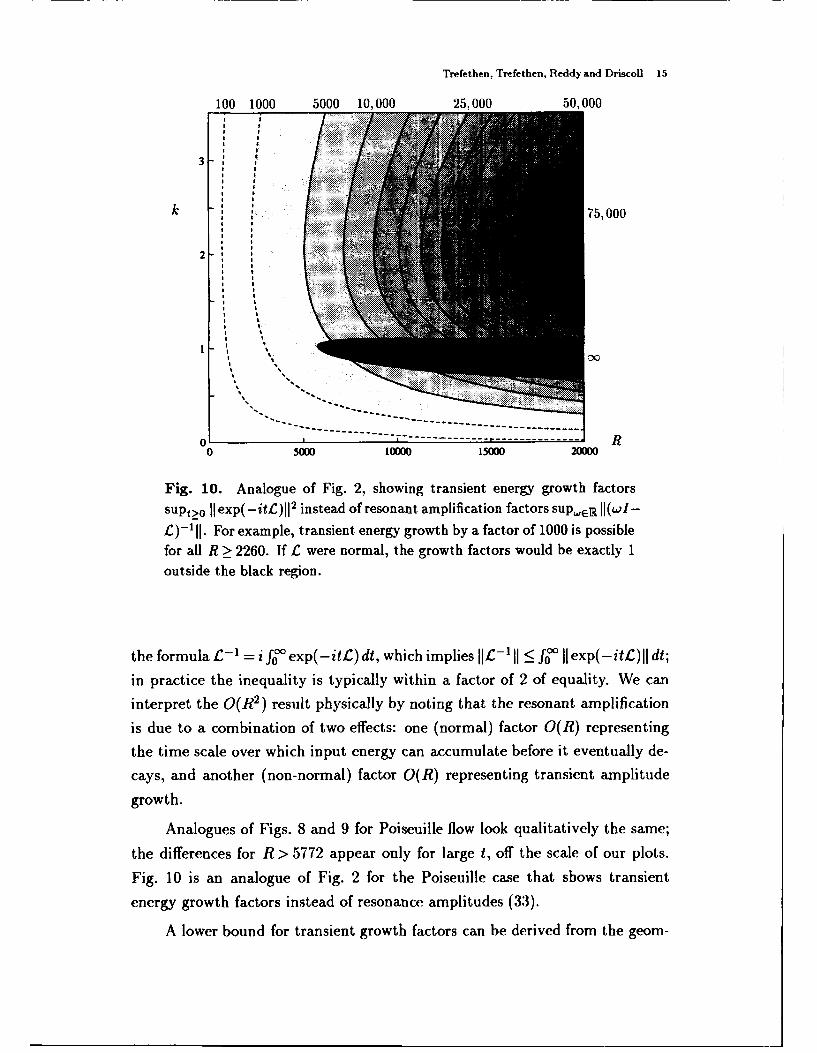
Fig. 10. Analogue of Fig. 2, showing transient energy growth factors

supt>0 I exp(-itC)112 instead of resonant amplification factors sup,,WR 11(WI-

C)-1 II. For example, transient energy growth by a factor of 1000 is possiblefor all R > 2260. If C were normal, the growth factors would be exactly 1

outside the black region.

the formula £-1 =i f~o exp(-itL) dt, which implies IILt-' II f II exp(-itC)II dt;

in practice the inequality is typically within a factor of 2 of equality. We can

interpret the O(R 2 ) result physically by noting that the resonant amplification

is due to a combination of two effects: one (normal) factor O(R) representing

the time scale over which input energy can accumulate before it eventually de-

cays, and another (non-normal) factor O(R) representing transient amplitude

growth.

Analogues of Figs. 8 and 9 for Poiseuille flow look qualitatively the same;

the differences for R > 5772 appear only for large t, off the scale of our plots.

Fig. 10 is an analogue of Fig. 2 for the Poiseuille case that shows transient

energy growth factors instead of resonance amplitudes (33).

A lower bound for transient growth factors can be derived from the geom-


etry of the pseudospectra in the complex upper half-plane. One can show:

supllexp(-it£)jj >! sup c-lor'(£),f>0 C>0

where ao(12) = sup-EA,((,)Imw is the c-pseudospectral ordinate of C (11, 16).

In words, if the pseudospectra protrude far into the upper half-plane, then sub-

stantial transient energy growth must be possible. The horizontal line segment

in Fig. 9 marks this lower bound, which falls short of the true maximum by

only about a factor of 1.4 in amplitude or 2.0 in energy, numbers typical of both

Couette and Poiseuille flows for a wide range of R (3, 34).

Physically interesting pseudomodes

Instead of operator norms, it is customary in the literature to investigate

the evolution of particular solutions chosen for one physical reason or another.

The amplitude history of the solution with initial flow field u(O) = v is given by

1I exp(-it£)vII, and the upper envelope of all such curves, corresponding to all

initial functions v, is the operator norm 1I exp(-it£)[1 that we have discussed.

Three choices of v with particular claims to attention can be identifiedwith the aid of the singular value decomposition (SVD), the natural tool for all

kinds of questions involving norms and extrema of nonsymmetric matrices and

operators (35). Fig. 11 displays the curves 11 exp(-it£)vjI corresponding to the

principal right singular vectors of the following operators:

vl: exp(-i0+12) (maximal initial growth rate),

v2 : exp(-itopt£) (maximal total growth),

V3 : £-1 (maximal resonance).

The function v1 is the perturbation with maximal growth rate at t = 0, a function

that has been studied by Serrin, Busse, Joseph, Lumley, and others (2, 8, 15,

36). (The notation exp(-i0O+,) indicates the limit of the SVD of exp(-it£)

as t -4 0. A cleaner and computationally more appropriate characterization of

the function v, is that it is the principal eigenfunction of (1 - L*)/2i, with

growth rate at t = 0 equal to the corresponding eigenvalue, or equivalently, to

the distance that the numerical range of C protrudes into the upper half-plane.)

The function v2 is the Butler-Farrell "optimal" that achieves maximal total


144

Amplitude -. ! 3 : maximal resonance EnergyI]exp(-it£)vjj [11exp(-it £)vjj'

81 64

i /// V2." Butler-Farrell//•..• • optimal"

4- • v,: maximal initial 16

0' t0 40 80 120

Fig. 11. Initial growth and eventual decay resulting from three particularinitial perturbations v for Couette flow at R = 350. The dashed curve isthe operator norm of Fig. 9.

growth at some time t = topt. The function v3 is the one that excites a maximal

resonant response in the sense of Figs. 2,6,7.

Fig. 11 reveals that although the physical ideas behind the functions vj,

v2, v3 are different, v2 and v3 at least lead to comparable energy growth. These

functions are also similar in structure: both have approximately the form of

streamwise vortices that evolve into streamwise streaks (corresponding to left

rather than right singular vectors of the same operators). An analogous figure

for Poiseuille flow looks roughly similar, but the gap between v2 and v3 is smaller

and the gap between these and v1 is larger.

Trefethen, Trefet hen, Reddy and Driscoll 18

The inviscid limit

The relationship between the stability theories for viscous and inviscid flows

has been an awkward one (21). It is natural to expect that the mechanism of

instability should be essentially inviscid, so that it should be possible to get at

the essence of the matter by setting R= oc, simplifying the equations greatly.

Yet the results of inviscid stability analysis have generally matched neither the

results of viscous analysis nor experimental observations. A conspicuous exam-

ple is Rayleigh's theorem of 1880 (37), which asserts that unless the velocity

profile contains an inflection point, an inviscid parallel shear flow is always sta-

ble, a conclusion plainly at odds with the observed behavior of Poiseuille and

Couette flows at large finite Reynolds numbers.

We believe that much of the difficulty with the limit R -- oc has been due

to misunderstanding of the significance of eigenvalues. Rayleigh's theorem, like

Squire's theorem, is actually a statement about the existence of eigenvalues in

the upper half-plane, and like Squire's theorem, it is mathematically correct but

misleading. If one defines stability by energy growth instead of by eigenvalues,

one finds that every planar shear flow with R = oo is unstable, regardless of the

velocity profile. This observation is due to Ellingsen and Palm (38), with roots

going back to Kelvin, and related results have been established by many others

(23, 39). The example of Couette flow with R = oc and a = 0 is particularly

simple, for the equations reduce to the 2 x 2 block matrix problem

where i and ý represent the y components of velocity and vorticity (functions

of y, after Fourier transformation in x and z). The matrix L in this equation

is defective (i.e., nondiagonalizable), with 11exp(-itL)Q1 -, Ct as t --+ c for some

constant C = C(,6) < 1 (after transformation to the energy norm). Thus inviscid

Couette flow is linearly unstable, even though there is no exponentially growing

eigenmode, which explains the dashed line in Fig. 8.

This "algebraic" instability of inviscid flows is well known among hydro-

dynamicists. What has been missing is a fully satisfactory link to the case of

viscous flows, where the evolution operator is typically nondefective and eigen-

value analysis has been accepted as a test of stability. The point that has not.

Trefethen, Trefethen, Reddy and Driscoll 19

always been appreciated is that although a flow may be stable in the sense of

bounded response to infinitesimal perturbations for each finite R, it does not

follow that it satisfies any bound uniformly as R -* oc. In the absence of a

uniform bound, the notion of stability for large finite Reynolds numbers has

little meaning (40).

Our computations indicate that by most measures, the limit R --+ 0 is a

smooth one. Table 1 summarizes the behavior of a number of quantities in this

limit and may serve as a reference point for most of our figures (41).

Couette Ca 3 Poiseuille a /

distance of spectrum from real axis (R/2.47)- 1 0 0 (R/2.47)- 1 0 0

max. resonance supIElJ(wI-L)-IIl (R/8.12) 2 0 1.18 (R/17.4) 2 0 1.62

transient growth sup,>o11exp(-itL)11 2 (R/29.1) 2 35.7/R 1.60 (R/71.5) 2 0 2.04

optimal time topt R/8.52 " " R/13.2

lower bound based on pseudospectra (R/42.6)2 0 1.62 (R/103.) 2 0 2.04

transient growth (a = 0) (R/29.3) 2 0 1.66 (R/71.5)2 0 2.04

Table 1. Leading-order behavior of various quantities as R - oc. These

formulas are accurate to at least 1% for all R > 100. The results forPoiseuille flow pertain to the highly non-normal part of the problem, ig-noring the R > 5772 mode (TS wave).

Destabilizing perturbations and secondary instability

There is an alternative, equivalent definition of the pseudospectra of an

operator £ (27, 42):

AJ(C) = closure{wE C: wE A(C +E) for some E with 1C11 <

In words, the c-pseudospectrum of £ is the union of the spectra of all perturbed

operators £+E with IIII •1 c, together with any limit points of this set (a tech-

nicality of little importance). It is interesting to reconsider the implications

of Figs. 4 and 5 in the light of this alternative characterization. The pseu-

dospectral boundary contours in these figures imply that. although the flows in

question are eigenvalue stable (for R < 5772 in the Poiseuille case), exceedingly

Trefethen, Trefethen, Reddy and Driscoll 20

"10-

10-7

104 Poiseujille

10" L

11-7

10.

102 10R

Fig. 12. An eigenvalue stable shear flow at Reynolds number R can bedestabilized by a linear operator perturbation £ of norm "min = O(R-2);the dependence is so nearly quadratic that the curves appear straight toplotting accuracy. The inverse E-I = O(R 2) is equal to the maximal res-onant amplification plotted in Fig. 2. The circles mark the approximate

Reynolds numbers (350, 1000) at which Couette and Poiseuille flows areobserved to undergo transition to turbulence.

small perturbations to the evolution operator, of order O(R 2 ), suffice to make

them eigenvalue unstable. The norm of the minimal destabilizing perturba-

tion is rmin = (supwER j[(wI--C)--1j)-I, i.e., the inverse of the quantity plotted

in Fig. 2 and labeled maximal resonance in Table 1. This observation pro-

vides a new interpretation of Fig. 2. For example, although Poiseuille flow with

R = 5000 is eigenvalue stable, there exists a perturbation E of norm 1.21 x 10-5

that renders it unstable. See Fig. 12.

This raises the question of the physical meaning of operator perturbations

and what relevance they may have to flow instabilities observed in the labora-

tory. (We emphasize that g is a perturbation of £, not of the flow field u0 .)

The minimal destabilizing perturbation E with 11,F1 = cmin is easily character-

ized: it is a rank-i operator of the form uvui*, where or, v, u are the principal

singular value and right and left singular vectors of C-1, respectively. This op-

erator transforms streamwise streaks into streamwise vortices, thereby closing

frefethen, Trefet hen, Reddy and Driscoll - 21

the loop so that the transient growth of Figs. 8-9 can feed back upon itself tobecome modal growth for all t. Of course there is no reason to expect such

a perfectly contrived perturbation to arise under natural conditions. What is

suggestive is that even random perturbations of C have qualitatively the sameeffect. At R = 5000, for example, approximately 90% of all random perturba-

tions E to C with JIS1 = 10-3 render a Poiseuille flow eigenvalue unstable, where

by a random perturbation we mean an elementwise random perturbation of the

20 x 20 matrix that represents the projection of £ onto the space spanned by its

20 dominant eigenmodes (with fixed a = 0 and ,3 = 1.62). Though it is a large

step from such matrices to shear flows, the possibility is clearly suggested that

seemingly negligible perturbations may destabilize a flow even in the narrow

eigenvalue sense. One can imagine that imperfections in the boundary walls of

a laboratory apparatus, for example, might have this effect. We hope that fu-

ture investigations will reveal whether this idea of perturbed evolution operators

provides an explanation of instability in some flows.

A different prospective application of the idea of destabilizing operator per-

turbations may be to the theory of "secondary instability" as an explanation ofsubcritical transition to turbulence (8, 9). This theory is founded on the discov-

ery that when certain laminar shear flows are perturbed by certain physically

motivated waves of large amplitude, the resulting problem is eigenvalue unsta-

ble, with eigenvalues high enough in the upper half-plane to match observed

time scales for transition. The great sensitivity of the spectrum of C to pertur-

bations, however, raises the question of whether similar eigenvalue instabilities

might also arise with the use of more or less arbitrary perturbations, not justthe ones that hzve been considered based on physical arguments.


Nonlinear bootstrapping and transition to turbulence

Kelvin wrote in 1887 (19):

It seems probable, almost certain indeed, that... the steady motion is stable forany viscosity, however small; and that the practical unsteadiness pointed out byStokes forty-four years ago, and so admirably investigated experimentally fiveor six years ago by Osborne Reynolds, is to be explained by limits of stabilitybecoming narrower and narrower the smaller is the viscosity.

This view of instability is still the standard one, but to this day, it has never been

confirmed in detail. In this final section we would like to speculate about what

the eventual confirmation may look like-in other words, about how nonlinear

and linear mechanisms interact to bring about transition to turbulence.

Consider the 2 x 2 nonlinear model problem

du = Au + IlullBu, A -RI 1)dt 0\O -2R-'1

where R is a large parameter. The linear term, involving the non-normal ma-

trix A, amplifies energy transiently. The nonlinear term, involving the skew-

symmetric matrix B, rotates energy in the U1 -U2 plane but does not directly

create or destroy energy, since it acts orthogonally to the motion (43). Thus

we have linear amplification coupled with energy-neutral nonlinear mixing, a

situation that holds also for the equations of fluid mechanics (44).

Fig. 13 shows norms I1u(t)[I for solutions starting from eight different initial

vectors of the form u(p) = (Oconst)T, with R = 25. For Ilu(0)]1 < 10-4, the

curves are approximately translates of one another on this log scale, indicating

that the evolution is effectively linear. At I1u(0)II = 4 x 10-4, the nonlinearity

has begun to have a pronounced effect. At 11u(0)]I = 5 x 10-4 the threshold has

been crossed, and for this and higher amplitudes, the curves do not decay to

zero but blow up to a critical point of amplitude ; 1.

Fig. 13 reveals a remarkable phenomenon: the amplitude growth is far

greater than that of the purely linear problem du/dt = Au. Table 2 lists the

linear growth factor M - R/4 and the threshold amplitude f (for this particular

choice of initial vector) for four values of R. Evidently c is of order M-', not

M- 1. This "bootstrapping" effect can be explained as follows. Suppose the

solution at t = 0 consists of a vector of amplitude ( in a direction that excites


1001,,j(0)11 10-2 I1,,(0)1 = 10 -' I1,,(0)11 = 5 x 10-4100;Ilu(t)It LINEAR/NONLINEAR

"BOOTSTRAPPING"

10-2J1-u(0)II = 4 x 10- 1 PURELY

LINEARGROWTH

10-6 _

7 t

0 100 200

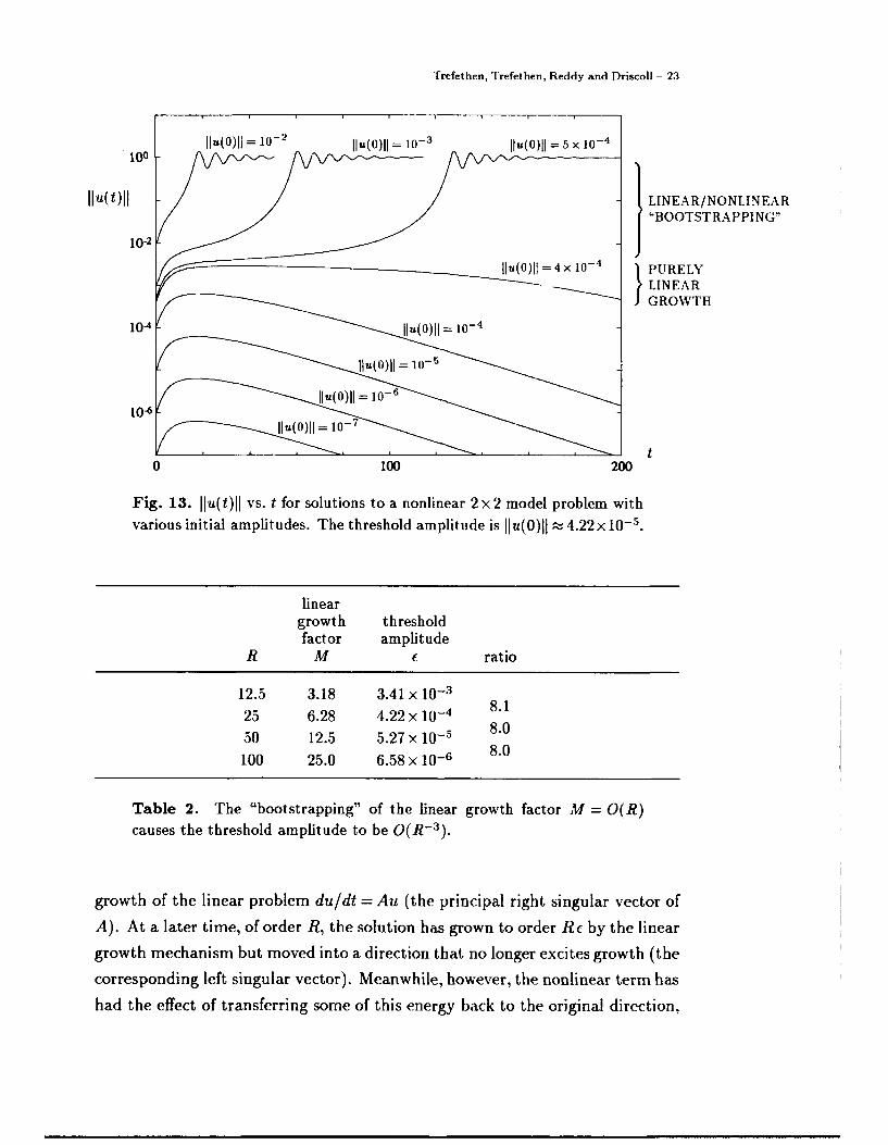
Fig. 13. Ilu(t)Il vs. t for solutions to a nonlinear 2 x 2 model problem withvarious initial amplitudes. The threshold amplitude is Ilu(0)Il 4.22x 10-5.

lineargrowth thresholdfactor amplitude

R M C ratio

12.5 3.18 3.41 x 10-325 4 8.1

25 6.28 4.22 x 10- 8

50 12.5 5.27 x 10-5 8.0

100 25.0 6.58 x 10-6 8.0

Table 2. The "bootstrapping" of the linear growth factor M = O(R)causes the threshold amplitude to be O(R- 3 ).

growth of the linear problem du/dt = Au (the principal right singular vector of

A). At a later time, of order R, the solution has grown to order RC by the linear

growth mechanism but moved into a direction that no longer excites growth (the

corresponding left singular vector). Meanwhile, however, the nonlinear term has

had the effect of transferring some of this energy back to the original direction,

Trefethen, Trefet hen, Reddy and Driscoll 21

with amplitude R(RC) 2 = R 3 C2 since the nonlinearity is quadratic and the time

scale is O(R). If R 3C2 is of order less than -, the process is not. self-sustaining

and the energy dies away. On the other hand if R3 '- is of order greater than .,

then there is more energy than was present at the start and feedback occurs,

leading to self-sustained amplitude growth. Thus the threshold amplitude is

O(R- 3 ).

A similar experiment shows that if the same nonlinear equation is driven

by a forcing oscillation eOwtv instead of an initial vector u(O), the threshold

amplitude becomes E = O(R- 4 ).

It may appear at first sight that these results indicate the great power and

importance of nonlinear effects. Yet in two senses, these energy growth scenar-ios are essentially linear. First, as mentioned above, the nonlinear term does

not add energy locally but merely redistributes it. Second, the appearance of

the bootstrapping phenomenon does not depend on the precise nature of the

nonlinearity. Any quadratic nonlinear term that transfers energy from decayingto growing solution components has the potential of inducing a threshold ampli-

tude c = O(R- 3 ) or O(R-4 ) with respect to initial or forcing data, respectively;

a random perturbation, for example, will often suffice. Higher-order nonlinear-ities also lead to similar effects, though the exponents may be lowered, e.g. to

S= O (R -2 ) and O (R - 3 ) for a cubic nonlinearity.

The Navier-Stokes equations are certainly more complicated than our 2 x 2

model. One difference is that instead of 2-vectors, they act on functions with

infinitely many degrees of freedom, most of which do not experience non-normal

linear growth. There will always be some energy in the growing pseudomodes,

however, and in a pipe or channel of substantial extent., random fluctuations

can be expected to raise the energy levels in such components locally well about,

the statistical average (45, 46). Another difference is that the nonlinear in-

teractions in the Navier-Stokes equations act across different wave numbers o

and 0 (13, 14), making the exponent of 2 in our model perhaps unrealistically

low. Despite these qualifications, we conjecture that the transition to turbu-

lence of eigenvalue-stable shear flows proceeds analogously to our model in that.

the destabilizing mechanism is essentially linear in the senses described above,with an amplitude threshold for transition of order O(R' ) for some a < -1.

Trefethen, Trefet hen, Reddy and Driscoll - 25

Conclusion

In this article we have described three essentially linear approaches to the

phenomenon of instability of shear flows: (i) (pseudo-) resonance, (ii) transient

energy growth, and (iii) destabilizing operator perturbations. These ideas are by

no means independent. Mathematically, they are all related to the pseudospec-

tra of the operator L, and physically, they all depend on the same mechanisms

of extraction of energy from the mean flow by streamwise vortices and other

structures. One should not expect that any one of these ideas will necessarily

prove to be the "right" one, but rather, that each of them may prove appropriate

to a particular class of experiments. For example, it is reasonable to speculate

that in different situations transition to tui uiuence may be primarily triggered

in physically quite different ways by (i) laboratory vibrations, (ii) initial or in-

let disturbances, or (iii) deviations of the pipe or channel geometry from the

Poiseuille or Couettc ideal.

It is likely that in the upcoming decade, great progress will be made in elu-

cidating these details. Numerical simulations of the 3D Navier-Stokes equations

are becoming routine, and in the next few years such simulations will probably

settle at last the question mentioned in the last section, for example, of how the

threshold amplitude for transition depends on the Reynolds number in various

flow situations.

Besides hydrodynamic stability, there are other fields also where highly

non-orthogonal eigenfunctions arise and eigenvalues may be misleading. Exam-

ples in fluid mechanics include the instability of magnetic plasmas (48) and the

formation of cyclones (49). Two more examples come from the field of numeri-

cal analysis: the numerical instability of discretizations of differential equations

(40) and the convergence of iterative algorithms for nonsymmetric systems of

linear equations (50). The recurring theme in these and other applications is

that although the long-time behavior of an evolving system may be controlled

by nonlinearities, some important phenomena are of a short-time nature and

essentially linear (51, 52). If the linearized problem is far from normal, eigenval-

ues may be precisely the wrong tool for analyzing it, for eigenva!ues determine

the long-time behavior of a non-normal linear process, not the transient. We

can expect to see further examples of alternatives to eigenvalues in the years

ahead.

Trefcthen, Trefethen, Reddy and Driscoll - 26

REFERENCES AND NOTES

1. P. G. Drazin and W. H. Reid, Hydrodynamic Stability (Cambridge U. Press, 1981).

2. D. D. Joseph, Stability of Fluid Motions I (Springer Verlag, 1975).

3. This article is adapted from L. N. Trefethen, A. E. Trefethen, S. C. Reddy, Technical ReportNo. TR 92-1291 (Department of Computer Science, Cornell University, 1992). Readersinterested in additional details are urged to contact the first author for a copy of thisreport.

4. The Reynolds number is defined by R = L Vp/p, where L is the half-width of the channel,V is the maximum velocity, p is the density, and p is the viscosity. The distance, velocity,and time variables in our equations are nondimensionalized by L, V, and L/V, respectively.

5. S. A. Orszag, J. Fluid Mech. 50, 689 (1971).

6. S. J. Davies and C. M. White, Proc. Roy. Soc. A 119, 92 (1928); V. Patel and M. R. Head,J. Fluid Mech. 38, 181 (1969); D. R. Carlson, S. E. Widnall, and M. F. Peeters, ibid. 121,487 (1982).

7. N. Tillmark and P. H. Alfredsson, J. Fluid Mech. 235, 89 (1992).

8. S. A. Orszag and A. T. Patera, J. Fluid Mech. 128, 347 (1983).

9. B. J. Bayly, S. A. Orszag, T. Herbert, Ann. Rev. Fluid Mech. 20, 359 (1988).

10. T. Kato, Perturbation Theory for Linear Operators (Springer-Verlag, 1976).

11. A. Pazy, Semigroups of Linear Operators and Applications to Partial Differential Equations(Springer-Verlag, 1983).

12. S. C. Reddy, P. J. Schmid, D. S. Henningson, SIAM J. Appl. Math. 53, in press.

13. L. H. Gustavsson, J. Fluid Mech. 224, 241 (1991).

14. D. S. Henningson, in Advances in Turbulence, A. V. Johansson and P. H. Alfredsson Eds.(Springer-Verlag, 1991), pp. 279-284; D. S. Henningson, A. Lundbladh, A. V. Johansson,J. Fluid Mech., in press.

15. K. M. Butler and B. F. Farrell, Phys. Fluids A 4, 1637 (1992).

16. S. C. Reddy and D. S. Henningson, "Energy growth in viscous channel flows," to appear.

17. Closely related recent developments are described in K. S. Breuer and J. H. Haritonidis,J. Fluid Mech. 220, 569 (1990) and Y. Bun and W. 0. Criminale, "Evolution of threedimensional disturbances in a mixing layer," submitted.

18. See, e.g., Figs. 4.11, 4.15, 5.5 of (1). To be precise, the figures that have appeared in theliterature have the x wavenumber a as the ordinate, not the x-z wave number magnitudek= (a2+,62)112, and thus correspond to 2D perturbations only. This changes the upperboundary in such a way that the black region shrinks to zero width as R--oo.

19. Lord Kelvin (W. Thomson), Phil. Mag. 24,188 (1887).

20. W. M'F. Orr, Proc. Roy. Irish Acad. A 27, 9 and 69 (1907).

21. K. M. Case, J. Fluid Mech. 10, 420 (1960) and Phys. Fluids 3, 143 (1960).

https://www.researchgate.net/publication/231787467_Energy_in_Viscous_Channel_Flows?el=1_x_8&enrichId=rgreq-a87e10a04a3eb27ca57dead8e6ff6ddd-XXX&enrichSource=Y292ZXJQYWdlOzI0MzIyNTg2O0FTOjEwMTY3NjUxNDAyMTM3OEAxNDAxMjUyOTc4MTQ1

https://www.researchgate.net/publication/234351179_Stability_of_Fluid_Motions_I?el=1_x_8&enrichId=rgreq-a87e10a04a3eb27ca57dead8e6ff6ddd-XXX&enrichSource=Y292ZXJQYWdlOzI0MzIyNTg2O0FTOjEwMTY3NjUxNDAyMTM3OEAxNDAxMjUyOTc4MTQ1

https://www.researchgate.net/publication/230801964_Perturbation_Theory_of_Linear_Operators?el=1_x_8&enrichId=rgreq-a87e10a04a3eb27ca57dead8e6ff6ddd-XXX&enrichSource=Y292ZXJQYWdlOzI0MzIyNTg2O0FTOjEwMTY3NjUxNDAyMTM3OEAxNDAxMjUyOTc4MTQ1

Trefethen. Trefethen, Reddy and Driscoll - 27

22. G. Rosen, Phys. Fluids 14, 2767 (1971); D. J. Benney and L. H. Gustavsson, Stud. App).Math. 64, 185 (1981); L. S. Hultgren and L. H. Gustavsson, Phys. Fluids 24, 1000 (1981),B. F. Farrell, ibid. 31, 2093 (1988).

23. A. D. D. Craik and W. 0. Criminale, Proc. Roy. Soc. A 406, 13 (1986).

24. H. B. Squire, Proc. Roy. Soc. A 142, 621 (1933).

25. P.S. Klebanoff, K. D. Tidstrom, L. M. Sargent, J. Fluid Mech. 12, 1 (1962); R. Breidenthal,ibid. 109, 1 (1981); L. P. Bernal and A. Roshko, ibid. 170, 499 (1986); J. C. Lasheras andH. Choi, ibid. 189, 53 (1988); M. Asai and M. Nishioka, ibid. 208, 1 (1989); S. K. Robinson,Tech. Memo. NASA TM-103859, NASA, 1991.

26. This process is sometimes called "lift-up;" see M. T. Landahl, SIAM J. Appl. Math. 28,735 (1975).

27. The term pseudospectrum is due to L. N. Trefethen; see e.g. L. N. Trefethen, in NumericalAnalysis 1991, D. F. Griffiths and G. A. Watson Eds. (Longman, 1992), pp. 234-266.Essentially the same idea has been applied over the years by various authors including J.M. Varah, J. W. Demmel, and especially S. K. Godunov and his colleagues in the formerSoviet Union. Perhaps its earliest application is by H. J. Landau, J. Opt. Soc. Am. 66, 525(1976).

28. Our computations have been carried out on a Connection Machine System CM-5 in Fortranand on Sun workstations in Matlab, using numerical methods adapted from those of Redd)and Henningson (12, 13, 14, 16). First the problem is Fourier transformed in z and z, andthe working variables are taken as the y components of velocity and vorticity; a weightednorm is introduced for these variables that is equivalent to the energy norm II -II. The IDproblem is discretized by a Chebyshev hybrid spectral method and then projected onto aspace spanned by a set of dominant eigenmodes, leading to matrices typically of size about80 x 80. In the Poiseuille case the odd and even solutions with respect to y decouple, andwe take advantage of this separation. The generation of most of our figures requires anoptimization with respect to c, or # or both. The largest calculations are required for thepseudospectra of Figs. 4 and 5, which are determined by evaluating II(WI-C)-I11 on agrid in the w-plane of typical size 64 x 64 and plotting contours of the resulting data array.For each value of w on the grid, I1(wI - £)-1 is computed by numerical minimization ofj -with respect to a and #3, and each evaluation of this function entails a

matrix singular value decomposition (SVD).

29. L. M. Mack, J. Fluid Mech. 73, 497 (1976).

30. The principal difference is that the spectra and pseudospectra are broader in Fig. 5 thanin Fig. 4. This is a consequence of the fact that the mean flow velocity is zero for Couetteflow but nonzero for Poiseuille flow, so that a plane wave of wavenumber a traveling withthe mean flow will have w ;. 0 for Couette flow but w = 0(a) for Poiseuille flow. Figs. 4 and5 look different if the Navier-Stokes problem is formulated in a moving reference frame,though the behavior along the imaginary axis is essentially unchanged.

31. The angle is 0- 16.40 as measured in the energy inner product, corresponding to an eigen-value condition number K = l/sin0 _ 3.52. Thus the small bump in the ( = 10-5 pseu-dospectral contour of Fig. 5b lies at a distance 3.52 x 10-3-s from the spectrum.

32. Similar figures appear in (15). Detailed discussions of the differences between structureswith a = 0, a: 0, etc. can be found there and in B. F. Farrell and P. J. loannou, "Optimalexcitation of 3D perturbations in viscous constant shear flow," to appear. In the presentpaper we have oversimplified somewhat by emphasizing only streamwise structures.


33. This figure is modeled after Fig. 13 of (12), an analogous plot for 2D perturbations only.

34. It has been conjectured that the pseudospectra of a matrix or linear operator £ determine

Ilexp(-it)LDI and indeed any quantity IIf(C)lI exactly, not just approximately via inequal-ities (A. Greenbaum and L. N. Trefethen, "GMRES/CR and Arnoldi/Lanczos as matrixapproximation problems," to appear). As of this writing, the validity of this conjecture isunresolved.

35. G. H. Golub and C. F. Van Loan, Matrix Computations (Johns Hopkins U. Press, 1989);R. A. Horn and C. R. Johnson, Topics in Matrix Analysis (Cambridge U. Press, 1991).

36. J. Serrin, Arch. Rat. Mech. Anal. 3, 1 (1959); F. H. Busse, Z. Angew. Math. Phys. 20,1 (1969); J. L. Lumley, in Developments in Mechanics, Vol. 6. L. H. N. Lee and A. H.Szewczyk Eds. (Notre Dame Press, 1971), pp. 63-88.

37. Lord Rayleigh, Proc. London Math. Soc. 11, 57 (1880).

38. T. Ellingsen and E. Palm, Phys. Fluids 18, 487 (1975).

39. M. T. Landahl, J. Fluid Mech. 98, 243 (1980).

40. This point has been better appreciated in the field of numerical analysis of discrete methodsfor the solution of differential equations. The proper definition of numerical stability, dueto P. D. Lax and R. D. Richtmyer, is uniform with respect to a mesh size parameter, andthe importance of uniform estimates was made especially clear by the work of H.-O. Kreissin the 1960s. See (42) and R. D. Richtmyer and K. W. Morton, Difference Methods forInitial- Value Problems (Wiley-Interscience, 1967).

41. The spectrum A(L) and pseudospectra A,(C) are discontinuous as R- oc: for both Couetteand Poiseuille flow with R = c the spectrum is the real axis, not the lower half-plane,and preliminary results suggest that the pseudospectra are approximately parallel stripscentered on the real axis. (The ±zi symmetry is a consequence of the reversibility of inviscidflows.) These discontinuities do not reflect any genuine difficulty with the limit R--c,however, for it is only the pseudospectra in the upper half-plane that have quantitativeconsequences, and these, so far as we know, are continuous.

42. S. C. Reddy and L. N. Trefethen, Numer. Math. 62, 236 (1992).

43. The fact that the nonlinear term does not create or destroy energy can be seen algebraicallyfrom the absence of B from the easily verified formula dI1uII2/dt = uT(A + AT)u.

44. The equation for d JuII 2/dt is called the Reynolds-Orr equation (1,2). In fact our 2 x 2model is not so far from the interaction of vortex "tilting" and "stretching" described in(8), p. 369.

45. We have not discussed the relationship between spatially global and local results, which issomewhat obscured by modal or pseudomodal analysis, since different wave numbers a, i3decouple orthogonally. A related matter is the investigation of spatial rather than temporalevolution of flow disturbances, which, according to preliminary results of P. J. Schmid(personal communication), produces results qualitatively analogous to those reported here.

46. Preliminary numerical experiments support the idea that even random fluctuations tendto excite growing pseudomodes. A theory of the non-normal response of linearized flows tostochastic forcing data has been developed in B. F. Farrell and P. J. loannou, "Stochasticforcing of the linearized Navier-Stokes equations," to appear. In the language of numericallinear algebra, this work is related to the integral of the squared Frobenius norm of theevolution operator exp(-itE) (sum of squares of all singular values) rather than the energynorm (largest singular value).


47. P. J. Schmid and D. S. Henningson, Phys. Fluids A 4, 1986 (1992).

48. W. Kerner, J. Comp. Phys. 85, 1 (1989).

49. B. F. Farrell, J. Atmos. Sci. 46, 1193 (1989).

50. N. M. Nachtigal, S. C. Reddy, L. N. Trefethen, SIAM J. Matrix Anal. Appl. 13, 778 (1992);N. M. Nachtigal, L. Reichel, L. N. Trefethen, ibid., 796.

51. D. J. Higham and L. N. Trefethen, "Stiffness of ODEs," BIT, in press.

52. There is evidence that this statement applies even to fully developed turbulence. See M. J.Lee, J. Kim, P. Moin, J. Fluid Mech. 216, 561 (1990) and K. M. Butler and B. F. Farrell,"Optimal perturbations and streak spacing in wall-bounded turbulent shear flow," Phys.Fluids A, in press.

53. Supported by NSF Grant DMS-9116110 (L.N.T). We acknowledge with gratitude the com-ments of Kathryn Butler, Brian Farrell, Bengt Fornberg, Dan Henningson, Philip Holmes,Petros Ioannou, Peter Schmid, Ridgway Scott, and Eric Siggia, and also extensive CM-5computer time generously donated by Thinking Machines Corporation.

Form Approved

REPORT DOCUMENTATION PAGE OMB F o rm0Appod

Pubhlc reooring burden tot this collection of information .S e-Ftnate to averge. I nour Del .,'., se ncluding the time for rev."ew g insttructons. searching e, sting cata source%

gathering and maintaining the data needed, and completing and reviewing the Oliection ot information Send comments reoardnq this b rden estttate or rt , ther atdect ot ttt,collecion of information, in(Iuding suggestons tot reducing this burOen to 04ashtrngton .eaoouarterm Services. Directorate Tor information Operations and Reports. 1215 Jet'teron

Dans H9ghway. Suite 1204. Arington. VA 22202-4302. and to tnt' Offce of Managernent and Budget. PapDerwo, Reduction Project (0704.01I8), Washington, DC 20503

1. AGENCY USE ONLY (Leave blank) 2. REPORT DATE 3. REPORT TYPE AND DATES COVEREDDecember 1992 Contractor RePort

4. TITLE AND SUBTITLE S. FUNDING NUMBERS

A NEW DIRECTION IN HYDRODYNAMIC STABILITY: BEYOND C NAS1-19480EIGENVALUES

WU 505-90-52-01

6. AUTHOR(S)

Lloyd N. Trefethen, Anne E. Trefethen, Satish C. Reddy,and Tobin A. Driscoll

7. PERFORMING ORGANIZATION NAME(S) AND ADDRESS(ES) 8. PERFORMING ORGANIZATION

Institute for Computer Applications in Science REPORT NUMBER

and EngineeringMail Stop 132C, NASA Langley Research Center ICASE Report No. 92-71Hampton, VA 23681-0001

9. SPONSORING/ MONITORING AGENCY NAME(S) AND ADDRESS(ES) 10. SPONSORING/ MONITORINGAGENCY REPORT NUMBER

National Aeronautics and Space Administration NASA CR-191411Langley Research Center ICASE Report No. 92-71Hampton, VA 23681-0001

11. SUPPLEMENTARY NOTESSubmitted to Science

Langley Technical Monitor: Michael F. CardFinal Report

12a. DISTRIBUTION /AVAILABILITY STATEMENT 12b. DISTRIBUTION CODE

Unclassified - UnlimitedSubject Category 34

13. ABSTRACT (Maximum 200 words)

Fluid flows that are smooth at low speeds become unstable and then turbulent athigher speeds. This phenomenon has traditionally been investigated by linearizingthe equations of flow and looking for unstable eigenvalues of the linearized problem,but the results agree poorly in many cases with experiments. Nevertheless, it hasbecome clear in recent years that linear effects play a central role in hydrodynamicinstability. A reconciliation of these findings with the traditional analysis can btobtained by considering the "pseudospectra" of the linearized problem, which revealsthat small perturbations to the smooth flow in the form of streamwise vortices maybe amplified by factors on the order of 105 by a linear mechanism, even though allthe eigenmodes are stable. The same principles apply also to other problems in themathematical sciences that involve non-orthogonal eigenfunctions.

14. SUBJECT TERMS 15. NUMBER OF PAGES

hydrodynamic stability; transition to turbulence 3116. PRICE CODE

AA 2

17. SECURITY CLASSIFICATION 18. SECURITY CLASSIFICATION 19. SECURITY CLASSIFICATION 20. LIMITATION OF ABSTRACTOF REPORT OF THIS PAGE OF ABSTRACT

Unrulassified Unclassified INSN 7540-01-280-5500 Standard Form 298 (Rev 2-89)

Pre•cribe bil ANSI Sid 1390111291-102

NASA-Langley, 1993

National Aeronautics andSpace Administration BULK RATECode JTT POSTAGE & FEES PATWashington, D.C. NASA20546-0001 Permit No. G-27

Oftial BusnessPenalty for Private Use, $300

SPOSTMASTER: If UfdeliverS (Section 158Postal Manual) Do Not Return

A new direction in hydrodynamic stability: Beyond eigenvalues

Documents

Transcript of A new direction in hydrodynamic stability: Beyond eigenvalues