Uniform estimation of the eigenvalues of Sturm–Liouville problems

J. Austral. Math. Soc. 21 (Series B) (1980), 365-383

UNIFORM ESTIMATION OF THE EIGENVALUES OFSTURM-LIOUVILLE PROBLEMS

JOHN PAINE and FRANK DE HOOG

(Received 30 November 1978)

(Revised 1 May 1979)

Abstract

The perturbation of the eigenvalues of a regular Sturm-Liouville problem innormal form which results from a small perturbation of the coefficient functionis known to be uniformly bounded. For numerical methods based on approxi-mating the coefficients of the differential equation, this result is used to showthat a better bound on the error is obtained when the problem is in normalform. A method having a uniform error bound is presented, and an extensionof this method for general Sturm-Liouville problems is proposed and examined.

1. Introduction

The basic second-order Sturm-Liouville eigenvalue problem has the form

(a) - (pit1)'+qu = Xru, x e (a, b),

(b) «u(a)+pu'(a)=0,yu(b)+5u'(b)=0, { - '

(c) u,pu'eCla,b]

and this problem is said to be regular if a and b are finite, preC2[a,b'],qeC[_a,b'\and pr > 0.

Problems of this form arise in many situations in mathematical physics and theinformation required about the spectrum varies with the application. The moti-vation for this paper lies in the need to determine the first n {n P 1) free oscillationfrequencies with a uniformly bounded error for various earth models (see, forexample, [1], [18]). For such situations the use of standard techniques, such asfinite difference and variational methods, does not guarantee the required typeof approximation.

365

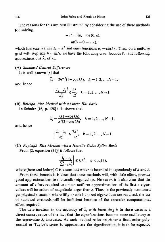
366 John Paine and Frank de Hoog [2]

The reasons for this are best illustrated by considering the use of these methodsfor solving

— u"—hi, xe(0,j[),

u(0) = 0 = u(n),

which has eigenvalues kk = k2 and eigenfunctions uk = sin kx. Then, on a uniformgrid with step size h = njN, we have the following error bounds for the followingapproximations Xk of Xk.

(A) Standard Central DifferencesIt is well known [8] that

4=2/r2(l-cosA:/0, k = \,2,...,N-\,and hence

*=:-, k = l,2,...,N-l.

(B) Raleigh-Ritz Method with a Linear Hat BasisIn Schultz [16, p. 120] it is shown that

and hence

6(1 -cos k h)V(2+cos kh)

12

(C) Rayleigh-Ritz Method with a Hermite Cubic Spline BasisFrom [2', equation (31)] it follows that

1 5 -h<ho(k),

where (here and below) C is a constant which is bounded independently of k and h.From these bounds it is clear that these methods will, with little effort, provide

good approximations to the smaller eigenvalues. However, it is also clear that theamount of effort required to obtain uniform approximations of the first n eigen-values will be orders of magnitude larger than n. Thus, in the previously mentionedgeophysical situation where fifty or one hundred eigenvalues are required, the useof standard methods will be inefficient because of the excessive computationaleffort required.

The deterioration in the accuracy of lk with increasing k in these cases is adirect consequence of the fact that the eigenfunctions become more oscillatory asthe eigenvalue Xk increases. As each method relies on either a fixed-order poly-nomial or Taylor's series to approximate the eigenfunction, it is to be expected

[3] Uniform estimation of eigenvalues 367

that the global accuracy of such approximations, and hence the eigenvalueapproximation also will deteriorate as k increases.

An alternative approach based on approximating the differential equation itselfhas been suggested by a number of authors (see, for example, [3], [7], [9], [13], [14],[15]). Specifically, we replace p, q and r in (1.1) by the approximations p, q and frespectively. Then we calculate the approximations to the eigenvalues and eigen-functions by solving

(a) -(pu')' + qu=Xru, xe(a,b),

(b) (a)0,yu(b)+5u'(b)=0, ( '

(c) u, pu'eC[a,b].

Let us neglect, for the time being, the difficulties associated with solving (1.2) andlook at some of the features of such an approach.

Potentially, for a given approximation, we can obtain estimates of all the eigen-values. It is not clear, however, whai effect these perturbations of the coefficientswill have on the eigenvalues, nor is it obvious that (1.2) will be any easier to solvethan the original problem.

In an extensive analysis of such methods, Pruess [14] has shown that for piecewiseMth order polynomial interpolation of the coefficients on a grid with maximumstepsize h,

\Xk-Xk\^ChM+l\lk\, h<h0. (1.3)

He also extends this basic result to show that for piecewise polynomial interpolationat the Gaussian points

rk\, h<ho(k), (1.4)where

For M > 0, we can see that the above bounds represent a considerable improve-ment over the bounds obtained when finite difference and variational schemes areemployed. However, in order to solve (1.2) it is necessary to obtain the fundamentalsolutions on each subinterval. If M > 0 however, there does not in general exist aclosed form for these fundamental solutions which is computationally convenient.Of course, a series solution could be developed, but this means that we are approxi-mating the fundamental solutions by means of a piecewise polynomial and this isexactly the thing we are trying to avoid. It is only when M = 0 that computationallytractable schemes can be constructed (see, for example, [3]). However, in this casewe have


for a general approximation, or if midpoint interpolation is used,

and so it is not clear that this scheme will be superior to conventional schemes.In some special situations, the above bounds have been improved. For instance,

when (1.1) is in Liouville normal form (that is, p = 1, r = 1) and q is approximatedon a uniform grid by midpoint interpolation, then Ixaru [10] has shown that

4h<h0.

Clearly, this is an improvement over the above estimates, but we still have notachieved the desired uniformity.

In this paper we use a standard perturbation argument to show that for problemsin Liouville normal form, the approximations generated by (1.2) (with p=\,r = 1) satisfy

provided \\q — q ||2 < imin* | Xk + i—?.k |. It is then shown that this bound can befurther improved for a certain class of midpoint piecewise constant approxi-mations, and a scheme is proposed which will give uniform O(h2) approximationsto all eigenvalues. Finally, we extend this method to include the uniform approxi-mation of the eigenvalues of (1.1).

2. Approximation of differential equations in normal form

In this section we restrict attention to eigenvalue problems which are inLiouville normal form

-U"+SU = )M, ueD, (2.1)

where s is a continuous function and

£> = {weL2([0,1]): u',u are absolutely continuous, U " E L 2 ( [ 0 , 1]), ocu(O) +

We further consider approximating problems of the form

- U " + S M = / U , ueD, (2.2)

where s is a piecewise continuous function.L e t U*}r=o» {4}r=o b e t h e eigenvalues of (2.1) and (2.2) respectively, arranged

in ascending order, and {uk}™=0, {«*}"=<> °e the corresponding eigenfunctions,


scaled so that

Il«*ll2 = l|fij2 = land

(uk,uk)^0.

Then we have the following results,

THEOREM 2.1. Let p =mink\Ak+1—Xk\ > 0 and s be such that \\s — s\\2 <\p-

Then,

(i) \Xk-Xk\^\\s-5h,k=O,l,2,...,

(») \\uk-uk\\2^Us-s\\2,k=0,\,2,....

PROOF, (i) The first assertion follows from a result of Kato [11, p. 291] whichstates that if T is a self-adjoint operator and B a bounded symmetric operator bothacting in a Hilbert space H, then T+B is self-adjoint, and

where 2(7) , I.(T+B) are the spectra of the operators T and T+B respectively, and

dist QA", Y] = max {sup inf | x —v| , sup inf | x — y\}xeX yeY ' yeY xeX

for any two sets X and Y contained in C.Now if we define the operators L and L by

Lu=— u"+su, ueD,Lu = —u"+su, ueD,

then it is clear that L=L — B where B is the bounded symmetric operator definedby

Bu — {s—s)u.

From [17, Theorem 10.18], L is self-adjoint and since D c: L2([0,1]), the condi-tions of Kato's theorem are satisfied and hence,

dist[Z(L),!(£)]< | |5y2.

The ordering of the spectra and the bound on || s—s\\2 then imply

I ^ - J * l < l l * - 5 | | 2 , * =0 ,1 ,2 , . . . .(ii) Let

r t = { A e C : | A - A 4 | = p } , A: =0 ,1 ,2 , . . . .

As kk and lk are the only eigenvalues of L and L respectively on the disc boundedby Tk, and both eigenvalues are interior points of Tk, the projection operators

Pk=——i) (L-kiy'dk (2.3)2niJrk


and

1 X -2ni Jrk

are well defined and

Pkf=(MkJ)«k, (2-5)

Pj=(uk,f)uk (2.6)for any/eL2([0,1]).

Furthermore, it is easily verified that for X e Tk,

and hence, from (2.6) with/=wt and (2.4),

(uk,uk)uk=Pkuk

= Pkuk+Rkuk,where

if . _ , - ! ,

That is, using (2.5) in the above,

(uk, uk) uk = uk+Rk uk. (2.7)

From Kato [11, p. 291] and the bound on ||s—s||2, we find that

I l ^ i l 2 < - | | s - s | | 2 < l (2.8)P

and, from (2.7)

But, also from (2.7),"*-"* = 0 -("k,Uk))Ok+Rkuk

and so\\uk-uk\\2^2\\Rk\\2

4

^ P

From these basic results it is also possible to derive a refined estimate of theeigenvalue perturbation which will be useful for obtaining higher order con-vergence results in the next section. This result is

THEOREM 2.2. Jf\\s — s\\2 <\p where p is as defined in Theorem 2.1, then

J oK-\~ | {s~~s)u\dx

P|


PROOF. Let A: be a given integer. From (2.7) we have, since || Rk\\2 < 1 impliesthat (uk, uk) # 0,

, "*) (2.9)

where uk and uk are the eigenfunctions of (2.1) and (2.2) respectively, correspondingto the eigenvalues Xk and lk.

Applying L to uk and using (2.2) and (2.9) yields

Luk = Xk(uk+Rk uk)l(uk, uk);

but, since L=L — B, we also have

Luk = (Xk uk - Buk + LRk uk)l(uk, uk).Hence

(4 - k) uk -Buk=-(L- lk I) Rk uk

and on taking the inner product of both sides with uk and noting that {uk, uk) = \,

Mk-2*)- (s-S)u2kdx = -(«», (L-lkI)Rkuk).

J o

But, since (L - lk I) is self-adjoint,

| (uk, ( I - lk I)Rk uk)\=\ {lk - lk) (uk, Rk uk) + (Buk, Rk uk) \

Theorem 2.1 and the inequality (2.8) then yield the desired result.

3. Convergence results for problems in normal form

From the preceding results, it is a simple matter to obtain results analogous tothose of Pruess [14] when s is approximated by a piecewise polynomial. However,due to the inherent difficulties in solving the approximate problem for the generalcase, we shall restrict attention to the case of piecewise constant approximation.

LetA = {Xi, i = 0 , 1 , . . . N\x0 = 0 , ^ = 1,

be a partition of [0,1],

h = m a x | x , + , - X i l ,

then the piecewise constant approximation s is defined by

where st is some constant.Then, from Theorem 2.1,


COROLLARY 3.1. Let seC^O, 1], A be a partition of[0,1] and Si interpolate s atsome point of[xh x,+ ii for each i. Then there is an h0 > 0 such that for each partitionA with h < h0

\*k-3*\< II*'II«A * =0 ,1 ,2 , . . . .

PROOF. If we define h0 =?pl\\s'\\x, then the result follows from Theorem 2.1

Similarly, if seC2[0, 1] and s is given by midpoint interpolation, then Ixauru's[10] result follows from Theorem 2.2, by using any standard result on the errorof midpoint product integration. However, initial computational results indicatedthat for midpoint interpolation on a uniform grid, this bound can be improved.Before giving this improved bound, the following definitions and lemmas arerequired:

LEMMA 3.1. Let {nk}™=0 and {wk}£L0 be the ordered eigenvalues and eigenfunctionsof the operator Lo, where Lo is defined by

Low = - w", WED,

and where the eigenfunctions are scaled so that

and

Then, there is a positive constant C,, bounded independently ofk, such that for eachinteger k,

(•) i K - w J L ^(ii) Hwi-wilL^

(iv) HwilL:

PROOF. All four inequalities follow directly from the asymptotic representationof the normalized eigenfunctions and their derivatives given in Courant andHilbert [6, p. 336].

On a uniform partition A of [0,1], define s* to be the piecewise constantapproximation determined by the rule

s*(x)=s(xi+i), xe(xhxi+l),where

xi+i=xt+\h, i = 0 , l , . . . , # - 1 .Then we have


LEMMA 3.2. Let seC2 [0,1], / e C1 [0,1] and A be a uniform partition of [0,1],

then

(s - s*)fdx

PROOF.

5-S*)/dx I1 = 0

N - l

Ii = 0

s'(xi+

J x,

r*t+1

J X,

+ ,S+ 1

i = O

Using the inequalities

I s(x)-s(xi+i)-s'(xi+i)(x-xi+i) I < ill s"Iand

it is easy to verify that

is — s) fax {ills'II. 11/'L+ill/"IL 11/11.}ft2-

If we now define {A*} and {u*} to be the eigenvalues and eigenfunctions of (2.2)with s = s*, then we have

THEOREM 3.1. Let seC2 [0,1], then there is an h0 > 0 such that for each uniformpartition A with h < h0,

) hmax

sin py/(rjk) hh2 + C2h

2,

k =0,1 ,2 , . . . ,

where Cl and C2 are constants bounded independently of k and h.

PROOF. Let h0 = pj\\ j 'H^.and A be a uniform partition with h < h0, then theconditions of Theorem 2.2 are satisfied since

Using the identity

uk =w2+2(uk-wk)wk+(uk-wk)2

374 John Paine and Frank de Hoog

in Theorem 2.2, we find

[10]

{s-s*)wldx +2 (s-s*)(uk-wk)wkdxJo Jo

\\ (s — s*) (uk — wk)2 dx+-llsTa,fc

2.

Estimating the last two integrals through the application of Lemma 3.2 togetherwith the bounds of Lemma 3.1, then yields

\J

(s — s*)wldx + Ch2. (3.2)

If on each of the intervals (x,,xi+1) we replace (s—s*) by a Taylor's seriesexpanded about xi+i, we obtain

(s - s*) wl dxN-l

i = 0 >J> +ih2\\s"\\oo | w*dxo

and, since wk — Aksm(yJ(rik)x+<l>k), we can integrate the above to give

fJ c

(s-s*)wldx2 1,2Alh ) h siriyj(r]k) h

N-l

s i n +ih2\\s"\\x. (3.3)

Now, on summing by parts,N - l

But since

and

N - l

) £ SIJ = O

i - 1

). (3.4)

i - l

£ s sin

(3.2), (3.3) and (3.4) give the desired result.The presence of the term

maxsin pyj(r)k) h


in the above error bound makes it immediately obvious that this bound cannotbe uniformly O(h2). In spite of this negative result, we will now show that byusing the above approach to find the first [A^/2] eigenvalues and then switchingover to a simple asymptotic expansion, uniform O(h2) estimates of all eigenvaluescan be found.

In [12] it is shown that

rsdx + Oik'2) (3.5)

and so it is clear that this expansion will provide uniform 0{h2) approximationsfor Jk = [JV/2],[JV/2] + l,. . . . Thus, we only need to show that the bound inTheorem (3.1) is uniform for A: = 0 , 1 , ...,[JV/2]. But, from [6], y/rik=thus

and so

and

Therefore,

max

) h sinyW hr,kh

2

sin py/(ijk)h

V (»/*)>>

'2y/{t,k)h

3), fc=0,l,...,[JV/2].

Consequently, the above approach does in fact yield uniform approximations toall eigenvalues.

4. Numerical schemes for piecewise constant approximation

When I is chosen as a piecewise constant function, the solution of (2.2) for agiven value of X is

A0F0{x,X) B0G0{x,X), xe[xo,xj

where F^x, X) and G((x, A) are the fundamental solutions of

> = /.i>, xe(x, ,x ( + 1)


which were chosen as

(cos QO. - Si) (x - x,)), A > s,,F,(x,A) = j l , A=s, ,

Icosh (s/(s, - A) (x - x,)), ;. < sh

sin (N/(A - Sj) (x - Xi))/y/(/. - s(), A > sh

G,(x, /.) = (x — x,), /, ^ s-sinh (^/(s, - A) (x - x,))/^(s,. - A), A < sf.

The constants {>!,•, B,}f=0' are determined up to an arbitrary multiple by theadditional requirement that vxeD.

The determination of the eigenvalues of (2.2) thus becomes that of finding thevalues of A for which {A^JQ and {B^JQ are not identically zero. To do this, wenote that the requirement vxeD yields a system of equations involving theunknowns Ah Bh vx(x,), D/(X;) and the known values F,(xI+1,A), and G;(xi+1,A).We can then proceed in a number of ways, for example, Canosa [3] uses theserelations to eliminate the unknowns {vx(Xj), ^ (x , )}^ 1 and obtains a system ofequations in {At, B.jfLV- The eigenvalues are then simply the zeros of the deter-minant of this system. However, if these relations are used to eliminate theunknowns {Ah B;}f=V and { .'(x,)}^",,1 from the continuity conditions, we obtainGt+\(Xi + 2> V Vx(x,)-[Fi(xi+1,A)Gi+ i(xi + 2, A)+/"i+ !(xi + 2 , A)Gf(xi+ u A)] vx(xi+1)

+ Gi(xi+Ul)vx(xi+2)=O, i = 0,l,...,N-2.These relations, together with the equations

xu A)-«C0(x1, A)] v1ix0)-Pvx(xl)=0and

-Svx(xN_1) + [_yGN_1(xN, X)+dFN_ ,(xN, A)] vx(xN) = 0

which are obtained in a similar fashion from the boundary conditions, yield asystem of equations of the form

where

vT = (vx(x0), vx{,x,),..., vx(xN))

and D{1) is a tridiagonal matrix.This approach provides a simpler procedure for finding the eigenvalues of (2.2)

and also yields a simple direct method for evaluating the eigenfunction at the knotsof the partition. Unfortunately, there is the difficulty that not all zeros of thedeterminant are necessarily eigenvalues. To illustrate this, consider the problem

-V" =AV,

the exact eigenvalues of which are A* = {k+\)2, k=0,\,2

[13] Uniform estimation of eigenvalues

Now for the partition {0, \n, n)

377

cos - 1

•sin2—sin

2

0

cos- —r-sin •^ 2

and so,det(ZXA)) = - — sin 2^M? cos J(A) jr.

N/A 2

Therefore det(D(A)) is zero whenever A is an eigenvalue, but it is also zero whenA = 4p2, p = 1,2,..., which are not eigenvalues.

Although there does not appear to be any simple analytical means for removingthese extraneous zeros, it should be noted that they are an artefact introduced bythe elimination of the values {v'x(xi)}fjo

l and that they only arise non-triviallywhen G((xl+1, A) and G( + 1(xi + 2 , A) both vanish for some value of A. This can onlyoccur when A ^ n2jh2 — \\ s \\K. Thus, for most problems this difficulty either willnot occur or will occur in a range for which the asymptotic expansion rather thanthe approximation method will be used.

5. Approximation of differential equations not in normal form

Although the technique of approximating the coefficients of the differentialequation by piecewise constant functions provides a uniform approximation to theeigenvalues when the problem is in normal form, it can be shown that when thistechnique is applied to (1.1), Pruess' estimates (1.3) and (1.4) are sharp.

This suggests that when the problem is not in normal form, we should use theLiouville transformation to transform (1.1) into normal form. Thus if

p,q,reC\_a,b\ pr^O and preC\a,b\

then the Liouville transformation

= T"X \\rlpfdx, T = P(rlp)*dx,

u=wz, w=transforms (1.1) to

where

and

-z+sz=vz, te(0,1),

s(t) = T2(qlr)(t)-(wM(0+2(wlw)2(t)

v=T2L

(5.1)

(5.2)

(5.3)

(5.4)


Similarly the boundary conditions become

«*z(O)+j8z(O)=O,

y*z(l)+<5i(l)=0, (5.5)where

«*=and

We can then use the previously outlined method to obtain uniform approxi-mations to the eigenvalues of this transformed problem and hence of the originalproblem. In some cases, however, it may not be possible to carry out this trans-formation explicitly. Thus, to obtain uniform approximations, it becomes necessaryto introduce a further approximation.

From the form of the exactly transformed problem, it can be seen that thetransformation parameter T, the function 5 and the boundary condition coefficientsa* and y* all need to be approximated. Let us therefore consider how we shouldperform these approximations:

From Theorem 2.1 it is clear that an O(e) perturbation of s will produce, at most,an 0(e) perturbation of the eigenvalues. Thus if s(t) cannot be evaluated exactly,it is a relatively simple matter to approximate the desired quantities with sufficientaccuracy so that the order of approximation of the eigenvalues is not affected.

The approximation of the parameter T, however, poses a more severe problem,since it is clear from (5.4) that a perturbation of T will produce a perturbation inthe eigenvalues which is proportional to the size of the eigenvalue. In practice,however, T may be evaluated with sufficient accuracy so that any non-uniformitywill not be apparent in the range of eigenvalues which are of interest.

The final problem is the effect of perturbations in a* and y*. If these valuescannot be found exactly, the conditions of Kato's theorem are no longer satisfied.We overcome this problem with

THEOREM 5.1. Let {Xk(o, r\)}^=0 be the ordered eigenvalues and {uk(u,a,t])}^0 bethe corresponding normalized eigenfunctions of

-U" + SU=)M, xe(0,1),

(Tu(0)-u'(0)=0.

where seC[0,1]. Then

where M is independent ofk.

do dr,


PROOF. It is clearly sufficient to show that the derivatives of lk{a, ri) with respectto a and 77 exist and are continuous. To do this we note that At(a, r]) is a continuousfunction of a and rj [6, p. 419] and also that uk(x, a, rf) depends continuously ona and r] [4, p. 58].

Let u(x) — uk(x, ff, tj) and u(x) = uk(x, <x,fj), then

— u" + su =Xk(<r,t])uand

— u" + su = Xk(d,r\)u.Therefore

\_Xk{a, rj) -Afc(a,fj)] w« = - u"u + uu" (5.6)

and, on noting that

*i

J o(-u"u + uu")dx = [-u'

we find on integrating (5.6),

fl). (5.7)7,i)-Ak(d,f\)']J 00

Now, since uk depends continuously on a and rj, there is a <5 = ^(/c) such that

J ouu dx > 0

whenever (<7,fj)sA (o-,>7) = {(x,y): (x — a)2+(y — rj)2 < <52}. Hence, from (5.7),

whenever (i?,f|) e ^(tx, >/).

On taking the relevant limits and noting that

P= lim uudx = |d=a,ij-*rjJo

lim uudx= lim uudx = \\ uk | | | = 1,a-* a, fj~t} J 0 d =tr, ij—>^J 0

we find that the derivatives of Xk with respect to a and ^ exist, and

and

Thus the derivatives are continuous and bounded by [| w H . The result thenfollows from the eigenfunction bounds in Lemma 3.1.


Using these bounds in a standard mean value theorem shows that the per-turbation of the eigenvalues is of the same order as the perturbations in a* andy*. Thus, if a* and y* are approximated sufficiently well, the desired properties ofthe eigenvalue approximations will not be lost.

6. Numerical examples

To provide numerical confirmation of the preceding results, the method basedon the three-term recurrence relation and outlined in Section 4 was implementedin a computer program. The determinant of the matrix was evaluated usingGaussian elimination with partial pivoting. The zeros were found using a modifiedsecant method, the initial values for which were found by a fixed step search basedon an initial prediction provided by an asymptotic expansion for the eigenvalues.

The first problem considered was

?M, te(0,1),

M(0)=0=ii(l).

The approximating problem was chosen to be that given by approximating s usinga midpoint approximation rule on a uniform partition with N intervals.

The first forty eigenvalues of this approximating problem for TV =16 werefound, and an estimate of the error was obtained by comparing these results with

en

M O " 3

enen

6

4

2

.0

.0

.0

.0

- XTxxxxxxxxxxxx

- 2 - 0

- 4 . 0

- 6 . 0

X

i i i i 1 i i i i I i i i i i i i i i5

Iio

i15

I I I I25 30 4 0

x

x

EIGENVRLUE NUMBER

Fig. 1. Eigenvalue error for problem I.

117] Uniform estimation of eigenvalues 381

those obtained for N = 256. The errors thus obtained are plotted in Fig. 1, and itshould be noted that they appear to be in close agreement with the bound givenin Theorem 3.1.

At this stage it is worthwhile pointing out that for this example, the O(h) peaksare in apparent disagreement with the asymptotic formula equation (42) of [14]which predicts that the error in this example should decrease like O(k~2). How-ever, the observation that this asymptotic formula requires s and s to be con-tinuously differentiate resolves this contradiction since this condition is clearlynot satisfied by piecewise constant approximations.

From the above figure and comments it is clear this method will not directlyyield the desired uniform approximations and so the strategy of switching to theasymptotic expansion (3.5) will have to be used. The error in the approximationsobtained in this manner for the above example (again with N =\6)is presented inFig. 2 and clearly shows that this is a viable strategy for obtaining uniformapproximations.

LJ

8 . 0

7 . 0

6 . 0

5 . 0

4 0^ "u

3.0

2.0

1 .0

.0

1 .0

:xx X

XX

XX X

X

< X x * x x x x xXXXXXXXXXXXX)

I I I I I I I I I I I I I I I I I I I I I I I I I I I I I I I I I I I I I I I10 15 20 25 30 35 40

EIGENVflLUE NUMBERFig. 2. Eigenvalue error using approximation of differential equation and asymptotic expansion

for problem I.

The next problem considered was

x x

382 John Paine and Frank de Hoog [18)

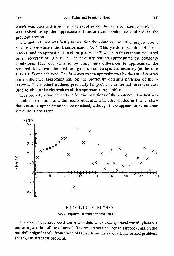
which was obtained from the first problem via the transformation x = e1. Thiswas solved using the approximate transformation technique outlined in theprevious section.

The method used was firstly to partition the x-interval, and then use Simpson'srule to approximate the transformation (5.1). This yields a partition of the /-interval and an approximation of the parameter T, which in this case was evaluatedto an accuracy of 1.0 x 10~6. The next step was to approximate the boundaryconditions. This was. achieved by using finite differences to approximate therequired derivatives, the mesh being refined until a specified accuracy (in this case1.0 x 10~4) was achieved. The final step was to approximate s by the use of centredfinite difference approximations on the previously obtained partition of the t-interval. The method outlined previously for problems in normal form was thenused to obtain the eigenvalues of this approximating problem.

This procedure was carried out for two partitions of the x-interval. The first wasa uniform partition, and the results obtained, which are plotted in Fig. 3, showthat accurate approximations are obtained, although there appears to be no clearstructure in the error.

CD

a:

5.0

4.0

3.0

2.0

1 .0

.0

-1 .0

-2 .0

x x

x

xxx x

X X

X

X

X X

XX

X X

I I I 1 I I I I I I 1 I I I 1 1 1 I I I I I I I I I I I I I I I I J ; l I I I I IL 5 1 0 r5 20 25 30 35 40

EIGENVRLUE NUMBERFig. 3. Eigenvalue error for problem II.

The second partition used was one which, when exactly transformed, yielded auniform partition of the /-interval. The results obtained for this approximation didnot differ significantly from those obtained from the exactly transformed problem,that is, the first test problem.


References

[1] R. S. Anderssen and J. R. Cleary, "Asymptotic structure in torsional free oscillations of theearth—I. Overtone structure", Ceophys. J.R. Astr. Soc. 39 (1974), 241-268.

[2] G. Birkhoff, C. de Boor, B. Swartz and B. Wendroff, "Rayleigh-Ritz approximation bypiecewise cubic polynomials", SIAM J. Numer. Anal. 3 (1966), 188-203.

[3] J. Canosa and R. G. de Oliveira, "A new method for the solution of the Schrodingerequation", J. Comp. Phys. 5 (1970), 188-207.

[4] E. Coddington and N. Levinson, Theory of ordinary differential equations (McGraw-Hill,New York, 1955).

[5] S. D. Conte and C. de Boor, Elementary numerical analysis: an algorithmic approach(McGraw-Hill, New York, 1972).

[6] R. Courant and D. Hilbert, Methods of mathematical physics, Vol. I (Interscience, New York,1953).

[7] R. Gordon, "New method for constructing wave functions for bound states and scattering",J. Chem. Phys. 51 (1969), 14-25.

[8] R. T. Gregory and D. T. Karney, A collection of matrices for testing computational algorithms(Wiley-Interscience, New York, 1969).

[9] N. A. Haskell, "The dispersion of surface waves on multilayered media", Bull. Seismol. Soc.Amer. 43 (1953), 17-34.

[10] L. Gr. Ixaru, "The error analysis of the algebraic method for solving the Schrodingerequation", J. Comp. Phys. 9 (1972), 159-163.

[11] T. Kato, Perturbation theory for linear operators (Springer-Verlag, Berlin, 1966).[12] M. R. Osborne, "Numerical procedures for the eigenvalue problems of second order ordinary

differential equations when a wide range of eigenvalues are required". In Adas delseminario sobre metodos numericos modernos, Vol. II (Caracas, 1974).

[13] M. R. Osborne and S. Michaelson, "The numerical solution of eigenvalue problems in whichthe eigenvalue parameter appears non-linearly, with an application to differentialequations", Computer J. 1 (1964), 66-71.

[14] S. Pruess, "Estimating the eigenvalues of Sturm-Liouville problems by approximating thedifferential equation", SIAM J. Numer. Anal. 10 (1973), 55-68.

[15] S. Pruess, "High order approximations to Sturm-Liouville eigenvalues", Numer. Math. 24(1975), 241-247.

[16] M. H. Schultz, Spline analysis (Prentice Hall, Englewood Cliffs, N.J., 1973).[17] M. H. Stone, Linear transformations in Hilbert space (American Mathematical Society,

New York, 1932).[18] C. Wang, J. F. Gettrust and J. R. Cleary, "Asymptotic overtone structure in eigenfrequencies

of torsional normal modes of the earth: a model study", Geophys. J.R. Astr. Soc. 50(1977), 289-302.

Computing Research GroupAustralian National UniversityP.O. Box 4, Canberra, A.C.T. 2600AustraliaandC.S.I.R.O. Division of Mathematics and StatisticsYarralumla, A.C.T. 2600Australia

Uniform estimation of the eigenvalues of Sturm–Liouville problems

Documents

Transcript of Uniform estimation of the eigenvalues of Sturm–Liouville problems