2 Direction Solution of Linear Equations

25

Chapter 2. Direct Solution of Linear Equations

Sets of simultaneous equations arise in a large number of mathematical and engineering applications.

Examples include:

Finite difference methods. These will be covered later in the course and are used to model a wide

variety of physical phenomena such as heat flow, vibrating structures, magnetic fields and

groundwater flow.

Finite element methods. Finite element analysis is extensively used in Civil, Environmental,

Mechanical and Electrical Engineering. The technique can be used to solve almost any set of

differential equations.

Least squares fitting.

In many cases, very large systems of equations need to be solved. For example, in the aircraft and

construction industries it is not uncommon for finite element analysis to generate systems of equations

with several hundred thousand unknowns. In order to solve large systems efficiently, a number of

ingenious algorithms have been developed. These usually exploit any special features that the

equations may have.

The system of linear equations to be solved may be written in the form

11 1 12 2 1 1

21 22 2 2 2

1 1 2 2

n n

n n

n n nn n n

a x a x a x b

a x a x a x b

a x a x a x b

In matrix notation, this becomes

A x = b (2.1)

where

11 12 1 1 1

21 22 2 2 2

1 2

1 1

n

n

n n nn n n

a a a x b

a a a x b

a a a x b

n n n n

A x b

The matrix A is defined to be square if the number of rows is equal to the number of columns. Most

sets of linear equations that arise in engineering applications involve square matrices. Square matrices

often display characteristics that enable them to be classified into certain groups. Some important

categories are listed below:

A matrix is lower triangular if all of the coefficients above the diagonal are zero, as shown in

Figure 2.1. Lower triangular matrices are important in linear equation solution algorithms, and

will be discussed subsequently.

0 0

0

x

x x

x x x

x = nonzero coefficient

Figure 2.1: Lower triangular matrix

26

A matrix is upper triangular if all of the coefficients below the diagonal are zero, as shown in

Figure 2.2. Upper triangular matrices are also important in equation solution algorithms,

especially Gauss elimination.

0

0 0

x x x

x x

x


Figure 2.2: Upper triangular matrix

A matrix is said to be diagonal if all the coefficients, except those on the diagonal, are zero. An

example of a diagonal matrix is shown in Figure 2.3.

0 0

0 0

0 0

x

x

x


Figure 2.3: Diagonal matrix

A matrix is said to be tridiagonal if all the nonzero coefficients lie on the superdiagonal, the

diagonal, and the subdiagonal. More formally, a tridiagonal matrix has 0ija whenever

1.i j A tridiagonal matrix is shown in Figure 2.4. This type of structure occurs frequently in

the solution of partial differential equations, and can be solved very efficiently using a special

algorithm which will be discussed later in this section.

Figure 2.4: Tridiagonal matrix

A diagonally dominant matrix is one which has large entries on its diagonal. More specifically,

the diagonal entries iia satisfy the relation

11

for 1,2,...,n

ii ij

jj

a a i n

The matrix shown in Figure 2.6 is diagonally dominant since the above condition is obeyed for

each row. If the condition is violated for any one of the rows, the matrix is not diagonally

dominant.

27

5 1 2 1

1 3 1 0

1 0 2 0

0 0 0 1

Figure 2.6: Diagonally dominant matrix

Diagonally dominant matrices arise in a finite difference models and will be encountered later in

the course. They have important properties that make their linear equations easy to solve using a

number of different algorithms.

A positive definite matrix is one which satisfies the relation

T > 0x A x

where T

1 2, , ... , nx x xx is an arbitrary vector which is the transpose (T) of x. Positive

definite matrices arise in least squares fitting and are also common in many finite element

applications. They have important properties which enable very efficient algorithms to be used to

solve their corresponding linear equations. A positive definite matrix is not easy to identify, but it

must satisfy the following conditions:

The diagonal entries are all positive, so that

0 for 1,2,...,iia i n

The absolute value of the largest entry on the diagonal is not less than the absolute value of the

largest entry anywhere else in the matrix. Mathematically, this condition can be expressed as:

1 , 1

max maxjk iij k n i nj k

a a

For each entry in the matrix 2 forij ii jja a a i j

An example of a positive definite matrix is shown in Figure 2.7.

1 1 0 0

1 2 1 0

0 1 2 1

0 0 1 1

Figure 2.7: Positive definite matrix

2.1 Direct and Iterative Methods for Solving Linear Equations

There are two types of approaches for solving sets of linear equations. These are:

28

Iterative methods. These start with an initial guess for the solution and iteratively improve this

until the equations are satisfied. The number of iterations involved is often difficult to assess, as it

depends on the iteration method and the type of the matrix equations. Convergence can be

guaranteed for some algorithms, however, when they are applied to certain types of matrices. This

will be discussed in more detail in the next Section.

Direct methods. These are distinct from iterative methods in that the solution is obtained using a

single sweep with a finite (and predictable) number of operations. This class of schemes will be

discussed exclusively in this section.

With either type of method, we rarely get the exact solution due to the effects of roundoff error which

is caused by finite precision arithmetic. It is most important that any algorithm is able to detect when

the linear equations has no solution. This case is often difficult to predict by inspection for very large

systems.

2.2 Gauss Elimination

Gauss elimination is a direct method for solving systems of linear equations. The basic idea behind the

method is to operate on the equations (2.1) to produce equivalent upper triangular system of the form

U x = c (2.2)

where

11 12 1 1 1

22 2 2 2

1 1

0

0 0

n

n

nn n n

n n n n

u u u x b

u u x c

u x c

U x c

The operations necessary to produce (2.2) are known as factorisation steps. To explain the Gauss

factorisation procedure, consider the system of three linear equations shown below

11 12 13 1 1

21 22 23 2 2

31 32 33 3 3

a a a x b

a a a x b

a a a x b

Multiplying the first equation by 21 11a a (assuming that 11 0a ) and subtracting from the second

produces the equivalent system

11 12 13 11

2 2 2

22 23 2 2

31 32 33 3 3

0

a a a bx

a a x b

a a a x b

where the superscript (2) denotes iteration number and

2

22 22 21 11 12

2

23 23 21 11 13

2

2 2 21 11 1

a a a a a

a a a a a

b b a a b

(2.3)

29

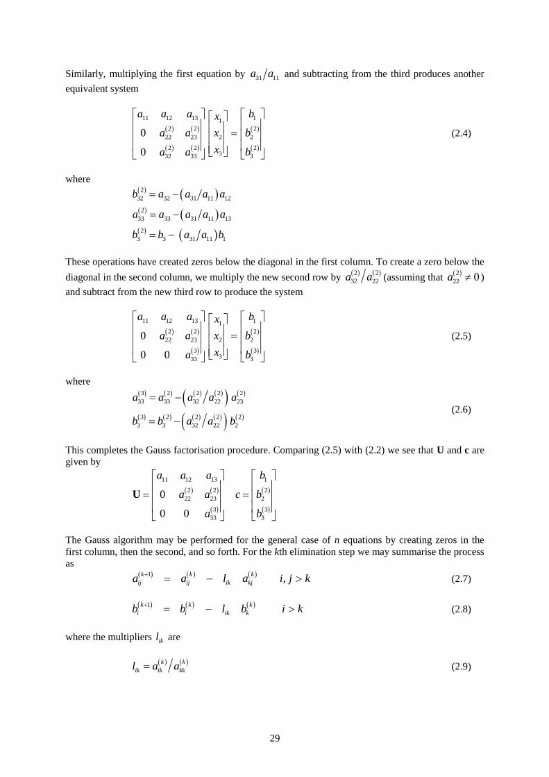
Similarly, multiplying the first equation by 31 11a a and subtracting from the third produces another

equivalent system

11 12 13 11

2 2 2

22 23 2 2

2 2 2332 33 3

0

0

a a a bx

a a x b

xa a b

(2.4)

where

2

32 32 31 11 12

2

33 33 31 11 13

2

3 3 31 11 1

b a a a a

a a a a a

b b a a b

These operations have created zeros below the diagonal in the first column. To create a zero below the

diagonal in the second column, we multiply the new second row by 2 2

32 22a a (assuming that 2

22 0a )

and subtract from the new third row to produce the system

11 12 13 11

2 2 2

22 23 2 2

3 3333 3

0

0 0

a a a bx

a a x b

xa b

(2.5)

where

3 2 2 2 2

33 33 32 22 23

3 2 2 2 2

3 3 32 22 2

a a a a a

b b a a b

(2.6)

This completes the Gauss factorisation procedure. Comparing (2.5) with (2.2) we see that U and c are

given by

11 12 13 1

2 2 2

22 23 2

3 3

33 3

0

0 0

a a a b

a a c b

a b

U

The Gauss algorithm may be performed for the general case of n equations by creating zeros in the

first column, then the second, and so forth. For the kth elimination step we may summarise the process

as

1

,k k k

ij ij ik kja a l a i j k

(2.7)

1k k k

i i ik kb b l b i k

(2.8)

where the multipliers ikl are

k k

ik ik kkl a a (2.9)

30

and k = 1,2,….,n – 1, 1

and , 1,2,..., .ij ija a i j n In order for the Gauss procedure to succeed, the

condition that

0k

kka must hold for all k = 1,2,….,n. These entries are called pivots in Gaussian

elimination.

Once the equations are in the upper triangular form of (2.2), the solution can be obtained by back-

substitution. This process starts with the last modified equation and works backwards, with the

unknowns being found in reverse order. To see how back-substitution works, consider the triangular

system (2.5) which may be written as

11 12 13 1 1

22 23 2 2

33 3 3

0

0 0

u u u x c

u u x c

u x c

The third equation gives

33 3 3u x c

Provided 33 0u , this gives 3x by simple division as

3 3 33x c u

Now using the second equation, we have

22 2 23 3 2u x u x c

which (for 22 0u ) furnishes 2x as

2 2 23 3 22x c u x u

Finally, from the first equation

11 1 12 2 13 3 1u x u x u x c

which (for 11 0u ) gives 1x as

1 1 12 2 13 3 11x c u x u x u

The back-substitution process may clearly be generalised to a system of n equations and may be

summarised by the relations

n n nnx c u (2.10)

1

for 1,...,2,1n

k k kj j kk

j k

x c u x u k n

(2.11)

The back-substitution process is well defined provided that 0kku for all 1,2,..., .k n This

condition is automatically satisfied if none of the pivots are zero during the elimination phase.

31

To illustrate the Gauss elimination algorithm, consider the system of linear equations shown below

1

2

3

3 1 2 12

1 2 3 11

2 2 1 2

x

x

x

(2.12)

Applying the steps shown in (2.7) and (2.8), we obtain the three entries in the new row 2 as

2 1 1 1 1

2 2 21 11 1

2 1 1 1 1

2 2 21 11 1

11 2 3 3 1 2

3

0 7 3 7 3

111 12

3

7

j j ja a a a a

b b a a b

and the new row 3 as

2 1 1 1 1

3 3 31 11 1

2 1 1 1 1

3 3 31 11 1

22 2 1 3 1 2

3

0 4 3 7 3

22 12

3

6

j j ja a a a a

b b a a b

This gives the modified set of equations

1

7 723 3

7433 3

3 1 2 12

0 7

0 6

x

x

x

Note that the first row is unchanged and that zeros have been created below the diagonal in the first

column. Applying (2.7) and (2.8) again, with k=2, we obtain yet another row 3 as

3 2 2 2 1

3 3 32 22 2

3 2 2 2 2

3 3 32 22 2

40 4 3 7 3 0 7 3 7 3

7

0 0 1

46

7

2

j j ja a a a a

b b a a b

32

This completes the elimination phase as the matrix equations are now in the upper triangular form

U x = c

where

7 73 3

3 1 2 12

0 7

0 0 1 2

U c

The solution can now be obtained using back-substitution. Applying (2.10) gives

3 3 33 2/ 1 2x c u

Using equation (2.11) furnishes the remaining unknowns according to

3

2 2 2 22

3

2 23 3 22

77 2 7 3

3

1

j j

j

x c u x u

c u x u

3

1 1 1 11

2

1 12 2 13 3 11

12 2 1 2 2 3

3

j j

j

x c u x u

c u x u x u

2.3 Gauss Elimination with Row Interchanges

Consider a set of three linear equations which, after elimination of the first column, produces the

system

11 12 13 11

2 2

23 2 2

2 2 2332 33 3

0 0

0

a a a bx

a x b

xa a b

This simply corresponds to (2.4) with 2

22 0a and, from (2.3), will always happen if the original

coefficients are refined so that 22 21 11 12.a a a a If we attempt to make 2

32 0a using equation

(2.6), an error will occur when we attempt to divide by the pivot 2

22 0a . To allow for this case, we

scan down the current elimination column, starting from immediately below the diagonal, and locate

the first entry which is nonzero. The row holding this entry is then exchanged with the current pivot

row. In the above example, rows two and three would be exchanged to give

33

11 12 13 11

2 2 2

32 33 2 3

2 2323 2

0

0 0

a a a bx

a a x b

xa b

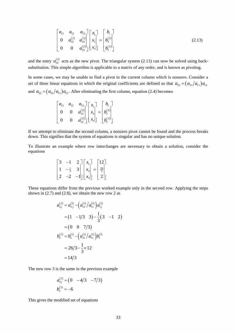
(2.13)

and the entry 2

32a acts as the new pivot. The triangular system (2.13) can now be solved using back-

substitution. This simple algorithm is applicable to a matrix of any order, and is known as pivoting.

In some cases, we may be unable to find a pivot in the current column which is nonzero. Consider a

set of three linear equations in which the original coefficients are defined so that 22 21 11 12a a a a

and 32 31 11 12a a a a . After eliminating the first column, equation (2.4) becomes

11 12 13 11

2 2

23 2 2

2 2333 3

0 0

0 0

a a a bx

a x b

xa b

If we attempt to eliminate the second column, a nonzero pivot cannot be found and the process breaks

down. This signifies that the system of equations is singular and has no unique solution.

To illustrate an example where row interchanges are necessary to obtain a solution, consider the

equations

1

26123 3

3

3 1 2 12

1 3

2 2 1 2

x

x

x

These equations differ from the previous worked example only in the second row. Applying the steps

shown in (2.7) and (2.8), we obtain the new row 2 as

2 1 1 1 1

2 2 21 11 1

2 1 1 1 1

2 2 21 11 1

11 1 3 3 3 1 2

3

0 0 7 3

126 3 12

3

14 3

j j ja a a a a

b b a a b

The new row 3 is the same in the previous example

2

3

2

3

0 4 3 7 3

6

ja

b

This gives the modified set of equations

34

1

7 1423 3

7433 3

3 1 2 12

0 0

0 6

x

x

x

Problems now arise with the next elimination step as the next pivot, on the second diagonal position, is

zero. In this case, a row interchange is necessary before proceeding further. We now scan down the

second column, starting from just below the diagonal, and look for a nonzero entry. Since row 3 has

nonzero entry in its second column, this becomes the new pivot row. Rows 2 and 3 are then swapped

to give

1

7423 3

7 1433 3

3 1 2 12

0 6

0 0

x

x

x

This set of matrix equations is in upper triangular form and there is no need to perform the last

elimination step (the step can still be executed but the equations will remain unchanged). Using back

substitution, the solution is

3

2

1

14 3 7 3 2

76 2 4 3 1

3

12 1 1 2 2 3 3

x

x

x

2.4 Singular Equations and Linear Dependence

Some sets of equations do not have a unique solution and are said to be singular. Singularity is

detected in our Gauss elimination algorithm by a zero (or near-zero) pivot, and may take several

forms. Consider the matrix equations

1

2

3

1 2 3 5

2 4 1 7

1 14 11 2

x

x

x

(2.14)

Even though this system is only of rank 3, it is not obvious whether it has a solution or not. Applying

Gauss elimination yields the upper triangular form

1

2

3

1 2 3 5

0 8 7 3

0 0 0 1

x

x

x

Because the third pivot is equal to zero, this system is singular. More precisely, the system is said to be

inconsistent since the last equation gives

30 1x

which clearly has no solution. To illustrate another type of singularity, consider the matrix equations

35

1

2

3

1 2 3 5

2 4 1 7

1 14 11 1

x

x

x

(2.15)

These are identical to the previous equations except for the third entry on the right hand side. Applying

Gauss elimination again we obtain

1

2

3

1 2 3 5

0 8 7 3

0 0 0 0

x

x

x

Because the third pivot is again equal to zero, Gauss elimination will report that the system is singular.

Expanding the last equation gives

30 0x

Clearly this has an infinite number of solutions and the system is said to be redundant. The infinite

number of solutions are

3

2 3

1 2 3

arbitary

13 7

8

5 2 3

x

x x

x x x

Another method of checking whether the coefficient matrix A is singular is to use the concept of linear

dependence. Consider a set of arbitrary vectors, 1 2, ,..., nv v v which are all of the same length. These

vectors are said to be linearly dependent if we can find coefficients 1 2, ,..., n (with not all of the

i simultaneously zero) such that

1 1 2 2 ... n n v v v 0 (2.16)

For the matrix of coefficients in (2.14) and (2.15), let the first, second and third columns be denoted,

respectively, by the vectors 1 2, and nv v v . Equation (2.16) then becomes

1 2 3

1 2 3 0

2 4 1 0

1 14 11 0

which can be expressed as the matrix equation

1

2

3

1 2 3 0

2 4 1 0

1 14 11 0

a

a

a

Performing Gauss elimination on this system gives the infinite set of solutions

36

3

2 3

1 2 3

arbitrary

7

8

2 3

a

a a

Choosing 3 8, for example, gives 2 17 and 10 and we see that

1 2 310 7 8 v v v 0

Thus, the matrix of coefficients in (2.14) and (2.15) has linearly dependent columns and the equations

do not have a unique solution

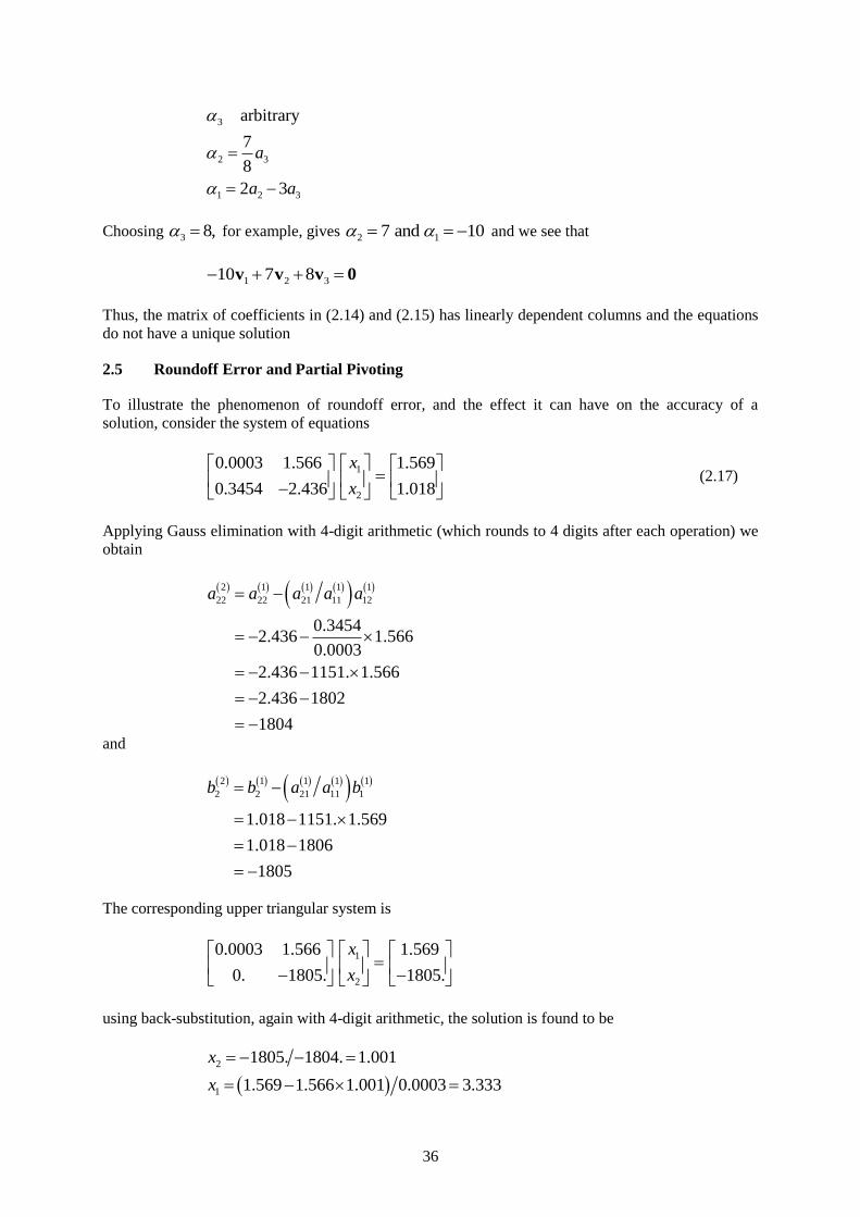
2.5 Roundoff Error and Partial Pivoting

To illustrate the phenomenon of roundoff error, and the effect it can have on the accuracy of a

solution, consider the system of equations

1

2

0.0003 1.566 1.569

0.3454 2.436 1.018

x

x

(2.17)

Applying Gauss elimination with 4-digit arithmetic (which rounds to 4 digits after each operation) we

obtain

2 1 1 1 1

22 22 21 11 12

0.34542.436 1.566

0.0003

2.436 1151. 1.566

2.436 1802

1804

a a a a a

and

2 1 1 1 1

2 2 21 11 1

1.018 1151. 1.569

1.018 1806

1805

b b a a b

The corresponding upper triangular system is

1

2

0.0003 1.566 1.569

0. 1805. 1805.

x

x

using back-substitution, again with 4-digit arithmetic, the solution is found to be

2

1

1805. 1804. 1.001

1.569 1.566 1.001 0.0003 3.333

x

x

37

or

3.333

1.001

x

This is dramatically different from the exact solution

10

1exact

x

In this case, the elimination process is very sensitive to roundoff error and the stability of the Gauss

scheme is unsatisfactory. One obvious answer to this difficulty is to use higher precision in the

calculations. With large systems of equations, however, this strategy is often of limited use. A better

approach is to identify the cause and find a cure by using a different algorithm.

Inspection of the elimination process indicates that the problem is caused the first pivot, 1

11 0.0003,a which is too small to be used as a divisor. In general, division by small numbers leads

to a loss of accuracy and should be avoided if possible. This immediately suggests the use of row

interchanges, where the pivot row is chosen to given the pivot with the largest magnitude and is a

simple extension of the idea that we used in Gauss elimination, where the pivots were chosen by

searching each column for a nonzero entry. Applying this idea to equations (2.17), we note that row 2

has the largest entry in column 1 and thus rows 2 and 1 arte interchanged prior to doing the

elimination step. This gives

1

2

0.3454 2.436 1.108

0.0003 1.566 1.569

x

x

After elimination with 4-digit arithmetic, we obtain

2 1 1 1 1

22 22 21 11 12

0.00031.566 2.436

0.3454

1.566 0.0009 2.436

1.566 0.0022

1.568

a a a a a

and

2 1 1 1 1

2 2 21 11 1

1.569 0.0009 1.018

1.569 0.0009

1.568

b b a a b

so that the corresponding upper triangular system is

38

1

2

0.3454 2.436 1.108

0. 1.568 1.568

x

x

Using 4-digit back-substitution, the solution is found to be

2

1

1.568 1.568 1.000

1.018 2.436 1.000 0.3454 10.00

x

x

which is exact to four digits. The algorithm just described is known as Gauss elimination with partial

pivoting (it is also called maximum column pivoting). Another type of strategy, which is called full

pivoting, can also be used. This is much more complicated than partial pivoting, since it involves a

scan of all the unreduced equations during each elimination step, together with row and column

interchanges.

To illustrate the partial pivoting scheme on a larger problem, consider the system of equations

1

2

3

1 2 3 11

2 2 1 2

3 1 2 12

x

x

x

(2.18)

Scanning column 1, from the diagonal down, we see that row 3 has the largest entry for a potential

pivot. Thus, before doing the first elimination step, we interchange rows 1 and 3 to give

1

2

3

3 1 2 12

2 2 1 2

1 2 3 11

x

x

x

Applying the steps shown in (2.7) and (2.8), we obtain the new row 2 as

2

2

2

2

22 2 1 3 1 2

3

0 4 3 7 3

22 12

3

6

ja

b

and the new row 3 as

2

3

2

3

11 2 3 3 1 2

3

0 7 3 7 3

111 12

3

7

ja

b

Thus, after the first elimination step, we have

39

1

7423 3

7 733 3

3 1 2 12

0 6

0 7

x

x

x

Scanning column 2, from the diagonal down, we see that row 3 has the largest entry for a potential

pivot. Prior to doing the second elimination step, we interchange rows 2 and 3 to give

1

7 723 3

7433 3

3 1 2 12

0 7

0 6

x

x

x

After applying the elimination steps we obtain the new row 3 as

3

3

2

2

40 4 3 7 3 0 7 3 7 3

7

0 0 1

46 7

7

2

ja

b

and the upper triangular system

1

7 723 3

3

3 1 2 12

0 7

0 0 1 2

x

x

x

Using back-substitution, the solution is

3

2

1

2 1 2

77 2 7 3 1

3

12 1 1 2 2 3 3

x

x

x

2.6 LU Factorisation

Gauss elimination can be interpreted in another way which leads to an alternative method for solving

sets of linear equations. The method hinges on the fact that we can express any non-singular matrix A

as a product of a lower triangular matrix L and an upper triangular matrix U according to

=A L U

Strictly speaking, the above form is true only if the Gaussian upper triangular matrix U can be found

without the need for row interchanges. A very similar expression holds, however, if row interchanges

are permitted and this will be discussed later. The matrices L and U are called the LU factors, and the

process of computing them is known as LU factorisation.

40

To illustrate an LU factorisation, let us reconsider the matrix equations (2.12)

1

2

3

3 1 2 12

1 2 3 11

2 2 1 2

x

x

x

(2.19)

Applying Gauss elimination produced the upper triangular matrix

7 73 3

3 1 2

0

0 0 1

U (2.20)

The lower triangular matrix L is constructed by storing the row multipliers, defined by equation (2.9),

for each elimination step. With reference to the previous working for the above example, the

multipliers for rows 2 and 3 in the elimination of column 1 were 1 3 and 2 3 respectively. This gives

21 311 3 and 2 3l l . Similarly, the multiplier for row 3 in the elimination of column 2 was

4 7 so that 32 4 7.l Using the additional condition that the diagonal entries of L are always

unity, we obtain

13

2 43 7

1 0 0

1 0

1

L (2.21)

Now, multiplying (2.20) by (2.21) we see that

7 713 3 3

2 43 7

1 0 0 3 1 2

1 0 0

1 0 0 1

3 1 2

1 2 3

2 2 1

L U

A

(2.22)

as required. A key feature of this type of factorisation is that it can be stored in compact form. By this

we mean that the original matrix A can be over-written by L and U without the need for additional

storage. For example, the final factorisation shown in equation (2.22) can be stored as

7 713 3 3

2 43 7

3 1 2

1

L U

There is no need to store the diagonal terms of the L matrix as they are known to be equal to unity.

Once the L and U matrices have been computed, the original set of equations Ax = b are replaced by

the equivalent set of equations

41

=L U x b

These can be solved using a two-step procedure. In the first step, we let

=U x c (2.23)

and use forward substitution to solve the lower triangular system

=L c b (2.24)

for c. Once c is found, we use back-substitution to solve (2.23) for the unknowns x. To illustrate these

two steps, consider again the set of equations (2.19). Substituting (2.21) in (2.24), the system to be

solved by forward substitution is

1

123

2 433 7

1 0 0 12

1 0 11

1 2

c

c

c

L c b

These equations give

1

2 1

3 1 2

12 1 12

111 1 7

3

2 42 1 2

3 7

c

c c

c c c

Substituting (2.20) in (2.23), the system to be solved by back-substitution is

1

7 723 3

3

3 1 2 12

0 7

0 0 1 2

x

x

x

U x c

These equations give the required solution as

3

2 3

1 2 3

2 1 2

77 7 3 1

3

12 1 2 3 3

x

x x

x x x

The forward substitution process may be generalised to a system of n equations and may be

summarised by the relations

1 1 11c b l

1

1

for 2,3,...,k

k k kj j kk

j

c b l c l k n

42

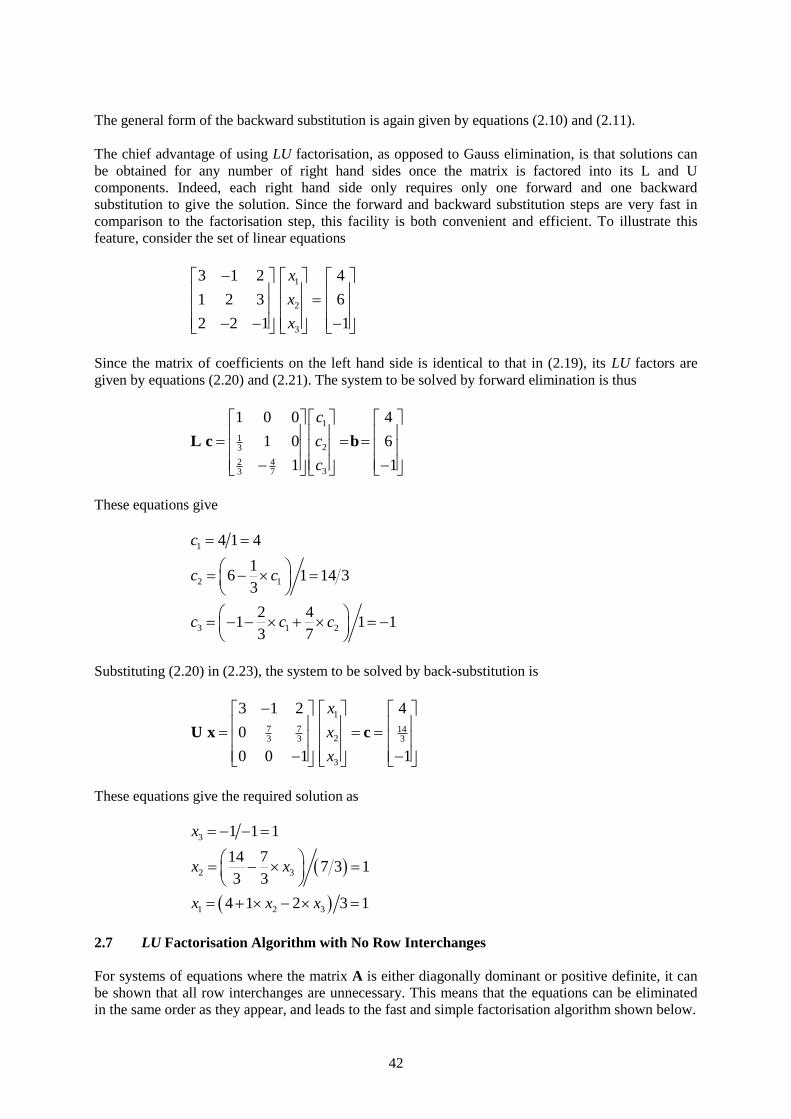
The general form of the backward substitution is again given by equations (2.10) and (2.11).

The chief advantage of using LU factorisation, as opposed to Gauss elimination, is that solutions can

be obtained for any number of right hand sides once the matrix is factored into its L and U

components. Indeed, each right hand side only requires only one forward and one backward

substitution to give the solution. Since the forward and backward substitution steps are very fast in

comparison to the factorisation step, this facility is both convenient and efficient. To illustrate this

feature, consider the set of linear equations

1

2

3

3 1 2 4

1 2 3 6

2 2 1 1

x

x

x

Since the matrix of coefficients on the left hand side is identical to that in (2.19), its LU factors are

given by equations (2.20) and (2.21). The system to be solved by forward elimination is thus

1

123

2 433 7

1 0 0 4

1 0 6

1 1

c

c

c

L c b


1

2 1

3 1 2

4 1 4

16 1 14 3

3

2 41 1 1

3 7

c

c c

c c c

Substituting (2.20) in (2.23), the system to be solved by back-substitution is

1

7 7 1423 3 3

3

3 1 2 4

0

0 0 1 1

x

x

x

U x c

These equations give the required solution as

3

2 3

1 2 3

1 1 1

14 77 3 1

3 3

4 1 2 3 1

x

x x

x x x

2.7 LU Factorisation Algorithm with No Row Interchanges

For systems of equations where the matrix A is either diagonally dominant or positive definite, it can

be shown that all row interchanges are unnecessary. This means that the equations can be eliminated

in the same order as they appear, and leads to the fast and simple factorisation algorithm shown below.

43

LU Factorisation Algorithm with No Row Interchanges

In: Number of equations n, matrix A, pivot tolerance Out: L and U factors or error message.

Original matrix A over-written by L and U factors

comment: L matrix has unit diagonal entries, but these are not stored.

comment: loop over each column k

loop k = 1 to n – 1

comment: perform elimination on rows and cols k+1 to n

loop i = k + 1 to n

comment: check for zero pivot

if ,a k k then

error. equations not diagonally dominant or +ve definite

endif

comment: compute row multiplier and store it in L

m = a i,k a k,k

a i,k = m

loop j = k + 1 to n

a i, j = a i, j - m×a k, j

end loop

end loop

end loop

if thena n,n

error: equations not diagonally dominant or +ve definite

endif

Algorithm 2.1: LU factorisation with no row interchanges

In the above algorithm, the tolerance is used to detect very small pivots. Assuming single precision

arithmetic on a 32 bit computer, with all the entries in A of the order of unity, a suitable value for is

about 610. Note that it is necessary to check for small absolute values, rather than zeros, because of

the effects of roundoff error. Small pivots will not occur if the matrix A is diagonally dominant or

positive definite.

Because the forward and backward substitution phases may be invoked many times for a single

factorisation, it is usual to place these steps in a separate procedure. The forward and backward

substitution steps for Algorithm 2.1 are shown below

Forward and Backward Substitution for LU Factorisation with No Row Interchanges

In: Number of equations n, matrix A, right hand side b.

Out: Solution x.


comment: forward substitution to solve Lc = b

1 = 1x b

44

loop i = 2 to n

sum = 0.

loop j = 1 to i -1

sum = sum + a i, j × x j

end loop

x i = b i - sum

end loop

comment: back-substitution to solve Ux = c

x n = x n a n,n

loop i = n - 1 downto 1

sum = 0.

loop j = i + 1 to n


end loop

x i = x i - sum a i,i

end loop

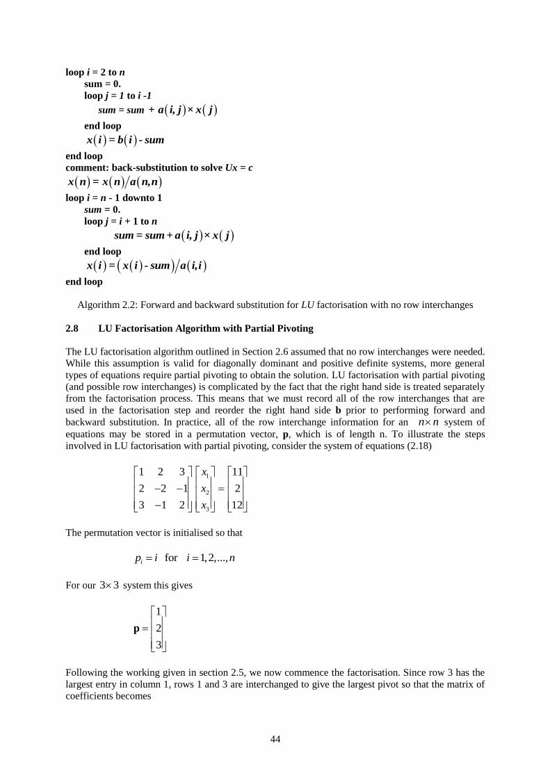
Algorithm 2.2: Forward and backward substitution for LU factorisation with no row interchanges

2.8 LU Factorisation Algorithm with Partial Pivoting

The LU factorisation algorithm outlined in Section 2.6 assumed that no row interchanges were needed.

While this assumption is valid for diagonally dominant and positive definite systems, more general

types of equations require partial pivoting to obtain the solution. LU factorisation with partial pivoting

(and possible row interchanges) is complicated by the fact that the right hand side is treated separately

from the factorisation process. This means that we must record all of the row interchanges that are

used in the factorisation step and reorder the right hand side b prior to performing forward and

backward substitution. In practice, all of the row interchange information for an n n system of

equations may be stored in a permutation vector, p, which is of length n. To illustrate the steps

involved in LU factorisation with partial pivoting, consider the system of equations (2.18)

1

2

3

1 2 3 11

2 2 1 2

3 1 2 12

x

x

x

The permutation vector is initialised so that

for 1,2,...,ip i i n

For our 3 3 system this gives

1

2

3

p

Following the working given in section 2.5, we now commence the factorisation. Since row 3 has the

largest entry in column 1, rows 1 and 3 are interchanged to give the largest pivot so that the matrix of

coefficients becomes

45

3 1 2

2 2 1

1 2 3

(2.25)

Now, to keep track of this interchange, rows 1 and 3 are also swapped in the permutation vector p to

give

3

2

1

p

Applying the elimination steps to (2.25), rows 2 and 3 become

2

2

2

3

22 2 1 3 1 2

3

0 4 3 7 3

11 2 3 3 1 2

3

0 7 3 7 3

j

j

a

a

The multipliers for column 1 of rows 2 and 3 are thus equal to 2/3 and 1/3 respectively, so that

21 312 3 and 1 3l l . Thus, after the first elimination step, we have

72 43 3 3

7 713 3 3

3 1 2

where the factors for L are located in their correct locations in column 1 below the diagonal. Scanning

column 2, from the diagonal down, we see that row 3 has the largest entry for a potential pivot. Prior

to doing the second elimination step, we interchange rows 2 and 3 to give

7 713 3 3

72 43 3 3

3 1 2

(2.26)

Similarly, rows 2 and 3 of the permutation vector p are swapped to give

3

1

2

p (2.27)

After applying the elimination steps to column 2 of (2.26), we obtain the new row 3 as

46

3

3

40 4 3 7 3 0 7 3 7 3

7

0 0 1

ja

The multiplier for column 2 of row 3 is thus equal to –4/7, so that 32 4 7.l This entry is stored in

the second column below the diagonal and we obtain the LU factorisation

7 713 3 3

2 43 7

3 1 2

1

(2.28)

The above equation is stored in compact form. Noting that the lower triangular matrix L has unit

entries on its diagonal, (2.28) may be expanded as

7 713 3 3

2 43 7

1 0 0 3 1 2

1 0 0

1 0 0 1

L U

The permutation vector associated with the factorisation, which contains a complete record of the row

interchanges that were made, is given by (2.27). Before solving the equations, we must first use the

same sequence of interchanges on the right hand side vector b. The entries held in p indicate that the

permuted b vector is given by

3

1

2

12

11

2

b

b

b

b

The system to be solved by forward elimination is thus

13

2 43 7

1 0 0 12

1 0 11

1 2

L c b


1

2 1

3 1 2

12 1 12

111 1 7

3

2 42 1 2

3 7

c

c c

c c c

The system to be solved by back-substitution is then

47

7 73 3

3 1 2 12

0 7

0 0 1 2

U x c

Which gives

3

2 3

1 2 3

2 1 2

77 7 3 1

3

12 1 2 3 3

x

x x

x x x

The steps in performing LU factorisation with partial pivoting may be summarised as follows:

LU Factorisation Algorithm with Partial Pivoting

In: Number of equations n, matrix A, pivot tolerance Out: L and U factors and permutation vector p or error message.



comment: initialise permutation vector p

loop i = 1 to n

p i = i

end loop


loop k = 1 to n –1

comment: find pivot row ip

comment: search column k for entry with max magniture

ip = k

pivot = a k,k

loop i = k+1 to n

thenif a i,k > pivot

ip = i

pivot = a i,k

endif

end loop

comment: check for singular matrix

if pivot ε then

error: equations have no unique solution

endif

48

if ip k then

comment: swap row k with row ip if ip k

loop j = 1 to n

t = a k, j

a k, j = a ip, j

a ip, j = t

end loop

comment: record row swap in permutation vector

comment: swap p(k) with p(ip) if ip k

i = p k

p k = p ip

p ip i

endif

comment: perform elimination on rows and cols k + 1 to n

loop i = k + 1 to n

comment: compute row multiplier and store it in L

m = a i,k a k,k

a i,k = m

loop j = k + 1 to n

a i, j = a i, j - m×a k, j

end loop

end loop

end loop

if a n,n ε

error: equations have no unique solution

endif

Algorithm 2.3: LU factorisation with partial pivoting

In addition to finding the LU factors, which are stored in compact form, the above algorithm also

computes the permutation vector p. The latter is used to permute the right hand side vector b in the

solution phase as shown below.

Forward and Backward Substitution for LU Factorisation with Partial Pivoting

In: Number of equations n, matrix A, right hand side b,

permutation vector p holding row interchanges

Out: Solution x.



x 1 = b p 1

loop i = 2 to n

sum = 0.

loop j = 1 to i – 1


49

end loop

x i = b p i - sum

end loop


x n = x n a n,n

loop i = n – 1 downto 1

sum = 0.

loop j = i +1 to n


end loop

x i = x i - sum a i,i

end loop

Algorithm 2.4: Forward and backward substitution for LU factorisation with partial pivoting

2.9 LU Factorisation Algorithm for Tridiagonal Systems

Tridiagonal matrices are banded so that all their nonzero coefficients lie on the superdiagonal, the

diagonal, and the subdiagonal. More formally a tridiagonal matrix has 0ija whenever 1i j as

shown in the system below

1 1 1 1

2 2 2 2 2

3 3 3 3 3

1 1 1

0 0 0

0 0

0 0

0 0 0 0 0

n n n

n n n n

d u x b

l d u x b

l d u x b

l d u

l d x b

(2.29)

This type of matrix structure occurs frequently in the solution of partial differential equations. In cases

where pivoting is unnecessary, tridiagonal systems can be solved very efficiently using a special form

of LU factorisation. Let us write the LU factorisation of the above matrix as

1 1

2 2 2

3

1 1

1 0 0 0 0 0 0

1 0 0 0 0 0

0 1

0 1 0 0

n n

n n

u

u

LU

u

To determine the unknown coefficients and ,i i we multiply each row of L by the various columns

of U and equate the results to the corresponding elements of the original matrix in (2.29). This gives

1 1d

and

1i i il (2.30)

50

1i i i iu d (2.31)

for i = 2,3,…,n. Equations (2.30) and (2.31) are easily solved to give the entries in and ,i i

according to

1

1

for 2,3,...,

for 2,3,...,

i i i

i i i i

l i n

d u i n

with

1 1d

This completes the LU factorisation. To solve the equations for a given right hand side vector b, we

first perform forward substitution on the equations

1 1

2 2 2

3

1 0 0 0

1 0 0

0 1

0 1n n n

c b

c b

c b

L c b

This gives

1 1

1 for 2,3,...,i i i i

c b

c b c i n

In the backward substitution phase, we need to solve the equations

1 1 1 1

2 2 2 2

1 1

0 0 0

0 0 0

0 0

n n

n n n

u x c

u x c

u

x c

U x c

This gives the solution as

1 for , 1,...,1

n n n

i i i i i

x c

x c u x i n n

The procedure outlined above assumes that no pivoting, with row interchanges, is necessary to obtain

a solution. This can be shown to be true if the following conditions are satisfied

51

1 1

for 1,2,...,i i i

n n

d u

d l u i n

d l

Pivoting is always unnecessary for diagonally dominant or positive definite matrices. Fortunately,

many tridiagonal systems belong to this class.

The steps in performing the above LU factorisation for tridiagonal system of equations may be

summarised as follows

LU Factorisation Algorithm for Tridiagonal Equations

In: Number of equations n, matrix A, pivot tolerance

Subdiagonal of A held in L

Diagonal of A held in D

Superdiagonal held in U

Out: L and U factors or error message.




loop i = 2 to n

comment: check for zero pivot

if d i - 1 then


endif

l i = l i d i - 1

d i = d i - l i × u i - 1

end loop

if d i - 1 then


endif

Algorithm 2.5: LU Factorisation for tridiagonal equations

The forward and backward substitution steps also assume a simple form and are given by

Forward and Backward Substitution for Tridiagonal Equations

In: Number of equations n, factorised matrix A, right hand side b.

Subdiagonal of A held in L

Diagonal of A held in D

Superdiagonal held in U

Out: Solution x.



1 1x = b

loop i = 2 to n

52

x i = b i - l i × x i - 1

end loop


x n = x n d n

loop i = n –1 downto 1

1x i = x i - u i × x i + d i

end loop

Algorithm 2.6: Forward and backward substitution for tridiagonal equations

2.10 Vector and Matrix Norms

In many cases it is useful to be able to measure the ‘size’ of a vector or a matrix. This can be done by

defining a quantity known as a norm. There are three common norms for an arbitrary vector x of

length n.

The sum of magnitudes norm (also known as the 1-norm)

1

1

n

i

i

x

x

The Euclidean norm (also known as the 2-norm)

1/ 2

T 2

21

n

i

j

x

x x x

The maximum norm

1

max ii n

x

x

These norms have three key properties that are normally associated the concept of ‘size’. These

properties are

1. For any vector , 0 0and x x x if and only if x = 0. This condition forces all vectors,

except the zero vector, to have a positive ‘size’.

2. For any vector x and any number a , a ax x . This restriction ensures that a vector x, and

its negative –x, both have the same size. It also stipulates, for example, that the size of the vector

2x is twice the size of the vector x.

3. For any two vectors x and y, x + y x y . This condition is known as the triangle

inequality, since it states that the sum of the lengths of two sides of a triangle is never less than

the length of the third side.

Except in special cases, the various norms will give different values for the size of a vector. To

illustrate the use of the above norms, consider the vectors

T

T

1 10 5

2 15 5

x

y

53

Then

1

2

1 10 5 16

1 100 25 126 11.22

max 1 , 10 , 5 10

x

x

x

and

1

2 2 2

2

1 2 10 15 5 5 28

1 2 10 15 5 5 25.12

max 1 2 , 10 15 , 5 5 25

x + y

x + y

x + y

The ‘closeness’ of two vectors can be measured using the norm of their differences for each

component. For the vectors x and y, we have

1

2 2 2

2

1 2 10 15 5 5 16

1 2 10 15 5 5 11.22

max 1 2 , 10 15 , 5 5 10

x - y

x - y

x - y

Norm of differences are often used to measure errors; for example, x may correspond to a set of true

values and y may correspond to a set of approximate values. It is also possible to compute relative

differences such as

1

1

2

2

161

16

1261

126

101

10

x y

x

x y

x

x y

x

These are particularly useful since they are dimensionless.

A variety of norms may also be defined to describe the ‘size’ of an n n matrix A. Some of the most

widely used, and simplest to compute, are shown below.

The maximum column sum norm (also known as the 1-norm)

1

1

maxn

ijj n i n

a

A

The Euclidean norm (also known as the Frobenius norm)

54

1/ 2

2

1 1

n n

ijei j

a

A

The maximum row sum norm

1

maxn

iji n j n

a

A

Note that the 2-norm (or spectral norm) is difficult to compute since it is related to the eigenvalues of

the matrix. The above matrix norms have the following four key properties

1. For any matrix , 0 0and A A A if and only if A = 0.

2. For any matrix A and any number a a aA A .

3. For any two n n matrices and , A B A B A B .

4. For any two n n matrices and , A B AB A B .

To illustrate the use of matrix norms, consider the matrix

1 2

3 4A

Then

1max 1 3 , 2 4 6

1 4 9 16 30 5.48

max 1 2 , 3 4 7

e

A

A

A

Except in the case of diagonal matrices, the norms do not give the same value for the magnitude of a

matrix.

2.11 Errors and Ill-Conditioning

In solving systems of linear equatins of the form

A x b (2.32)

we are interested in the error in our computed solution x̂ . Note that x̂ , found using some numerical

algorithm, will usually contain rounding errors and is not equal to the exact solution x. The error in our

approximate solution is the difference

ˆ e x x

but, as we do not know the exact solution, this measure is of little practical use. The accuracy of our

computed solution however, can be checked indirectly by calculating the residual

ˆ r b Ax

55

This vector measures how well an approximate solution satisfies the linear equation (2.32). Norms are

useful in measuring the size of r, either as an absolute quantity

absolute residual error r

or as a relative quantity

relative residual error r b (2.33)

The later can, of course, only be used when .b 0 For single precision arithmetic on a computer with

a 32-bit word length, a relative error of about 610 or less would usually signify that an accurate

solution had been obtained. Unfortunately, this is not always the case. To illustrate this point, consider

the pair of equations

1

2

1.01 0.99 2

0.99 1.01 2

x

x

(2.34)

which has the exact solution

1

1

x

with . e r 0 Now, the approximate solution

2

ˆ0

x

has an error of

1

1

e

and a residual of

0.02

0.02

r

As shown below, equation (2.33) gives a relative residual error of only 1 percent, but the relative error

in the solution is 100 percent.

relative residual error 0.02 2 0.01

r b (2.35)

relative solution error 1 1 1

e x (2.36)

Thus, for this case, the size of the residual is a very poor indicator of the accuracy of the solution as it

unduly optimistic. To confuse matters further, the opposite effect can also occur. Consider, for

example, the linear system

56

1

2

1.01 0.99 2

0.99 1.01 2

x

x

(2.37)

which has the exact solution

100

100

x

Now, the approximate solution

101

ˆ99

x

has an error of

1

1

e

and a residual of

2

2

r

For this approximation the relative residual error is 100 percent, but the relative error in the solution is

only 1 percent.

relative residual error 2 2 1

r b (2.38)

relative solution error 1 100 0.01

e x (2.39)

Thus, the relative residual error is again a poor estimate of the accuracy of the solution, but in this case

it is unduly pessimistic.

The puzzling behaviour observed above can be explained in terms of the condition number. The

condition number of a matrix is defined as

1cond A A A (2.40)

and is a direct measure of the ‘sensitivity’ of the equations. Linear equations with large condition

numbers are said to be ill-conditioned. Ill-conditioned equations are characterised by large changes in

the solution for small changes to the right hand side b, a feature which was observed in the previous

example. The precise magnitude of the condition number computed from (2.40) depends on the matrix

norm used and, for some matrices, can vary substantially as the matrix norm is changed.

The condition number permits sharp bounds on the error to be computed using the inequalities

57

1

condcond x

r e r

AA b b

(2.41)

A proof of this relation can be found in most numerical analysis texts and will not be repeated here.

This fundamental inequality is important because it tells us that the relative residual error is only a safe

estimate of the solution accuracy if cond 1.A For cases where the condition number is large, so

that cond 1,A the relative residual does not provide a reliable estimate of the solution error.

Since the exact solution is unknown, it is usual to replace ˆbyx x in (2.41) when typical error bounds

are computed.

To illustrate the effects of a large condition number, let us return to the matrix equations (2.34). For

this case

1

1.01 0.99 25.25 24.75

0.99 1.01 24.75 25.25

A A

so that

max 1.01 0.99 , 0.99 1.01 2 A

and

1 max 25.25 24.75 , 24.75 25.25 50

A

Using (2.40) gives the condition number as

1cond 2 50 100 A A A (2.42)

This value is fairly large, and (2.41) implies that the relative error in the solution can be anywhere

between 100 and 0.01 times the relative residual error. We thus expect the relative residual to provide

an unreliable estimate of the solution error for this system. More specifically, if we have the

approximate solution

2

ˆ0

x

the relative residual error for equations (2.34) is given by (2.35)

0.01

r

b (2.43)

Substituting (2.42) and (2.43) gives the bounds on the relative solution error as

0.0001 1 e

x

The actual relative solution error, from equation (2.36) is

58

1

e

x

and thus corresponds exactly with the theoretical upper bound.

Let us now consider the behaviour of the system (2.37) with the approximate solution vector

101

ˆ99

x

The relative residual error for the equations in this case is given by (2.38) as

1

r

b (2.44)

Substituting (2.42) and (2.44) in (2.41) gives the bounds on the relative solution error according to

0.01 100 e

x

The actual relative solution error, from equation (2.39), is

0.02

e

x

which is very close to the theoretical lower bound.

One disadvantage of using the condition number is that it requires a knowledge of 1.

A Since this

inverse is expensive to compute, many approximate methods for estimating the condition number have

been developed. These procedures, however, are beyond the scope of this course.

2 Direction Solution of Linear Equations

Documents

Transcript of 2 Direction Solution of Linear Equations