5.3 - Consider the system of linear equations: 3x – 2y = 7 5x
Upload
khangminh22Category
view
0download
0
M208 Pure Mathematics
LA2
Linear equations and matrices

Note to reader
Mathematical/statistical content at the Open University is usuallyprovided to students in printed books, with PDFs of the same online.This format ensures that mathematical notation is presentedaccurately and clearly. The PDF of this extract thus shows thecontent exactly as it would be seen by an Open University student.Please note that the PDF may contain references to other parts of themodule and/or to software or audio-visual components of the module.Regrettably mathematical and statistical content in PDF files isunlikely to be accessible using a screenreader, and some OpenLearnunits may have PDF files that are not searchable. You may needadditional help to read these documents.
The Open University, Walton Hall, Milton Keynes, MK7 6AA.
First published 2006.
Copyright c© 2006 The Open University
All rights reserved. No part of this publication may be reproduced, storedin a retrieval system, transmitted or utilised in any form or by any means,electronic, mechanical, photocopying, recording or otherwise, withoutwritten permission from the publisher or a licence from the CopyrightLicensing Agency Ltd. Details of such licences (for reprographicreproduction) may be obtained from the Copyright Licensing Agency Ltd,Saffron House, 6–10 Kirby Street, London EC1N 8TS (websitewww.cla.co.uk).
Open University course materials may also be made available in electronicformats for use by students of the University. All rights, includingcopyright and related rights and database rights, in electronic coursematerials and their contents are owned by or licensed to The OpenUniversity, or otherwise used by The Open University as permitted byapplicable law.
In using electronic course materials and their contents you agree that youruse will be solely for the purposes of following an Open University courseof study or otherwise as licensed by The Open University or its assigns.
Except as permitted above you undertake not to copy store in any medium(including electronic storage or use in a website), distribute, transmit orretransmit, broadcast, modify or show in public such electronic materials inwhole or in part without the prior written consent of The Open Universityor in accordance with the Copyright, Designs and Patents Act 1988.
ISBN 0 7492 0223 8
1.1
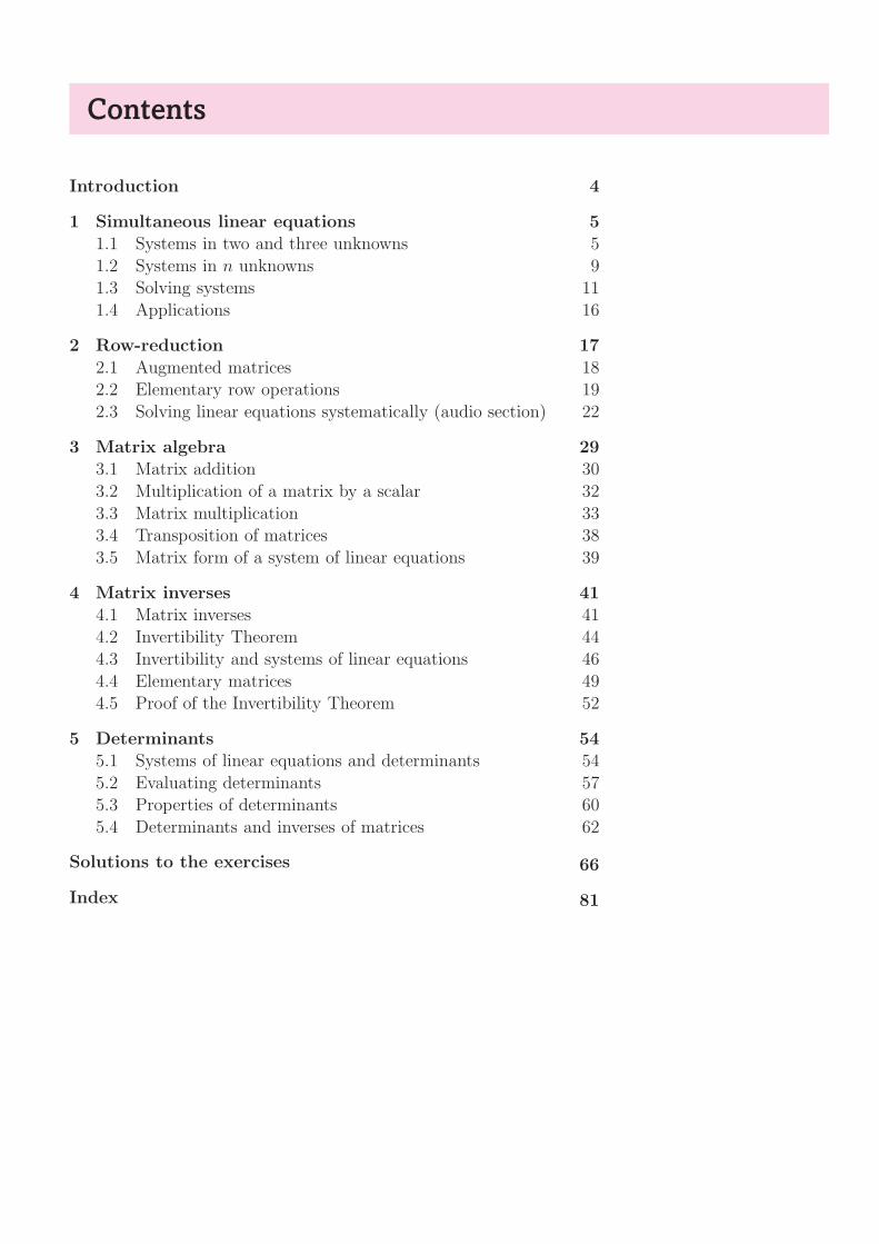
Contents
Introduction 4
1 Simultaneous linear equations 51.1 Systems in two and three unknowns 5
1.2 Systems in n unknowns 91.3 Solving systems 11
1.4 Applications 16
2 Row-reduction 17
2.1 Augmented matrices 182.2 Elementary row operations 19
2.3 Solving linear equations systematically (audio section) 22
3 Matrix algebra 293.1 Matrix addition 30
3.2 Multiplication of a matrix by a scalar 32
3.3 Matrix multiplication 333.4 Transposition of matrices 38
3.5 Matrix form of a system of linear equations 39
4 Matrix inverses 414.1 Matrix inverses 41
4.2 Invertibility Theorem 444.3 Invertibility and systems of linear equations 46
4.4 Elementary matrices 494.5 Proof of the Invertibility Theorem 52
5 Determinants 545.1 Systems of linear equations and determinants 54
5.2 Evaluating determinants 575.3 Properties of determinants 60
5.4 Determinants and inverses of matrices 62
66Solutions to the exercises
Index 81

Unit LA2 Linear equations and matrices
Introduction
Systems of simultaneous linear equations arise frequently in mathematicsand in many other areas. For example, in Unit LA1 you found the point ofintersection of a pair of non-parallel lines in R
2 by solving the twoequations of the lines as simultaneous equations—that is, by finding thevalues for x and y that simultaneously satisfy both equations. In particular,you found the solution to the system of simultaneous linear equations
{
3x − y = 1,x − y = −1,
to be x = 1, y = 2. In other words, the two lines 3x− y = 1 andx− y = −1 intersect at the point (1, 2).
The solution to a system of simultaneous linear equations in two unknowns(x and y) corresponds to the points of intersection (if any) of lines in R
2.Similarly, solutions to systems of linear equations in three unknowns Recall from Unit LA1,
Subsection 1.2, that an equationof the form 2x+ 3y + 4z = 5represents a plane in R
3.
correspond to the intersection (if any) of planes in R3. Although systems
with more unknowns can be thought of in relation to intersections inspaces of higher dimension, we develop a strategy for solving such systemswithout the need to visualise a multi-dimensional world!
Matrices appear throughout mathematics. In this unit we assume no priorknowledge of matrices, although you may well have met them before. Weuse matrices as a concise way of representing systems of linear equations,and then go on to study matrix algebra and determinants. Throughoutthis unit we relate our results to the solutions of systems of simultaneouslinear equations. Many of the ideas and methods introduced here will beused in the following three units on linear algebra.
In Section 1 we begin by considering simultaneous linear equations in twoand three unknowns. We introduce the idea of a solution set, and interpretour results geometrically. We then generalise these ideas to systems ofm simultaneous linear equations in n unknowns, and introduce the methodof Gauss–Jordan elimination to solve them systematically.
In Section 2 we develop a strategy for solving systems of linear equations,based on performing elementary row operations on the augmented matrix
of the system in question. We transform the augmented matrix torow-reduced form, from which we can easily read off any solutions. Thismethod is algorithmic, and a computer can be programmed to perform it; Most computer programs use a
slightly modified version of thismethod.
this enables large systems with many unknowns to be handled efficiently.
In Section 3 we study the algebra of matrices. We investigate the additionand scalar multiplication of matrices, and see that matrices can be thoughtof as a generalisation of vectors. We use the dot product of vectors todefine the multiplication of one matrix by another. Finally, we introducesome important types of matrices, and the matrix operation oftransposition—interchanging the rows and columns of a matrix—whichwill be used later in the block.
In Section 4 we introduce the inverse of a matrix. This plays a role inmatrix arithmetic similar to that of the reciprocal of a number in ordinaryarithmetic. We show that many matrices do not have inverses, and give amethod for finding an inverse when it does exist. We also link the idea ofthe invertibility of a matrix with the number of solutions of some systemsof linear equations.
4

Section 1 Simultaneous linear equations
In Section 5 we use systems of linear equations to introduce thedeterminant of a square matrix. The determinant assigns to each squarematrix a number which characterises certain properties of the matrix. Inparticular, we prove that a matrix is invertible if and only if itsdeterminant is non-zero; this provides a method for determining whetheror not a given matrix is invertible.
Study guideSections 1 to 5 should be studied in the natural order.
Section 1 is straightforward and should not take you long.
Section 2 is the audio section. Using row-reduction to solve systems oflinear equations is an important method to master.
Much of Section 3 may be revision for you. If you have not multipliedmatrices before, then you will need to spend some time practising this as itmay seem strange at first. Matrix multiplication plays an important partin the remainder of the block.
Sections 4 and 5 both contain important material. There is a lot of theoryin these sections, and you need not master it completely. You should,however, make sure that you can find the inverse and evaluate thedeterminant of a 2× 2 or 3× 3 matrix, and you should at least read thestatements of the theorems.
1 Simultaneous linear equations
After working through this section, you should be able to:
(a) understand the connection between the solutions of systems ofsimultaneous linear equations in two and three unknowns and theintersection of lines and planes in R
2 and R3;
(b) describe the three types of elementary operation;
(c) use the method of Gauss–Jordan elimination to find the solutionsof systems of simultaneous linear equations;
(d) explain the terms solution set, consistent, inconsistent andhomogeneous system of simultaneous linear equations.
1.1 Systems in two and three unknowns
Systems in two unknowns
One equation
Recall that an equation of the form Unit LA1, Subsection 1.1.
ax+ by = c Here, a, b and c are realnumbers, and a and b are notboth zero.represents a line in R
2. There are infinitely many solutions to thisequation—one corresponding to each point on the line.
5

Unit LA2 Linear equations and matrices
Two equations
The solutions to the system of two simultaneous linear equations{
ax + by = c,dx + ey = f,
Here, a, b, . . . , f are realnumbers.
in the two unknowns x and y correspond to the points of intersection ofthese two lines in R
2.
Two arbitrary lines in R2 may intersect at a unique point, be parallel or Unit LA1, Subsection 1.1.
coincide. This means that solving a system of two simultaneous linearequations in two unknowns yields exactly one of the following threesituations.
• There is a unique solution, when the two lines that the equationsrepresent intersect at a unique point.
For example, the system{
x − y = −1,2x + y = 4,
has the unique solution x = 1, y = 2, corresponding to the uniquepoint of intersection (1, 2) of the two lines in R
2.
• There is no solution, when the two lines that the equations representare parallel.
For example, the system{
x − y = −1,x − y = 1,
represents two parallel lines in R2, which do not intersect, and so has
no solutions.
• There are infinitely many solutions, when the two lines that theequations represent coincide.
For example, the system{
−6x + 3y = −6,2x − y = 2,
has infinitely many solutions, as the two equations represent the sameline in R
2. In a sense, the two lines intersect at each of their points;that is, each pair of values for x and y satisfying 2x− y = 2 is asolution to this system.
Systems in three unknowns
One equation
Recall that an equation of the form Unit LA1, Subsection 1.2.
ax+ by + cz = d Here, a, b, c and d are realnumbers, and a, b and c are notall zero.represents a plane in R
3. There are infinitely many solutions to thisequation—one corresponding to each point in the plane.
6

Section 1 Simultaneous linear equations
Two equations
The solutions to the system of two simultaneous linear equations{
ax + by + cz = d,ex + fy + gz = h,
Here, a, b, . . . , h are realnumbers.
in the three unknowns x, y and z correspond to the points of intersectionof these two planes in R
3.
Two arbitrary planes in R3 may intersect, be parallel or coincide. In Unit LA1, Subsection 1.2.
general, when two distinct planes in R3 intersect, the set of common points
is a line that lies in both planes. This means that solving a system of twosimultaneous linear equations in three unknowns yields exactly one of thefollowing two situations.
• There is no solution, when the two planes that the equations representare parallel.
For example, the system{
x + y + z = 1,x + y + z = 2,
represents two parallel planes in R3 and so has no solutions.
• There are infinitely many solutions, when the two planes that theequations represent coincide, or when they intersect in a line.
For example, the system{
x + y + z = 1,2x + 2y + 2z = 2,
has infinitely many solutions, as the two equations represent the sameplane in R
3. Each set of values for x, y and z satisfying x+ y + z = 1is a solution to this system, such as x = 1, y = 0, z = 0 and x = −2,y = 4, z = −1.
Similarly, the system{
x + y + z = 1,x + y = 1,
has infinitely many solutions: the planes in R3 represented by the two
equations intersect in a line. The z-coordinate of each point on thisline is zero, so the line lies in the (x, y)-plane. Each set of values for x,y and z satisfying x+ y = 1 and z = 0 is a solution to this system,such as x = 1, y = 0, z = 0 and x = 5, y = −4, z = 0.
Three equations
In a similar way, the solutions to the system of three simultaneous linearequations
ax + by + cz = d,ex + fy + gz = h,ix + jy + kz = l,
Here, a, b, . . . , l are real numbers.
in the three unknowns x, y and z correspond to the points of intersectionof these three planes in R
3.
Three arbitrary planes in R3 may meet each other in a number of different
ways. We illustrate these possibilities below.
7
Unit LA2 Linear equations and matrices
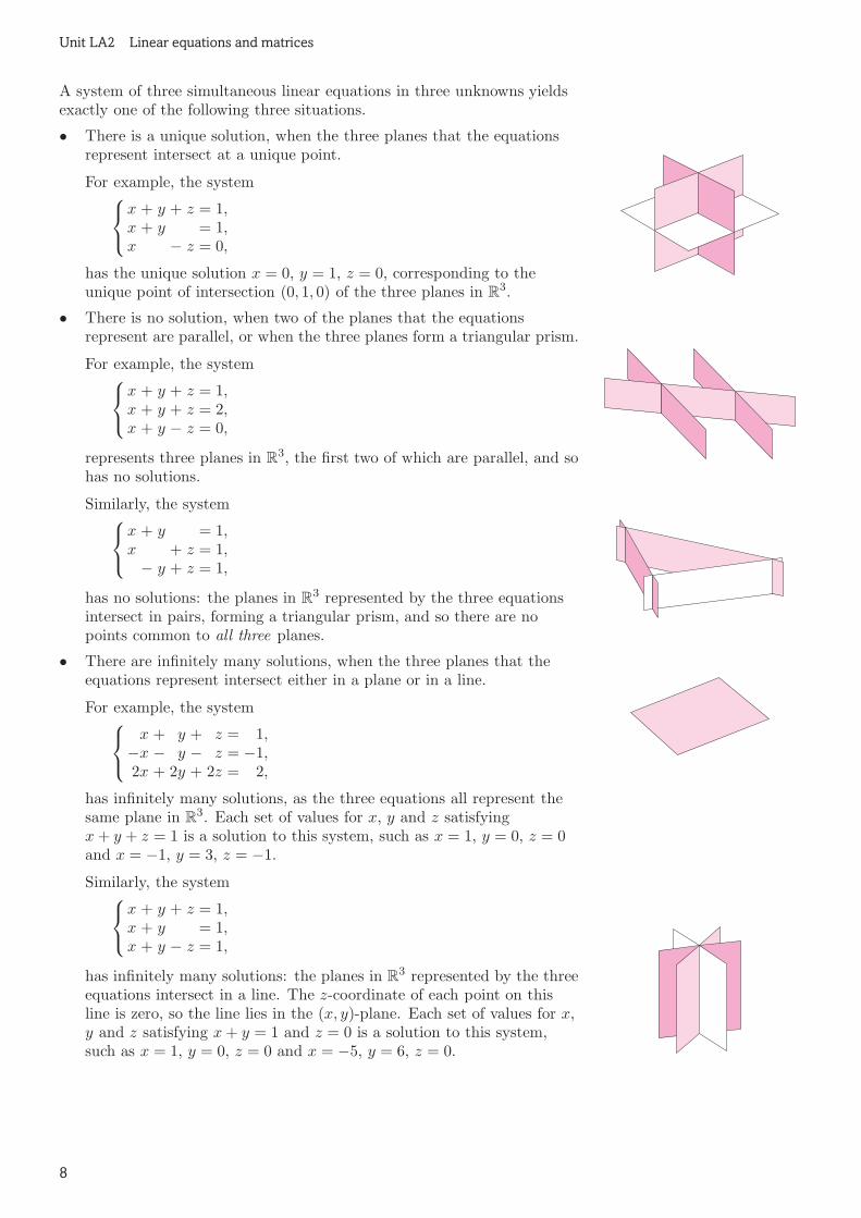
A system of three simultaneous linear equations in three unknowns yieldsexactly one of the following three situations.
• There is a unique solution, when the three planes that the equationsrepresent intersect at a unique point.
For example, the system
x + y + z = 1,x + y = 1,x − z = 0,
has the unique solution x = 0, y = 1, z = 0, corresponding to theunique point of intersection (0, 1, 0) of the three planes in R
3.
• There is no solution, when two of the planes that the equationsrepresent are parallel, or when the three planes form a triangular prism.
For example, the system
x + y + z = 1,x + y + z = 2,x + y − z = 0,
represents three planes in R3, the first two of which are parallel, and so
has no solutions.
Similarly, the system
x + y = 1,x + z = 1,− y + z = 1,
has no solutions: the planes in R3 represented by the three equations
intersect in pairs, forming a triangular prism, and so there are nopoints common to all three planes.
• There are infinitely many solutions, when the three planes that theequations represent intersect either in a plane or in a line.
For example, the system
x + y + z = 1,−x − y − z = −1,2x + 2y + 2z = 2,
has infinitely many solutions, as the three equations all represent thesame plane in R
3. Each set of values for x, y and z satisfyingx+ y + z = 1 is a solution to this system, such as x = 1, y = 0, z = 0and x = −1, y = 3, z = −1.
Similarly, the system
x + y + z = 1,x + y = 1,x + y − z = 1,
has infinitely many solutions: the planes in R3 represented by the three
equations intersect in a line. The z-coordinate of each point on thisline is zero, so the line lies in the (x, y)-plane. Each set of values for x,y and z satisfying x+ y = 1 and z = 0 is a solution to this system,such as x = 1, y = 0, z = 0 and x = −5, y = 6, z = 0.
8

Section 1 Simultaneous linear equations
1.2 Systems in n unknownsThe equations for a line in R
2 and a plane in R3 are linear equations in
two and three unknowns, respectively. Similarly, an equation of the formHere, a, . . . , e are real numbers,and a, b, c and d are not all zero.ax+ by + cz + dw = e
is a linear equation in the four unknowns x, y, z and w. In general, we candefine a linear equation in any number of unknowns.
Definitions An equation of the form
a1x1 + a2x2 + · · ·+ anxn = b, A linear equation has no termsthat are products of unknowns,such as x2
1 or x1x4.where a1, a2, . . . , an, b are real numbers, and a1, . . . , an are not allzero, is a linear equation in the n unknowns x1, x2, . . . , xn. Thenumbers ai are the coefficients, and b is the constant term.
Exercise 1.1 Which of the following are linear equations in theunknowns x1, . . . , x5?
(a) x1 + 3x2 − x3 − 5x4 − 2x5 = 0 (b) x1 − x2 + 2x3x4 + 3x5 = 4
(c) 5x2 − x5 = 2 (d) a1x1 + a2x22 + · · · + a5x
55 = b
We write a general system of m simultaneous linear equations in Frequently, we refer simply tosystems of linear equations, asthe full description is rather amouthful!
n unknowns as
a11x1 + a12x2 + · · · + a1nxn = b1,a21x1 + a22x2 + · · · + a2nxn = b2,...
......
...am1x1 + am2x2 + · · · + amnxn = bm.
The numbers bi are the constant terms, the variables xi are the unknownsand the numbers aij are the coefficients. We use the double subscript ij toshow that aij is the coefficient of the jth unknown in the ith equation.The number m of equations need not be the same as the number n ofunknowns.
A solution of a system of linear equations is a list of values for theunknowns that simultaneously satisfy each of the equations. In solving asystem, we look for all the solutions—you have already seen that somesystems have infinitely many solutions.
Definitions The values x1 = c1, x2 = c2, . . . , xn = cn are a solution
of a system of m simultaneous linear equations in n unknowns,x1, . . . , xn, if these values simultaneously satisfy all m equations of thesystem. The solution set of the system is the set of all the solutions.
For example, you saw earlier that the solution set of the system
x + y + z = 1,x + y = 1,x − z = 0,
(1.1)
is the set {(0, 1, 0)}, which has just one member.
9

Unit LA2 Linear equations and matrices
You also saw that the solution set of the system
x + y + z = 1,x + y + z = 2,x + y − z = 0,
(1.2)
is the empty set.
Definitions A system of simultaneous linear equations is consistentwhen it has at least one solution, and inconsistent when it has nosolutions.
The system (1.1) is consistent, and the system (1.2) is inconsistent.
When a system of linear equations has infinitely many solutions, we canwrite down a general solution from which all solutions can be found. Weillustrate this with an example that you have already met.
You saw earlier that the solutions of the system
x + y + z = 1,x + y = 1,x + y − z = 1,
are the sets of values for x, y and z satisfying x+ y = 1 and z = 0. Theunknowns x and y are related by the equation x+ y = 1, which we canrewrite as y = 1− x. Thus for each real parameter k assigned to theunknown x, we have a corresponding value 1− k for the unknown y. Wewrite this general solution as
x = k, y = 1− k, z = 0, where k ∈ R.
To highlight the connection between the solutions of the system and theintersection of the planes in R
3, we can write the solution set as a set ofpoints in R
3: The order of the unknowns mustbe clear—the triples (1, 0, 0) and(0, 1, 0) correspond to differentsolutions.
{(k, 1 − k, 0) : k ∈ R}.
Homogeneous systems
In the following systems of linear equations, the constant terms are all zero:{
2x + 3y = 0,x − y = 0;
(1.3)
x − y − z = 0,2x + y − z = 0,−x + y + z = 0.
(1.4)
Such systems are called homogeneous.
Definitions A homogeneous system of linear equations is a systemof simultaneous linear equations in which each constant term is zero.
A system containing at least one non-zero constant term is anon-homogeneous system.
If we substitute x = 0, y = 0 into system (1.3), and x = 0, y = 0, z = 0into system (1.4), then all the equations are satisfied. These solutions arecalled trivial.
10
Section 1 Simultaneous linear equations
Definitions The trivial solution to a system of simultaneous linearequations is the solution with each unknown equal to zero.
A solution with at least one non-zero unknown is a non-trivial
solution.
A homogeneous system always has at least the trivial solution, and is Non-homogeneous systems haveonly non-trivial solutions.therefore always consistent.
Exercise 1.2 Write down a general homogeneous system of m linearequations in n unknowns, and show that the solution set contains thetrivial solution.
Returning to system (1.4), we see that there are other solutions. For System (1.3) has no non-trivialsolutions.example, x = 2, y = −1, z = 3 is a solution. In fact, this system has an
infinite solution set, which we can write as
{(2k,−k, 3k) : k ∈ R}.
Number of solutions
We have already seen that when m ≤ n ≤ 3, a system of m equations inn unknowns has a solution set which
• contains exactly one solution,
• or is empty,
• or contains infinitely many solutions.
In fact, the solution set of a system of m linear equations in n unknowns This assertion will be proved inUnit LA4.has one of these forms, for any m and n.
We saw earlier that two non-parallel planes in R3 cannot intersect in a
unique point. A consistent system of two linear equations in threeunknowns therefore has an infinite solution set. In general, a consistentsystem of m equations in n unknowns, with m < n, has insufficientconstraints on the unknowns to determine them uniquely; that is, it has aninfinite solution set.
1.3 Solving systemsWe now introduce a systematic method for solving systems of simultaneous You will meet this method again
in Section 2, where you will usematrices to represent systems oflinear equations. A strategy isgiven there.
linear equations. This method is called Gauss–Jordan elimination. Itentails successively transforming a system into simpler systems, in such away that the solution set remains unchanged. The process ends when thesolutions can be determined easily.
The idea is to reduce the number of unknowns in each equation. Ingeneral, we use the first equation to eliminate the first unknown from allthe other equations, then use the second equation to eliminate anotherunknown (usually the second) from all the other equations, and so on.
To avoid confusion when applying this method, we label the currentequations r1, r2, and so on. We can then write down how we are The same notation, r1, r2, and
so on, will be used in Section 2where we transform rows ofmatrices, hence the choice of theletter r.
transforming the preceding system to obtain the current (simpler) system.We use the symbol ↔ (‘interchanges with’) to indicate that two equationsare to be interchanged; for example, r1 ↔ r2 means that the first andsecond equations are interchanged. We use the symbol → (‘goes to’) toshow how an equation is to be transformed. For example, r2 → r2 + r1means that the second equation of the system is transformed by adding thefirst equation to it.
11

Unit LA2 Linear equations and matrices
We start by illustrating this method with a system of two linear equationsin two unknowns. Although this method is not the simplest way of solvingthis particular system, it proves very useful in solving more complicatedsystems.
Example 1.1 Solve the following system of two linear equations in twounknowns:
{
2x + 4y = 10,4x + y = 6.
Solution We aim to simplify the system by eliminating the unknown y In other words, we aim to reducethe system to the form{
x = ∗,y = ∗,
where the asterisks denotenumbers to be determined.
from the first equation and the unknown x from the second. Theoperations we perform do not alter the solution set of the system.
We label the two equations of the system:
r1r2
{
2x + 4y = 10,4x + y = 6.
We begin by simplifying the first equation; we divide it through by 2, sothat the coefficient of x is equal to 1: At each step, we relabel
(implicitly) the equations of thecurrent system. These twoequations therefore become thenew r1 and r2.
r1 →1
2r1
{
x + 2y = 5,4x + y = 6.
We then transform this system into a system with no x-term in the secondequation. To do this, we subtract 4 times the first equation from thesecond:
r2 → r2 − 4r1
{
x + 2y = 5,− 7y = −14.
We now simplify the second equation of this new system by dividingthrough by −7. This yields a system which already looks less complicatedthan the original system, but has the same solution set:
r2 → −1
7r2
{
x + 2y = 5,y = 2.
We next use this new second equation to eliminate the y-term from thefirst equation. We subtract twice the second equation from the first, whichyields the system
r1 → r1 − 2r2{
x = 1,y = 2.
We conclude that there is a unique solution—namely, x = 1, y = 2.
In calculations of this sort, errors are easily made. It is therefore advisableto check the solution by substituting it back into the equations of theoriginal system. For this example, substituting x = 1 and y = 2, we findthat
{
(2× 1) + (4× 2) = 10, X
(4× 1) + (1× 2) = 6. X
The steps we performed in this example involve either multiplying (ordividing) an equation by a non-zero number, or changing one equation byadding (or subtracting) a multiple of another. Neither of these operationsalters the solution set of the system. Changing the order in which we writedown the equations also does not alter the solution set of the system.These are the three operations, called elementary operations, that weperform to simplify a system of linear equations when using the method ofGauss–Jordan elimination.
12

Section 1 Simultaneous linear equations
Elementary operations The following operations do not change thesolution set of a system of linear equations.
1. Interchange two equations.
2. Multiply an equation by a non-zero number.Operation 2 includes division bya non-zero number.
3. Change one equation by adding to it a multiple of another. Operation 3 includes subtractinga multiple of one equation fromanother.
Exercise 1.3 Solve the following system of two linear equations intwo unknowns:
{
x + y = 4,2x − y = 5,
by performing elementary operations to simplify the system as inExample 1.1.
We now solve a system of three linear equations in three unknowns. Weuse elementary operations to try to reduce the system to the form
x = ∗,y = ∗,
z = ∗.Here, the asterisks denotenumbers to be determined.
Example 1.2 Solve the following system of three linear equations inthree unknowns:
x + y + 2z = 3,2x + 2y + 3z = 5,x − y = 5.
Solution We label the three equations of the system:
r1r2r3
x + y + 2z = 3,2x + 2y + 3z = 5,x − y = 5.
We begin the simplification by using the first equation to eliminate thex-term from the second and third equations:
r2 → r2 − 2r1r3 → r3 − r1
x + y + 2z = 3,− z = −1,
− 2y − 2z = 2.
We now have no y-term in the second equation, and so cannot use thisequation to eliminate the y-term from the first and third equations. Wealso cannot use the first equation to eliminate the y-term from the thirdequation, as this would reintroduce an x-term. We therefore interchangethe second and third equations, to obtain a non-zero y-term in the newsecond equation:
r2 ↔ r3
x + y + 2z = 3,− 2y − 2z = 2,
− z = −1.
We simplify this new second equation by dividing through by −2:
r2 → −1
2r2
x + y + 2z = 3,y + z = −1,− z = −1.
13

Unit LA2 Linear equations and matrices
We can now use the second equation to eliminate the y-term from the firstequation:
r1 → r1 − r2
x + z = 4,y + z = −1,− z = −1.
We simplify the third equation by multiplying through by −1:
r3 → −r3
x + z = 4,y + z = −1,
z = 1.
Finally, we use the third equation to eliminate the z-term from the firstand second equations:
r1 → r1 − r3r2 → r2 − r3
x = 3,y = −2,
z = 1.
We conclude that there is a unique solution—namely, x = 3, y = −2, You should check this solutionby substituting it into theoriginal equations.
z = 1.
Exercise 1.4 Solve the following system of three linear equations inthree unknowns:
x + y − z = 8,2x − y + z = 1,−x + 3y + 2z = −8.
Each example solved in this subsection has a unique solution. We nowshow how to apply the method to a system that does not have a uniquesolution.
It is not usually possible to reduce a system with an infinite solution set toone where each equation contains just one unknown. This is illustrated bythe following example.
Example 1.3 Solve the following system of three linear equations inthree unknowns:
x + 2y = 0,y − z = 2,
x + y + z = −2.
Solution We label the three equations, and apply elementary operationsto simplify the system. To save space, we write the explanations to theright of the equations.
r1r2r3
x + 2y = 0y − z = 2
x + y + z = −2We label the equations.
r3 → r3 − r1
x + 2y = 0y − z = 2
− y + z = −2
We eliminate the x-term from r3using r1.
r1 → r1 − 2r2
r3 → r3 + r2
x + 2z = −4y − z = 2
0x + 0y + 0z = 0
We eliminate the y-terms fromr1 and r3 using r2.
14

Section 1 Simultaneous linear equations
We have written the current r3 equation as 0x+ 0y + 0z = 0 to highlightthe fact that all the coefficients are zero, although in future examples weshall simply write 0 = 0. This equation gives no constraints on x, y and z. ‘No constraints’ means that any
values for x, y and z satisfy theequation.If we were to try to use equation r2 to eliminate the z-term from r1, we
would reintroduce a y-term. Similarly, using equation r1 to eliminate thez-term from the equation r2 would reintroduce an x-term.
The system has an infinite solution set, as there are insufficient constraintson the unknowns to determine them uniquely. We have two equations, onerelating the unknowns x and z, and the other relating y and z. As each x = −4− 2z and y = 2 + z.
equation involves a z-term, we can choose any value we wish for z, andwrite the general solution as
x = −4− 2k, y = 2 + k, z = k, k ∈ R.
Whenever the simplification results in an equation 0 = 0, we have, ineffect, reduced the number of equations. We simplify the remainingequations as far as possible, in order to determine the solution set.
Exercise 1.5 Solve the following system of three linear equations inthree unknowns:
x + 3y − z = 4,−x + 2y − 4z = 6,x + 2y = 2.
We now try to solve an inconsistent system.
Example 1.4 Solve the following system of three linear equations inthree unknowns:
x + 2y + 4z = 6,y + z = 1,
x + 3y + 5z = 10.
Solution We apply elementary operations to simplify the system.
r1r2r3
x + 2y + 4z = 6y + z = 1
x + 3y + 5z = 10We label the equations.
r3 → r3 − r1
x + 2y + 4z = 6y + z = 1y + z = 4
We eliminate the x-term from r3using r1.
r1 → r1 − 2r2
r3 → r3 − r2
x + 2z = 4y + z = 1
0 = 3
We eliminate the y-terms fromr1 and r3 using r2.
Concentrating on the current r3 equation (0 = 3), we see that there are no Compare this equation with thefinal equation r3 in the solutionto Example 1.3.
values of x, y and z that satisfy it. The solution set of this system of linearequations is the empty set.
Whenever the simplification results in an equation 0 = ∗, where theasterisk ∗ denotes a non-zero number, we have an inconsistent system, asthis equation has no solutions. There is no point in simplifying theremaining equations further. In fact, in Example 1.4, inconsistency of thesystem could have been inferred at the penultimate stage, as the equationsy + z = 1 and y + z = 4 form an inconsistent system.
15

Unit LA2 Linear equations and matrices
Exercise 1.6 Solve the following system of three linear equations inthree unknowns:
x + y + z = 6,−x + y − 3z = −2,2x + y + 3z = 6.
1.4 ApplicationsSystems of simultaneous linear equations frequently arise when we usemathematics to solve problems; that is, when we formulate a mathematicalmodel to help solve a problem.
In general, to model any straightforward problem we follow the same basicprocedure.
1. Identify the unknowns.
2. Analyse each statement of the problem, and rewrite it as an equationrelating the unknowns.
3. Solve these equations.
4. Write the solution in words to answer the problem, checking that it‘makes sense’.
These four steps are illustrated in the following example.
Example 1.5 The sum of the ages of my sister and my brother is40 years. My brother is 12 years older than my sister. How old is mysister?
Solution First we decide what the unknowns are. Here we are asked to This is step 1.
find the age of my sister, so this is obviously one unknown. The statementrelates my sister’s age to my brother’s age. We do not know my brother’sage, so this is a second unknown. These are the only two unknowns in thisproblem. Let us denote my sister’s age by s and my brother’s age by b (inyears).
The first statement of the problem now translates to the equation This is step 2.
s+ b = 40,
and the second statement to
b = s+ 12.
We write these two equations in the usual form:{
s + b = 40,−s + b = 12.
This system could be solved more simply but, as a further illustration of This is step 3.
the method, we apply elementary operations to simplify it.
r1r2
{
s + b = 40−s + b = 12
We label the equations.
r2 → r2 + r1
{
s + b = 402b = 52
We eliminate the s-term from r2using r1.
r2 →1
2r2
{
s + b = 40b = 26
We simplify r2 by dividingthrough by 2.
16

Section 2 Rowreduction
r1 → r1 − r2{
s = 14b = 26
Finally, we eliminate the b-termfrom r1 using r2.
The system has a unique solution—namely, s = 14, b = 26.
The answer to the problem is that my sister is 14 years old. This makes This is step 4.
sense, as it is positive and not an unreasonable age. (An age of 612 yearswould be unreasonable!) We also note that 14 and 26 do add to 40, andthat 26 is 12 more than 14.
Further exercisesExercise 1.7 Find the solution set of each of the following systems ofsimultaneous linear equations.
(a)
x + 4y = −72x − y = 4−x + 2y = −5
(b)
{
4x − 6y = −2−6x + 9y = −3
(c)
p + q + r = 5p + 2q + 3r = 11
3p + q + 4r = 13
Exercise 1.8 Find the points of intersection of the planes x+ y − z = 0,y − 2z = 0 and 3x− y + 5z = 0 in R
3.
Exercise 1.9 Solve the following system of simultaneous linear equationsin four unknowns.
a − b − 2c + d = 3b + c + d = 3
a − b − c + 2d = 7b + c + 2d = 7
2 Rowreduction
After working through this section, you should be able to:
(a) write down the augmented matrix of a system of linear equations,and recover a system of linear equations from its augmentedmatrix;
(b) describe the three types of elementary row operation;
(c) recognise whether or not a given matrix is in row-reduced form;
(d) row-reduce a matrix;
(e) solve a system of linear equations by row-reducing its augmentedmatrix.
In this section we give a systematic method for solving a system of linearequations by Gauss–Jordan elimination. This method makes it easy tosolve even quite large systems of linear equations. It involves a technique(row-reduction) that will be useful in another context later in this unit.
17

Unit LA2 Linear equations and matrices
2.1 Augmented matricesWe begin by introducing an abbreviated notation for a system of linearequations.
You may have met the notion of a matrix at some point in your study ofmathematics. A matrix is simply a rectangular array of objects, usuallynumbers, enclosed in brackets. Here are some examples:
2 −7−1 1
2
0 12
,
(
3.17 2.23 7.05 0.004.88 1.71 1.72 5.55
)
,
3 7 12−2 17 811 7 −5
.In M208 we use round bracketsfor matrices; some texts usesquare ones.
The objects in a matrix are called its entries. The entries along ahorizontal line form a row, and those down a vertical line form a column.
For example, the first row of the first matrix above is 2 −7, and the second
column of the same matrix is
−71
2
12
.
We can abbreviate a system of linear equations by writing its coefficientsand constants in the form of a matrix. For example, the system
{
4x + y = −7,x − 3y = 0,
can be abbreviated as It is helpful to draw a verticalline separating the coefficients ofthe unknowns on the left-handsides of the equations from theconstants on the right-handsides.
(
4 1 −71 −3 0
)
.
In general, the system
a11x1 + a12x2 + · · · + a1nxn = b1,a21x1 + a22x2 + · · · + a2nxn = b2,...
......
...am1x1 + am2x2 + · · · + amnxn = bm,
of m linear equations in n unknowns x1, x2, . . . , xn is abbreviated as thematrix
a11 a12 · · · a1n b1a21 a22 · · · a2n b2...
......
...am1 am2 · · · amn bm
.
This matrix is called the augmented matrix of the system. The wordaugmented reflects the fact that this is made up of a matrix formed by thecoefficients of the unknowns on the left-hand sides of the equations,augmented by a matrix formed by the constants on the right-hand sides.Later, we shall sometimes consider these two matrices separately.
In the augmented matrix, each row corresponds to an equation, and eachcolumn (except the last) corresponds to an unknown, in the sense that itcontains all the coefficients of that unknown from the various equations.The last column corresponds to the right-hand sides of the equations.
Example 2.1 Write down the augmented matrix of the following system Before writing down theaugmented matrix of a system oflinear equations, we must ensurethat the unknowns appear in thesame order in each equation,with gaps left for ‘missing’unknowns (that is, unknownswhose coefficient is 0).
of linear equations:
x + 0y + 10z = 5,3x + y − 4z = −1,4x − 2y + 6z = 1.
18

Section 2 Rowreduction
Solution The augmented matrix of the system is
1 0 10 53 1 −4 −14 −2 6 1
.
Example 2.2 Write down the system of linear equations correspondingto the following augmented matrix, given that the unknowns are, in order,x1, x2:
1 −2 50 1 94 3 0
.
Solution The corresponding system is
x1 − 2x2 = 5,x2 = 9,
4x1 + 3x2 = 0.
Exercise 2.1
(a) Write down the augmented matrix of the following system oflinear equations:
4x1 − 2x2 = −7,x2 + 3x3 = 0,
− 3x2 + x3 = 3.
(b) Write down the system of linear equations corresponding to thefollowing augmented matrix, given that the unknowns are, inorder, x, y, z, w:
2 3 0 7 10 1 −7 0 −11 0 3 −1 2
.
2.2 Elementary row operationsWhen we used Gauss–Jordan elimination to solve a system of linearequations in Section 1, we worked directly with the system itself; but it isoften easier to apply the same method to its abbreviated form, theaugmented matrix. The three elementary operations on the equations ofthe system correspond exactly to three equivalent operations on the rowsof its augmented matrix.
Recall that the three elementary operations are as follows. Subsection 1.3
1. Interchange two equations.
2. Multiply an equation by a non-zero number.
3. Change one equation by adding to it a multiple of another.
These correspond to the following operations on the rows of the augmentedmatrix.
1. Interchange two rows.
2. Multiply a row by a non-zero number.
3. Change one row by adding to it a multiple of another.
We call these elementary row operations of types 1, 2 and 3,respectively.
19

Unit LA2 Linear equations and matrices
The next example shows a system of linear equations solved byGauss–Jordan elimination. On the left, in Solution (a), we performelementary operations on the system itself, as we did in Section 1. On theright, in Solution (b), we perform the corresponding elementary rowoperations on the augmented matrix of the system. You can see that inSolution (b), we have less to write down at each stage.
In this example, and elsewhere, we use the same notation for elementaryrow operations as we use for elementary operations (ri ↔ rj , and so on).
Example 2.3 Solve the following system of linear equations: This system is the one that wesolved in Example 1.2;Solution (a) is simply repeatedfrom there (in abbreviatedform).
x + y + 2z = 3,2x + 2y + 3z = 5,x − y = 5.
Solution (a)
We perform a sequence of elementaryoperations on the system in order totransform it into a system with the samesolution set but whose solution set is easy towrite down.
r1r2r3
x + y + 2z = 32x + 2y + 3z = 5x − y = 5
r2 → r2 − 2r1r3 → r3 − r1
x + y + 2z = 3− z = −1
− 2y − 2z = 2
r2 ↔ r3
x + y + 2z = 3− 2y − 2z = 2
− z = −1
r2 → −1
2r2
x + y + 2z = 3y + z = −1− z = −1
r1 → r1 − r2
x + z = 4y + z = −1− z = −1
r3 → −r3
x + z = 4y + z = −1
z = 1
r1 → r1 − r3r2 → r2 − r3
x = 3y = −2
z = 1
The solution is x = 3, y = −2, z = 1.
Solution (b)
We perform a sequence of elementary rowoperations on the augmented matrix of thesystem in order to transform it into theaugmented matrix of a system with the samesolution set but whose solution set is easy towrite down.
r1r2r3
1 1 2 32 2 3 51 −1 0 5
r2 → r2 − 2r1r3 → r3 − r1
1 1 2 30 0 −1 −10 −2 −2 2
r2 ↔ r3
1 1 2 30 −2 −2 20 0 −1 −1
r2 → −1
2r2
1 1 2 30 1 1 −10 0 −1 −1
r1 → r1 − r2
1 0 1 40 1 1 −10 0 −1 −1
r3 → −r3
1 0 1 40 1 1 −10 0 1 1
r1 → r1 − r3r2 → r2 − r3
1 0 0 30 1 0 −20 0 1 1
The corresponding system is
x = 3,y = −2,
z = 1.
The solution is x = 3, y = −2, z = 1.
20

Section 2 Rowreduction
It is important to appreciate the following point about elementary rowoperations.
When a sequence of elementary row operations is performed on a matrix,each row operation in the sequence produces a new matrix, and thefollowing row operation is then performed on that new matrix. Forexample, the working for the first two row operations in Solution (b) aboveshould, strictly, be set out as follows.
r1r2r3
1 1 2 32 2 3 51 −1 0 5
r2 → r2 − 2r1
1 1 2 30 0 −1 −11 −1 0 5
r3 → r3 − r1
1 1 2 30 0 −1 −10 −2 −2 2
However, we often perform two or more row operations in one step, to savetime. Whenever we do this, we must ensure that when a row is changed byone of these row operations, the new version of that row is used whenperforming later row operations.
The easiest way to avoid difficulties is to perform two or more rowoperations in one step only if none of these row operations changes a row
that is then used by another of these row operations. The above rowoperations r2 → r2 − 2r1 and r3 → r3 − r1 meet this criterion: the firstchanges only row 2, and the second does not involve row 2. In this coursewe perform two or more row operations in one step only if they meet thiscriterion.
Rowsum check
We end this subsection by describing a simple checking method that canbe useful for picking up arithmetical errors when we perform a sequence ofelementary row operations on a matrix by hand.
To apply this method, we proceed as follows. To the right of each row ofthe initial matrix, we write down the sum of the entries in that row.
r1r2r3
1 1 2 32 2 3 51 −1 0 5
7125
From then on, when performing elementary row operations, we treat this‘check column’ of numbers as if it were an extra column of the matrix, andperform the row operations on it. So the first step of the calculation inSolution (b) above would look as follows.
r2 → r2 − 2r1r3 → r3 − r1
1 1 2 30 0 −1 −10 −2 −2 2
7−2−2
At each step in the calculation, each entry in this extra column should still We have included the checkcolumn in an example in theaudio frames.
be the sum of the entries in the corresponding row. If this is not the case,an error has been made.
21
Unit LA2 Linear equations and matrices
2.3 Solving linear equations systematicallyWe now describe a systematic method for solving a system of linearequations by Gauss–Jordan elimination. The method involves performingelementary row operations on the augmented matrix of the system.
Listen to the audio as you work through the frames.Audio
22

Section 2 Rowreduction
23

Unit LA2 Linear equations and matrices
24

Sectio
n2
Ro
wre
du
ctio
n
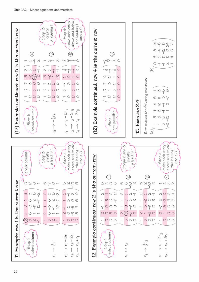
10. Strategy 2.1 Row-reducing a matrix
25
Unit LA2 Linear equations and matrices
26

Section 2 Rowreduction
27

Unit LA2 Linear equations and matrices
Further exercisesExercise 2.6 Which of the following are row-reduced matrices?
(a)
0 0 1 51 0 0 70 1 0 7
(b)
1 14 0 230 0 1 440 0 0 0
(c)
1 0 0 0 0 10 0 1 0 0 00 0 0 0 1 00 0 0 0 0 00 0 0 0 0 0
(d)
0 1 0 −3 120 0 1 0 70 0 0 1 20 0 0 0 00 0 0 0 0
(e)
(
0 1 1
70 −6 24 −3
7
0 0 0 1 3 −2
7
1
7
)
(f)
(
0 0 0 00 0 0 0
)
Exercise 2.7 Solve the systems of linear equations corresponding to thefollowing row-reduced augmented matrices. (Assume that the unknownsare x1, x2, . . ..)
(a)
1 0 0 70 1 0 −60 0 1 5
(b)
1 1
70 1
0 0 1 3
0 0 0 0
(c)
1 0 4 0 00 1 −3 0 00 0 0 1 0
(d)
1 3 0 −2 0 00 0 1 2 1 00 0 0 0 0 1
(e)
1 0 −5 0 40 1 −7 3 120 0 0 0 00 0 0 0 0
Exercise 2.8 Solve each of the following systems of linear equations byreducing its augmented matrix to row-reduced form.
(a)
3x − 11y − 3z = 32x − 6y − 2z = 15x − 17y − 6z = 24x − 8y = 7
(b)
a − 4c − 2d = −1a + 2b − 2c + 4d = 6
2a + 4b − 3c + 9d = 92a + b − 5c + d = −4
(c)
2x1 + 2x2 − 5x3 + 6x4 + 10x5 = −22x1 + 2x2 − 6x3 + 6x4 + 8x5 = 02x1 − x3 + 2x4 + 7x5 = 7x1 + 2x2 − 5x3 + 5x4 + 4x5 = −3
28

Section 3 Matrix algebra
3 Matrix algebra
After working through this section, you should be able to:
(a) perform the matrix operations of addition, multiplication andtransposition;
(b) recognise the following types of matrix: square, zero, diagonal,lower-triangular, upper-triangular, identity, symmetric;
(c) express a system of simultaneous linear equations in matrix form.
Earlier, we saw how an augmented matrix concisely represents a system of Subsection 2.1
simultaneous linear equations.
A matrix of size m× n has m rows and n columns. An n× n matrix iscalled a square matrix. The entry in the ith row and jth column of amatrix A is called the (i, j)-entry, often denoted by aij. In general, wewrite A or (aij) to denote a matrix:
A =
a11 a12 · · · a1na21 a22 · · · a2n...
......
am1 am2 · · · amn
= (aij).
Exercise 3.1 Write down the size of each of the following matrices.Which matrices are square? What is the (2, 3)-entry in each matrix?
(a)
(
3 −4 2 6−1 0 5 1
)
(b)
1 3 7−1 10 02 4 1
(c)
(
2 1−3 7
)
Two m× n matrices A = (aij) and B = (bij) are equal if aij = bij for allvalues of i and j.
Definition Two matrices A and B of the same size are equal if alltheir corresponding entries agree. We write A = B.
Thus
(
1 2 34 5 6
)
is not equal to
(
1 2 14 5 6
)
as the (1, 3)-entries differ,
and
(
1 1 11 1 1
)
is not equal to
1 11 11 1
as the matrices are different
sizes. A matrix of size 1× 1 comprises just a single entry; we often omitthe brackets and identify such matrices with ordinary numbers—scalars;for example, we identify the matrix (5) with the number 5.
We call a matrix with just one column a column matrix, and a matrix withjust one row a row matrix. For example,
123
is a column matrix and(
1 2 3 4)
is a row matrix.
29

Unit LA2 Linear equations and matrices
3.1 Matrix additionLet a = (a1, a2) and b = (b1, b2) be two vectors in R
2. Their sum is defined Unit LA1, Subsection 2.2.
to be the vector
a+ b = (a1 + b1, a2 + b2).
For example,
(1, 2) + (−2, 3) = (1 + (−2), 2 + 3) = (−1, 5).
We add matrices in precisely the same way; that is, by addingcorresponding entries. For example,
(
1 01 2
)
+
(
2 −10 1
)
=
(
1 + 2 0 + (−1)1 + 0 2 + 1
)
=
(
3 −11 3
)
and(
2 1 53 0 1
)
+
(
−2 4 21 3 2
)
=
(
0 5 74 3 3
)
.
It is clear that only matrices of the same size can be added together. Forexample, the following is meaningless:
(
1 2 34 5 6
)
+
1 23 45 6
.
We now write down a general formula for the addition of two matrices.
Definition The sum of two m× n matrices A = (aij) and B = (bij)is the m× n matrix A+B = (aij + bij) given by
A+B =
a11 + b11 a12 + b12 · · · a1n + b1na21 + b21 a22 + b22 · · · a2n + b2n
......
...am1 + bm1 am2 + bm2 · · · amn + bmn
.
Exercise 3.2 Evaluate the following matrix sums, where possible.
(a)
(
1 −3−2 54
)
+
(
2 04 1
)
(b)
(
2 04 1
)
+
(
1 −3−2 54
)
(c)
1 21 04 1
+
1 2 21 3 1
−2 4 5
(d)
0 6 −21 8 20 3 4
+
1 2 91 0 43 −4 1
In Exercise 3.2, parts (a) and (b) give the same answer. The commutativelaw, a+ b = b+ a, holds for the addition of scalars, as does the associativelaw, a+ (b+ c) = (a+ b) + c, for all a, b, c ∈ R. Since matrix addition isdefined in terms of addition of scalars, matrix addition is bothcommutative and associative.
Theorem 3.1 For all matrices A, B and C of the same size,
A+B = B+A (commutative law),
A+ (B+C) = (A+B) +C (associative law).
30

Section 3 Matrix algebra
Proof Let A = (aij) and B = (bij). To prove the commutative law, weadd the corresponding entries of these two matrices.
The (i, j)-entry of the matrix A+B is aij + bij , and that of B+A isbij + aij .
Since aij and bij are scalars, aij + bij = bij + aij . Thus
A+B = (aij + bij) = (bij + aij) = B+A.
We ask you to prove the associative law in Exercise 3.3.
Exercise 3.3 Prove the associative law: for all matrices A, B and C
of the same size,
A+ (B+C) = (A+B) +C.
Zero matrix
We have seen that matrices can be added in a way analogous to addition ofscalars. There is a type of matrix that corresponds to the number 0,namely, the zero matrix, which, as its name suggests, is a matrix of 0s. Itis denoted by 0m,n, or by 0 when it is clear from the context which size ofmatrix is intended.
Definition The m× n zero matrix 0m,n is the m× n matrix inwhich all entries are 0.
The following are all examples of zero matrices:
(
00
)
,(
0 0 0)
,
0 0 0 00 0 0 00 0 0 0
and
0 0 · · · 00 0 · · · 0...
......
0 0 · · · 0
.
The following exercise shows that the zero matrix acts in the same way asthe number 0 under the operation of addition. The zero matrix is theidentity element for the operation of matrix addition.
Exercise 3.4 Show that A+ 0 = A for any matrix A = (aij).
Definition The negative of an m× n matrix A = (aij) is the m× nmatrix
−A = (−aij).
For example, if
A =
(
1 −2 3−4 5 −6
)
,
then
−A =
(
−1 2 −34 −5 6
)
.
31

Unit LA2 Linear equations and matrices
The negative of a matrix acts in the same way as the negative of a numberunder the operation of addition.
Theorem 3.2 Let A be a matrix. Then
A+ (−A) = (−A) +A = 0.
Proof Let A = (aij), so −A = (−aij). We add corresponding entries:the (i, j)-entry of the matrix A+ (−A) is aij + (−aij) = 0. Thus thematrix A+ (−A) is the zero matrix 0.
Matrix addition is commutative, so (−A) +A = A+ (−A). Thus(−A) +A is also the zero matrix 0.
The m× n matrix −A is the additive inverse of the m× n matrix A.Since the four group axioms The group axioms were defined
in Unit GTA1.G1 closure, G2 identity, G3 inverses, G4 associativity
are satisfied, the set of m× n matrices under the operation of matrixaddition forms a group.
Using the negative of a matrix, we can subtract matrices:
A−B = A+ (−B).
Exercise 3.5 Evaluate the following matrix differences, wherepossible.
(a)
(
3 02 7
)
−
10 31 515 12
(b)
(
5 8 127 2 −1
)
−
(
3 10 24 9 21
)
3.2 Multiplication of a matrix by a scalarMultiplication of a vector by a scalar generalises in the obvious way to Unit LA1, Subsection 2.2.
matrices. To multiply the vector a = (a1, a2) by the scalar k, we multiplyeach entry in turn by k; this gives
ka = (ka1, ka2).
Similarly, to multiply a matrix by a scalar k, we multiply each entry by k.For example,
3
(
1 2 34 5 6
)
=
(
3 6 912 15 18
)
, −1
2
(
−4 20 −6
)
=
(
2 −10 3
)
.
Definition The scalar multiple of an m× n matrix A = (aij) by ascalar k is the m× n matrix
kA =
ka11 ka12 · · · ka1nka21 ka22 · · · ka2n...
......
kam1 kam2 · · · kamn
= (kaij).
Notice that (−1)A = −A and 0A = 0.
32

Section 3 Matrix algebra
Exercise 3.6 Let
A =
5 −32 3
−1 0
and B =
2 1−2 −73 5
.
Evaluate the following.
(a) 4A (b) 4B (c) 4A+ 4B (d) 4(A+B)
You should have obtained the same answer for parts (c) and (d) ofExercise 3.6. In fact, we have the following general result.
Theorem 3.3 For all matrices A and B of the same size, and all You are asked to proveTheorem 3.3 in Exercise 3.16.scalars k, the distributive law holds; that is,
k(A+B) = kA+ kB.
3.3 Matrix multiplicationYou have seen that the addition of matrices generalises the addition of Subsection 3.1
scalars and of vectors. In Unit LA1, Subsection 3.1, we introduced amethod of ‘multiplying’ vectors—the dot product. Let a = (a1, a2, a3) andb = (b1, b2, b3) be two vectors in R
3. Then
a . b = a1b1 + a2b2 + a3b3.
Matrix multiplication is a generalisation of this idea.
To form the product of two matrices A and B, we combine the rows of Awith the columns of B. The (i, j)-entry of the product AB is obtained bymultiplying the entries in the ith row of A with the corresponding entriesin the jth column of B, and summing the products obtained.
For example, let
A =
(
1 2 34 5 6
)
and B =
1 2 34 5 67 8 9
.
To obtain the (1, 2)-entry of the product AB, we combine the first row of One way to remember how tomultiply matrices A and B is topicture running along the rowsof A and then diving down thecolumns of B.
A with the second column of B: we multiply together the first entry of thefirst row of A and the first entry of the second column of B, then multiplytogether the second entries of each, and then the third entries, finallyadding these three numbers. The (1, 2)-entry of AB is thus
(1× 2) + (2× 5) + (3× 8) = 2 + 10 + 24 = 36.
To obtain the (2, 3)-entry of the product AB, we combine the second rowof A with the third column of B. The (2, 3)-entry of AB is
(4× 3) + (5× 6) + (6× 9) = 12 + 30 + 54 = 96.
We can compare the way in which we combined the first row of A and thesecond column of B with the dot product of two vectors:
(1, 2, 3) . (2, 5, 8) = (1× 2) + (2× 5) + (3× 8) = 36.
We therefore say that we take the dot product of the first row of A withthe second column of B to obtain the (1, 2)-entry of the product AB.
33

Unit LA2 Linear equations and matrices
Likewise, we take the dot product of the second row of A with the thirdcolumn of B to obtain the (2, 3)-entry of the product AB:
(4, 5, 6) . (3, 6, 9) = (4× 3) + (5× 6) + (6 × 9) = 96.
Exercise 3.7 Find the (2, 1)-entry of the product AB, for thematrices A and B given above.
To form the matrix product AB, we combine each row of A with eachcolumn of B. We therefore obtain 2× 3 entries in the product AB, so thismatrix has 2 rows and 3 columns. We have found three of the six entries,as highlighted below.
You should check the otherentries.=
1 2 3
4 5 6
1 2 3
4 5 6
7 8 9
30
66
36
81
42
96
Notice that we can form the product AB since the matrix A has the samenumber of entries in a row as the matrix B has in a column; that is, thenumber of columns of A is equal to the number of rows of B.
The product AB is not defined when the number of columns of thematrix A is not equal to the number of rows of the matrix B.
Definition The product of an m× n matrix A with an n× p Notice that the product AB hasthe same number of rows as thematrix A, and the same numberof columns as the matrix B.
matrix B is the m× p matrix AB whose (i, j)-entry is the dotproduct of the ith row of A with the jth column of B.
Schematically,
Example 3.1 Evaluate (where possible) the matrix products AB, where:
(a) A =
(
2 1−3 0
)
and B =
(
3 −2 01 1 4
)
;
(b) A =
(
2 1−3 0
)
and B =(
3 −2)
.
Solution
(a) The matrix A has 2 columns and the matrix B has 2 rows, so theproduct AB can be formed. Since A has 2 rows and B has 3 columns,AB has 2 rows and 3 columns.
To find the (1, 1)-entry of the product AB, we take the dot product of When evaluating a product ofmatrices, it is advisable to findthe entries systematically, eithercolumn by column, or row byrow. Here, we find the entriescolumn by column.
the first row of A with the first column of B:
(2× 3) + (1× 1) = 7.
Next, to find the (2, 1)-entry of AB, we take the dot product of thesecond row of A with the first column of B:
(−3× 3) + (0× 1) = −9.
34

Section 3 Matrix algebra
Together, these give the first column of the product AB:
To find the (1, 2)-entry of the product AB, we take the dot product ofthe first row of A with the second column of B:
(2×−2) + (1× 1) = −3.
Next, to find the (2, 2)-entry of AB, we take the dot product of thesecond row of A with the second column of B:
(−3×−2) + (0× 1) = 6.
We now have the second column of the product AB:
To find the (1, 3)-entry of the product AB, we take the dot product ofthe first row of A with the third column of B:
(2× 0) + (1× 4) = 4.
Next, to find the (2, 3)-entry of AB, we take the dot product of thesecond row of A with the third column of B:
(−3× 0) + (0× 4) = 0.
We now have the third column of the product AB:
Thus(
2 1−3 0
)(
3 −2 01 1 4
)
=
(
7 −3 4−9 6 0
)
.
(b) The matrix A has 2 columns and the matrix B has 1 row, so theproduct AB is not defined.
Exercise 3.8 Evaluate the following matrix products, where possible.
(a)
2 −10 31 2
(
32
)
(b)(
2 1)
(
1 60 2
)
(c)
2−41
(
3 24 −1
)
(d)
(
12
)
(
3 0 −4)
(e)
(
3 1 20 5 1
)
−2 0 11 3 04 1 −1
Earlier, we showed that the operation of matrix addition is both Subsection 3.1
commutative and associative.
35

Unit LA2 Linear equations and matrices
Exercise 3.9 Let
A =
(
1 13 2
)
and B =
(
1 42 1
)
.
Calculate the products AB and BA. Comment on your findings.
You should have obtained different answers for AB and BA inExercise 3.9; thus matrix multiplication is not commutative. This meansthat it is important to describe the matrix product carefully. We say thatAB is the matrix A multiplied on the right by the matrix B, or thematrix B multiplied on the left by the matrix A.
Matrix multiplication is associative; that is, the products (AB)C and The associativity of matrixmultiplication is proved ingeneral in Unit LA4.
A(BC) are equal (when they can be formed).
You have seen that the distributive law holds for multiplication of a matrixby a scalar. This law also holds for multiplication of a matrix by a matrix;that is, A(B+C) = AB+AC, whenever these products can be formed.
Diagonal and triangular matrices
The entries of a square matrix from the top left-hand corner to the bottomright-hand corner are the diagonal entries; the diagonal entries form the The main diagonal is sometimes
called the leading or principaldiagonal .
main diagonal of the matrix. For a square matrix A = (aij) of size n× n,the diagonal entries are
a11, a22, . . . , ann.
Definition A diagonal matrix is a square matrix each of whosenon-diagonal entries is zero.
For example, the following are diagonal matrices:
(
1 00 −2
)
and
3 0 00 −7 00 0 0
.
To see how diagonal matrices multiply, try the following exercise.
Exercise 3.10 Let
A =
(
1 00 7
)
, B =
(
−3 00 4
)
and C =
(
2 00 12
)
.
Evaluate the following products.
(a) AB (b) BA (c) ABC
Notice that the product of two diagonal matrices is another diagonalmatrix. Multiplying diagonal matrices is straightforward—the ith diagonalentry of the product is the product of the ith diagonal entries of thematrices being multiplied. Multiplication of diagonal matrices is thereforecommutative.
A square matrix with each entry below the main diagonal equal to zero iscalled an upper-triangular matrix . Similarly, a matrix with each entryabove the main diagonal equal to zero is called a lower-triangular matrix .A square row-reduced matrix is an upper-triangular matrix. A squarematrix that is both upper-triangular and lower-triangular is necessarily adiagonal matrix.
36

Section 3 Matrix algebra
Exercise 3.11 State which of the following matrices are diagonal,upper-triangular or lower-triangular.
(a)
1 1 10 2 20 0 3
(b)
(
9 00 0
)
(c)
0 0 10 1 21 2 3
(d)
(
1 01 0
)
Identity matrix
We have found that there are matrices corresponding to the number 0, thezero matrices 0m,n. There is also a matrix corresponding to the number 1,namely, the identity matrix, denoted by In. The subscript n indicates that The identity matrix is written
simply as I when the size is clearfrom the context.
the matrix is an n× n matrix.
Definition The identity matrix In is the n× n matrix
1 0 · · · 0 00 1 · · · 0 0...
.... . .
......
0 0 · · · 1 00 0 · · · 0 1
.
Each of the entries is 0 except those on the main diagonal, which areall 1.
For example, the identity matrices I2, I3 and I4 are
(
1 00 1
)
,
1 0 00 1 00 0 1
,
1 0 0 00 1 0 00 0 1 00 0 0 1
.
If we multiply a 3× 2 matrix on the left by I3 and then on the right by I2,we obtain
1 0 00 1 00 0 1
a bc de f
=
a bc de f
Here, a, b, c, d, e and f are anyreal numbers.
and
a bc de f
(
1 00 1
)
=
a bc de f
.
In both cases, the matrix is unchanged.
Theorem 3.4 Let A be an m× n matrix. Then You are asked to proveTheorem 3.4 in Exercise 3.17.
ImA = AIn = A.
37

Unit LA2 Linear equations and matrices
3.4 Transposition of matricesThere is a simple operation that we can perform on matrices. Thisoperation, called transposition or taking the transpose, entails Transposition of a square matrix
can be thought of as reflectingthe matrix in the main diagonal.
interchanging the rows with the columns of the matrix. Thus the transposeof the matrix A, denoted by AT , has the rows of A as its columns, takenin the same order. For example,
1 2 34 5 67 8 9
T
=
1 4 72 5 83 6 9
and
2 7−6 10 4
T
=
(
2 −6 07 1 4
)
.
Definition The transpose of an m× n matrix A is the n×mmatrix AT whose (i, j)-entry is the (j, i)-entry of A.
Exercise 3.12 Write down the transpose of each of the followingmatrices.
(a)
1 40 2
−6 10
(b)
2 1 20 3 −54 7 0
(c)(
10 4 6)
(d)
(
1 00 2
)
The identity matrix I is not changed by taking the transpose; that is,IT = I.
The rows of the matrix A form the columns of the matrix AT , and thecolumns of AT form the rows of (AT )T . Therefore the rows of A form therows of (AT )T ; that is, these two matrices are equal:
(AT )T = A.
Exercise 3.13 Let
A =
1 23 45 6
, B =
7 89 1011 12
and C =
(
1 01 1
)
.
(a) Find AT , BT and (A+B)T , and verify that
(A+B)T = AT +BT .
(b) Find CT and (AC)T , and discover an equation relating (AC)T ,
AT and CT .
The relationships satisfied by the matrices in Exercise 3.13 hold in general.We collect together these results for the transposition of matrices in thefollowing theorem.
Theorem 3.5 Let A and B be m× n matrices. Then the following We omit the proofs: (a) and (b)are straightforward to prove.results hold:
(a) (AT )T = A;
(b) (A+B)T = AT +BT .
Let A be an m× n matrix and B an n× p matrix. Then
(c) (AB)T = BTAT .
38

Section 3 Matrix algebra
Symmetric matrices
Some square matrices remain unchanged when transposed. These matricesare called symmetric matrices, since they are symmetrical about the maindiagonal.
Definition A square matrix A is symmetric if
AT = A.
The entries off the main diagonal of a diagonal matrix are all zero, so alldiagonal matrices are symmetric, as are the following:
3 1 11 3 11 1 3
,
(
1 11 1
)
,
1 2 3 42 5 6 73 6 8 94 7 9 10
,
(
−5 22 3
)
.
3.5 Matrix form of a system of linearequationsIn this subsection we show how a system of linear equations can beexpressed in matrix form as a product of matrices. This helps to explainwhy we multiply matrices in such an ‘odd way’.
Consider the system of simultaneous linear equations
x1 + 2x2 + 4x3 = 6,x2 + x3 = 1,
x1 + 3x2 + 5x3 = 10.
We can write this system as a matrix equation:
x1 + 2x2 + 4x3x2 + x3
x1 + 3x2 + 5x3
=
6110
.
Now the 3× 1 matrix on the left can be expressed as the product of twomatrices, namely, the 3× 3 matrix of the coefficients and the 3× 1 matrixof the unknowns:
x1 + 2x2 + 4x3x2 + x3
x1 + 3x2 + 5x3
=
1 2 40 1 11 3 5
x1x2x3
.
Thus we have the matrix equation
1 2 40 1 11 3 5
x1x2x3
=
6110
.
Similarly, we can express any system of simultaneous linear equations
a11x1 + a12x2 + · · · + a1nxn = b1,a21x1 + a22x2 + · · · + a2nxn = b2,...
......
...am1x1 + am2x2 + · · · + amnxn = bm,
as a matrix product.
39

Unit LA2 Linear equations and matrices
Let the matrix of coefficients be A, the coefficient matrix of the system,that is,
A =
a11 a12 · · · a1na21 a22 · · · a2n...
......
am1 am2 · · · amn
.
Let the matrix of unknowns be x, and let the matrix of constant termsbe b, so
x =
x1x2...xn
and b =
b1b2...bm
.
The system can then be expressed in matrix form as
Ax = b,
or in full as
a11 a12 · · · a1na21 a22 · · · a2n...
......
am1 am2 · · · amn
x1x2...xn
=
b1b2...bm
.
Further exercises
Exercise 3.14 Let A =
(
1 63 −4
)
and B =
(
2 −30 7
)
. Evaluate the
following.
(a) A+B (b) A−B (c) B−A (d) AB (e) BA
(f) A2 (g) AT (h) BT (i) ATBT
Exercise 3.15 Suppose that we are given matrices of the following sizes:
A : 2× 1, B : 4× 3, C : 3× 2, D : 1× 4,
E : 3× 3, F : 3× 4, G : 2× 4.
Which of the following expressions are defined? Give the size of theresulting matrix for those that are defined.
(a) FB+E (b) GFT −ADB (c) BF− (FB)T
(d) C(AD+G) (e) (CA)TD (f) ETBTGTCT
Exercise 3.16 Prove the distributive law, that for all matrices A and B of This is Theorem 3.3.
the same size, and all scalars k,
k(A+B) = kA+ kB.
Exercise 3.17 Let A = (aij) be an m× n matrix. Prove that ImA = A This is Theorem 3.4.
and AIn = A.
Hint: Notice that the entries in the ith row of Im are all 0 except the entryin the ith position, which is 1.
40

Section 4 Matrix inverses
4 Matrix inverses
After working through this section, you should be able to:
(a) understand what is meant by an invertible matrix;
(b) understand that the set of n× n invertible matrices forms a groupunder matrix multiplication;
(c) determine whether or not a given matrix is invertible and, if it is,find its inverse;
(d) state the relationship between the invertibility of a square matrixand the number of solutions of a system of linear equations withthat square matrix as its coefficient matrix;
(e) understand the connections between elementary row operationsand elementary matrices.
4.1 Matrix inversesIn Section 3 we saw that many of the properties of ordinary arithmetichave analogues in matrix algebra. We now consider the extent to which afurther important property of ordinary arithmetic is mirrored in matrixalgebra. You are familiar with the fact that, for each non-zero realnumber a, there exists a number b, called the reciprocal or multiplicative For example, the reciprocal of 4
is 1
4.inverse of a, such that
ab = 1 and ba = 1.
Each non-zero real number a has exactly one reciprocal, and we denote itby a−1 or 1/a.
The role played by the number 1 in ordinary arithmetic is played in matrixalgebra by the identity matrix I; therefore we make the following definition.
Definition Let A be a square matrix, and suppose that there existsa matrix B of the same size such that
AB = I and BA = I. You need both these equationsfor B to be the inverse of A.One alone is not enough.Then B is an inverse of A.
Notice that we restrict the definition to square matrices. It can be provedthat if A is not a square matrix, then AB and BA cannot both be identitymatrices—so the definition cannot be extended to non-square matrices.
For example,(
3 −1−5 2
)
is an inverse of
(
2 15 3
)
since(
2 15 3
)(
3 −1−5 2
)
=
(
1 00 1
)
and(
3 −1−5 2
)(
2 15 3
)
=
(
1 00 1
)
.
41

Unit LA2 Linear equations and matrices
Similarly,
−1 −5 −20 2 1
−2 1 1
is an inverse of
1 3 −1−2 −5 14 11 −2
since
1 3 −1−2 −5 14 11 −2
−1 −5 −20 2 1
−2 1 1
=
1 0 00 1 00 0 1
and
−1 −5 −20 2 1
−2 1 1
1 3 −1−2 −5 14 11 −2
=
1 0 00 1 00 0 1
.
Just as a real number has at most one reciprocal, a square matrix has atmost one inverse, as we now prove.
Theorem 4.1 A square matrix has at most one inverse.
Proof Let A be a square matrix, and suppose that B and C are bothinverses of A. Then AB = I and CA = I.
Multiplying the equation AB = I on the left by C, we have
C(AB) = CI = C,
while multiplying the equation CA = I on the right by B gives This shows us why we need bothAB = I and BA = I in thedefinition on page 41.(CA)B = IB = B.
Since matrix multiplication is associative, it follows that B = C.
Now, every non-zero real number has a reciprocal, so it is natural to askwhether or not every non-zero square matrix has an inverse. The next Certainly a square zero matrix
has no inverse (just as the realnumber 0 has no reciprocal).This is easy to see: if 0 is asquare zero matrix, then anyproduct of 0 and another matrixis a zero matrix, so there is nomatrix B such that 0B = I.
exercise demonstrates that the answer to this question is no—it gives anexample of a non-zero square matrix with no inverse.
Exercise 4.1 Let A =
(
1 −1−1 1
)
.
Prove that there is no matrix B =
(
a bc d
)
such that AB = I.
In fact, there are many non-zero square matrices with no inverse. The nexttheorem gives an infinite class of such matrices.
Theorem 4.2 A square matrix with a zero row has no inverse.
Proof Let A be a square matrix one of whose rows, say row i, is a zerorow. Then if B is any matrix of the same size as A, the (i, i)-entry of AB
is 0, since it is equal to the dot product of row i of A (a zero row) withcolumn i of B. But the (i, i)-entry of I is 1, which shows that there is nomatrix B such that AB = I. Hence A has no inverse.
42

Section 4 Matrix inverses
Definition A square matrix that has an inverse is invertible.
We denote the unique inverse of an invertible matrix A by A−1. Thus, forany invertible matrix A,
AA−1 = I and A−1A = I.
Notice from these equations that if A is an invertible matrix, then A−1 isalso invertible, with inverse A; that is,
(A−1)−1 = A.
In other words, A and A−1 are inverses of each other. This is similar to inverses in R,where (a−1)−1 = a.
The next example and the following exercises give some other useful factsabout matrix inverses.
Example 4.1 Let A be an invertible matrix. Prove that AT is invertible, We introduced AT , thetranspose of A, inSubsection 3.4.
and that (AT )−1 = (A−1)T .
Solution To prove that AT is invertible, with inverse (A−1)T , we haveto show that
AT (A−1)T = I and (A−1)TAT = I.
ButRecall from Subsection 3.4 that
(AB)T = BTAT .AT (A−1)T = (A−1A)T = IT = I,
and, similarly,
(A−1)TAT = (AA−1)T = IT = I.
The required result follows.
Exercise 4.2 Prove that I is invertible, and that I−1 = I.
Exercise 4.3 Let A and B be invertible matrices of the same size.Prove that AB is invertible, and that (AB)−1 = B−1A−1.
Notice the reversal of the order of the matrices in the identity
(AB)−1 = B−1A−1.
The result of Exercise 4.3 extends to products of any number of matrices.
Theorem 4.3 Let A1,A2, . . . ,Ak be invertible matrices of the same This can be proved using theresult of Exercise 4.3 andmathematical induction.
size. Then the product A1A2 · · ·Ak is invertible, with
(A1A2 · · ·Ak)−1 = A−1
k A−1
k−1· · ·A−1
1.
Using the results of the above exercises, we can show that the set of allinvertible matrices of a particular size forms a group under matrix The group axioms were defined
in Unit GTA1.multiplication.
Theorem 4.4 The set of all invertible n× n matrices forms a group The set of all n× n matricesdoes not form a group undermatrix multiplication: it fails tosatisfy the axiom G3 inverses,since, for example, the n× nzero matrix has no inverse.
under matrix multiplication.
43

Unit LA2 Linear equations and matrices
Proof We must check that the four group axioms hold.
Exercise 4.3 tells us that the group axiom G1 closure holds for this set.
Exercise 4.2 shows that I is a member of the set, so the set contains anidentity element. In other words, the axiom G2 identity holds.
Each matrix in the set has an inverse, and this inverse is itself invertible Remember, (A−1)−1 = A.
and therefore also in the set; so the axiom G3 inverses holds.
Finally, we know from Section 3 that matrix multiplication is associative,so the axiom G4 associativity holds.
4.2 Invertibility TheoremThe following two questions may already have occurred to you as youworked through the previous subsection. First, how can we determinewhether or not a given square matrix is invertible? Second, if we knowthat a matrix is invertible, how can we find its inverse? The next theoremanswers both questions.
Theorem 4.5 Invertibility Theorem
(a) A square matrix is invertible if and only if its row-reduced formWe prove the InvertibilityTheorem in Subsection 4.5.
is I.
(b) Any sequence of elementary row operations that transforms amatrix A to I also transforms I to A−1.
To illustrate this theorem, consider the matrix A =
(
1 32 9
)
. Suppose
that we wish to determine whether or not A is invertible and, if it is, tofind A−1.
Below, on the left, we row-reduce A in the usual way. On the right, weperform the same sequence of elementary row operations on the 2× 2identity matrix.
r1r2
(
1 32 9
)
r1r2
(
1 00 1
)
r2 → r2 − 2r1
(
1 30 3
)
r2 → r2 − 2r1
(
1 0−2 1
)
r2 →1
3r2
(
1 30 1
)
r2 →1
3r2
(
1 0−2
3
1
3
)
r1 → r1 − 3r2(
1 00 1
)
r1 → r1 − 3r2(
3 −1−2
3
1
3
)
The row-reduced form of A is I, so we conclude from the first part of theInvertibility Theorem that A is an invertible matrix.
By the second part of the Invertibility Theorem, the final matrix on theright above must be A−1; that is,
You should check that thismatrix is indeed the inverseof A.
A−1 =
(
3 −1−2
3
1
3
)
.
When we apply the Invertibility Theorem to find the inverse of amatrix A, we have to perform the same sequence of elementary rowoperations on both A and I. We can do this conveniently in the following
44

Section 4 Matrix inverses
way. We begin by writing A and I alongside each other, separated by avertical line, giving a larger matrix which we may denote by (A | I). Wethen row-reduce (A | I) in the usual way. When we do this, the abovecalculation looks like this:
r1r2
(
1 3 1 02 9 0 1
)
r2 → r2 − 2r1
(
1 3 1 00 3 −2 1
)
r2 →1
3r2
(
1 3 1 00 1 −2
3
1
3
)
r1 → r1 − 3r2(
1 0 3 −10 1 −2
3
1
3
)
.
Thus the Invertibility Theorem gives us the following strategy.
Strategy 4.1 To determine whether or not a given square matrix A You may find it helpful toremember the following scheme:
(A | I)
↓
(I | A−1).
is invertible, and find its inverse if it is.
Write down (A | I), and row-reduce it until the left half is inrow-reduced form.
• If the left half is the identity matrix, then the right half is A−1.
• Otherwise, A is not invertible.
Remark Strategy 4.1 is most useful for matrices of size 3× 3 and larger.In Section 5 we give a quick method for determining whether or not a2× 2 matrix is invertible, and for writing down its inverse if it is.
Example 4.2 Determine whether or not each of the following matrices isinvertible, and find the inverse if it exists.
(a)
1 1 2−1 0 −43 2 10
(b)
1 3 53 1 72 4 8
Solution We use Strategy 4.1.
(a) We form the matrix (A | I), and row-reduce it in the usual way.
r1r2r3
1 1 2 1 0 0−1 0 −4 0 1 03 2 10 0 0 1
r2 → r2 + r1r3 → r3 − 3r1
1 1 2 1 0 00 1 −2 1 1 00 −1 4 −3 0 1
r1 → r1 − r2
r3 → r3 + r2
1 0 4 0 −1 00 1 −2 1 1 00 0 2 −2 1 1
r3 →1
2r3
1 0 4 0 −1 00 1 −2 1 1 00 0 1 −1 1
2
1
2
r1 → r1 − 4r3r2 → r2 + 2r3
1 0 0 4 −3 −20 1 0 −1 2 10 0 1 −1 1
2
1
2
45

Unit LA2 Linear equations and matrices
The left half has been reduced to I, so the given matrix is invertible;its inverse is given by the right half, that is,
4 −3 −2−1 2 1−1 1
2
1
2
.
(b) We row-reduce (A | I).
r1r2r3
1 3 5 1 0 03 1 7 0 1 02 4 8 0 0 1
r2 → r2 − 3r1r3 → r3 − 2r1
1 3 5 1 0 00 −8 −8 −3 1 00 −2 −2 −2 0 1
r2 → −1
8r2
1 3 5 1 0 0
0 1 1 3
8−1
80
0 −2 −2 −2 0 1
r1 → r1 − 3r2
r3 → r3 + 2r2
1 0 2 −1
8
3
80
0 1 1 3
8−1
80
0 0 0 −5
4−1
41
The left half is now in row-reduced form, but is not the identitymatrix. Therefore the given matrix is not invertible.
Remark If it becomes clear while you are row-reducing (A | I) that theleft half will not reduce to the identity matrix (for example, if a zero rowappears in the left half), then you can stop the row-reduction immediately,and conclude that A is not invertible. There is no point in continuing untilthe left half is in row-reduced form.
Exercise 4.4 Use Strategy 4.1 to determine whether or not each ofthe following matrices is invertible, and find the inverse if it exists.
(a)
(
2 44 1
)
(b)
1 1 −42 1 −6
−3 −1 9
(c)
2 4 61 2 45 10 5
4.3 Invertibility and systems of linearequationsWe can use matrix inverses to give us another method for solving certainsystems of linear equations.
Consider the system We solved this system byGauss–Jordan elimination inExample 1.1.
{
2x + 4y = 10,4x + y = 6.
This system may be expressed in matrix form as(
2 44 1
)(
xy
)
=
(
106
)
.
The coefficient matrix
(
2 44 1
)
is invertible, with inverse
(
− 1
14
2
7
2
7−1
7
)
. See Exercise 4.4(a).
46

Section 4 Matrix inverses
Multiplying both sides of the matrix form of the system on the left by theinverse of the coefficient matrix, we obtain
(
− 1
14
2
7
2
7−1
7
)
(
2 44 1
)(
xy
)
=
(
− 1
14
2
7
2
7−1
7
)
(
106
)
,
that is,(
1 00 1
)(
xy
)
=
(
12
)
,
or(
xy
)
=
(
12
)
.
So the system has the unique solution
(
xy
)
=
(
12
)
; that is, x = 1, y = 2.
In general, suppose that Ax = b is the matrix form of a system of linearequations, and that the coefficient matrix A is invertible. Then we canmultiply both sides of the equation Ax = b on the left by A−1 to yieldA−1Ax = A−1b; that is, x = A−1b. It seems, then, that the system hasthe unique solution x = A−1b.
However, we have to be careful before making this claim. Whenever wemanipulate an equation in order to solve it, we have to be sure that themanipulation yields a second equation equivalent to the first (otherwise thetwo equations might have different solution sets).
In this case, we have to be sure that
Ax = b if and only if x = A−1b.
We showed above that if Ax = b, then multiplying both sides on the leftby A−1 yields x = A−1b; in other words, we proved that Ax = b impliesx = A−1b. It remains to prove that x = A−1b implies Ax = b, andfortunately this is just as easy: if x = A−1b, then multiplying both sidesof this equation on the left by A yields Ax = AA−1b; that is, Ax = b.
So multiplying both sides of Ax = b on the left by A−1 does yield anequivalent equation. We have proved the following theorem.
Theorem 4.6 Let A be an invertible matrix. Then the system oflinear equations Ax = b has the unique solution x = A−1b.
Exercise 4.5 Use Theorem 4.6 to solve the following system of linearequations:
x + y + 2z = 1,−x − 4z = 2,3x + 2y + 10z = −1.
Hint: The inverse of the matrix
1 1 2−1 0 −43 2 10
is
4 −3 −2−1 2 1−1 1
2
1
2
. We calculated this inverse inExample 4.2(a).
47

Unit LA2 Linear equations and matrices
Remark In general, it is worth using the method of Theorem 4.6 only if To use the method ofTheorem 4.6 to solve Ax = b,where A is an n× n invertiblematrix, we first invert A. Thisinvolves row-reducing the matrix(A | I). We then calculate thematrix product A−1b. Themethod of Section 2 involvesonly row-reducing the matrix(A | b).
we have already calculated the inverse of the coefficient matrix. If we donot know the inverse of the coefficient matrix, then the Gauss–Jordanelimination method of Section 2 is usually quicker.
Theorem 4.6 shows, in particular, that if the coefficient matrix A of asystem of linear equations Ax = b is invertible, then the system has aunique solution. The converse of this result is also true—we prove this inthe next theorem.
This theorem gives some important relationships between the invertibilityof a matrix and the number of solutions of systems of linear equations withthat matrix as coefficient matrix. The theorem states that the threeconditions are equivalent : any one of the conditions implies any other one.
Theorem 4.7 Let A be an n× n matrix. Then the followingstatements are equivalent.
(a) A is invertible.
(b) The system Ax = b has a unique solution for each n× 1matrix b.
(c) The system Ax = 0 has only the trivial solution.
Proof We show that (a)⇒ (b), (b)⇒ (c) and (c)⇒ (a), which shows thatthe conditions are equivalent.
(a) ⇒ (b)Suppose that A is an invertible n× n matrix. Then, by Theorem 4.6, forany n× 1 matrix b, the system Ax = b has the unique solution x = A−1b.
(b) ⇒ (c)Suppose that the system Ax = b has a unique solution for each n× 1matrix b. Then, in particular, the homogeneous system Ax = 0 has aunique solution. But every homogeneous system has the trivial solution;thus this unique solution must be the trivial one.
(c) ⇒ (a)Suppose that the system Ax = 0 has only the trivial solution. Thenrow-reducing the augmented matrix
a11 a12 · · · a1n 0a21 a22 · · · a2n 0...
......
...am1 am2 · · · amn 0
of the system must yield
1 0 · · · 0 00 1 · · · 0 0...
.... . .
......
0 0 · · · 1 0
,
since this is the row-reduced matrix that corresponds to each unknownbeing 0. If we now ignore the last column of each of the matricesappearing in this row-reduction, we are left with a reduction of A to I.Hence, by the Invertibility Theorem, A is invertible.
48

Section 4 Matrix inverses
4.4 Elementary matricesIn this subsection we introduce and study a class of square matricesassociated with elementary row operations.
We shall use these matrices and their properties in Subsection 4.5, to helpus prove the Invertibility Theorem. We shall also find them useful later.
Consider the following matrices:
0 1 01 0 00 0 1
,
1 0 00 5 00 0 1
,
1 0 00 1 00 2 1
.
They are obtained by performing, on the 3× 3 identity matrix, theelementary row operations r1 ↔ r2, r2 → 5r2 and r3 → r3 + 2r2,respectively.
Definition A matrix obtained by performing an elementary rowoperation on an identity matrix is an elementary matrix.
The elementary row operation that is performed to obtain an elementarymatrix from an identity matrix is called the elementary row operationassociated with that elementary matrix.
We now demonstrate the most important property of elementary matrices.Below, we show the effect of multiplying the matrix
A =
1 2 3 45 6 7 89 10 11 12
on the left by each of the above elementary matrices. Notice that in eachcase, the resulting matrix is precisely the matrix that is obtained when therow operation associated with the elementary matrix is performed on A.
0 1 01 0 00 0 1
1 2 3 45 6 7 89 10 11 12
=
5 6 7 81 2 3 49 10 11 12
elementary matrix A matrix obtained whenassociated with r1 ↔ r2
r1 ↔ r2 is performed on A
1 0 00 5 00 0 1
1 2 3 45 6 7 89 10 11 12
=
1 2 3 425 30 35 409 10 11 12
elementary matrix A matrix obtained whenassociated with r2 → 5r2
r2 → 5r2 is performed on A
1 0 00 1 00 2 1
1 2 3 45 6 7 89 10 11 12
=
1 2 3 45 6 7 819 22 25 28
elementary matrix A matrix obtained whenassociated with r3 → r3 + 2r2r3 → r3 + 2r2 is performed on A
There is nothing special about the above elementary matrices, or aboutthe above matrix A. In the next exercise, you will find that otherelementary matrices behave similarly.
49

Unit LA2 Linear equations and matrices
Exercise 4.6 Let A =
(
1 2 33 2 1
)
and B =
1 23 45 67 8
.
(a) Write down the 2× 2 elementary matrix associated with the This elementary matrix is theone obtained when r1 → 5r1 isperformed on the 2× 2 identitymatrix.
elementary row operation r1 → 5r1.
Multiply A on the left by this elementary matrix, and check thatthe resulting matrix is the same as the matrix obtained whenr1 → 5r1 is performed on A.
(b) Write down the 4× 4 elementary matrix associated with theelementary row operation r2 → r2 + 3r4.
Multiply B on the left by this elementary matrix, and check thatthe resulting matrix is the same as the matrix obtained whenr2 → r2 + 3r4 is performed on B.
In general, we have the following theorem.
Theorem 4.8 Let E be an elementary matrix, and let A be any We omit the proof.
matrix with the same number of rows as E. Then the product EA is A must have the same numberof rows as E for the product EAto be defined.
the same as the matrix obtained when the elementary row operationassociated with E is performed on A.
Theorem 4.8 tells us that if we perform an elementary row operation on amatrix A with m rows, then the resulting matrix is EA, where E is them×m elementary matrix associated with the row operation.
What happens if we perform a sequence of k elementary row operations ona matrix A with m rows? Let E1,E2, . . . ,Ek be the m×m elementarymatrices associated with the row operations in the sequence, in the sameorder. The first row operation is performed on A, producing the matrixE1A; the second row operation is then performed on this matrix,producing the matrix E2(E1A) = E2E1A; and so on. After the wholesequence of k row operations has been performed, the resulting matrix isEkEk−1 · · ·E2E1A. The order of the elementary
matrices in the matrix productis the reverse of the order inwhich their associated rowoperations are performed.
This fact will be useful later, and we record it as a corollary toTheorem 4.8.
Corollary to Theorem 4.8 Let E1,E2, . . . ,Ek be the m×melementary matrices associated with a sequence of k elementary rowoperations carried out on a matrix A with m rows, in the same order.Then, after the sequence of row operations has been performed, theresulting matrix is
EkEk−1 · · ·E2E1A.
For example, earlier we performed the sequence of row operations
r2 → r2 − 2r1, r2 →1
3r2, r1 → r1 − 3r2,
on the matrix
(
1 32 9
)
, producing the matrix
(
1 00 1
)
.
50

Section 4 Matrix inverses
By the above corollary,
You should check this byevaluating the product on theright-hand side.
(
1 00 1
)
=
(
1 −30 1
)(
1 00 1
3
)(
1 0−2 1
)(
1 32 9
)
.
We now explore some other useful connections between elementary rowoperations and elementary matrices. We begin by introducing a furtherproperty of elementary row operations.
In the following example, the second elementary row operation undoes theeffect of the first.
r1r2
(
1 2 34 5 6
)
r2 → r2 + 3r1
(
1 2 37 11 15
)
r2 → r2 − 3r1
(
1 2 34 5 6
)
In fact, given any elementary row operation, it is easy to write down aninverse elementary row operation that undoes the effect of the first, assummarised in the following table.
Elementary row operation Inverse elementary row operation
ri ↔ rj ri ↔ rjri → c ri (c 6= 0) ri → (1/c) riri → ri + c rj ri → ri − c rj
Exercise 4.7 Write down the inverse of each of the followingelementary row operations. Check your answer in each case bycarrying out the sequence of two row operations on the matrix(
1 2 34 5 6
)
.
(a) r1 → r1 − 2r2 (b) r1 ↔ r2 (c) r2 → −3r2
Note from the table that if two elementary row operations are such thatthe second is the inverse of the first, then the first is the inverse of thesecond—so it makes sense to say that they are inverses of each other, orthat they form an inverse pair. For example, the inverse of r2 → r2 + 3r1is r2 → r2 − 3r1, and the inverse of r2 → r2 − 3r1 is r2 → r2 − (−3)r1, thatis, r2 → r2 + 3r1. So r2 → r2 + 3r1 and r2 → r2 − 3r1 are inverses of eachother.
Now consider the following pair of 2× 2 elementary matrices associatedwith the inverse pair of elementary row operations r2 → r2 + 3r1 andr2 → r2 − 3r1:
(
1 03 1
)
,
(
1 0−3 1
)
.
These two matrices are themselves inverses of each other, as we can easilycheck:
(
1 03 1
)(
1 0−3 1
)
=
(
1 00 1
)
and(
1 0−3 1
)(
1 03 1
)
=
(
1 00 1
)
.
51

Unit LA2 Linear equations and matrices
This connection between inverse pairs of elementary row operations andinverse pairs of elementary matrices holds in general.
Theorem 4.9 Let E1 and E2 be elementary matrices of the same sizewhose associated elementary row operations are inverses of eachother. Then E1 and E2 are inverses of each other.
Proof In this proof we refer to the row operations associated with E1
and E2 as row operation 1 and row operation 2, respectively.
By the corollary to Theorem 4.8, E2E1I is the matrix produced when rowoperations 1 and 2 are performed, in that order, on I. Similarly, E1E2I isthe matrix produced when row operations 2 and 1 are performed, in thatorder, on I. But each of these two row operations undoes the effect of theother, so E2E1I = I and E1E2I = I; that is, E2E1 = I and E1E2 = I.Thus E1 and E2 are inverses of each other.
Theorem 4.9 has the following corollary.
Corollary to Theorem 4.9 Every elementary matrix is invertible,and its inverse is also an elementary matrix.
Proof Let E be an elementary matrix. Then E has an associatedelementary row operation. This associated elementary row operation hasan inverse operation, and the elementary matrix of the same size as Eassociated with this inverse operation is the inverse of E, byTheorem 4.9.
Exercise 4.8 Use the method suggested by the proof of the above
corollary to find the inverse of the elementary matrix
2 0 00 1 00 0 1
.
4.5 Proof of the Invertibility TheoremWe are now ready to prove the Invertibility Theorem, using elementarymatrices and their properties. We first remind you of the theorem.
Theorem 4.5 Invertibility Theorem
(a) A square matrix is invertible if and only if its row-reduced formis I.
(b) Any sequence of elementary row operations that transforms amatrix A to I also transforms I to A−1.
52

Section 4 Matrix inverses
Proof Let A be an n× n matrix, and let the row-reduced form of Abe U. Let E1,E2, . . . ,Ek be the n× n elementary matrices associated witha sequence of k elementary row operations that transforms A to U, in thesame order. Then, by the corollary to Theorem 4.8,
U = BA,
where B = EkEk−1 · · ·E2E1. Now B is invertible—since every elementarymatrix is invertible (by the corollary to Theorem 4.9), and a product ofinvertible matrices is invertible (by Theorem 4.3).
(a) First we show that if A is invertible, then U = I. This is the ‘only if’ part of theproof.
Suppose that A is invertible. Then U is a product of invertiblematrices (B and A); hence U is invertible.
Therefore U does not have a zero row (since, by Theorem 4.2, a squarematrix with a zero row is not invertible), so it has a leading 1 in eachof its n rows. Each of these n leading 1s lies in a different column; so,since U has only n columns, each column must contain a leading 1.Thus the leading 1 in the top row must lie in the left-most position,and the leading 1 in each subsequent row must lie just one position tothe right of the leading 1 in the row immediately above. All the entriesabove and below these leading 1s are 0s. Hence U = I.
Next, we show that if U = I, then A is invertible. This is the ‘if’ part of the proof.
Suppose that U = I. Then
I = BA. (4.1)
Multiplying both sides of equation (4.1) on the left by B−1 yields
B−1I = B−1BA,
that is,
B−1 = A.
Multiplying both sides of this equation on the right by B yields
B−1B = AB,
that is,
I = AB. (4.2)
Equations (4.1) and (4.2) together tell us that A is invertible, and thatA−1 = B.
(b) It follows from the proof of part (a) that if U = I, then A is invertibleand A−1 = B; that is, A−1 = EkEk−1 · · ·E2E1.
This equation can be written as
A−1 = EkEk−1 · · ·E2E1I,
which tells us that A−1 is the matrix produced by performing on I thesequence of row operations associated with E1,E2, . . . ,Ek.
Further exercisesExercise 4.9 Let A be an invertible matrix. Prove that if k is a non-zeronumber, then kA is invertible, with (kA)−1 = (1/k)A−1.
53

Unit LA2 Linear equations and matrices
Exercise 4.10 Use Strategy 4.1 to determine whether or not each of thefollowing matrices is invertible, and find the inverse if it exists.
(a)
(
2 33 5
)
(b)
(
−2 43 −6
)
(c)
1 2 4−2 −1 11 1 1
(d)
1 4 11 6 32 3 0
(e)
1 0 0 30 1 2 00 −1 −1 0
−1 0 0 −2
Exercise 4.11 Use your answers to Exercise 4.10(a) and (d) to solve thefollowing systems of linear equations.
(a)
{
2x + 3y = 33x + 5y = 4
(b)
x1 + 4x2 + x3 = 4x1 + 6x2 + 3x3 = 6
2x1 + 3x2 = 9
Exercise 4.12
(a) Show that a square matrix is invertible if and only if it can beexpressed as a product of elementary matrices.
Hint: Use ideas from the proof of the Invertibility Theorem.
(b) Express the matrix in Exercise 4.10(a) as a product of elementarymatrices.
5 Determinants
After working through this section, you should be able to:
(a) understand the term determinant of a square matrix;
(b) evaluate the determinant of a 2× 2 or 3× 3 matrix;
(c) expand along the top row to calculate the determinant of a matrix;
(d) determine whether or not a given 2× 2 matrix is invertible, and ifit is, find its inverse;
(e) use determinants to check whether or not a matrix is invertible.
5.1 Systems of linear equations anddeterminantsDeterminants arise naturally in the study of systems of simultaneous linearequations. If a unique solution exists for a system of n linear equations inn unknowns, then this solution can be found by evaluating determinants, amethod known as Cramer’s Rule.
Determinant of a 2×2 matrix
We start by looking at a system of two equations in two unknowns:The coefficients of the systemare real numbers.
{
a1x + b1y = c1a2x + b2y = c2
or
(
a1 b1a2 b2
)(
xy
)
=
(
c1c2
)
.
54

Section 5 Determinants
Using Gauss–Jordan elimination, we find the solution to beYou can check this solution bysubstitution.x =
c1b2 − b1c2a1b2 − b1a2
, y =a1c2 − c1a2a1b2 − b1a2
, (5.1)
provided that a1b2 − b1a2 is not zero. We call the expression a1b2 − b1a2the determinant of the coefficient matrix. Each term in this expressioncontains the letters a and b, and the subscripts 1 and 2, in some order.
The definition we give for the determinant of a 2× 2 matrix is in a formthat is easy to remember. You might find it helpful to
remember the following scheme:
Definition The determinant of a 2× 2 matrix
A =
(
a bc d
)
is
detA =
∣
∣
∣
∣
a bc d
∣
∣
∣
∣
= ad− bc.
We use vertical bars ‘| . . . |’ around the matrix entries, in place of the Some texts use the notation |A|for detA.round brackets, to denote the determinant.
For example, let A =
(
1 23 4
)
; then
detA =
∣
∣
∣
∣
1 23 4
∣
∣
∣
∣
= (1× 4)− (2× 3) = −2.
Exercise 5.1 Evaluate the determinant of each of the followingmatrices.
(a)
(
5 14 2
)
(b)
(
10 −4−5 2
)
(c)
(
7 317 2
)
Notice that the numerators of the solutions for x and y in (5.1) can also be We could write the solutions as
x =
∣
∣
∣
∣
c1 b1c2 b2
∣
∣
∣
∣
∣
∣
∣
∣
a1 b1a2 b2
∣
∣
∣
∣
, y =
∣
∣
∣
∣
a1 c1a2 c2
∣
∣
∣
∣
∣
∣
∣
∣
a1 b1a2 b2
∣
∣
∣
∣
.
written as determinants:
c1b2 − b1c2 =
∣
∣
∣
∣
c1 b1c2 b2
∣
∣
∣
∣
and a1c2 − c1a2 =
∣
∣
∣
∣
a1 c1a2 c2
∣
∣
∣
∣
.
A 2× 2 matrix is invertible if and only if its determinant is non-zero. For
We shall prove this statement inSubsection 5.4.
an invertible 2× 2 matrix, there is a quick way to find the inverse usingthe determinant.
Strategy 5.1 To find the inverse of a 2× 2 matrix
A =
(
a bc d
)
with detA = ad− bc 6= 0.
1. Interchange the diagonal entries.
2. Multiply the non-diagonal entries by −1.
3. Divide by the determinant,
giving
A−1 =1
ad− bc
(
d −b−c a
)
.
55

Unit LA2 Linear equations and matrices
Exercise 5.2 Determine whether or not each of the following matricesis invertible, and find the inverse if it exists.
(a)
(
4 25 6
)
(b)
(
1 1−1 1
)
(c)
(
1 −1−1 1
)
Remark There is also a geometric interpretation of the determinant. Forexample, the parallelogram with vertices (0, 0), (2, 1), (1, 3) and (3, 4) hasarea 5. Now, since one of the vertices is at the origin, the position vectors(2, 1) and (1, 3) determine the parallelogram, and
∣
∣
∣
∣
2 11 3
∣
∣
∣
∣
= (2× 3)− (1× 1) = 5.
In general, let (a, b) and (c, d) be two position vectors. Then thedeterminant
∣
∣
∣
∣
a bc d
∣
∣
∣
∣
gives the area of the parallelogram with adjacent sides given by theseposition vectors.
Determinant of a 3×3 matrix
We now consider the following system of three linear equations in threeunknowns:
a1x + b1y + c1z = d1a2x + b2y + c2z = d2a3x + b3y + c3z = d3
or
a1 b1 c1a2 b2 c2a3 b3 c3
xyz
=
d1d2d3
.
Again we can find the solution, if one exists, using Gauss–Jordanelimination. The expressions for x, y and z all have the same denominator: You are not expected to find
these expressions; they serveonly to motivate the definitionof the determinant.
a1b2c3 − a1c2b3 − b1a2c3 + b1c2a3 + c1a2b3 − c1b2a3.
This is the determinant of the 3× 3 coefficient matrix. Notice that eachterm in the expression contains the letters a, b and c, and the subscripts 1,2 and 3, in some order.
The definition we give for the determinant of a 3× 3 matrix is expressed interms of three 2× 2 determinants. This is the easiest way to remember thedefinition.
Definition The determinant of a 3× 3 matrix
A =
a1 b1 c1a2 b2 c2a3 b3 c3
is
detA = a1
∣
∣
∣
∣
b2 c2b3 c3
∣
∣
∣
∣
− b1
∣
∣
∣
∣
a2 c2a3 c3
∣
∣
∣
∣
+ c1
∣
∣
∣
∣
a2 b2a3 b3
∣
∣
∣
∣
. Notice the minus sign before thesecond term on the right-handside.
Example 5.1 Evaluate the determinant of each of the following 3× 3matrices.
(a)
1 2 13 1 −1
−2 1 1
(b)
4 0 10 −1 22 1 3
56

Section 5 Determinants
Solution∣
∣
∣
∣
∣
∣
1 2 13 1 −1
−2 1 1
∣
∣
∣
∣
∣
∣
= 1
∣
∣
∣
∣
1 −11 1
∣
∣
∣
∣
− 2
∣
∣
∣
∣
3 −1−2 1
∣
∣
∣
∣
+ 1
∣
∣
∣
∣
3 1−2 1
∣
∣
∣
∣
(a)
= 1 ((1× 1)− (−1× 1)) − 2 ((3× 1) − (−1×−2))
+ 1 ((3× 1)− (1×−2))
= 5∣
∣
∣
∣
∣
∣
4 0 10 −1 22 1 3
∣
∣
∣
∣
∣
∣
= 4
∣
∣
∣
∣
−1 21 3
∣
∣
∣
∣
− 0
∣
∣
∣
∣
0 22 3
∣
∣
∣
∣
+ 1
∣
∣
∣
∣
0 −12 1
∣
∣
∣
∣
(b)
= 4 ((−1× 3)− (2× 1))− 0 + 1 ((0× 1)− (−1× 2))
= −18
Exercise 5.3 Evaluate the determinant of each of the following 3× 3matrices.
(a)
3 2 14 0 −10 −1 1
(b)
2 10 03 −1 25 9 2
Determinants of larger matrices (4× 4, and so on) will be defined similarly.Note that determinants are defined only for square matrices.
5.2 Evaluating determinantsWe have seen that although the determinant of a 2× 2 matrix is simple toevaluate, the determinant of a 3× 3 matrix is quite complicated.Determinants of larger matrices become increasingly more complicated as You will mainly be finding
determinants of matrices of size2× 2 and 3× 3.
the size of the matrix increases. In this subsection we develop a strategyfor evaluating determinants by expressing them eventually in terms ofdeterminants of 2× 2 matrices, as with the definition of the determinant ofa 3× 3 matrix above.
Cofactors
We can express the determinant of a 3× 3 matrix A = (aij) conveniently as
detA = a11A11 + a12A12 + a13A13.
The elements A11, A12 and A13 in this expression are called the cofactors
of the elements a11, a12 and a13, respectively. We can see from thedefinition of the determinant that these cofactors are themselvesdeterminants with a + or − sign attached. A1j is + or − the determinantof a submatrix of A formed by covering up the top row and one column A submatrix is a matrix formed
from another matrix with someof the rows and/or columnsremoved.
of A—namely, the row and column containing the element a1j . Thus
Notice the factor (−1) in A12.
57

Unit LA2 Linear equations and matrices
and
In fact, there is a cofactor associated with each entry of any square matrix.
Definition Let A = (aij) be an n× n matrix. The cofactor Aij
associated with the entry aij is
Aij = (−1)i+j detAij, Remember the minus signattached to alternate terms.
where Aij is the (n− 1)× (n− 1) submatrix of A resulting when theith row and jth column (the row and column containing theentry aij ) are covered up.
For example, the cofactor A23 of the 4× 4 matrix A = (aij) is
A23 = (−1)
∣
∣
∣
∣
∣
∣
a11 a12 a14a31 a32 a34a41 a42 a44
∣
∣
∣
∣
∣
∣
.
Exercise 5.4 Write down expressions for the cofactors A13 and A45 of Do not attempt to evaluatethese expressions!the matrix
A =
1 2 3 4 52 3 4 5 13 4 5 1 24 5 1 2 35 1 2 3 4
.
Determinant of an n×n matrix
You have seen that we can use cofactors to evaluate the determinant of a3× 3 matrix. Determinants of larger matrices can be evaluated in a similarway.
Definition The determinant of an n× n matrix A = (aij) is
detA =
∣
∣
∣
∣
∣
∣
∣
∣
∣
a11 a12 · · · a1na21 a22 · · · a2n...
......
an1 an2 · · · ann
∣
∣
∣
∣
∣
∣
∣
∣
∣
= a11A11 + a12A12 + · · · + a1nA1n.
The determinant of a matrix is a complicated string of terms. Thedefinition above collects the terms into manageable expressions using the There are alternative expansions
for the determinant of a squarematrix that collect the terms indifferent ways—however, theresulting value for thedeterminant is always the same.
cofactors of the entries of the top row; when we write the determinant inthis way, we say that we are expanding along the top row.
58
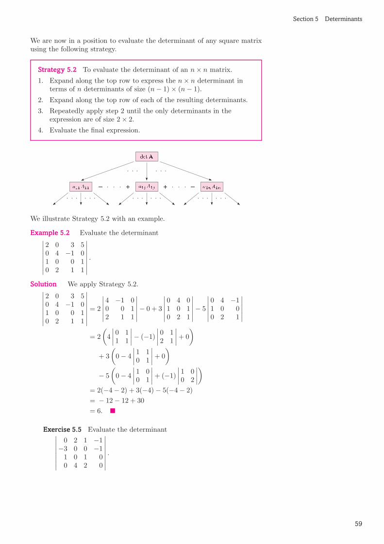
Section 5 Determinants
We are now in a position to evaluate the determinant of any square matrixusing the following strategy.
Strategy 5.2 To evaluate the determinant of an n× n matrix.
1. Expand along the top row to express the n× n determinant interms of n determinants of size (n− 1)× (n− 1).
2. Expand along the top row of each of the resulting determinants.
3. Repeatedly apply step 2 until the only determinants in theexpression are of size 2× 2.
4. Evaluate the final expression.
We illustrate Strategy 5.2 with an example.
Example 5.2 Evaluate the determinant∣
∣
∣
∣
∣
∣
∣
∣
2 0 3 50 4 −1 01 0 0 10 2 1 1
∣
∣
∣
∣
∣
∣
∣
∣
.
Solution We apply Strategy 5.2.∣
∣
∣
∣
∣
∣
∣
∣
2 0 3 50 4 −1 01 0 0 10 2 1 1
∣
∣
∣
∣
∣
∣
∣
∣
= 2
∣
∣
∣
∣
∣
∣
4 −1 00 0 12 1 1
∣
∣
∣
∣
∣
∣
− 0 + 3
∣
∣
∣
∣
∣
∣
0 4 01 0 10 2 1
∣
∣
∣
∣
∣
∣
− 5
∣
∣
∣
∣
∣
∣
0 4 −11 0 00 2 1
∣
∣
∣
∣
∣
∣
= 2
(
4
∣
∣
∣
∣
0 11 1
∣
∣
∣
∣
− (−1)
∣
∣
∣
∣
0 12 1
∣
∣
∣
∣
+ 0
)
+ 3
(
0− 4
∣
∣
∣
∣
1 10 1
∣
∣
∣
∣
+ 0
)
− 5
(
0− 4
∣
∣
∣
∣
1 00 1
∣
∣
∣
∣
+ (−1)
∣
∣
∣
∣
1 00 2
∣
∣
∣
∣
)
= 2(−4− 2) + 3(−4)− 5(−4− 2)
= − 12− 12 + 30
= 6.
Exercise 5.5 Evaluate the determinant∣
∣
∣
∣
∣
∣
∣
∣
0 2 1 −1−3 0 0 −11 0 1 00 4 2 0
∣
∣
∣
∣
∣
∣
∣
∣
.
59

Unit LA2 Linear equations and matrices
5.3 Properties of determinantsSuppose that A and B are two square matrices of the same size. Are thereany relationships between detA, detB, det(A+B) and det(AB)?
Exercise 5.6 Let A =
(
−3 12 −4
)
and B =
(
1 1−2 5
)
.
Evaluate detA, detB, det(A+B), det(AB) and (detA)(detB).Comment on your results.
You should have found in the solution to Exercise 5.6 that there does notappear to be a simple relationship for the addition of determinants; that is,we cannot easily express det(A+B) in terms of detA and detB.However, the identity
det(AB) = (detA)(detB)
holds for all square matrices A and B of the same size. The simplicity ofthis result is somewhat surprising, given the complexity of the definitionsof matrix multiplication and the determinant.
We collect together some results for determinants in the following theorem.
Theorem 5.1 Let A and B be two square matrices of the same size. We omit the proof.
Then the following hold:
(a) det(AB) = (detA)(detB);
(b) det I = 1;
(c) detAT = detA.
Elementary operations and determinants
Earlier, we saw that multiplication on the left by an elementary matrix has Theorem 4.8
the same effect as applying the associated elementary row operation. Here,we use elementary matrices to prove some useful results aboutdeterminants.
Exercise 5.7 Evaluate the following determinants, where k is any realnumber.
(a)
∣
∣
∣
∣
∣
∣
0 1 01 0 00 0 1
∣
∣
∣
∣
∣
∣
(b)
∣
∣
∣
∣
∣
∣
∣
∣
1 0 0 00 1 0 00 0 k 00 0 0 1
∣
∣
∣
∣
∣
∣
∣
∣
(c)
∣
∣
∣
∣
1 0k 1
∣
∣
∣
∣
The results of Exercise 5.7 are special cases of the following theorem.
Theorem 5.2 Let E be an elementary matrix, and let k be a We omit the proof.
non-zero real number.
(a) If E results from interchanging two rows of I, then detE = −1.
(b) If E results from multiplying a row of I by k, then detE = k.
(c) If E results from adding k times one row of I to another row,then detE = 1.
60

Section 5 Determinants
Zeros in a matrix greatly simplify the calculation of the determinant. If anentire row of the matrix is zero, then all the terms vanish and thedeterminant is zero. Other matrices with zero determinant are also easy torecognise.
Theorem 5.3 Let A be a square matrix. Then detA = 0 if any ofthe following hold:
(a) A has an entire row (or column) of zeros;
(b) A has two equal rows (or columns);
(c) A has two proportional rows (or columns). Two rows (or columns) of amatrix are proportional whenone is a multiple of the other.
Proof We prove the statements for rows. The results for columns follow,as Theorem 5.1(c) states that taking the transpose does not alter thedeterminant of a matrix.
(a) Each term in the expansion of the determinant of A contains oneentry from each row and each column of A. If an entire row of A iszero, then each term of the expansion contains at least one zero. Thedeterminant of A is therefore equal to zero.
(b) If the ith and jth rows of the matrix A are equal, then A remains thesame if these rows are interchanged. Let E be the elementary matrixobtained by interchanging the ith and jth rows of I. Then EA = A.Using Theorems 5.1 and 5.2, we have
detA = det(EA) = (detE)(detA) = −1× detA.
This implies that detA = 0, as required.
(c) Suppose that the ith row of A is equal to k times the jth row. Let Ebe the elementary matrix obtained from I by multiplying the ith rowby 1/k. Then the ith and jth rows of the matrix EA are equal. Thedeterminant of this matrix EA is zero, by (b) above. UsingTheorem 5.1, we have
(detE)(detA) = det(EA) = 0.
Now detE = 1/k, by Theorem 5.2. This implies that detA = 0, asrequired.
Exercise 5.8 Evaluate the determinant of the matrix
A =
1 −2 40 13 11
−2 4 −8
.
The evaluation of the determinant can be significantly simplified if a row ofthe matrix contains some zeros, as the following example illustrates.
Example 5.3 Evaluate the determinant of the matrix
A =
1 4 20 7 03 1 5
.
61

Unit LA2 Linear equations and matrices
Solution First notice that the second row of A has only one non-zeroentry. We interchange the top two rows of A, and apply Theorems 5.1and 5.2, giving
detA =
∣
∣
∣
∣
∣
∣
1 4 20 7 03 1 5
∣
∣
∣
∣
∣
∣
= (−1)
∣
∣
∣
∣
∣
∣
0 7 01 4 23 1 5
∣
∣
∣
∣
∣
∣
.
We use Strategy 5.2 to evaluate this determinant: The calculation has beensimplified by interchanging rows,as there is only one non-zeroterm in this expansion.
detA = (−1)
(
0− 7
∣
∣
∣
∣
1 23 5
∣
∣
∣
∣
+ 0
)
= 7((1 × 5)− (2× 3))
= −7.
Exercise 5.9 Evaluate the determinant of the matrix
A =
10 3 −4 20 2 0 10 6 0 0
−1 2 1 0
.
5.4 Determinants and inverses of matrices
Earlier, we stated that the inverse of a 2× 2 matrix A exists if and only ifdetA 6= 0. This extends to all square matrices.
Theorem 5.4 A square matrix A is invertible if and only ifdetA 6= 0.
Proof Let A be an n× n matrix.
We begin by assuming that A is invertible.
Since AA−1 = In, it follows from Theorem 5.1 that
(detA)(detA−1) = det(AA−1) = det In = 1.
Therefore neither detA nor detA−1 is 0.
We now assume that detA 6= 0. Let E1, . . . ,Ek be elementary matricessuch that Ek · · ·E2E1A = U is a matrix in row-reduced form. UsingTheorems 5.1 and 5.2 and the assumption that detA 6= 0, we have
detU = (detEk) · · · (detE2)(detE1)(detA) 6= 0.
Now this implies that U has no zero row, and therefore has a leading 1 ineach of its n rows. Hence U = In, and so, by the Invertibility Theorem,the matrix A is invertible, with
A−1 = Ek · · ·E2E1.
We saw in the proof of Theorem 5.4 above that if A is invertible, then(detA)(detA−1) = 1. This implies that
detA−1 =1
detA.
62
Section 5 Determinants
Until now, if we wanted to show that an n× n matrix A is invertible, wehad to produce an n× n matrix B such that
AB = I and BA = I.
The next theorem shows that if one of these conditions holds, then theother holds automatically. Thus, if we want to show that an n× n matrixA is invertible, it is enough to produce an n× n matrix B satisfying either
condition.
Theorem 5.5 Let A and B be square matrices of the same size.Then AB = I if and only if BA = I.
Proof We first assume that AB = I. Then by Theorem 5.1,
(detA)(detB) = det(AB) = det I = 1.
This implies that
detA 6= 0 and detB 6= 0,
so, by Theorem 5.4, A and B are both invertible.
Now,
A−1 = A−1I,
and we can write I as AB, so
A−1 = A−1(AB) = (A−1A)B = IB = B,
and therefore
BA = A−1A = I,
as required.
The same argument, with the roles of A and B interchanged, proves theconverse.
We summarise the results on the invertibility of a matrix A as follows.
Theorem 5.6 Summary Theorem
Let A be an n× n matrix. Then the following statements are This collects togetherTheorems 4.5, 4.7 and 5.4.equivalent.
(a) A is invertible.
(b) detA 6= 0.
(c) The row-reduced form of A is In.
(d) The system Ax = b has precisely one solution for each n× 1matrix b.
(e) The system Ax = 0 has only the trivial solution.
To conclude this section, we collect together some of the most importantproperties of matrices that we have met in this unit.
63

Unit LA2 Linear equations and matrices
Summary of properties of matrices
Let A and B be two square matrices of the same size. Then
det(AB) = (detA)(detB),
(AB)T = BTAT ,
detAT = detA.
If A and B are invertible, then
(AB)−1 = B−1A−1,
detA−1 =1
detA.
Further exercises
Exercise 5.10 Let A =
(
2 04 1
)
and B =
(
1 −1−2 5
)
. Evaluate the
following.
(a) detA (b) detB (c) det(A+B)
(d) det(AB) (e) det(BA) (f) det(A2)
(g) detAT (h) det(AB)T (i) detA−1
Exercise 5.11 Determine whether or not each of the following matrices isinvertible, and find the inverse where it exists.
(a)
(
2 11 2
)
(b)
(
2 −2−1 1
)
(c)
(
10 21−4 −7
)
Exercise 5.12 Evaluate the determinant of each of the following matrices.
(a)
5 −31 10 12−1 4 −2 42 10 4 163 17 6 21
(b)
7 10 −1 0 21 5 0 2 00 2 0 0 03 −6 3 7 13 4 3 0 1
Exercise 5.13 Determine whether or not each of the following matrices isinvertible.
(a)
2 1 41 −1 3
−2 1 5
(b)
1 2 12 1 22 2 2
(c)
1 0 0 02 1 0 03 2 1 04 3 2 1
Exercise 5.14 Prove that an n× n matrix A is invertible if and only ifAAT is invertible.
64

Section 6 Summary

Unit LA2 Linear equations and matrices
Solutions to the exercises
1.1 (a) This is a linear equation.
(b) This is not a linear equation. The third terminvolves the product of x3 and x4.
(c) This is a linear equation.
(d) This is not a linear equation. For example, thesecond term, a2x
22, involves a product of unknowns.
1.2 A general homogeneous system of m linearequations in n unknowns is
a11x1 + · · · + a1nxn = 0,a21x1 + · · · + a2nxn = 0,...
......
am1x1 + · · · + amnxn = 0.
We substitute the values x1 = 0, x2 = 0, . . . , xn = 0into the equations of the system:
a110 + · · · + a1n0 = 0,a210 + · · · + a2n0 = 0,...
......
am10 + · · · + amn0 = 0.
All the equations are satisfied, whatever the values ofthe coefficients aij . The solution set thereforecontains the trivial solution
x1 = 0, x2 = 0, . . . , xn = 0.
1.3 We label the equations of the system,
r1r2
{
x + y = 4,2x − y = 5,
and apply elementary operations to simplify thesystem.
First we eliminate the unknown x from the secondequation:
r2 → r2 − 2r1
{
x + y = 4,− 3y = −3.
We then simplify this equation,
r2 → −1
3r2
{
x + y = 4,y = 1,
before using it to eliminate the unknown y from thefirst equation of the system:
r1 → r1 − r2{
x = 3,y = 1.
We conclude that there is a unique solution—namely,
x = 3, y = 1.
1.4 We label the equations of the system,
r1r2r3
x + y − z = 8,2x − y + z = 1,−x + 3y + 2z = −8,
and apply elementary operations to simplify thesystem.
First we use the r1 equation to eliminate theunknown x from the other equations:
r2 → r2 − 2r1r3 → r3 + r1
x + y − z = 8,− 3y + 3z = −15,
4y + z = 0.
We now simplify r2,
r2 → −1
3r2
x + y − z = 8,y − z = 5,
4y + z = 0,
and use it to eliminate the y-terms from r1 and r3:
r1 → r1 − r2
r3 → r3 − 4r2
x = 3,y − z = 5,
5z = −20.
We now simplify r3,
r3 → 1
5r3
x = 3,y − z = 5,
z = −4,
and use it to eliminate the z-term from r2:
r2 → r2 + r3
x = 3,y = 1,
z = −4.
We conclude that there is a unique solution—namely,
x = 3, y = 1, z = −4.
1.5 We label the equations of the system, and applyelementary operations to simplify the system.
r1r2r3
x + 3y − z = 4−x + 2y − 4z = 6x + 2y = 2
r2 → r2 + r1r3 → r3 − r1
x + 3y − z = 45y − 5z = 10
− y + z = −2
r2 → 1
5r2
x + 3y − z = 4y − z = 2
− y + z = −2
r1 → r1 − 3r2
r3 → r3 + r2
x + 2z = −2y − z = 2
0 = 0
The r3 equation (0 = 0) gives no constraints on x, yand z. We cannot simplify the system further, andconclude that there are infinitely many solutions. Asboth remaining equations involve a z-term, we set zequal to the real parameter k, and write the generalsolution as
x = −2− 2k, y = 2 + k, z = k, k ∈ R.
66

Solutions to the exercises
1.6 We label the equations of the system, and applyelementary operations to simplify the system.
r1r2r3
x + y + z = 6−x + y − 3z = −22x + y + 3z = 6
r2 → r2 + r1r3 → r3 − 2r1
x + y + z = 62y − 2z = 4
− y + z = −6
r2 → 1
2r2
x + y + z = 6y − z = 2
− y + z = −6
r1 → r1 − r2
r3 → r3 + r2
x + 2z = 4y − z = 2
0 = −4
The r3 equation is 0 = −4, so we conclude that thesolution set is empty—the system is inconsistent.
(We have chosen to use elementary operations tosolve the systems of equations in the further exerciseson Section 1. If you have been using the furtherexercises for revision, you may have preferred to usethe methods of Section 2. Of course, you shouldobtain the same answers by either method.)
1.7 (a) We label the equations, and applyelementary operations to simplify the system.
r1r2r3
x + 4y = −72x − y = 4−x + 2y = −5
r2 → r2 − 2r1r3 → r3 + r1
x + 4y = −7− 9y = 18
6y = −12
r2 → −1
9r2
x + 4y = −7y = −2
6y = −12
r1 → r1 − 4r2
r3 → r3 − 6r2
x = 1y = −20 = 0
We conclude that there is a unique solution—namely,x = 1, y = −2.
(b) We label the equations, and apply elementaryoperations to simplify the system.
r1r2
{
4x − 6y = −2−6x + 9y = −3
r1 → 1
4r1
{
x − 3
2y = −1
2
−6x + 9y = −3
r2 → r2 +6r1
{
x − 3
2y = −1
2
0 = −6
The r2 equation is 0 = −6, so we conclude that thesolution set is empty—the system is inconsistent.
(c) We label the equations, and apply elementaryoperations to simplify the system.
r1r2r3
p + q + r = 5p + 2q + 3r = 11
3p + q + 4r = 13
r2 → r2 − r1r3 → r3 − 3r1
p + q + r = 5q + 2r = 6
− 2q + r = −2
r1 → r1 − r2
r3 → r3 +2r2
p − r = −1q + 2r = 6
5r = 10
r3 → 1
5r3
p − r = −1q + 2r = 6
r = 2
r1 → r1 + r3r2 → r2 − 2r3
p = 1q = 2
r = 2
We conclude that there is a unique solution—namely,p = 1, q = 2, r = 2.
1.8 The points of intersection of the three planescorrespond to the solutions of the followinghomogeneous system of linear equations in the threeunknowns x, y and z:
x + y − z = 0,y − 2z = 0,
3x − y + 5z = 0.
We label the equations, and apply elementaryoperations to simplify the system.
r1r2r3
x + y − z = 0y − 2z = 0
3x − y + 5z = 0
r3 → r3 − 3r1
x + y − z = 0y − 2z = 0
− 4y + 8z = 0
r1 → r1 − r2
r3 → r3 +4r2
x + z = 0y − 2z = 0
0 = 0
The r3 equation (0 = 0) gives no constraints on x, yand z. We cannot simplify the system further, andconclude that there are infinitely many solutions.
As both equations involve a z-term, we set z equal tothe real parameter k, giving
x = −k, y = 2k, z = k, k ∈ R.
The three planes intersect in a line.
67

Unit LA2 Linear equations and matrices
1.9 We label the equations, and apply elementaryoperations to simplify the system.
r1r2r3r4
a − b − 2c + d = 3b + c + d = 3
a − b − c + 2d = 7b + c + 2d = 7
r3 → r3 − r1
a − b − 2c + d = 3b + c + d = 3
c + d = 4b + c + 2d = 7
r1 → r1 + r2
r4 → r4 − r2
a − c + 2d = 6b + c + d = 3
c + d = 4d = 4
r1 → r1 + r3r2 → r2 − r3
a + 3d = 10b = −1
c + d = 4d = 4
r1 → r1 − 3r4
r3 → r3 − r4
a = −2b = −1
c = 0d = 4
We conclude that there is a unique solution—namely,a = −2, b = −1, c = 0, d = 4.
2.1 (a) The augmented matrix of the system is
4 −2 0 −70 1 3 00 −3 1 3
.
(b) The corresponding system is
2x + 3y + 7w = 1,y − 7z = −1,
x + 3z − w = 2.
2.2 (a) Not row-reduced; it has neither property 1nor property 2.
(b) Not row-reduced; it does not have property 3.
(c) Row-reduced.
(d) Row-reduced.
(e) Not row-reduced; it does not have property 4.
2.3 (a) The augmented matrix corresponds to thesystem{
x1 = 1
3,
x2 = 2
3.
The solution is x1 = 1
3, x2 =
2
3.
(b) The augmented matrix corresponds to thesystem
x1 + 6x3 = 0,x2 + 7x3 = 0,
0 = 1.
The third equation cannot be satisfied, so there areno solutions.
(c) The augmented matrix corresponds to thesystem
x1 + 3x2 + 2x4 = −7,x3 − 3x4 = 8,
x5 = 11,
that is,
x1 = −7 − 3x2 − 2x4,x3 = 8 + 3x4,x5 = 11.
Setting x2 = k and x4 = l (k, l ∈ R), we obtain thegeneral solution
x1 = −7− 3k − 2l,
x2 = k,
x3 = 8 + 3l,
x4 = l,
x5 = 11.
(d) The augmented matrix corresponds to thesystem
x1 + x4 = 0,x2 + 4x4 = 3,
x3 = 0,
that is,
x1 = − x4,x2 = 3 − 4x4,x3 = 0.
Setting x4 = k (k ∈ R), we obtain the generalsolution
x1 = −k,
x2 = 3− 4k,
x3 = 0,
x4 = k.
2.4 (a) We follow Strategy 2.1 in Frame 10.
If you followed Strategy 2.1, then your sequence ofrow operations should be the same as ours.
r1r2r3r4
1 5 1 4 5 −11 5 3 12 11 33 15 −1 −4 3 −6
−2 −10 1 2 −7 6
r2 → r2 − r1r3 → r3 − 3r1r4 → r4 +2r1
1 5 1 4 5 −10 0 2 8 6 40 0 −4 −16 −12 −30 0 3 10 3 4
r2 → 1
2r2
1 5 1 4 5 −10 0 1 4 3 20 0 −4 −16 −12 −30 0 3 10 3 4
r1 → r1 − r2
r3 → r3 +4r2r4 → r4 − 3r2
1 5 0 0 2 −30 0 1 4 3 20 0 0 0 0 50 0 0 −2 −6 −2
68

Solutions to the exercises
r3 ↔ r4
1 5 0 0 2 −30 0 1 4 3 20 0 0 −2 −6 −20 0 0 0 0 5
r3 → −1
2r3
1 5 0 0 2 −30 0 1 4 3 20 0 0 1 3 10 0 0 0 0 5
r2 → r2 − 4r3
1 5 0 0 2 −30 0 1 0 −9 −20 0 0 1 3 10 0 0 0 0 5
r4 → 1
5r4
1 5 0 0 2 −30 0 1 0 −9 −20 0 0 1 3 10 0 0 0 0 1
r1 → r1 +3r4r2 → r2 +2r4r3 → r3 − r4
1 5 0 0 2 00 0 1 0 −9 00 0 0 1 3 00 0 0 0 0 1
This is the row-reduced form of the matrix.
(b) We follow Strategy 2.1 in Frame 10.
The sequence of row operations that we have used toreduce this matrix to row-reduced form might bedifferent from the sequence that you used in followingStrategy 2.1, since in the first step shown below(which corresponds to step 2 of the strategy) wechose to interchange row 1 with row 5, while youmight have chosen to interchange row 1 with anotherrow. However, your final row-reduced matrix shouldbe the same as ours, since, by Theorem 2.1 inFrame 16, the row-reduced form of a matrix isunique.
r1r2r3r4r5
0 −8 8 −14−1 0 −4 −6−1 8 −12 82 8 0 241 4 0 14
r1 ↔ r5
1 4 0 14−1 0 −4 −6−1 8 −12 82 8 0 240 −8 8 −14
r2 → r2 + r1r3 → r3 + r1r4 → r4 − 2r1
1 4 0 140 4 −4 80 12 −12 220 0 0 −40 −8 8 −14
r2 → 1
4r2
1 4 0 140 1 −1 20 12 −12 220 0 0 −40 −8 8 −14
r1 → r1 − 4r2
r3 → r3 − 12r2
r5 → r5 + 8r2
1 0 4 60 1 −1 20 0 0 −20 0 0 −40 0 0 2
r3 → −1
2r3
1 0 4 60 1 −1 20 0 0 10 0 0 −40 0 0 2
r1 → r1 − 6r3r2 → r2 − 2r3
r4 → r4 + 4r3r5 → r5 − 2r3
1 0 4 00 1 −1 00 0 0 10 0 0 00 0 0 0
This is the row-reduced form of the matrix.
2.5 In each of the following, the sequence of rowoperations that you used to reduce the matrix maydiffer from the sequence that we use, but you shouldobtain the same final answer.
(a) We follow Strategy 2.2 in Frame 17, androw-reduce the augmented matrix.
r1r2r3
3 5 −12 41 1 0 22 3 −4 5
r1 ↔ r2
1 1 0 23 5 −12 42 3 −4 5
(We have chosen to perform the row operationr1 ↔ r2 instead of r1 → 1
3r1, to avoid creating
awkward fractions.)
r2 → r2 − 3r1r3 → r3 − 2r1
1 1 0 20 2 −12 −20 1 −4 1
r2 → 1
2r2
1 1 0 20 1 −6 −10 1 −4 1
r1 → r1 − r2
r3 → r3 − r2
1 0 6 30 1 −6 −10 0 2 2
r3 → 1
2r3
1 0 6 30 1 −6 −10 0 1 1
r1 → r1 − 6r3r2 → r2 +6r3
1 0 0 −30 1 0 50 0 1 1
This matrix is in row-reduced form.
69

Unit LA2 Linear equations and matrices
The corresponding system is
x = −3,y = 5,
z = 1.
Thus the solution is x = −3, y = 5, z = 1.
(b) We follow Strategy 2.2 in Frame 17, androw-reduce the augmented matrix.
r1r2r3
1 −4 −4 3 6 22 −5 −6 6 9 32 4 0 9 2 0
r2 → r2 − 2r1r3 → r3 − 2r1
1 −4 −4 3 6 2
0 3 2 0 −3 −1
0 12 8 3 −10 −4
r2 → 1
3r2
1 −4 −4 3 6 2
0 1 2
30 −1 −1
3
0 12 8 3 −10 −4
(Note that here we cannot find a row operation thatcould be performed instead of r2 → 1
3r2 to create a
leading 1 while avoiding fractions. Fractions areunavoidable.)
r1 → r1 + 4r2
r3 → r3 − 12r2
1 0 −4
33 2 2
3
0 1 2
30 −1 −1
3
0 0 0 3 2 0
r3 → 1
3r3
1 0 −4
33 2 2
3
0 1 2
30 −1 −1
3
0 0 0 1 2
30
r1 → r1 − 3r3
1 0 −4
30 0 2
3
0 1 2
30 −1 −1
3
0 0 0 1 2
30
This matrix is in row-reduced form.The corresponding system is
x1 − 4
3x3 = 2
3,
x2 + 2
3x3 − x5 = −1
3,
x4 + 2
3x5 = 0,
that is,
x1 = 2
3+ 4
3x3,
x2 = −1
3− 2
3x3 + x5,
x4 = − 2
3x5.
Setting x3 = k and x5 = l (k, l ∈ R), we obtain thegeneral solution
x1 = 2
3+ 4
3k,
x2 = −1
3− 2
3k + l,
x3 = k,
x4 = −2
3l,
x5 = l.
2.6 (a) Not row-reduced; it does not haveproperty 3.
(b) Row-reduced.
(c) Row-reduced.
(d) Not row-reduced; it does not have property 4.
(e) Row-reduced.
(f) Row-reduced.
2.7 (a) The augmented matrix corresponds to thesystem
x1 = 7,x2 = −6,
x3 = 5.
The solution is x1 = 7, x2 = −6, x3 = 5.
(b) The augmented matrix corresponds to thesystem{
x1 + 1
7x2 = 1,
x3 = 3,
that is,{
x1 = 1 − 1
7x2,
x3 = 3.
Setting x2 = k (k ∈ R), we obtain the generalsolution
x1 = 1− 1
7k,
x2 = k,
x3 = 3.
(c) The augmented matrix corresponds to thesystem
x1 + 4x3 = 0,x2 − 3x3 = 0,
x4 = 0,
that is,
x1 = −4x3,x2 = 3x3,x4 = 0.
Setting x3 = k (k ∈ R), we obtain the generalsolution
x1 = −4k,
x2 = 3k,
x3 = k,
x4 = 0.
(d) The augmented matrix corresponds to thesystem
x1 + 3x2 − 2x4 = 0,x3 + 2x4 + x5 = 0,
0 = 1.
The third equation cannot be satisfied, so there areno solutions.
70
Solutions to the exercises
(e) The augmented matrix corresponds to thesystem{
x1 − 5x3 = 4,x2 − 7x3 + 3x4 = 12,
that is,{
x1 = 4 + 5x3,x2 = 12 + 7x3 − 3x4.
Setting x3 = k and x4 = l (k, l ∈ R), we obtain thegeneral solution
x1 = 4 + 5k,
x2 = 12 + 7k − 3l,
x3 = k,
x4 = l.
2.8 We follow Strategy 2.2 in Frame 17.
(a) We row-reduce the augmented matrix.
r1r2r3r4
3 −11 −3 32 −6 −2 15 −17 −6 24 −8 0 7
r1 → r1 − r2
1 −5 −1 22 −6 −2 15 −17 −6 24 −8 0 7
r2 → r2 − 2r1r3 → r3 − 5r1r4 → r4 − 4r1
1 −5 −1 20 4 0 −30 8 −1 −80 12 4 −1
r2 → 1
4r2
1 −5 −1 2
0 1 0 −3
4
0 8 −1 −8
0 12 4 −1
r1 → r1 + 5r2
r3 → r3 − 8r2
r4 → r4 − 12r2
1 0 −1 −7
4
0 1 0 −3
4
0 0 −1 −2
0 0 4 8
r3 → −r3
1 0 −1 −7
4
0 1 0 −3
4
0 0 1 2
0 0 4 8
r1 → r1 + r3
r4 → r4 − 4r3
1 0 0 1
4
0 1 0 −3
4
0 0 1 2
0 0 0 0
This matrix is in row-reduced form.
The corresponding system is
x = 1
4,
y = −3
4,
z = 2.
Thus the solution is x = 1
4, y = −3
4, z = 2.
(b) We row-reduce the augmented matrix.
r1r2r3r4
1 0 −4 −2 −11 2 −2 4 62 4 −3 9 92 1 −5 1 −4
r2 → r2 − r1r3 → r3 − 2r1r4 → r4 − 2r1
1 0 −4 −2 −10 2 2 6 70 4 5 13 110 1 3 5 −2
r2 → r2 − r4
1 0 −4 −2 −10 1 −1 1 90 4 5 13 110 1 3 5 −2
r3 → r3 − 4r2r4 → r4 − r2
1 0 −4 −2 −10 1 −1 1 90 0 9 9 −250 0 4 4 −11
r3 → r3 − 2r4
1 0 −4 −2 −10 1 −1 1 90 0 1 1 −30 0 4 4 −11
r1 → r1 +4r3r2 → r2 + r3
r4 → r4 − 4r3
1 0 0 2 −130 1 0 2 60 0 1 1 −30 0 0 0 1
This matrix is in row-reduced form.The corresponding system is
a + 2d = −13,b + 2d = 6,
c + d = −3,0 = 1.
The fourth equation cannot be satisfied, so there areno solutions.
The last matrix in the above row-reductioncorresponds to a system containing the equation0 = 1. We could have concluded that the givensystem has no solutions at this point.
71

Unit LA2 Linear equations and matrices
(c) We row-reduce the augmented matrix.
r1r2r3r4
2 2 −5 6 10 −22 2 −6 6 8 02 0 −1 2 7 71 2 −5 5 4 −3
r1 ↔ r4
1 2 −5 5 4 −32 2 −6 6 8 02 0 −1 2 7 72 2 −5 6 10 −2
r2 → r2 − 2r1r3 → r3 − 2r1r4 → r4 − 2r1
1 2 −5 5 4 −30 −2 4 −4 0 60 −4 9 −8 −1 130 −2 5 −4 2 4
r2 → −1
2r2
1 2 −5 5 4 −30 1 −2 2 0 −30 −4 9 −8 −1 130 −2 5 −4 2 4
r1 → r1 − 2r2
r3 → r3 +4r2r4 → r4 +2r2
1 0 −1 1 4 30 1 −2 2 0 −30 0 1 0 −1 10 0 1 0 2 −2
r1 → r1 + r3r2 → r2 +2r3
r4 → r4 − r3
1 0 0 1 3 40 1 0 2 −2 −10 0 1 0 −1 10 0 0 0 3 −3
r4 → 1
3r4
1 0 0 1 3 40 1 0 2 −2 −10 0 1 0 −1 10 0 0 0 1 −1
r1 → r1 − 3r4r2 → r2 +2r4r3 → r3 + r4
1 0 0 1 0 70 1 0 2 0 −30 0 1 0 0 00 0 0 0 1 −1
This matrix is in row-reduced form.The corresponding system is
x1 + x4 = 7,x2 + 2x4 = −3,
x3 = 0,x5 = −1,
that is,
x1 = 7 − x4,x2 = −3 − 2x4,x3 = 0,x5 = −1.
Setting x4 = k (k ∈ R), we obtain the generalsolution
x1 = 7− k,
x2 = −3− 2k,
x3 = 0,
x4 = k,
x5 = −1.
3.1 (a) This is a 2× 4 matrix, so it is not square.The (2, 3)-entry is 5.
(b) This is a 3× 3 matrix, so it is square.The (2, 3)-entry is 0.
(c) This is a 2× 2 matrix, so it is square.There is no (2, 3)-entry.
3.2 We add corresponding entries.
(a)(
1 −3−2 54
)
+
(
2 04 1
)
=
(
3 −32 55
)
(b)(
2 04 1
)
+
(
1 −3−2 54
)
=
(
3 −32 55
)
(c) This sum cannot be evaluated, since thematrices are of different sizes.
(d)
0 6 −21 8 20 3 4
+
1 2 91 0 43 −4 1
=
1 8 72 8 63 −1 5
3.3 We add corresponding entries of the threematrices A = (aij), B = (bij) and C = (cij). The(i, j)-entry of the matrix A+ (B+C) isaij + (bij + cij), and that of (A+B) +C is(aij + bij) + cij. Now, aij , bij and cij are scalars, andscalar addition is associative, soaij + (bij + cij) = (aij + bij) + cij. Therefore
A+ (B+C) = (A+B) +C.
3.4 We add corresponding entries of the twomatrices. The (i, j)-entry of the matrix A+ 0 isaij + 0 = aij. Therefore
A+ 0 = A.
3.5 (a) This difference cannot be evaluated, sincethe matrices are of different sizes.
(b)(
5 8 127 2 −1
)
−
(
3 10 24 9 21
)
=
(
2 −2 103 −7 −22
)
3.6 (a) 4A = 4
5 −32 3
−1 0
=
20 −128 12
−4 0
(b) 4B = 4
2 1−2 −73 5
=
8 4−8 −2812 20
4A+ 4B =
20 −128 12
−4 0
+
8 4−8 −2812 20
(c)
=
28 −80 −168 20
72

Solutions to the exercises
A+B =
5 −32 3
−1 0
+
2 1−2 −73 5
(d)
=
7 −20 −42 5
,
thus
4(A+B) =
28 −80 −168 20
.
3.7 To obtain the (2, 1)-entry of the product AB,we take the dot product of the second row of A withthe first column of B. The (2, 1)-entry of AB is
(4, 5, 6) . (1, 4, 7) = (4× 1) + (5× 4) + (6× 7)
= 4 + 20 + 42
= 66.
3.8 (a) The product of a 3× 2 matrix with a 2× 1matrix is a 3× 1 matrix:
2 −10 31 2
(
32
)
=
467
.
(b) The product of a 1× 2 matrix with a 2× 2matrix is a 1× 2 matrix:(
2 1)
(
1 60 2
)
=(
2 14)
.
(c) This product cannot be formed, since the firstmatrix has 1 column and the second has 2 rows.
(d) The product of a 2× 1 matrix with a 1× 3matrix is a 2× 3 matrix:(
12
)
(
3 0 −4)
=
(
3 0 −46 0 −8
)
.
(e) The product of a 2× 3 matrix with a 3× 3matrix is a 2× 3 matrix:(
3 1 20 5 1
)
−2 0 11 3 04 1 −1
=
(
3 5 19 16 −1
)
.
3.9 The product of a 2× 2 matrix with a 2× 2matrix is a 2× 2 matrix. The products AB and BA
are therefore both 2× 2 matrices:
AB =
(
1 13 2
)(
1 42 1
)
=
(
3 57 14
)
,
BA =
(
1 42 1
)(
1 13 2
)
=
(
13 95 4
)
.
The products AB and BA are not the same.
Matrix multiplication is therefore not commutative.
3.10 The product of a 2× 2 matrix with a 2× 2matrix is a 2× 2 matrix.
(a) AB =
(
1 00 7
)(
−3 00 4
)
=
(
−3 00 28
)
(b) BA =
(
−3 00 4
)(
1 00 7
)
=
(
−3 00 28
)
Note that AB and BA are equal in this case.
(c) Matrix multiplication is associative, so
ABC = (AB)C = A(BC)
=
((
1 00 7
)(
−3 00 4
))(
2 00 12
)
=
(
−3 00 28
)(
2 00 12
)
=
(
−6 00 336
)
.
3.11 (a) The matrix
1 1 10 2 20 0 3
is
upper-triangular.
(b) The matrix
(
9 00 0
)
is diagonal,
upper-triangular and lower-triangular.
(c) The matrix
0 0 10 1 21 2 3
is not diagonal,
upper-triangular or lower-triangular.
(d) The matrix
(
1 01 0
)
is lower-triangular.
3.12 (a) The transpose of a 3× 2 matrix is a 2× 3matrix:
1 40 2
−6 10
T
=
(
1 0 −64 2 10
)
.
(b) The transpose of a 3× 3 matrix is a 3× 3matrix:
2 1 20 3 −54 7 0
T
=
2 0 41 3 72 −5 0
.
(c) The transpose of a 1× 3 matrix is a 3× 1matrix:
(
10 4 6)T
=
1046
.
(d) The transpose of a 2× 2 matrix is a 2× 2matrix:(
1 00 2
)T
=
(
1 00 2
)
.
In fact, AT = A for all diagonal matrices.
3.13 (a) Here,
AT =
(
1 3 52 4 6
)
,
BT =
(
7 9 118 10 12
)
73

Unit LA2 Linear equations and matrices
and
A+B =
8 1012 1416 18
.
So
(A+B)T =
(
8 12 1610 14 18
)
and
AT +BT =
(
1 3 52 4 6
)
+
(
7 9 118 10 12
)
=
(
8 12 1610 14 18
)
= (A+B)T .
(b) Here,
CT =
(
1 10 1
)
and
AC =
1 23 45 6
(
1 01 1
)
=
3 27 4
11 6
.
So
(AC)T =
(
3 7 112 4 6
)
.
The product ATCT cannot be formed, since AT is a2× 3 matrix and CT is a 2× 2 matrix.The product CTAT does, however, exist:
CTAT =
(
1 10 1
)(
1 3 52 4 6
)
=
(
3 7 112 4 6
)
= (AC)T .
3.14 (a) A+B =
(
3 33 3
)
(b) A−B =
(
−1 93 −11
)
(c) B−A = −(A−B) =
(
1 −9−3 11
)
(d) AB =
(
2 396 −37
)
(e) BA =
(
−7 2421 −28
)
(f) A2 =
(
19 −18−9 34
)
(g) AT =
(
1 36 −4
)
(h) BT =
(
2 0−3 7
)
(i) ATBT = (BA)T =
(
−7 2124 −28
)
3.15 (a) FB : 3× 3, E : 3× 3.
The matrix FB+E exists and is 3× 3.
(b) FT : 4× 3, GFT : 2× 3, AD : 2× 4,ADB : 2× 3.
The matrix GFT −ADB exists and is 2× 3.
(c) BF : 4× 4, FB : 3× 3, (FB)T : 3× 3.
The matrix BF− (FB)T does not exist, since BF
and (FB)T are different sizes.
(d) AD : 2× 4, AD+G : 2× 4, C : 3× 2.
The matrix C(AD+G) exists and is 3× 4.
(e) CA : 3× 1, (CA)T : 1× 3, D : 1× 4.
The matrix (CA)TD does not exist, since (CA)T issize 1× 3 and D is size 1× 4.
(f) ETBTGTCT = (CGBE)T .
CG : 3× 4, CGB : 3× 3, CGBE : 3× 3,(CGBE)T : 3× 3.
The matrix ETBTGTCT exists and is 3× 3.
3.16 Let A = (aij) and B = (bij) be matrices of thesame size. Then the (i, j)-entry of k(A+B) isk(aij + bij).
Now, kA = (kaij) and kB = (kbij), so the (i, j)-entryof kA+ kB is kaij + kbij = k(aij + bij).
The (i, j)-entries of k(A+B) and kA+ kB areequal. Thus
k(A+B) = kA+ kB.
3.17 The (i, j)-entry of the product ImA is obtainedby taking the dot product of the ith row of Im withthe jth column of A. Now, the ith row of Im has a 1in the ith position and 0s elsewhere. Therefore thedot product will give the ith entry of the jth columnof A, that is, the (i, j)-entry of A. Thus ImA = A.
The (i, j)-entry of the product AIn is obtained bytaking the dot product of the ith row of A with thejth column of In. Now, the jth column of In has a 1in the jth position and 0s elsewhere. Therefore thedot product will give the jth entry of the ith rowof A, that is, the (i, j)-entry of A. Thus AIn = A.
4.1 Suppose, for a contradiction, that there exists a
matrix B =
(
a bc d
)
such that AB = I, that is,
(
1 −1−1 1
)(
a bc d
)
=
(
1 00 1
)
.
Multiplying out the matrices on the left-hand side:(
a− c b− d−a+ c −b+ d
)
=
(
1 00 1
)
.
Looking at the entries in the first column, we musthave a− c = 1 and −a+ c = 0, that is, a− c = 1 anda− c = 0. This contradiction shows that there existsno such matrix B. (A similar conclusion arises fromlooking at the entries in the second column.)
74

Solutions to the exercises
4.2 The equation II = I shows that I is invertible,with inverse I.
4.3 To prove that AB is invertible, with inverseB−1A−1, we have to show that
(AB)(B−1A−1) = I and (B−1A−1)(AB) = I.
But, by associativity,
(AB)(B−1A−1) = A(BB−1)A−1
= AIA−1
= AA−1 = I,
and, similarly,
(B−1A−1)(AB) = B−1(A−1A)B
= B−1IB
= B−1B = I.
The required result follows.
4.4 (a) We row-reduce (A | I).
r1r2
(
2 4 1 04 1 0 1
)
r1 → 1
2r1
(
1 2 1
20
4 1 0 1
)
r2 → r2 − 4r1
(
1 2 1
20
0 −7 −2 1
)
r2 → −1
7r2
(
1 2 1
20
0 1 2
7−1
7
)
r1 → r1 − 2r2(
1 0 − 1
14
2
7
0 1 2
7−1
7
)
The left half has been reduced to I, so the givenmatrix is invertible; its inverse is(
− 1
14
2
7
2
7−1
7
)
.
(b) We row-reduce (A | I).
r1r2r3
1 1 −4 1 0 02 1 −6 0 1 0
−3 −1 9 0 0 1
r2 → r2 − 2r1r3 → r3 +3r1
1 1 −4 1 0 00 −1 2 −2 1 00 2 −3 3 0 1
r2 → −r2
1 1 −4 1 0 00 1 −2 2 −1 00 2 −3 3 0 1
r1 → r1 − r2
r3 → r3 − 2r2
1 0 −2 −1 1 00 1 −2 2 −1 00 0 1 −1 2 1
r1 → r1 +2r3r2 → r2 +2r3
1 0 0 −3 5 20 1 0 0 3 20 0 1 −1 2 1
The left half has been reduced to I, so the givenmatrix is invertible; its inverse is
−3 5 20 3 2
−1 2 1
.
(c) We row-reduce (A | I).
r1
r2
r3
2 4 6 1 0 0
1 2 4 0 1 0
5 10 5 0 0 1
r1 → 1
2r1
1 2 3 1
20 0
1 2 4 0 1 0
5 10 5 0 0 1
r2 → r2 − r1
r3 → r3 − 5r1
1 2 3 1
20 0
0 0 1 −1
21 0
0 0 −10 −5
20 1
The usual strategy for row-reduction has created aleading 1 in the second row that does not lie on theleading diagonal of the left half. Hence the left halfcannot reduce to I, and therefore the given matrix isnot invertible.
4.5 The matrix form of the system is
1 1 2−1 0 −43 2 10
xyz
=
12
−1
.
Multiplying this equation on the left by the inverse ofthe coefficient matrix gives the solution
xyz
=
4 −3 −2−1 2 1−1 1
2
1
2
12
−1
=
02
−1
2
;
that is, x = 0, y = 2, z = −1
2.
4.6
(a)
(
5 00 1
) (
1 2 33 2 1
)
=
(
5 10 153 2 1
)
elementary A matrixmatrix obtained when
associated with r1 → 5r1r1 → 5r1 is performed on A
(b)
1 0 0 00 1 0 30 0 1 00 0 0 1
1 23 45 67 8
=
1 224 285 67 8
elementary B matrixmatrix obtained when
associated with r2 → r2 + 3r4r2 → r2 + 3r4 is performed on B
75
Unit LA2 Linear equations and matrices
4.7 (a) The inverse elementary row operation ofr1 → r1 − 2r2 is r1 → r1 + 2r2.
The working below shows the sequence of two rowoperations performed on the given matrix.
r1r2
(
1 2 34 5 6
)
r1 → r1 − 2r2(
−7 −8 −94 5 6
)
r1 → r1 +2r2(
1 2 34 5 6
)
(b) The inverse elementary row operation ofr1 ↔ r2 is r1 ↔ r2.
The working below shows the sequence of two rowoperations performed on the given matrix.
r1r2
(
1 2 34 5 6
)
r1 ↔ r2(
4 5 61 2 3
)
r1 ↔ r2(
1 2 34 5 6
)
(c) The inverse elementary row operation ofr2 → −3r2 is r2 → −1
3r2.
The working below shows the sequence of two rowoperations performed on the given matrix.
r1r2
(
1 2 34 5 6
)
r2 → −3r2
(
1 2 3−12 −15 −18
)
r2 → −1
3r2
(
1 2 34 5 6
)
4.8 The given matrix has associated elementary rowoperation r1 → 2r1, which has inverse r1 → 1
2r1. The
inverse of the given matrix is the elementary matrixassociated with this inverse row operation, which is
1
20 0
0 1 0
0 0 1
.
4.9 To prove that kA is invertible, with inverse(1/k)A−1, we have to show that
(kA)
(
1
kA−1
)
= I and
(
1
kA−1
)
(kA) = I.
But
(kA)
(
1
kA−1
)
=
(
k ×1
k
)
(AA−1) = 1I = I,
and(
1
kA−1
)
(kA) =
(
1
k× k
)
(A−1A) = 1I = I,
as required.
4.10 (a) We row-reduce (A | I).
r1r2
(
2 3 1 03 5 0 1
)
r1 → 1
2r1
(
1 3
2
1
20
3 5 0 1
)
r2 → r2 − 3r1
(
1 3
2
1
20
0 1
2−3
21
)
r2 → 2r2
r1 → r1 −3
2r2
(
1 0 5 −30 1 −3 2
)
The left half has been reduced to I, so the givenmatrix is invertible; its inverse is(
5 −3−3 2
)
.
(b) We row-reduce (A | I).
r1r2
(
−2 4 1 03 −6 0 1
)
r1 → −1
2r1
(
1 −2 −1
20
3 −6 0 1
)
r2 → r2 − 3r1
(
1 −2 −1
20
0 0 3
21
)
The left half is now in row-reduced form, but it is notthe identity matrix. Therefore the given matrix isnot invertible.
(c) We row-reduce (A | I).
r1r2r3
1 2 4 1 0 0
−2 −1 1 0 1 0
1 1 1 0 0 1
r2 → r2 +2r1r3 → r3 − r1
1 2 4 1 0 0
0 3 9 2 1 0
0 −1 −3 −1 0 1
r2 → 1
3r2
1 2 4 1 0 0
0 1 3 2
3
1
30
0 −1 −3 −1 0 1
r1 → r1 − 2r2
r3 → r3 + r2
1 0 −2 −1
3−2
30
0 1 3 2
3
1
30
0 0 0 −1
3
1
31
76

Solutions to the exercises
The left half is now in row-reduced form, but it is notthe identity matrix. Therefore the given matrix isnot invertible.
(d) We row-reduce (A | I).
r1r2r3
1 4 1 1 0 0
1 6 3 0 1 0
2 3 0 0 0 1
r2 → r2 − r1
r3 → r3 − 2r1
1 4 1 1 0 0
0 2 2 −1 1 0
0 −5 −2 −2 0 1
r2 → 1
2r2
1 4 1 1 0 0
0 1 1 −1
2
1
20
0 −5 −2 −2 0 1
r1 → r1 − 4r2
r3 → r3 +5r2
1 0 −3 3 −2 0
0 1 1 −1
2
1
20
0 0 3 −9
2
5
21
r3 → 1
3r3
1 0 −3 3 −2 0
0 1 1 −1
2
1
20
0 0 1 −3
2
5
6
1
3
r1 → r1 +3r3
r2 → r2 − r3
1 0 0 −3
2
1
21
0 1 0 1 −1
3−1
3
0 0 1 −3
2
5
6
1
3
The left half has been reduced to I, so the givenmatrix is invertible; its inverse is
−3
2
1
21
1 −1
3−1
3
−3
2
5
6
1
3
.
(e) We row-reduce (A | I).
r1r2r3r4
1 0 0 3 1 0 0 00 1 2 0 0 1 0 00 −1 −1 0 0 0 1 0
−1 0 0 −2 0 0 0 1
r4 → r4 + r1
1 0 0 3 1 0 0 00 1 2 0 0 1 0 00 −1 −1 0 0 0 1 00 0 0 1 1 0 0 1
r3 → r3 + r2
1 0 0 3 1 0 0 00 1 2 0 0 1 0 00 0 1 0 0 1 1 00 0 0 1 1 0 0 1
r2 → r2 − 2r3
1 0 0 3 1 0 0 00 1 0 0 0 −1 −2 00 0 1 0 0 1 1 00 0 0 1 1 0 0 1
r1 → r1 − 3r4
1 0 0 0 −2 0 0 −30 1 0 0 0 −1 −2 00 0 1 0 0 1 1 00 0 0 1 1 0 0 1
The left half has been reduced to I, so the givenmatrix is invertible; its inverse is
−2 0 0 −30 −1 −2 00 1 1 01 0 0 1
.
4.11 (a) The matrix form of the system is(
2 33 5
)(
xy
)
=
(
34
)
.
Multiplying this equation on the left by the inverse ofthe coefficient matrix (from Exercise 4.10(a)) givesthe solution(
xy
)
=
(
5 −3−3 2
)(
34
)
=
(
3−1
)
;
that is, x = 3, y = −1.
(b) The matrix form of the system is
1 4 11 6 32 3 0
x1
x2
x3
=
469
.
Multiplying this equation on the left by the inverse ofthe coefficient matrix (from Exercise 4.10(d)) givesthe solution
x1
x2
x3
=
−3
2
1
21
1 −1
3−1
3
−3
2
5
6
1
3
469
=
6−12
;
that is, x1 = 6, x2 = −1, x3 = 2.
4.12 (a) Let A be an n× n matrix.
Every elementary matrix is invertible (by thecorollary to Theorem 4.9), and the product ofinvertible matrices is invertible (by Theorem 4.3). Soif A can be expressed as a product of elementarymatrices, then A is invertible.
For the converse, suppose that A is invertible. Then,by the Invertibility Theorem, the row-reduced formof A is I. Let E1,E2, . . . ,Ek be the n× n elementarymatrices associated with a sequence of elementaryrow operations that transforms A to I, in the sameorder. Then, by the corollary to Theorem 4.8,
I = BA,
where B = EkEk−1 · · ·E2E1. Now B is a product ofinvertible matrices, and is therefore itself aninvertible matrix. Multiplying both sides of theabove equation on the left by B−1 yields
B−1I = B−1BA,
that is,
B−1 = A.
So
(EkEk−1 · · ·E2E1)−1 = A,
which, by Theorem 4.3, is equivalent to
E−1
1 E−1
2 · · ·E−1
k = A.
77

Unit LA2 Linear equations and matrices
By the corollary to Theorem 4.9, the inverse of everyelementary matrix is an elementary matrix, and sothis expresses A as a product of elementary matrices.
(b) Let A be the matrix in Exercise 4.10(a). It istransformed to I by the sequence of elementary rowoperations r1 → 1
2r1, r2 → r2 − 3r1, r2 → 2r2,
r1 → r1 −3
2r2 (see the solution to Exercise 4.10(a)).
Therefore, by the argument in part (a) above,
A =
(
1
20
0 1
)−1(
1 0−3 1
)
−1(
1 00 2
)
−1(
1 −3
2
0 1
)−1
=
(
2 00 1
)(
1 03 1
)(
1 00 1
2
)(
1 3
2
0 1
)
.
(The inverses of the elementary matrices are easilyfound using the argument in the proof of thecorollary to Theorem 4.9.)
Using a different sequence of row operations torow-reduce A would lead to a different way ofexpressing A as a product of elementary matrices—soyour solution may differ from the one above.
5.1 (a)
∣
∣
∣
∣
5 14 2
∣
∣
∣
∣
= (5× 2)− (1× 4) = 6
(b)
∣
∣
∣
∣
10 −4−5 2
∣
∣
∣
∣
= (10× 2)− (−4×−5) = 0
(c)
∣
∣
∣
∣
7 317 2
∣
∣
∣
∣
= (7× 2)− (3× 17) = −37
5.2 (a) First we evaluate the determinant of thematrix:∣
∣
∣
∣
4 25 6
∣
∣
∣
∣
= (4× 6)− (2× 5) = 14.
This determinant is non-zero, so the matrix isinvertible. We use the formula to find the inverse:(
4 25 6
)
−1
= 1
14
(
6 −2−5 4
)
=
(
3
7−1
7
− 5
14
2
7
)
.
(b) First we evaluate the determinant of the matrix:∣
∣
∣
∣
1 1−1 1
∣
∣
∣
∣
= (1× 1)− (1×−1) = 2.
This determinant is non-zero, so the matrix isinvertible. We use the formula to find the inverse:(
1 1−1 1
)
−1
= 1
2
(
1 −11 1
)
=
(
1
2−1
2
1
2
1
2
)
.
(c) First we evaluate the determinant of the matrix:∣
∣
∣
∣
1 −1−1 1
∣
∣
∣
∣
= (1× 1)− (−1×−1) = 0.
This determinant is 0, so the matrix is not invertible.
5.3 (a)
∣
∣
∣
∣
∣
∣
3 2 14 0 −10 −1 1
∣
∣
∣
∣
∣
∣
= 3
∣
∣
∣
∣
0 −1−1 1
∣
∣
∣
∣
− 2
∣
∣
∣
∣
4 −10 1
∣
∣
∣
∣
+ 1
∣
∣
∣
∣
4 00 −1
∣
∣
∣
∣
= 3((0× 1)− (−1×−1))− 2((4× 1)− (−1× 0))
+ ((4×−1)− (0× 0))
= −15∣
∣
∣
∣
∣
∣
2 10 03 −1 25 9 2
∣
∣
∣
∣
∣
∣
= 2
∣
∣
∣
∣
−1 29 2
∣
∣
∣
∣
− 10
∣
∣
∣
∣
3 25 2
∣
∣
∣
∣
+ 0(b)
= 2((−1× 2)− (2× 9))
− 10(3× 2)− (2× 5))
= 0
5.4 The cofactor A13 is (−1)1+3 = (−1)4 = 1 timesthe determinant of the matrix obtained by coveringup the top row and third column of A:
A13 =
∣
∣
∣
∣
∣
∣
∣
∣
2 3 5 13 4 1 24 5 2 35 1 3 4
∣
∣
∣
∣
∣
∣
∣
∣
.
The cofactor A45 is (−1)4+5 = (−1)9 = −1 times thedeterminant of the matrix obtained by covering upthe fourth row and fifth column of A:
A45 = (−1)
∣
∣
∣
∣
∣
∣
∣
∣
1 2 3 42 3 4 53 4 5 15 1 2 3
∣
∣
∣
∣
∣
∣
∣
∣
.
5.5 We apply Strategy 5.2:∣
∣
∣
∣
∣
∣
∣
∣
0 2 1 −1−3 0 0 −11 0 1 00 4 2 0
∣
∣
∣
∣
∣
∣
∣
∣
= 0− 2
∣
∣
∣
∣
∣
∣
−3 0 −11 1 00 2 0
∣
∣
∣
∣
∣
∣
+
∣
∣
∣
∣
∣
∣
−3 0 −11 0 00 4 0
∣
∣
∣
∣
∣
∣
− (−1)
∣
∣
∣
∣
∣
∣
−3 0 01 0 10 4 2
∣
∣
∣
∣
∣
∣
= −2
(
−3
∣
∣
∣
∣
1 02 0
∣
∣
∣
∣
− 0 + (−1)
∣
∣
∣
∣
1 10 2
∣
∣
∣
∣
)
+
(
−3
∣
∣
∣
∣
0 04 0
∣
∣
∣
∣
− 0 + (−1)
∣
∣
∣
∣
1 00 4
∣
∣
∣
∣
)
+
(
−3
∣
∣
∣
∣
0 14 2
∣
∣
∣
∣
− 0 + 0
)
= (−2)(−2) + (−1)4 + (−3)(−4)
= 12.
78

Solutions to the exercises
5.6 Here,
detA =
∣
∣
∣
∣
−3 12 −4
∣
∣
∣
∣
= (−3×−4)− (1× 2) = 10,
detB =
∣
∣
∣
∣
1 1−2 5
∣
∣
∣
∣
= (1× 5)− (1×−2) = 7
and
A+B =
(
−2 20 1
)
,
so
det(A+B) = (−2× 1)− (2× 0) = −2.
We have detA+ detB = 10 + 7 = 17, so det(A+B)is not equal to detA+ detB.
AB =
(
−5 210 −18
)
,
so
det(AB) = (−5×−18)− (2× 10) = 70.
We have (detA)(detB) = 10× 7 = 70, so
det(AB) = (detA)(detB).
5.7 (a) We apply Strategy 5.2:∣
∣
∣
∣
∣
∣
0 1 01 0 00 0 1
∣
∣
∣
∣
∣
∣
= 0−
∣
∣
∣
∣
1 00 1
∣
∣
∣
∣
+ 0
= −1.
(b) We apply Strategy 5.2:∣
∣
∣
∣
∣
∣
∣
∣
1 0 0 00 1 0 00 0 k 00 0 0 1
∣
∣
∣
∣
∣
∣
∣
∣
=
∣
∣
∣
∣
∣
∣
1 0 00 k 00 0 1
∣
∣
∣
∣
∣
∣
− 0 + 0− 0
=
∣
∣
∣
∣
k 00 1
∣
∣
∣
∣
− 0 + 0
= (k × 1)− (0× 0)
= k.
(c) We evaluate the determinant:∣
∣
∣
∣
1 0k 1
∣
∣
∣
∣
= (1× 1)− (0× k)
= 1.
5.8 First notice that
−2(
1 −2 4)
=(
−2 4 −8)
,
that is, the first and third rows of A areproportional. Therefore, by Theorem 5.3,
detA = 0.
5.9 First notice that the third row of A has onlyone non-zero entry. We interchange the first andthird rows, and apply Theorems 5.1 and 5.2, giving
detA =
∣
∣
∣
∣
∣
∣
∣
∣
10 3 −4 20 2 0 10 6 0 0
−1 2 1 0
∣
∣
∣
∣
∣
∣
∣
∣
= (−1)
∣
∣
∣
∣
∣
∣
∣
∣
0 6 0 00 2 0 1
10 3 −4 2−1 2 1 0
∣
∣
∣
∣
∣
∣
∣
∣
.
We use Strategy 5.2 to evaluate this determinant:
detA = (−1)
0− 6
∣
∣
∣
∣
∣
∣
0 0 110 −4 2−1 1 0
∣
∣
∣
∣
∣
∣
+ 0− 0
= 6
(
0− 0 +
∣
∣
∣
∣
10 −4−1 1
∣
∣
∣
∣
)
= 6 ((10× 1)− (−4×−1))
= 36.
5.10 (a) detA =
∣
∣
∣
∣
2 04 1
∣
∣
∣
∣
= 2
(b) detB =
∣
∣
∣
∣
1 −1−2 5
∣
∣
∣
∣
= 3
(c) det(A+B) =
∣
∣
∣
∣
3 −12 6
∣
∣
∣
∣
= 20
(d) det(AB) = (detA)(detB) = 6
(e) det(BA) = (detB)(detA) = 6
(f) det(A2) = (detA)2 = 4
(g) detAT = detA = 2
(h) det(AB)T = det(AB) = 6
(i) Since detA 6= 0,
detA−1 = 1/(detA) = 1
2.
5.11 (a) We first evaluate the determinant of thematrix:∣
∣
∣
∣
2 11 2
∣
∣
∣
∣
= 3.
This determinant is non-zero, so the matrix isinvertible. The inverse is(
2 11 2
)
−1
= 1
3
(
2 −1−1 2
)
=
(
2
3−1
3
−1
3
2
3
)
.
(b) We first evaluate the determinant of the matrix:∣
∣
∣
∣
2 −2−1 1
∣
∣
∣
∣
= 0.
This determinant is zero, so the matrix is notinvertible.
(c) We first evaluate the determinant of the matrix:∣
∣
∣
∣
10 21−4 −7
∣
∣
∣
∣
= 14.
This determinant is non-zero, so the matrix isinvertible. The inverse is(
10 21−4 −7
)
−1
= 1
14
(
−7 −214 10
)
=
(
−1
2−3
2
2
7
5
7
)
.
79

Unit LA2 Linear equations and matrices
5.12 (a) Here, the first and third columns areproportional, since
2
5−123
=
10−246
.
The determinant is therefore zero, by Theorem 5.3.
(b) First notice that the third row has only onenon-zero entry. We interchange the first and thirdrows, and apply Theorems 5.1 and 5.2, giving∣
∣
∣
∣
∣
∣
∣
∣
∣
∣
7 10 −1 0 21 5 0 2 00 2 0 0 03 −6 3 7 13 4 3 0 1
∣
∣
∣
∣
∣
∣
∣
∣
∣
∣
= (−1)
∣
∣
∣
∣
∣
∣
∣
∣
∣
∣
0 2 0 0 01 5 0 2 07 10 −1 0 23 −6 3 7 13 4 3 0 1
∣
∣
∣
∣
∣
∣
∣
∣
∣
∣
= (−1)(−2)
∣
∣
∣
∣
∣
∣
∣
∣
1 0 2 07 −1 0 23 3 7 13 3 0 1
∣
∣
∣
∣
∣
∣
∣
∣
= 2
∣
∣
∣
∣
∣
∣
−1 0 23 7 13 0 1
∣
∣
∣
∣
∣
∣
+ 2
∣
∣
∣
∣
∣
∣
7 −1 23 3 13 3 1
∣
∣
∣
∣
∣
∣
= 2
(
−1
∣
∣
∣
∣
7 10 1
∣
∣
∣
∣
+ 2
∣
∣
∣
∣
3 73 0
∣
∣
∣
∣
+ 0
)
= 2(−7− 42)
= −98.
Notice that the second 3× 3 determinant vanishes,by Theorem 5.3, since the second and third rows areequal.
5.13 In each part, we evaluate the determinant todetermine whether or not the matrix is invertible.
(a)
∣
∣
∣
∣
∣
∣
2 1 41 −1 3
−2 1 5
∣
∣
∣
∣
∣
∣
= 2
∣
∣
∣
∣
−1 31 5
∣
∣
∣
∣
−
∣
∣
∣
∣
1 3−2 5
∣
∣
∣
∣
+ 4
∣
∣
∣
∣
1 −1−2 1
∣
∣
∣
∣
= −16− 11− 4
= −31.
The determinant of this matrix is non-zero, so thematrix is invertible.
(b) By Theorem 5.3, the determinant is zero, sincethe first and third columns are equal. The matrix istherefore not invertible.
(c)
∣
∣
∣
∣
∣
∣
∣
∣
1 0 0 02 1 0 03 2 1 04 3 2 1
∣
∣
∣
∣
∣
∣
∣
∣
=
∣
∣
∣
∣
∣
∣
1 0 02 1 03 2 1
∣
∣
∣
∣
∣
∣
=
∣
∣
∣
∣
1 02 1
∣
∣
∣
∣
= 1.
The determinant is non-zero, so the matrix isinvertible.
5.14 We first assume that AAT is invertible. ByTheorem 5.4, det(AAT ) is non-zero, and byTheorem 5.1,
det(AAT ) = (detA)(detAT ).
So detA and detAT are also non-zero, and thereforeA and AT are both invertible.
We now assume, for the converse, that A isinvertible. Then detA and detAT are non-zero, byTheorems 5.1 and 5.4, so
(detA)(detAT ) = det(AAT ) 6= 0.
So AAT is invertible, as required.
80

Index
Index
adding matrices, 30additive inverse of a matrix, 32associativity, 30, 36augmented matrix, 18
coefficient, 9column matrix, 29commutative law, 30consistent system, 10constant term, 9
diagonal matrix, 36distributive law, 33dot product, 34
elementary operations (G–J elimination), 12, 19equal matrices, 29
Gauss–Jordan eliminationelementary operations, 12, 19linear equations, 11–13, 19–21matrices, 19–27row-reduction strategy, 25
homogeneous system, 10
identity matrix, 37inconsistent system, 10inverse matrix, 41–44invertibility, 43strategy, 45system of linear equations, 46
Invertibility Theorem, 44
line in R2, equation, 5
linear equationsn unknowns, 9–11three unknowns, 6–8two unknowns, 5–6
lower-triangular matrix, 36
main diagonal, 36matrix
algebra, 29–40definition, 18
matrix form of simultaneous linear equations, 39–40multiplying matrices, 33–36
negative of a matrix, 31non-homogeneous system, 10non-trivial solution, 11
plane in R3, equation, 6
product of matrices, 34
row matrix, 29row-reduced form (matrix), 23row-reduction strategy (G–J elimination), 25row-sum check, 21
scalar, 29scalar multiplication, 32simultaneous linear equationselementary operations, 13matrix form, 39–40n unknowns, 9–11properties, 5–17solution set, 9strategy for solving, 27three unknowns, 6–8two unknowns, 5–6
size (matrix), 29solution set of system of linear equations, 9, 11square matrix, 29, 39, 41–44subtracting matrices, 32symmetric matrix, 39
transpose matrix, 38transposition of matrices (theorem), 38triangular matrix, 36trivial solution, 11
upper-triangular matrix, 36
zero matrix, 31
81
Copyright © 2022 FDOKUMEN