Section 1.1 : Systems of Linear Equations

Section 1.1 : Systems of Linear Equations

Chapter 1 : Linear Equations

Math 1554 Linear Algebra

Section 1.1 Slide 1

Section 1.1 Systems of Linear Equations

TopicsWe will cover these topics in this section.

1. Systems of Linear Equations

2. Matrix Notation

3. Elementary Row Operations

4. Questions of Existence and Uniqueness of Solutions

ObjectivesFor the topics covered in this section, students are expected to be able todo the following.

1. Characterize a linear system in terms of the number of solutions,and whether the system is consistent or inconsistent.

2. Apply elementary row operations to solve linear systems of equations.

3. Express a set of linear equations as an augmented matrix.

Section 1.1 Slide 2

A Single Linear Equation

A linear equation has the form

a1x1 + a2x2 + · · ·+ anxn = b

a1, . . . , an and b are the coefficients, x1, . . . , xn are the variables orunknowns, and n is the dimension, or number of variables.

For example,

• 2x1 + 4x2 = 4 is a line in two dimensions

• 3x1 + 2x2 + x3 = 6 is a plane in three dimensions

Section 1.1 Slide 3

Systems of Linear Equations

When we have more than one linear equation, we have a linear systemof equations. For example, a linear system with two equations is

x1 + 1.5x2 + πx3 = 4

5x1 + 7x3 = 5

The set of all possible values of x1, x2, . . . xn that satisfy all equationsis the solution to the system.

Definition: Solution to a Linear System

A system can have a unique solution, no solution, or an infinite numberof solutions.

Section 1.1 Slide 4

Two Variables

Consider the following systems. How are they different from each other?

x1 − 2x2 = −1

−x1 + 3x2 = 3

(3, 2)

non-parallel lines

x1 − 2x2 = −1

−x1 + 2x2 = 3

parallel lines

x1 − 2x2 = −1

−x1 + 2x2 = 1

identical lines

Section 1.1 Slide 5

Three-Dimensional Case

An equation a1x1 + a2x2 + a3x3 = b defines a plane in R3. The solutionto a system of three equations is the set of intersections of the planes.

solution set sketch number of solutions

line

point •

empty

Section 1.1 Slide 6

Row Reduction by Elementary Row Operations

How can we find the solution set to a set of linear equations?We can manipulate equations in a linear system using row operations.

1. (Replacement/Addition) Add a multiple of one row to another.

2. (Interchange) Interchange two rows.

3. (Scaling) Multiply a row by a non-zero scalar.

Let’s use these operations to solve a system of equations.

Section 1.1 Slide 7

Example 1

Identify the solution to the linear system.

x1 −2x2 +x3 = 02x2 −8x3 = 8

5x1 −5x3 = 10

Section 1.1 Slide 8

Augmented Matrices

It is redundant to write x1, x2, x3 again and again, so we rewrite systemsusing matrices. For example,

x1 −2x2 +x3 = 02x2 −8x3 = 8

5x1 −5x3 = 10

can be written as the augmented matrix,1 −2 1 00 2 −8 85 0 −5 10

The vertical line reminds us that the first three columns are thecoefficients to our variables x1, x2, and x3.

Section 1.1 Slide 9

Consistent Systems and Row Equivalence

Definition (Consistent)A linear system is consistent if it has at least one .

Definition (Row Equivalence)Two matrices are row equivalent if a sequence of

transforms one matrix into the other.

Note: if the augmented matrices of two linear systems are rowequivalent, then they have the same solution set.

Section 1.1 Slide 10

Fundamental Questions

Two questions that we will revisit many times throughout our course.

1. Does a given linear system have a solution? In other words, is itconsistent?

2. If it is consistent, is the solution unique?


Section 1.2 : Row Reduction and Echelon Forms




Section 1.2 : Row Reductions and Echelon Forms


1. Row reduction algorithm

2. Pivots, and basic and free variables

3. Echelon forms, existence and uniqueness


1. Characterize a linear system in terms of the number of leadingentries, free variables, pivots, pivot columns, pivot positions.

2. Apply the row reduction algorithm to reduce a linear system toechelon form, or reduced echelon form.

3. Apply the row reduction algorithm to compute the coefficients of apolynomial.


Definition: Echelon Form and RREF

A rectangular matrix is in echelon form if

1. All zero rows (if any are present) are at the bottom.

2. The first non-zero entry (or leading entry) of a row is to the rightof any leading entries in the row above it (if any).

3. All elements below a leading entry (if any) are zero.

A matrix in echelon form is in row reduced echelon form (RREF) if

1. All leading entries, if any, are equal to 1.

2. Leading entries are the only nonzero entry in their respective column.


Example of a Matrix in Echelon Form

� = non-zero number, ∗ = any number

0 � ∗ ∗ ∗ ∗ ∗ ∗ ∗ ∗0 0 0 � ∗ ∗ ∗ ∗ ∗ ∗0 0 0 0 0 0 0 � ∗ ∗0 0 0 0 0 0 0 0 � ∗0 0 0 0 0 0 0 0 0 0


Example 1

Which of the following are in RREF?

a)

[1 00 2

]d)

[0 6 3 0

]

b)

[0 00 0

]e)

[1 17 00 0 1

]

c)

0100


Definition: Pivot Position, Pivot Column

A pivot position in a matrix A is a location in A that corresponds to aleading 1 in the reduced echelon form of A.

A pivot column is a column of A that contains a pivot position.

Example 2: Express the matrix in row reduced echelon form and identifythe pivot columns. 0 −3 −6 4

−1 −2 −1 3−2 −3 0 3


Row Reduction Algorithm

The algorithm we used in the previous example produces a matrix inRREF. Its steps can be stated as follows.

Step 1a Swap the 1st row with a lower one so the leftmost nonzero entry isin the 1st row

Step 1b Scale the 1st row so that its leading entry is equal to 1

Step 1c Use row replacement so all entries below this 1 are 0

Step 2a Swap the 2nd row with a lower one so that the leftmost nonzeroentry below 1st row is in the 2nd row

etc. . . .Now the matrix is in echelon form, with leading entries equal to 1.

Last step Use row replacement so all entries above each leading entry are 0,starting from the right.


Basic And Free Variables

Consider the augmented matrix

[A ~b

]=

1 3 0 7 0 40 0 1 4 0 50 0 0 0 1 6

The leading one’s are in first, third, and fifth columns. So:

• the pivot variables of the system A~x = ~b are x1, x3, and x5.

• The free variables are x2 and x4. Any choice of the free variablesleads to a solution of the system.

Note that A does not have basic variables or free variables. Systems havevariables.


Existence and Uniqueness

A linear system is consistent if and only if (exactly when) the lastcolumn of the augmented matrix does not have a pivot. This isthe same as saying that the RREF of the augmented matrix doesnot have a row of the form(

0 0 0 · · · 0 | 1)

Moreover, if a linear system is consistent, then it has1. a unique solution if and only if there are no free variables.

2. infinitely many solutions that are parameterized by freevariables.

Theorem


Section 1.3 : Vector Equations




1.3: Vector Equations


1. Vectors in Rn, and their basic properties

2. Linear combinations of vectors


1. Apply geometric and algebraic properties of vectors in Rn tocompute vector additions and scalar multiplications.

2. Characterize a set of vectors in terms of linear combinations, theirspan, and how they are related to each other geometrically.


Motivation

We want to think about the algebra in linear algebra (systems ofequations and their solution sets) in terms of geometry (points, lines,planes, etc).

x− 3y = −3

2x+ y = 8

• This will give us better insight into the properties of systems ofequations and their solution sets.

• To do this, we need to introduce n-dimensional space Rn, andvectors inside it.


Rn

Recall that R denotes the collection of all real numbers.

Let n be a positive whole number. We define

Rn = all ordered n-tuples of real numbers (x1, x2, x3, . . . , xn).

When n = 1, we get R back: R1 = R. Geometrically, this is the numberline.

−3 −2 −1 0 1 2 3


R2

Note that:

• when n = 2, we can think of R2 as a plane

• every point in this plane can be represented by an ordered pair ofreal numbers, its x- and y-coordinates

Example: Sketch the point (3, 2) and the vector

(32

).


Vectors

In the previous slides, we were thinking of elements of Rn as points: inthe line, plane, space, etc.

We can also think of them as vectors: arrows with a given length anddirection.

For example, the vector

(32

)points horizontally in the amount of its

x-coordinate, and vertically in the amount of its y-coordinate.


Vector Algebra

When we think of an element of Rn as a vector, we write it as a matrixwith n rows and one column:

~v =

123

Suppose

~u =

(u1u2

), ~v =

(v1v2

).

Vectors have the following properties.

1. Scalar Multiple:c~u =

2. Vector Addition:~u+ ~v =

Note that vectors in higher dimensions have the same properties.


Parallelogram Rule for Vector Addition

~a

~a+~b

~b


Linear Combinations and Span

1. Given vectors ~v1, ~v2, . . . , ~vp ∈ Rn, and scalarsc1, c2, . . . , cp, the vector below

~y = c1~v1 + c2~v2 + · · ·+ cp~vp

is called a linear combination of ~v1, ~v2, . . . , ~vp withweights c1, c2, . . . , cp.

2. The set of all linear combinations of ~v1, ~v2, . . . , ~vp iscalled the Span of ~v1, ~v2, . . . , ~vp.

Definition


Geometric Interpretation of Linear Combinations

Note that any two vectors in R2 that are not scalar multiples of eachother, span R2. In other words, any vector in R2 can be represented as alinear combination of two vectors that are not multiples of each other.

~0~u

2~u

~v~v + ~u

~v + 2~u

2~v + 2~u2~v + ~u

2~v2~v − ~u

~v − ~u

−~u

1.5~v − 0.5~u


Example

Is ~y in the span of vectors ~v1 and ~v2?

~v1 =

1−2−3

, ~v2 =

256

, and ~y =

7415

.


The Span of Two Vectors in R3

In the previous example, did we find that ~y is in the span of ~v1 and ~v2?

In general: Any two non-parallel vectors in R3 span a plane that passesthrough the origin. Any vector in that plane is also in the span of the twovectors.

~0


Section 1.4 : The Matrix Equation



“Mathematics is the art of giving the same name to different things.”- H. Poincare

In this section we introduce another way of expressing a linear system thatwe will use throughout this course.


1.4 : Matrix Equation A~x = ~b


1. Matrix notation for systems of equations.

2. The matrix product A~x.


1. Compute matrix-vector products.

2. Express linear systems as vector equations and matrix equations.

3. Characterize linear systems and sets of vectors using the concepts ofspan, linear combinations, and pivots.


Notation

symbol meaning

∈ belongs to

Rn the set of vectors with n real-valued elements

Rm×n the set of real-valued matrices with m rows and n columns

Example: the notation ~x ∈ R5 means that ~x is a vector with fivereal-valued elements.


Linear Combinations

DefinitionA is a m× n matrix with columns ~a1, . . . ,~an and x ∈ Rn, then thematrix vector product A~x is a linear combination of the columns of A:

A~x =

| | · · · |~a1 ~a2 · · · ~an| | · · · |

x1x2...xn

= x1~a1 + x2~a2 + · · ·+ xn~an

Note that A~x is in the span of the columns of A.

ExampleThe following product can be written as a linear combination of vectors:

[1 0 −10 −3 3

]437

=


Solution Sets

TheoremIf A is a m× n matrix with columns ~a1, . . . ,~an, and x ∈ Rn and~b ∈ Rm, then the solutions to

A~x = ~b

has the same set of solutions as the vector equation

x1~a1 + · · ·+ xn~an = ~b

which as the same set of solutions as the set of linear equations with theaugmented matrix [

~a1 ~a2 · · · ~an ~b]


Existence of Solutions

TheoremThe equation A~x = ~b has a solution if and only if ~b is a linearcombination of the columns of A.


Example

For what vectors ~b =

b1b2b3

does the equation have a solution?

1 3 42 8 40 1 −2

~x = ~b


The Row Vector Rule for Computing A~x

[1 0 2 0 30 1 0 2 0

]x1x2x3x4

=

[ ]


Summary

We now have four equivalent ways of expressing linear systems.

1. A system of equations:

2x1 + 3x2 = 7

x1 − x2 = 5

2. An augmented matrix: [2 3 71 −1 5

]3. A vector equation:

x1

(21

)+ x2

(3−1

)=

(75

)4. As a matrix equation:(

2 31 −1

)(x1x2

)=

(75

)Each representation gives us a different way to think about linear systems.


Section 1.5 : Solution Sets of Linear Systems




1.5 : Solution Sets of Linear Systems


1. Homogeneous systems

2. Parametric vector forms of solutions to linear systems


1. Express the solution set of a linear system in parametric vector form.

2. Provide a geometric interpretation to the solution set of a linearsystem.

3. Characterize homogeneous linear systems using the concepts of freevariables, span, pivots, linear combinations, and echelon forms.


Homogeneous Systems

DefinitionLinear systems of the form are homogeneous.

Linear systems of the form are inhomogeneous.

Because homogeneous systems always have the trivial solution, ~x = ~0,the interesting question is whether they havesolutions.

A~x = ~0 has a nontrivial solution

⇐⇒ there is a free variable

⇐⇒ A has a column with no pivot.

Observation


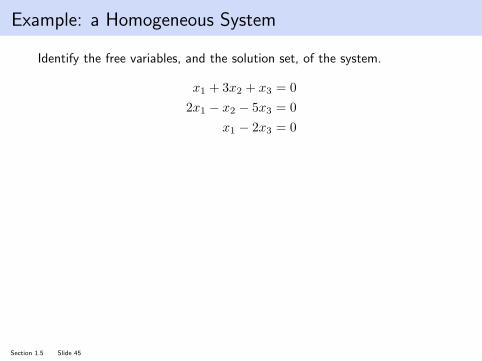
Example: a Homogeneous System

Identify the free variables, and the solution set, of the system.

x1 + 3x2 + x3 = 0

2x1 − x2 − 5x3 = 0

x1 − 2x3 = 0


Parametric Forms, Homogeneous Case

In the example on the previous slide we expressed the solution to a systemusing a vector equation. This is a parametric form of the solution.

In general, suppose the free variables for A~x = ~0 are xk, . . . , xn. Then allsolutions to A~x = ~0 can be written as

~x = xk~vk + xk+1~vk+1 + · · ·+ xn~vn

for some ~vk, . . . , ~vn. This is the parametric form of the solution.


Example 2 (non-homogeneous system)

Write the parametric vector form of the solution, and give a geometricinterpretation of the solution.

x1 + 3x2 + x3 = 9

2x1 − x2 − 5x3 = 11

x1 − 2x3 = 6

(Note that the left-hand side is the same as Example 1).


Section 1.7 : Linear Independence




1.7 : Linear Independence


• Linear independence

• Geometric interpretation of linearly independent vectors


1. Characterize a set of vectors and linear systems using the concept oflinear independence.

2. Construct dependence relations between linearly dependent vectors.

Motivating QuestionWhat is the smallest number of vectors needed in a parametric solutionto a linear system?


Linear Independence

A set of vectors {~v1, . . . , ~vk} in Rn are linearly independent if

c1~v1 + c2~v2 + · · ·+ ck~vk = ~0

has only the trivial solution. It is linearly dependent otherwise.

In other words, {~v1, . . . , ~vk} are linearly dependent if there are realnumbers c1, c2, . . . , ck not all zero so that

c1~v1 + c2~v2 + · · ·+ ck~vk = ~0


Consider the vectors:~v1, ~v2, . . . ~vk

To determine whether the vectors are linearly independent, we can setthe linear combination to the zero vector:

c1~v1 + c2~v2 + · · ·+ ck~vk =[~v1 ~v2 · · · ~vk

]c1c2...cn

= V ~c??= ~0

Linear independence: There is NO non-zero solution ~c

Linear dependence: There is a non-zero solution ~c.


Example 1

For what values of h are the vectors linearly independent?11h

,1h1

,h1

1


Example 2 (One Vector)

Suppose ~v ∈ Rn. When is the set {~v} linearly dependent?


Example 3 (Two Vectors)

Suppose ~v1, ~v2 ∈ Rn. When is the set {~v1, ~v2} linearly dependent?Provide a geometric interpretation.


Two Theorems

Fact 1. Suppose ~v1, . . . , ~vk are vectors in Rn. If k > n, then{~v1, . . . , ~vk} is linearly dependent.

Fact 2. If any one or more of ~v1, . . . , ~vk is ~0, then {~v1, . . . , ~vk} is linearlydependent.


Section 1.8 : An Introduction to LinearTransforms




1.8 : An Introduction to Linear Transforms


1. The definition of a linear transformation.

2. The interpretation of matrix multiplication as a lineartransformation.


1. Construct and interpret linear transformations in Rn (for example,interpret a linear transform as a projection, or as a shear).

2. Characterize linear transforms using the concepts ofI existence and uniquenessI domain, co-domain and range


From Matrices to Functions

Let A be an m× n matrix. We define a function

T : Rn → Rm, T (~v) = A~v

This is called a matrix transformation.

• The domain of T is Rn.

• The co-domain or target of T is Rm.

• The vector T (~x) is the image of ~x under T

• The set of all possible images T (~x) is the range.

This gives us another interpretation of A~x = ~b:

• set of equations

• augmented matrix

• matrix equation

• vector equation

• linear transformation equation


Functions from Calculus

Many of the functions we know have domain and codomain R.We canexpress the rule that defines the function sin this way:

f : R→ R f(x) = sin(x)

In calculus we often think of a function in terms of its graph, whosehorizontal axis is the domain, and the vertical axis is the codomain.

−π 0 π 2π

1sin(x)

x

y

This is ok when the domain and codomain are R. It’s hard to do whenthe domain is R2 and the codomain is R3. We would need fivedimensions to draw that graph.


Example 1

Let A =

1 10 11 1

, ~u =

[34

], ~b =

757

.

a) Compute T (~u).

b) Calculate ~v ∈ R2 so that T (~v) = ~b

c) Give a ~c ∈ R3 so there is no ~v with T (~v) = ~c

or: Give a ~c that is not in the range of T .

or: Give a ~c that is not in the span of the columns of A.


Linear Transformations

A function T : Rn → Rm is linear if

• T (~u+ ~v) = T (~u) + T (~v) for all ~u,~v in Rn.

• T (c~v) = cT (~v) for all ~v ∈ Rn, and c in R.

So if T is linear, then

T (c1~v1 + · · ·+ ck~vk) = c1T (~v1) + · · ·+ ckT (~vk)

This is called the principle of superposition. The idea is that if weknow T (~e1), . . . , T (~en), then we know every T (~v).

Fact: Every matrix transformation TA is linear.


Example 2

Suppose T is the linear transformation T (~x) = A~x. Give a shortgeometric interpretation of what T (~x) does to vectors in R2.

1) A =

[0 11 0

]

2) A =

[1 00 0

]

3) A =

[k 00 k

]for k ∈ R


Example 3

What does TA do to vectors in R3?

a) A =

1 0 00 1 00 0 0

b) A =

1 0 00 −1 00 0 1


Example 4

A linear transformation T : R2 7→ R3 satisfies

T

([10

])=

5−72

, T

([01

])=

−380

What is the matrix that represents T?


Section 1.9 : Linear Transforms



https://xkcd.com/184


1.9 : Matrix of a Linear Transformation


1. The standard vectors and the standard matrix.

2. Two and three dimensional transformations in more detail.

3. Onto and one-to-one transformations.


1. Identify and construct linear transformations of a matrix.

2. Characterize linear transformations as onto and/or one-to-one.

3. Solve linear systems represented as linear transforms.

4. Express linear transforms in other forms, such as as matrix equationsor as vector equations.


Definition: The Standard Vectors

The standard vectors in Rn are the vectors ~e1, ~e2, . . . , ~en, where:

~e1 = ~e2 = ~en =

For example, in R3,

~e1 = ~e2 = ~e3 =


A Property of the Standard Vectors

Note: if A is an m× n matrix with columns ~v1, ~v2, . . . , ~vn, then

A~ei = ~vi, for i = 1, 2, . . . , n

So multiplying a matrix by ~ei gives column i of A.

Example 1 2 34 5 67 8 9

~e2 =


The Standard Matrix

Let T : Rn 7→ Rm be a linear transformation. Then thereis a unique matrix A such that

T (~x) = A~x, ~x ∈ Rn.

In fact, A is a m×n, and its jth column is the vector T (~ej).

A =[T (~e1) T (~e2) · · · T (~en)

]

Theorem

The matrix A is the standard matrix for a linear transformation.


Rotations

Example 1What is the linear transform T : R2 → R2 defined by

T (~x) = ~x rotated counterclockwise by angle θ?


Standard Matrices in R2

• There is a long list of geometric transformations of R2 in ourtextbook, as well as on the next few slides (reflections, rotations,contractions and expansions, shears, projections, . . . )

• Please familiarize yourself with them: you are expected to memorizethem (or be able to derive them)


Two Dimensional Examples: Reflections

transformation image of unit square standard matrix

reflection through x1−axis

x1

x2

~e2

~e1

(1 00 −1

)

reflection through x2−axis

x1

x2

~e2

~e1

(−1 00 1

)


Two Dimensional Examples: Reflections


reflection through x2 = x1

x1

x2x2 = x1

~e2

~e1

(0 11 0

)

reflection through x2 = −x1

x1

x2x2 = −x1

~e2

~e1

(0 −1−1 0

)


Two Dimensional Examples: Contractions and Expansions


Horizontal Contraction

x1

x2

~e2

~e1

(k 00 1

). |k| < 1

Horizontal Expansion

x1

x2

~e2

~e1

(k 00 1

), k > 1


Two Dimensional Examples: Contractions and Expansions


Vertical Contraction

x1

x2

~e2

~e1

(1 00 k

), |k| < 1

Vertical Expansion

x1

x2

~e2

~e1

(1 00 k

), k > 1


Two Dimensional Examples: Shears


Horizontal Shear(left)

x1k < 0

x2(1 k0 1

), k < 0

Horizontal Shear(right)

x1k > 0

x2(1 k0 1

), k > 0


Two Dimensional Examples: Shears


Vertical Shear(down)

x1

x2

~e2

~e1

(1 0k 1

), k < 0

Vertical Shear(up)

x1

x2

~e2

~e1

(1 0k 1

), k > 0


Two Dimensional Examples: Projections


Projection onto the x1-axis

x1

x2

~e2

~e1

(1 00 0

)

Projection onto the x2-axis

x1

x2

~e2

~e1

(0 00 1

)


Onto

A linear transformation T : Rn → Rm is onto if for all~b ∈ Rm there is a ~x ∈ Rn so that T (~x) = ~b.

Definition

Onto is an existence property: for any ~b ∈ Rm, A~x = ~b has a solution.

Examples

• A rotation on the plane is an onto linear transformation.

• A projection in the plane is not onto.

Useful FactT is onto if and only if its standard matrix has a pivot in every row.


One-to-One

A linear transformation T : Rn → Rm is one-to-one iffor all ~b ∈ Rm there is at most one (possibly no) ~x ∈ Rn so

that T (~x) = ~b.

Definition

One-to-one is a uniqueness property, it does not assert existence for all ~b.

Examples

• A rotation on the plane is a one-to-one linear transformation.

• A projection in the plane is not one-to-one.

Useful Facts

• T is one-to-one if and only if the only solution to T (~x) = 0 is thezero vector, ~x = ~0.

• T is one-to-one if and only if the standard matrix A of T has no freevariables.


Example

Complete the matrices below by entering numbers into the missingentries so that the properties are satisfied. If it isn’t possible to do so,state why.

a) A is a 2× 3 standard matrix for a one-to-one linear transform.

A =

(1 00 1

)b) B is a 3× 2 standard matrix for an onto linear transform.

B =

1

c) C is a 3× 3 standard matrix of a linear transform that is one-to-oneand onto.

C =

1 1 1


For a linear transformation T : Rn → Rm with standardmatrix A these are equivalent statements.

1. T is onto.

2. The matrix A has columns which span Rm.

3. The matrix A has m pivotal columns.

Theorem

For a linear transformation T : Rn → Rm with standardmatrix A these are equivalent statements.

1. T is one-to-one.

2. The unique solution to T (~x) = ~0 is the trivial one.

3. The matrix A linearly independent columns.

4. Each column of A is pivotal.

Theorem


Additional Examples

1. Construct a matrix A ∈ R2×2, such that T (~x) = A~x, where T is alinear transformation that rotates vectors in R2 counterclockwise byπ/2 radians about the origin, then reflects them through the linex1 = x2.

2. Define a linear transformation by

T (x1, x2) = (3x1 + x2, 5x1 + 7x2, x1 + 3x2)

Is T one-to-one? Is T onto?


Section 2.1 : Matrix Operations

Chapter 2 : Matrix Algebra



Topics and Objectives


1. Identity and zero matrices

2. Matrix algebra (sums and products, scalar multiplies, matrix powers)

3. Transpose of a matrix


1. Apply matrix algebra, the matrix transpose, and the zero andidentity matrices, to solve and analyze matrix equations.


Definitions: Zero and Identity Matrices

1. A zero matrix is any matrix whose every entry is zero.

02×3 =

[0 0 00 0 0

], 02×1 =

[00

]2. The n× n identity matrix has ones on the main diagonal,

otherwise all zeros.

I2 =

[1 00 1

], I3 =

1 0 00 1 00 0 1

Note: any matrix with dimensions n× n is square. Zero matrices neednot be square, identity matrices must be square.


Sums and Scalar Multiples

Suppose A ∈ Rm×n, and ai,j is the element of A in row i and column j.

1. If A and B are m× n matrices, then the elements of A+B areai,j + bi,j .

2. If c ∈ R, then the elements of cA are cai,j .

For example, if[1 2 34 5 6

]+ c

[7 4 70 0 k

]=

[15 10 174 5 16

]What are the values of c and k?


Properties of Sums and Scalar Multiples

Scalar multiples and matrix addition have the expected properties.

If r, s ∈ R are scalars, and A,B,C are m× n matrices, then

1. A+ 0m×n = A

2. (A+B) + C = A+ (B + C)

3. r(A+B) = rA+ rB

4. (r + s)A = rA+ sA

5. r(sA) = (rs)A


Matrix Multiplication

Let A be a m × n matrix, and B be a n × p matrix. Theproduct is AB a m× p matrix, equal to

AB = A[~b1 · · · ~bp

]=[A~b1 · · · A~bp

]Definition

Note: the dimensions of A and B determine whether AB is defined, andwhat its dimensions will be.


Row Column Rule for Matrix Multiplication

The Row Column Rule is a convenient way to calculate the product ABthat many students have encountered in pre-requisite courses.

If A ∈ Rm×n has rows ~ai, and B ∈ Rn×p has columns ~bj ,

each element of the product C = AB is cij = ~ai ·~bj .

Row Column Method

ExampleCompute the following using the row-column method.

C = AB =

(2 01 −1

)(3 0 14 5 6

)


Properties of Matrix Multiplication

Let A,B,C be matrices of the sizes needed for the matrix multiplicationto be defined, and A is a m× n matrix.

1. (Associative) (AB)C = A(BC)

2. (Left Distributive) A(B + C) = AB +AC

3. (Right Distributive) · · ·4. (Identity for matrix multiplication) ImA = AIn

Warnings:

1. (non-commutative) In general, AB 6= BA.

2. (non-cancellation) AB = AC does not mean B = C.

3. (Zero divisors) AB = 0 does not mean that either A = 0 or B = 0.


The Associative Property

The associative property is (AB)C = A(BC). If C = ~x, then

(AB)~x = A(B~x)

Schematically:

~x

B~x

AB~x

Multiplication by BMultiplication by A

Multiplication by AB

The matrix product AB~x can be obtained by either: multiplying bymatrix AB, or by multiplying by B then by A. This means that matrixmultiplication corresponds to composition of the lineartransformations.


Proof of the Associative Law

Let A be m× n, B =[~b1 · · · ~bp

]a n× p and C =

c1...cp

a p× 1

matrix. Then,BC = c1~b1 + · · ·+ cp~bp︸︷︷︸

lin combin of cols of B

So

A(BC) = A(c1~b1 + · · ·+ cp~bp)

= c1A~b1 + · · ·+ cpA~bp (multiply by A is linear)

=[A~b1 · · · A~bp

]c1...cp

(lin combin of cols of AB)

= (AB)C.


Example

A =

[1 10 0

]Give an example of a 2× 2 matrix B that is non-commutative with A.


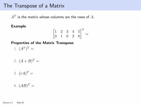
The Transpose of a Matrix

AT is the matrix whose columns are the rows of A.

Example [1 2 3 4 50 1 0 2 0

]T=

Properties of the Matrix Transpose

1. (AT )T =

2. (A+B)T =

3. (rA)T =

4. (AB)T =


Matrix Powers

For any n× n matrix and positive integer k, Ak is the product of kcopies of A.

Ak = AA . . . A

Example: Compute C8.

C =

1 0 00 2 00 0 2


Example

Define

A =

[1 00 0

], B =

[1 0 00 0 8

], C =

1 0 00 2 00 0 2

Which of these operations are defined, and what are the dimensions ofthe result?

1. A+ 3C

2. A(AB)T

3. A+ABCBT


Additional Examples

True or false:

1. For any In and any A ∈ Rn×n, (In +A)(In −A) = In −A2.

2. For any A and B in Rn×n, (A+B)2 = A2 +B2 + 2AB.


Section 2.2 : Inverse of a Matrix



”Your scientists were so preoccupied with whether or not they could,they didn’t stop to think if they should.”

- Spielberg and Crichton, Jurassic Park, 1993 film

The algorithm we introduce in this section could be used to compute aninverse of an n× n matrix. At the end of the lecture we’ll discuss some ofthe problems with our algorithm and why it can be difficult to compute a

matrix inverse.




1. Inverse of a matrix, its algebraic properties, and its relation tosolving systems of linear equations.

2. Elementary matrices and their role in calculating the matrix inverse.


1. Apply the formal definition of an inverse, and its algebraicproperties, to solve and analyze linear systems.

2. Compute the inverse of an n× n matrix, and use it to solve linearsystems.

3. Construct elementary matrices.

Motivating Question

Is there a matrix, A, such that

2 −1 0−1 2 −1

0 −1 2

A = I3?


The Matrix Inverse

A ∈ Rn×n is invertible (or non-singular) if there is aC ∈ Rn×n so that

AC = CA = In.

If there is, we write C = A−1.

Definition


The Inverse of a 2× 2 Matrix

There’s a formula for computing the inverse of a 2× 2 matrix.

The 2× 2 matrix

[a bc d

]is non-singular if and only if

ad− bc 6= 0, and then[a bc d

]−1=

1

ad− bc

[d −b−c a

]

Theorem

ExampleState the inverse of the matrix below.[

2 5−3 −7

]


The Matrix Inverse

A ∈ Rn×n has an inverse if and only if for all ~b ∈ Rn, A~x = ~bhas a unique solution. And, in this case, ~x = A−1~b.

Theorem

ExampleSolve the linear system.

3x1 + 4x2 = 7

5x1 + 6x2 = 7


Properties of the Matrix Inverse

A and B are invertible n× n matrices.

1. (A−1)−1 = A

2. (AB)−1 = B−1A−1 (Non-commutative!)

3. (AT )−1 = (A−1)T

ExampleTrue or false: (ABC)−1 = C−1B−1A−1.


An Algorithm for Computing A−1

If A ∈ Rn×n, and n > 2, how do we calculate A−1? Here’s an algorithmwe can use:

1. Row reduce the augmented matrix (A | In)

2. If reduction has form (In |B) then A is invertible and B = A−1.Otherwise, A is not invertible.

Example

Compute the inverse of A =

0 1 21 0 30 0 1

.


Why Does This Work?

We can think of our algorithm as simultaneously solving n linear systems:

A~x1 = ~e1

A~x2 = ~e2

...

A~xn = ~en

Each column of A−1 is A−1~ei = ~xi.

Over the next few slides we explore another explanation for how ouralgorithm works. This other explanation uses elementary matrices.


Elementary Matrices

An elementary matrix, E, is one that differs by In by one row operation.Recall our elementary row operations:

1. swap rows

2. multiply a row by a non-zero scalar

3. add a multiple of one row to another

We can represent each operation by a matrix multiplication with anelementary matrix.


Example

Suppose

E

1 1 1−2 1 00 0 1

=

1 1 10 3 20 0 1

By inspection, what is E? How does it compare to I3?


Theorem

Returning to understanding why our algorithm works, we apply asequence of row operations to A to obtain In:

(Ek · · ·E3E2E1)A = In

Thus, Ek · · ·E3E2E1 is the inverse matrix we seek.

Our algorithm for calculating the inverse of a matrix is the result of thefollowing theorem.

Matrix A is invertible if and only if it is row equivalent to theidentity. In this case, the any sequence of elementary row op-erations that transforms A into I, applied to I, generates A−1.

Theorem


Using The Inverse to Solve a Linear System

• We could use A−1 to solve a linear system,

A~x = ~b

We would calculate A−1 and then:

• As our textbook points out, A−1 is seldom used: computing it cantake a very long time, and is prone to numerical error.

• So why did we learn how to compute A−1? Later on in this course,we use elementary matrices and properties of A−1 to derive results.

• A recurring theme of this course: just because we can do somethinga certain way, doesn’t that we should.


Section 2.3 : Invertible Matrices



“A synonym is a word you use when you can’t spell the other one.”- Baltasar Gracian

The theorem we introduce in this section of the course gives us many waysof saying the same thing. Depending on the context, some will be more

convenient than others.




1. The invertible matrix theorem, which is a review/synthesis of manyof the concepts we have introduced.


1. Characterize the invertibility of a matrix using the Invertible MatrixTheorem.

2. Construct and give examples of matrices that are/are not invertible.

Motivating QuestionWhen is a square matrix invertible? Let me count the ways!


The Invertible Matrix Theorem

Invertible matrices enjoy a rich set of equivalent descriptions.

TheoremLet A be an n× n matrix. These statements are all equivalent.

a) A is invertible.

b) A is row equivalent to In.

c) A has n pivotal columns. (All columns are pivotal.)

d) A~x = ~0 has only the trivial solution.

e) The columns of A are linearly independent.

f) The linear transformation ~x 7→ A~x is one-to-one.

g) The equation A~x = ~b has a solution for all ~b ∈ Rn.

h) The columns of A span Rn.

i) The linear transformation ~x 7→ A~x is onto.

j) There is a n× n matrix C so that CA = In. (A has a left inverse.)

k) There is a n×n matrix D so that AD = In. (A has a right inverse.)

l) AT is invertible.Section 2.3 Slide 113

Invertibility and Composition

The diagram below gives us another perspective on the role of A−1.

~x

A~x

Multiplication by A

Multiplication by A−1

The matrix inverse A−1 transforms Ax back to ~x. This is because:

A−1(A~x) = (A−1A)~x =


The Invertible Matrix Theorem: Final Notes

• Items j and k of the invertible matrix theorem (IMT) lead us directlyto the following theorem.

If A and B are n×n matrices and AB = I, then A andB are invertible, and B = A−1 and A = B−1.

Theorem

• The IMT is a set of equivalent statements. They divide the set of allsquare matrices into two separate classes: invertible, andnon-invertible.

• As we progress through this course, we will be able to add additionalequivalent statements to the IMT (that deal with determinants,eigenvalues, etc).


Example 1

Is this matrix invertible? 1 0 −23 1 −2−5 −1 9


Example 2

If possible, fill in the missing elements of the matrices below withnumbers so that each of the matrices are singular. If it is not possible todo so, state why.

1 0 11 10 0 1

,

1 10 1 10 0 1

,

1 0 00 1 10 1


Matrix Completion Problems

• The previous example is an example of a matrix completion problem(MCP).

• MCPs are great questions for recitations, midterms, exams.• the Netflix Problem is another example of an MCP.

Given a ratings matrix in which each entry (i, j) representsthe rating of movie j by customer i if customer i has watchedmovie j, and is otherwise missing, predict the remaining matrixentries in order to make recommendations to customers on whatto watch next.

Students are not expected to be familiar with this material. It’s presented to

motivate matrix completion.Section 2.3 Slide 118

Section 2.4 : Partitioned Matrices



“Mathematics is not about numbers, equations, computations, oralgorithms. Mathematics is about understanding.”

- William Paul Thurston

Multiple perspectives of the same concept is a theme of this course; eachperspective deepens our understanding. In this section we explore another

way of representing matrices and their algebra that gives us another way ofthinking about them.




1. Partitioned matrices (or block matrices)


1. Apply partitioned matrices to solve problems regarding matrixinvertibility and matrix multiplication.


What is a Partitioned Matrix?

ExampleThis matrix: 3 1 4 1 0

1 6 1 0 10 0 0 4 2

can also be written as:

[3 1 41 6 1

] [1 00 1

][0 0 0

] [4 2

] =

[A1,1 A1,2

A2,1 A2,2

]

We partitioned our matrix into four blocks, each of which has differentdimensions.


Another Example of a Partitioned Matrix

Example: The reduced echelon form of a matrix. We can use apartitioned matrix to

1 0 0 0 ∗ · · · ∗0 1 0 0 ∗ · · · ∗0 0 1 0 ∗ · · · ∗0 0 0 1 ∗ · · · ∗0 0 0 0 0 · · · 00 0 0 0 0 · · · 0

=

[I4 F0 0

]

This is useful when studying the null space of A, as we will see later inthis course.


Row Column Method

Recall that a row vector times a column vector (of the right dimensions)is a scalar. For example,

[1 1 1

] 102

=

This is the row column matrix multiplication method from Section 2.1.

Let A be m × n and B be n × p matrix. Then, the (i, j)entry of AB is

rowiA · colj B.

This is the Row Column Method for matrix multiplication.

Theorem

Partitioned matrices can be multiplied using this method, as if each blockwere a scalar (provided each block has appropriate dimensions).


Example of Row Column Method

Recall, using our formula for a 2× 2 matrix,

[a b0 c

]−1= 1

ac

[c −b0 a

].

Example: Suppose A ∈ Rn×n, B ∈ Rn×n, and C ∈ Rn×n are invertible

matrices. Construct the inverse of

[A B0 C

].


The Strassen Algorithm: An impressive use of partitionedmatrices

Naive Multiplication of two n× n matrices A and B requires n3

arithmetic steps. Strassen’s algorithm partitions the matrices, makes avery clever sequence of multiplications, additions, to reduce thecomputation to n2.803... steps.

Students aren’t expected to be familiar with this material. It’s presented to

motivate matrix partitioning.


The Fast Fourier Transform (FFT)

The FFT is an essential algorithm of modern technology that usespartitioned matrices recursively.

G0 =[1], Gn+1 =

[Gn −Gn

Gn Gn

]

The recursive structure of the matrixmeans that it can be computed innearly linear time. This is anincredible saving over the generalcomplexity of n3. It means that wecan compute Gnx, and G−1n veryquickly.

Students aren’t expected to be familiar with this material. It is presented to

motivate matrix partitioning.


Section 2.5 : Matrix Factorizations



“Mathematical reasoning may be regarded rather schematically as theexercise of a combination of two facilities, which we may call intuition and

ingenuity.” - Alan Turing

The use of the LU Decomposition to solve linear systems was one of theareas of mathematics that Turing helped develop.




1. The LU factorization of a matrix

2. Using the LU factorization to solve a system

3. Why the LU factorization works


1. Compute an LU factorization of a matrix.

2. Apply the LU factorization to solve systems of equations.

3. Determine whether a matrix has an LU factorization.


Motivation

• Recall that we could solve A~x = ~b by using

~x = A−1~b

• This requires computation of the inverse of an n× n matrix, whichis especially difficult for large n.

• Instead we could solve A~x = ~b with Gaussian Elimination, but this isnot efficient for large n

• There are more efficient and accurate methods for solving linearsystems that rely on matrix factorizations.


Matrix Factorizations

• A matrix factorization, or matrix decomposition is a factorizationof a matrix into a product of matrices.

• Factorizations can be useful for solving A~x = ~b, or understandingthe properties of a matrix.

• We explore a few matrix factorizations throughout this course.

• In this section, we factor a matrix into lower and into uppertriangular matrices.


Triangular Matrices

• A rectangular matrix A is upper triangular if ai,j = 0 for i > j.Examples:

(1 5 00 2 4

),

1 0 0 10 2 1 00 0 1 00 0 0 1

,

2000

• A rectangular matrix A is lower triangular if ai,j = 0 for i < j.

Examples:

(1 0 03 2 0

),

3 0 0 01 1 0 00 0 1 00 2 0 1

,

1212

Ask: Can you name a matrix that is both upper and lower triangular?


The LU Factorization

If A is an m × n matrix that can be row reduced to echelon formwithout row exchanges, then A = LU . L is a lower triangular m×mmatrix with 1’s on the diagonal, U is an echelon form of A.

Theorem

Example: If A ∈ R3×2, the LU factorization has the form:

A = LU =

1 0 0∗ 1 0∗ ∗ 1

∗ ∗0 ∗0 0


Why We Can Compute the LU Factorization

Suppose A can be row reduced to echelon form U without interchangingrows. Then,

Ep · · ·E1A = U

where the Ej are matrices that perform elementary row operations. Theyhappen to be lower triangular and invertible, e.g.1 0 0

0 1 02 0 1

−1 =

1 0 00 1 0−2 0 1

Therefore,

A = E−11 · · ·E−1p︸︷︷︸=L

U = LU.


Using the LU Decomposition

Goal: given A and ~b, solve A~x = ~b for ~x.

Algorithm: construct A = LU , solve A~x = LU~x = ~b by:

1. Forward solve for ~y in L~y = ~b.

2. Backwards solve for x in U~x = ~y.

Example: Solve the linear system whose LU decomposition is given.

A = LU =

1 0 0 01 1 0 00 2 1 00 0 1 1

1 0 00 2 10 0 20 0 0

, ~b =

2320


An Algorithm for Computing LU

To compute the LU decomposition:

1. Reduce A to an echelon form U by a sequence of row replacementoperations, if possible.

2. Place entries in L such that the same sequence of row operationsreduces L to I.

Note that

• In MATH 1554, the only row replacement operation we can use is toreplace a row with a multiple of a row above it.

• More advanced linear algebra courses address this limitation.

Example: Compute the LU factorization of A.

A =

4 −3 −1 5−16 12 2 −17

8 −6 −12 22


Summary

• To solve A~x = LU~x = ~b,

1. Forward solve for ~y in L~y = ~b.2. Backwards solve for ~x in U~x = ~y.

• To compute the LU decomposition:

1. Reduce A to an echelon form U by a sequence of row replacementoperations, if possible.

2. Place entries in L such that the same sequence of row operationsreduces L to I.

• The textbook offers a different explanation of how to construct theLU decomposition that students may find helpful.

• Another explanation on how to calculate the LU decomposition thatstudents may find helpful is available from MIT OpenCourseWare:www.youtube.com/watch?v=rhNKncraJMk


Section 2.6 : The Leontif Input-Output Model



“Computers and robots replace humans in the exercise of mental functionsin the same way as mechanical power replaced them in the performance of

physical tasks.” - Wassily Leontif, 1983

Students in this course are of course required to demonstrate anunderstanding of underlying concepts behind procedures and algorithms.

This is in part because computers are continuing to take on a much largerrole in performing calculations.




1. The Leontief Input-Output model, as a simple example of a modelof an economy.


1. Apply matrix algebra and inverses to solve and analyze LeontifInput-Output problems.

Motivating QuestionAn economy consisting of 3 sectors: agriculture, manufacturing, andenergy. The output of one sector is absorbed by all the sectors. If there isan increase in demand for energy, how does this impact the economy?


Example: An Economy with Two Sectors

E

W

External demands

This economy contains two sectors.

1. electricity (E)

2. water (W)

The “external demands” is another part of the economy, which does notproduce E and W.

How might we represent this economy with a set of linear equations?


The Leontif Model: Internal Consumption

Suppose economy has N sectors, with outputs measured by ~x ∈ RN .

~x = output vector

xi = element i of vector ~x = number of units produced by sector i

The consumption matrix, C, describes how units are consumed bysectors to produce output. Two equivalent ways of defining C:

• Sector j requires a proportion of the units created by sector i. Callthat ci,jxi

• Sector i sends a proportion of its units to sector j. Call that ci,jxi

Elements of C are ci,j , with ci,j ∈ [0, 1], and

C~x = units consumed

~x− C~x = units left after internal consumption


Example 1

An economy contains three sectors, E, W, M. For every 100 units ofoutput,

• E requires 20 units from E, 10 units from W, and 10 units from M

• W requires 0 units from E, 20 units from W, and 10 units from M

• M requires 0 units from E, 0 units from W, and 20 units from M

Construct the consumption matrix for this economy.

E W

M

20%10%

20%

10% 10%

20%


Solution: Creating C

Our consumption matrix is

C =1

10

2 0 01 2 01 1 2

Note:

• total output for each sector is the sum along the outgoing edges foreach sector, which generates rows of C

• elements of C represent percentages with no units, they have valuesbetween 0 and 1

• our output vector has units


The Leontif Model: Demand

There is also an external demand given by ~d ∈ RN . We ask if there is an~x such that

~x− C~x = ~d

Solving for ~x yields~x = (I − C)−1~d

This is the Leontief Input-Output Model.


Example 1 Revisited

Now suppose there is an external demand: what production level isrequired to satisfy a final demand of 80 units of E, 70 units of W, and160 unites of M?

E W

MD

20%

80 units

10%20%

10%10%

20%160 units

70 units


Solution

The production level would be found by solving:

~x− C~x = ~d

(I − C)~x = ~d

1

10

8 0 0−1 8 0−1 −1 8

~x =

8070160

8x1 = 800 ⇒ x1 = 100

−x1 + 8x2 = 700 ⇒ x2 = 100

−x1 − x2 + 8x3 = 1600 ⇒ x3 = 1800/8 = 225

The output that balances demand with internal consumption is

~x =

100100225

.


The Importance of (I − C)−1

For the example above

(I − C)−1 ≈

1.25 0 00.15 1.25 00.18 0.17 1.25

The entries of (I − C)−1 = B have this meaning: if the final demand

vector ~d increases by one unit in the jth place, the column vector bj isthe additional output required from other sectors.

So to meet an increase in demand for M by one unit, requires 1.25 of oneadditional units from M to meet internal consumption.


Section 2.7 : Computer Graphics






1. Homogeneous coordinates in 2D and 3D2. Translations and composite transforms in 2D and 3D


1. Construct a data matrix to represent points in R2 and R3 usinghomogeneous coordinates.

2. Construct transformation matrices to represent compositetransforms in 2D and 3D using homogeneous coordinates.

3. Apply composite transforms and data matrices to transform pointsin R3

In the interest of time, students are not expected to be familiar withperspective projections.

Motivating QuestionHow can we represent translations using linear transforms?


Homogenous Coordinates

Translations of points in Rn does not correspond directly to a lineartransform. Homogeneous coordinates are used model translationsusing matrix multiplication.

Each point (x, y) in R2 can be identified with the point (x, y,H),H 6= 0, on the plane in R3 that lies H units above the xy-plane.

Homogeneous Coordinates in R2

Note: we often we set H = 1.

Example: A translation of the form (x, y)→ (x+ h, y + k) can berepresented as a matrix multiplication with homogeneous coordinates: 1 0 h

0 1 k0 0 1

xy1

=

x+ hy + k

1


A Composite Transform with Homogeneous Coordinates

Triangle S is determined by three data points, (1, 1), (2, 4), (3, 1).

Transform T rotates points by π/2 radians counterclockwise about thepoint (0, 1).

a) Represent the data with a matrix, D. Use homogeneous coordinates.

b) Use matrix multiplication to determine the image of S under T .

c) Sketch S and its image under T .


3D Homogeneous Coordinates

Homogeneous coordinates in 3D are analogous to our 2D coordinates.

(X,Y, Z,H) are homogeneous coordinates for (x, y, z)in R3, H 6= 0, and

x =X

H, y =

Y

H, z =

Z

H

Homogeneous Coordinates in R3

For example, (a, b, c, 1) and (3a, 3b, 3c, 3) are both homogeneouscoordinates for the point (a, b, c).


3D Transformation Matrices

Construct matrices for the following transformations.

a) A rotation in R3 about the y-axis by π radians.

b) A translation specified by the vector ~p =

−234

.


Section 2.8 : Subspaces of Rn






1. Subspaces, Column space, and Null spaces

2. A basis for a subspace.


1. Determine whether a set is a subspace.

2. Determine whether a vector is in a particular subspace, or find avector in that subspace.

3. Construct a basis for a subspace (for example, a basis for Col(A))

Motivating QuestionGiven a matrix A, what is the set of vectors ~b for which we can solveA~x = ~b?


Subsets of Rn

A subset of Rn is any collection of vectors that are in Rn.

Definition


Subspaces in Rn

A subset H of Rn is a subspace if it is closed under scalar multipliesand vector addition. That is: for any c ∈ R and for ~u,~v ∈ H,

1. c ~u ∈ H2. ~u+ ~v ∈ H

Definition

Note that condition 1 implies that the zero vector must be in H.Example 1: Which of the following subsets could be a subspace of R2?


The Column Space and the Null Space of a Matrix

Recall: for ~v1, . . . , ~vp ∈ Rn, that Span{~v1, . . . , ~vp} is:

This is a subspace, spanned by ~v1, . . . , ~vp.

Given an m× n matrix A =[~a1 · · · ~an

]1. The column space of A, ColA, is the subspace of Rm

spanned by ~a1, . . . ,~an.

2. The null space of A, NullA, is the subspace of Rn spannedby the set of all vectors ~x that solve A~x = ~0.

Definition


Example

Is ~b in the column space of A?

A =

1 −3 −4−4 6 −2−3 7 6

∼1 −3 −4

0 −6 −180 0 0

, ~b =

33−4


Example 2 (continued)

Using the matrix on the previous slide: is ~v in the null space of A?

~v =

−5λ−3λλ

, λ ∈ R


Basis

A basis for a subspace H is a set of linearly independentvectors in H that span H.

Definition

Example

The set H = {

x1x2x3x4

∈ R4 | x1 + 2x2 + x3 + 5x4 = 0} is a subspace.

a) H is a null space for what matrix A?

b) Construct a basis for H.


Example

Construct a basis for NullA and a basis for ColA.

A =

−3 6 −1 01 −2 2 02 −4 5 0

∼1 −2 0 0

0 0 1 00 0 0 0


Additional Example

Let V =

{(ab

)∈ R2 | ab = 0

}.

1. Give an example of a vector that is in V .

2. Give an example of a vector that is not in V .

3. Is the zero vector in V ?

4. Is V a subspace?


Section 2.9 : Dimension and Rank






1. Coordinates, relative to a basis.

2. Dimension of a subspace.

3. The Rank of a matrix


1. Calculate the coordinates of a vector in a given basis.

2. Characterize a subspace using the concept of dimension (orcardinality).

3. Characterize a matrix using the concepts of rank, column space, nullspace.

4. Apply the Rank, Basis, and Matrix Invertibility theorems to describematrices and subspaces.


Choice of Basis

Key idea: There are many possible choices of basis for a subspace. Ourchoice can give us dramatically different properties.

Example: sketch ~b1 +~b2 for the two different coordinate systems below.

~b2

~b1

~b2

~b1


Coordinates

DefinitionLet B = {~b1, . . . ,~bp} be a basis for a subspace H. If ~x is in H, thencoordinates of ~x relative B are the weights (scalars) c1, . . . , cp so that

~x = c1~b1 + · · ·+ cp~bp

And

[x]B =

c1...cp

is the coordinate vector of ~x relative to B, or the B-coordinatevector of ~x


Example 1

Let ~v1 =

101

, ~v2 =

111

, and ~x =

535

. Verify that ~x is in the span of

B = {~v1, ~v2}, and calculate [~x]B.


Dimension

DefinitionThe dimension (or cardinality) of a non-zero subspace H, dimH, is thenumber of vectors in a basis of H. We define dim{0} = 0.

TheoremAny two choices of bases B1 and B2 of a non-zero subspace H have thesame dimension.

Examples:

1. dimRn =

2. H = {(x1, . . . , xn) : x1 + · · ·+ xn = 0} has dimension

3. dim(NullA) is the number of

4. dim(ColA) is the number of


Rank

The rank of a matrix A is the dimension of its column space.

Definition

Example 2: Compute rank(A) and dim(Nul(A)).2 5 −3 −4 84 7 −4 −3 96 9 −5 2 40 −9 6 5 −6

∼ · · · ∼

2 5 −3 −4 80 −3 2 5 −70 0 0 4 −60 0 0 0 0


Rank, Basis, and Invertibility Theorems

Theorem (Rank Theorem)If a matrix A has n columns, then RankA+ dim(NulA) = n.

Theorem (Basis Theorem)Any two bases for a subspace have the same dimension.

Theorem (Invertibility Theorem)Let A be a n× n matrix. These conditions are equivalent.

1. A is invertible.

2. The columns of A are a basis for Rn.

3. ColA = Rn.

4. rankA = dim(ColA) = n.

5. NullA = {0}.


Examples

If possible give an example of a 2× 3 matrix A, that is in RREF and hasthe given properties.

a) rank(A) = 3

b) rank(A) = 2

c) dim(Null(A)) = 2

d) NullA = {0}


Section 3.1 : Introduction to Determinants

Chapter 3 : Determinants





1. The definition and computation of a determinant

2. The determinant of triangular matrices


1. Compute determinants of n× n matrices using a cofactor expansion.

2. Apply theorems to compute determinants of matrices that haveparticular structures.


A Definition of the Determinant

Suppose A is n× n and has elements aij .

1. If n = 1, A = [a11], and has determinant detA = a11.

2. Inductive case: for n > 1,

detA = a11 detA11 − a12 detA12 + · · ·+ (−1)1+na1n detA1n

where Aij is the submatrix obtained by eliminating row i andcolumn j of A.

Example

A =

⇒ A2,3 =


Example 1

Compute det

[a bc d

].


Example 2

Compute det

1 −5 02 4 −10 2 0

=

∣∣∣∣∣∣1 −5 02 4 −10 2 0

∣∣∣∣∣∣.


Cofactors

Cofactors give us a more convenient notation for determinants.

The (i, j) cofactor of an n× n matrix A is

Cij = (−1)i+j detAij

Definition: Cofactor

The pattern for the negative signs is+ − + − . . .− + − + . . .+ − + − . . .− + − + . . ....

......

...


The determinant of a matrix A can be computed down anyrow or column of the matrix. For instance, down the jth

column, the determinant is

detA = a1jC1j + a2jC2j + · · ·+ anjCnj .

Theorem

This gives us a way to calculate determinants more efficiently.


Example 3

Compute the determinant of

5 4 3 20 1 2 00 −1 1 00 1 1 3

.


Triangular Matrices

If A is a triangular matrix then

detA = a11a22a33 · · · ann.

Theorem

Example 4Compute the determinant of the matrix. Empty elements are zero.

2 12 1

2 12 1

2 12 1

2


Computational Efficiency

Note that computation of a co-factor expansion for an N ×N matrixrequires roughly N ! multiplications.

• A 10× 10 matrix requires roughly 10! = 3.6 million multiplications

• A 20× 20 matrix requires 20! ≈ 2.4× 1018 multiplications

Co-factor expansions may not be practical, but determinants are stilluseful.

• We will explore other methods for computing determinants that aremore efficient.

• Determinants are very useful in multivariable calculus for solvingcertain integration problems.


Section 3.2 : Properties of the Determinant



“A problem isn’t finished just because you’ve found the right answer.”- Yoko Ogawa

We have a method for computing determinants, but without some of thestrategies we explore in this section, the algorithm can be very inefficient.




• The relationships between row reductions, the invertibility of amatrix, and determinants.


1. Apply properties of determinants (related to row reductions,transpose, and matrix products) to compute determinants.

2. Use determinants to determine whether a square matrix is invertible.


Row Operations

• We saw how determinants are difficult or impossible to computewith a cofactor expansion for large N .

• Row operations give us a more efficient way to computedeterminants.

Let A be a square matrix.1. If a multiple of a row of A is added to another row to

produce B, then detB = detA.

2. If two rows are interchanged to produce B, thendetB = −detA.

3. If one row of A is multiplied by a scalar k to produceB, then detB = k detA.

Theorem: Row Operations and the Determinant


Example 1 Compute

∣∣∣∣∣∣1 −4 2−2 8 −9−1 7 0

∣∣∣∣∣∣


Invertibility

Important practical implication: If A is reduced to echelon form, by rinterchanges of rows and columns, then

|A| =

{(−1)r × (product of pivots), when A is invertible

0, when A is singular.


Example 2 Compute the determinant∣∣∣∣∣∣∣∣0 1 2 −12 5 −7 30 3 6 2−2 −5 4 2

∣∣∣∣∣∣∣∣


Properties of the Determinant

For any square matrices A and B, we can show the following.

1. detA = detAT .

2. A is invertible if and only if detA 6= 0.

3. det(AB) = detA · detB.


Additional Example (if time permits)

Use a determinant to find all values of λ such that matrix C is notinvertible.

C =

5 0 00 0 11 1 0

− λI3



Determine the value of

detA = det

0 2 0

1 1 21 1 3

8 .


Section 3.3 : Volume, Linear Transformations






1. Relationships between area, volume, determinants, and lineartransformations.


1. Use determinants to compute the area of a parallelogram, or thevolume of a parallelepiped, possibly under a given lineartransformation.

Students are not expected to be familiar with Cramer’s rule.


Determinants, Area and Volume

In R2, determinants give us the area of a parallelogram.

area of parallelogram = det

(a cb d

)= ad− bc.


Determinants as Area, or Volume

The volume of the parallelpiped spanned by the columns ofan n× n matrix A is |detA|.

Theorem

Key Geometric Fact (which works in any dimension). The area of

the parallelogram spanned by two vectors ~a,~b is equal to the areaspanned by ~a, c~a+~b, for any scalar c.


Example 1

Calculate the area of the parallelogram determined by the points(−2,−2), (0, 3), (4,−1), (6, 4)


Linear Transformations

If TA : Rn 7→ Rn, and S is some parallelogram in Rn, then

volume (TA(S)) = |det(A)| · volume(S)

Theorem

An example that applies this theorem is given in this week’s worksheets.


Section 4.9 : Applications to Markov Chains

Chapter 4 : Vector Spaces





1. Markov chains

2. Steady-state vectors

3. Convergence


1. Construct stochastic matrices and probability vectors.

2. Model and solve real-world problems using Markov chains (e.g. -find a steady-state vector for a Markov chain)

3. Determine whether a stochastic matrix is regular.


Example 1

• A small town has two libraries, A and B.

• After 1 month, among the books checked out of A,I 80% returned to AI 20% returned to B

• After 1 month, among the books checked out of B,I 30% returned to AI 70% returned to B

If both libraries have 1000 books today, how many books does eachlibrary have after 1 month? After one year? After n months? A place tosimulate this is http://setosa.io/markov/index.html

A B

0.2

0.8

0.3

0.7


http://setosa.io/markov/index.html

Example 1 Continued

The books are equally divided by between the two branches, denoted by

~x0 =

[.5.5

]. What is the distribution after 1 month, call it ~x1? After two

months?

After k months, the distribution is ~xk, which is what in terms of ~x0?


Markov Chains

A few definitions:

• A probability vector is a vector, ~x, with non-negative elements thatsum to 1.

• A stochastic matrix is a square matrix, P , whose columns areprobability vectors.

• A Markov chain is a sequence of probability vectors ~xk, and astochastic matrix P , such that:

~xk+1 = P~xk, k = 0, 1, 2, . . .

• A steady-state vector for P is a vector ~q such that P~q = ~q.


Example 2

Determine a steady-state vector for the stochastic matrix(.8 .3.2 .7

)


Convergence

We often want to know what happens to a process,

~xk+1 = P~xk, k = 0, 1, 2, . . .

as k →∞.

Definition: a stochastic matrix P is regular if there is some k such thatP k only contains strictly positive entries.

If P is a regular stochastic matrix, then P has a unique steady-state vector ~q, and ~xk+1 = P~xk converges to ~q as k →∞.

Theorem


Stochastic Vectors in the Plane

The stochastic vectors in the plane are the line segment below, and astochastic matrix maps stochastic vectors to themselves. Iterates P k~x0converge to the steady state.

1

1

~x∞

Steady State Vector

~x0

~x1

~x2

~x3

P k −→[~x∞ ~x∞

]


Example 3

A car rental company has 3 rental locations, A, B, and C. Cars can bereturned at any location. The table below gives the pattern of rental andreturns for a given week.

rented fromA B C

returned toA .8 .1 .2B .2 .6 .3C .0 .3 .5

There are 10 cars at each location today.

a) Construct a stochastic matrix, P , for this problem.

b) What happens to the distribution of cars after a long time? Youmay assume that P is regular.


A B

C

.2

.8

.1

.6

.3.2

.5

.3

P =

.8 .1 .2.2 .6 .3.0 .3 .5


The Stochastic vectors in R3, are vectors

st

1− s− t

, where

0 ≤ s, t ≤ 1 and s+ t ≤ 1. P ‘contracts’ stochastic vectors to x∞.

(1, 0, 0)

(0, 1, 0)(0, 0, 1)

x∞


Section 5.1 : Eigenvectors and Eigenvalues

Chapter 5 : Eigenvalues and Eigenvectors





1. Eigenvectors, eigenvalues, eigenspaces

2. Eigenvalue theorems


1. Verify that a given vector is an eigenvector of a matrix.

2. Verify that a scalar is an eigenvalue of a matrix.

3. Construct an eigenspace for a matrix.

4. Apply theorems related to eigenvalues (for example, to characterizethe invertibility of a matrix).


Eigenvectors and Eigenvalues

If A ∈ Rn×n, and there is a ~v 6= ~0 in Rn, and

A~v = λ~v

then ~v is an eigenvector for A, and λ ∈ C is the correspondingeigenvalue.

Note that

• We will only consider square matrices.

• If λ ∈ R, thenI when λ > 0, A~v and ~v point in the same directionI when λ < 0, A~v and ~v point in opposite directions

• Even when all entries of A and ~v are real, λ can be complex (arotation of the plane has no real eigenvalues.)

• We explore complex eigenvalues in Section 5.5.


Example 1

Which of the following are eigenvectors of A =

(1 11 1

)? What are the

corresponding eigenvalues?

a) ~v1 =

(11

)

b) ~v2 =

(1−1

)

c) ~v3 =

(00

)


Example 2

Confirm that λ = 3 is an eigenvalue of A =

(2 −4−1 −1

).


Eigenspace

Suppose A ∈ Rn×n. The eigenvectors for a given λ span asubspace of Rn called the λ-eigenspace of A.

Definition

Note: the λ-eigenspace for matrix A is Nul(A− λI).

Example 3Construct a basis for the eigenspaces for the matrix whose eigenvaluesare given, and sketch the eigenvectors.(

5 −63 −4

), λ = −1, 2


Theorems

Proofs for the most these theorems are in Section 5.1. If time permits,we will explain or prove all/most of these theorems in lecture.

1. The diagonal elements of a triangular matrix are its eigenvalues.

2. A invertible ⇔ 0 is not an eigenvalue of A.

3. Stochastic matrices have an eigenvalue equal to 1.

4. If ~v1, ~v2, . . . , ~vk are eigenvectors that correspond to distincteigenvalues, then ~v1, ~v2, . . . , ~vk are linearly independent.


Warning!

We can’t determine the eigenvalues of a matrix from its reduced form.

Row reductions change the eigenvalues of a matrix.

Example: suppose A =

[1 11 1

]. The eigenvalues are λ = 2, 0, because

A

[11

]=

[1 11 1

] [11

]=

A

[1−1

]=

[1 11 1

] [1−1

]=

• But the reduced echelon form of A is:

• The reduced echelon form is triangular, and its eigenvalues are:


Section 5.2 : The Characteristic Equation






1. The characteristic polynomial of a matrix

2. Algebraic and geometric multiplicity of eigenvalues

3. Similar matrices


1. Construct the characteristic polynomial of a matrix and use it toidentify eigenvalues and their multiplicities.

2. Characterize the long-term behaviour of dynamical systems usingeigenvalue decompositions.


The Characteristic Polynomial

Recall:

λ is an eigenvalue of A ⇔ (A− λI) is not

Therefore, to calculate the eigenvalues of A, we can solve

det(A− λI) =

The quantity det(A− λI) is the characteristic polynomial of A.

The quantity det(A− λI) = 0 is the characteristic equation of A.

The roots of the characteristic polynomial are the of A.


Example

The characteristic polynomial of A =

(5 22 1

)is:

So the eigenvalues of A are:


Characteristic Polynomial of 2× 2 Matrices

Express the characteristic equation of

M =

(a bc d

)in terms of its determinant. What is the equation when M is singular?


Algebraic Multiplicity

The algebraic multiplicity of an eigenvalue is its multiplicityas a root of the characteristic polynomial.

Definition

ExampleCompute the algebraic multiplicities of the eigenvalues for the matrix

1 0 0 00 0 0 00 0 −1 00 0 0 0


Geometric Multiplicity

The geometric multiplicity of an eigenvalue λ is the dimensionof Null(A− λI).

Definition

1. Geometric multiplicity is always at least 1. It can be smaller thanalgebraic multiplicity.

2. Here is the basic example: (0 10 0

)λ = 0 is the only eigenvalue. Its algebraic multiplicity is 2, but thegeometric multiplicity is 1.


Example

Give an example of a 4× 4 matrix with λ = 0 the only eigenvalue, butthe geometric multiplicity of λ = 0 is one.


Recall: Long-Term Behavior of Markov Chains

Recall:

• We often want to know what happens to a Markov Chain

~xk+1 = P~xk, k = 0, 1, 2, . . .

as k →∞.

• If P is regular, then there is a

Now lets ask:

• If we don’t know whether P is regular, what else might we do todescribe the long-term behavior of the system?

• What can eigenvalues tell us about the behavior of these systems?


Example: Eigenvalues and Markov Chains

Consider the Markov Chain:

~xk+1 = P~xk =

(0.6 0.40.4 0.6

)~xk, k = 0, 1, 2, 3, . . . , ~x0 =

(10

)This system can be represented schematically with two nodes, A and B:

A B

0.4

0.6

0.4

0.6

Goal: use eigenvalues to describe the long-term behavior of our system.


What are the eigenvalues of P?

What are the corresponding eigenvectors of P?


Use the eigenvalues and eigenvectors of P to analyze the long-termbehaviour of the system. In other words, determine what ~xk tends to ask →∞.


Similar Matrices

Two n×n matrices A and B are similar if there is a matrix P so thatA = PBP−1.

Definition

If A and B similar, then they have the same characteristic polynomial.

Theorem

If time permits, we will explain or prove this theorem in lecture. Note:

• Our textbook introduces similar matrices in Section 5.2, but doesn’thave exercises on this concept until 5.3.

• Two matrices, A and B, do not need to be similar to have the sameeigenvalues. For example,(

0 10 0

)and

(0 00 0

)


Additional Examples (if time permits)

1. True or false.

a) If A is similar to the identity matrix, then A is equal to the identitymatrix.

b) A row replacement operation on a matrix does not change itseigenvalues.

2. For what values of k does the matrix have one real eigenvalue withalgebraic multiplicity 2? (

−3 k2 −6

)


Section 5.3 : Diagonalization



Motivation: it can be useful to take large powers of matrices, for exampleAk, for large k.

But: multiplying two n× n matrices requires roughly n3 computations. Isthere a more efficient way to compute Ak?



Topics

1. Diagonal, similar, and diagonalizable matrices

2. Diagonalizing matrices

Learning ObjectivesFor the topics covered in this section, students are expected to be able todo the following.

1. Determine whether a matrix can be diagonalized, and if possiblediagonalize a square matrix.

2. Apply diagonalization to compute matrix powers.


Diagonal Matrices

A matrix is diagonal if the only non-zero elements, if any, are on themain diagonal.

The following are all diagonal matrices.[2 00 2

],[2], In,

[0 00 0

]We’ll only be working with diagonal square matrices in this course.


Powers of Diagonal Matrices

If A is diagonal, then Ak is easy to compute. For example,

A =

(3 00 0.5

)

A2 =

Ak =

But what if A is not diagonal?


Diagonalization

Suppose A ∈ Rn×n. We say that A is diagonalizable if it is similar to adiagonal matrix, D. That is, we can write

A = PDP−1


Diagonalization

If A is diagonalizable ⇔ A has n linearly independent eigenvectors.

Theorem

Note: the symbol ⇔ means “ if and only if ”.

Also note that A = PDP−1 if and only if

A = [~v1 ~v2 · · ·~vn]

λ1

λ2. . .

λn

[~v1 ~v2 · · ·~vn]−1

where ~v1, . . . , ~vn are linearly independent eigenvectors, and λ1, . . . , λnare the corresponding eigenvalues (in order).


Example 1

Diagonalize if possible. (2 60 −1

)


Example 2

Diagonalize if possible. (3 10 3

)


Distinct Eigenvalues

If A is n × n and has n distinct eigenvalues, then A isdiagonalizable.

Theorem

Why does this theorem hold?

Is it necessary for an n× n matrix to have n distinct eigenvalues for it tobe diagonalizable?


Non-Distinct Eigenvalues

Theorem. Suppose

• A is n× n• A has distinct eigenvalues λ1, . . . , λk, k ≤ n• ai = algebraic multiplicity of λi

• di = dimension of λi eigenspace (“geometric multiplicity”)

Then

1. di ≤ ai for all i

2. A is diagonalizable ⇔ Σdi = n ⇔ di = ai for all i

3. A is diagonalizable ⇔ the eigenvectors, for all eigenvalues, togetherform a basis for Rn.


Example 3

The eigenvalues of A are λ = 3, 1. If possible, construct P and D suchthat AP = PD.

A =

7 4 162 5 8−2 −2 −5



Note that

~xk =

[0 11 1

]~xk−1, ~x0 =

[11

], k = 1, 2, 3, . . .

generates a well-known sequence of numbers.

Use a diagonalization to find a matrix equation that gives the nth

number in this sequence.


Example

T = Ax is the linear transform that:

1. scales vectors in R2 by a factor of 2, then

2. rotates vectors by π/6 radians counter-clockwise

Construct the standard matrix for the transformation, A, compute theeiegnvalues of A, and express them in polar form.


Chapter 10 : Finite-State Markov Chains

10.2 : The Steady-State Vector and Page Rank



Topics

1. Review of Markov chains

2. Theorem describing the steady state of a Markov chain

3. Applying Markov chains to model website usage.

4. Calculating the PageRank of a web.

Learning Objectives

1. Determine whether a stochastic matrix is regular.

2. Apply matrix powers and theorems to characterize the long-termbehaviour of a Markov chain.

3. Construct a transition matrix, a Markov Chain, and a Google Matrixfor a given web, and compute the PageRank of the web.


Where is Chapter 10?

• The material for this part of the course is covered in Section 10.2

• Chapter 10 is not included in the print version of the book, but it isin the on-line version.

• If you read 10.2, and I recommend that you do, you will find that itrequires an understanding of 10.1.

• You are not required to understand the material in 10.1.


Steady State Vectors

Recall the car rental problem from our Section 4.9 lecture.

A car rental company has 3 rental locations, A, B, and C.

rented fromA B C

returned toA .8 .1 .2B .2 .6 .3C .0 .3 .5

There are 10 cars at each location today, what happens to the distri-bution of cars after a long time?

Problem


Long Term Behaviour

Can use the transition matrix, P , to find the distribution of cars after 1week:

~x1 = P~x0

The distribution of cars after 2 weeks is:

~x2 = P~x1 = PP~x0

The distribution of cars after n weeks is:


Long Term Behaviour

To investigate the long-term behaviour of a system that has a regulartransition matrix P , we could:

1. compute the steady-state vector, ~q, by solving ~q = P~q.

2. compute Pn~x0 for large n.

3. compute Pn for large n, each column of the resulting matrix is thesteady-state


Theorem 1

If P is a regular m×m transition matrix with m ≥ 2, then the followingstatements are all true.

1. There is a stochastic matrix Π such that

limn→∞

Pn = Π

2. Each column of Π is the same probability vector ~q.

3. For any initial probability vector ~x0,

limn→∞

Pn~x0 = ~q

4. P has a unique eigenvector, ~q, which has eigenvalue λ = 1.

5. The eigenvalues of P satisfy |λ| ≤ 1.

We will apply this theorem when solving PageRank problems.


Example 1

A set of web pages link to each other according to this diagram.

A B

C D E

Page A has links to pages .

Page B has links to pages .

We make two assumptions:

a) A user on a page in this web is equally likely to go to any of thepages that their page links to.

b) If a user is on a page that does not link to other pages, the userstays at that page.

Use these assumptions to construct a Markov chain that represents howusers navigate the above web.


Solution

Use the assumptions on the previous slide to construct a Markov chainthat represents how users navigate the web.

A B

C D E


Transition Matrix, Importance, and PageRank

• The square matrix we constructed in the previous example is atransition matrix. It describes how users transition between pagesin the web.

• The steady-state vector, ~q, for the Markov-chain, can characterizethe long-term behavior of users in a given web.

• If ~q is unique, the importance of a page in a web is given by itscorresponding entry in ~q.

• The PageRank is the ranking assigned to each page based on itsimportance. The highest ranked page has PageRank 1, the secondPageRank 2, and so on.

• Two pages with same importance receive the same PageRank (someother method would be needed to resolve ties)

Is the transition matrix in Example 1 a regular matrix?


Adjustment 1

If a user reaches a page that does not link to other pages, theuser will choose any page in the web, with equal probability,and move to that page.

Adjustment 1

Let’s denote this modified transition matrix as P∗. Our transition matrixin Example 1 becomes:


Adjustment 2

A user at any page will navigate to any page among those thattheir page links to with equal probability p, and to any pagein the web with equal probability 1− p. The transition matrixbecomes

G = pP∗ + (1− p)K

All the elements of the n× n matrix K are equal to 1/n.

Adjustment 2

p is referred to as the damping factor, Google is said to use p = 0.85.

With adjustments 1 and 2, our the Google matrix is:


Computing Page Rank

• Because G is stochastic, for any initial probability vector ~x0,

limn→∞

Gn~x0 = ~q

• We can obtain steady-state evaluating Gn~x0 for large n, by solvingG~q = ~q, or by evaluating ~xn = G~xn−1 for large n.

• Elements of the steady-state vector give the importance of eachpage in the web, which can be used to determine PageRank.

• Largest element in steady-state vector corresponds to page withPageRank 1, second largest with PageRank 2, and so on.

On an exam,

• problems that require a calculator will not be on your exam

• you may construct your G matrix using factions instead of decimalexpansions


There is (of course) Much More to PageRank

The PageRank Algorithmcurrently used by Googleis under constantdevelopment, and tailoredto individual users.

• When PageRank was devised, in 1996,Yahoo! used humans to provide a ”indexfor the Internet, ” which was 10 millionpages.

• The PageRank algorithm was produced asa competing method. The patent wasawarded to Stanford University, andexclusively licensed to the newly formedGoogle corporation.

• Brin and Page combined the PageRankalgorithm with a webcrawler to provideregular updates to the transition matrix forthe web.

• The explosive growth of the web soonoverwhelmed human based approaches tosearching the internet.


WolframAlpha and MATLAB/Octave Syntax

Suppose we want to compute .8 .1 .2.2 .6 .3.0 .3 .5

10

• At wolframalpha.com, we can use the syntax:

MatrixPower[{{.8,.1,.2},{.2,.6,.3},{.0,.3,.5}},10]

• In MATLAB, we can use the syntax

[.8 .1 .2 ;.2 .6 .3;.0 .3 .5]^10

• Octave uses the same syntax as MATLAB, and there are several free,online, Octave compilers. For example: https://octave-online.net.

You will need to compute a few matrix powers in your homework, and inyour future courses, depending on what courses you end up taking.


Example 2 (if time permits)

Construct the Google Matrix for the web below. Which page do youthink will have the highest PageRank? How would your result depend onthe damping factor p? Use software to explore these questions.

A B

C D


Section 6.1 : Inner Product, Length, andOrthogonality

Chapter 6: Orthogonality and Least Squares




Topics

1. Dot product of vectors

2. Magnitude of vectors, and distances in Rn

3. Orthogonal vectors and complements

4. Angles between vectors

Learning Objectives

1. Compute (a) dot product of two vectors, (b) length (or magnitude)of a vector, (c) distance between two points in Rn, and (d) anglesbetween vectors.

2. Apply theorems related to orthogonal complements, and theirrelationships to Row and Null space, to characterize vectors andlinear systems.

Motivating QuestionFor a matrix A, which vectors are orthogonal to all the rows of A? Tothe columns of A?


The Dot Product

The dot product between two vectors, ~u and ~v in Rn, is defined as

~u · ~v = ~u T~v =[u1 u2 · · · un

]v1v2

...vn

= u1v1 + u2v2 + · · ·+ unvn.

Example 1: For what values of k is ~u · ~v = 0?

~u =

−13k2

, ~v =

421−3


Properties of the Dot Product

The dot product is a special form of matrix multiplication, so it inheritslinear properties.

Let ~u,~v, ~w be three vectors in Rn, and c ∈ R.

1. (Symmetry) ~u · ~w =

2. (Linear in each vector) (~v + ~w) · ~u =

3. (Scalars) (c~u) · ~w =

4. (Positivity) ~u · ~u ≥ 0, and the dot product equals

Theorem (Basic Identities of Dot Product)


The Length of a Vector

The length of a vector ~u ∈ Rn is

‖~u‖ =√~u · ~u =

√u21 + u22 + · · ·+ u2n

Definition

Example: the length of the vector−−→OP is√

12 + 32 + 22 =√

14

Ox2

x3

x1

P (1, 3, 2)

31


Example

Let ~u,~v be two vectors in Rn with ‖~u‖ = 5, ‖~v‖ =√

3, and ~u · ~v = −1.Compute the value of ‖~u+ ~v‖.


Length of Vectors and Unit Vectors

Note: for any vector ~v and scalar c, the length of c~v is

‖c~v‖ = |c| ||~v||

If ~v ∈ Rn has length one, we say that it is a unit vector.

Definition

For example, each of the following vectors are unit vectors.

~e1 =

(10

), ~y =

1√5

(12

), ~v =

1√3

1011


Distance in Rn

For ~u,~v ∈ Rn, the distance between ~u and ~v is given by the formula

Definition

Example: Compute the distance from ~u =

(71

)and ~v =

(32

).

~u

~v


Orthogonality

Two vectors ~u and ~w are orthogonal if ~u · ~w = 0. Thisis equivalent to:

‖~u+ ~w‖2 =

Definition (Orthogonal Vectors)

Note: The zero vector in Rn is orthogonal to every vector in Rn. But weusually only mean non-zero vectors.


Example

Sketch the subspace spanned by the set of all vectors ~u that are

orthogonal to ~v =

(32

).

x1

x2

~v


Orthogonal Compliments

Let W be a subspace of Rn. Vector ~z ∈ Rn is orthogonal to W if ~zis orthogonal to every vector in W .

The set of all vectors orthogonal to W is a subspace, the orthogonalcompliment of W , or W⊥ or ‘W perp.’

W⊥ = {~z ∈ Rn : ~z · ~w = 0 for all ~w ∈W}

Definitions


Example

Example: suppose A =

(1 32 6

).

• ColA is the span of ~a1 =

(12

)• ColA⊥ is the span of ~z =

(2−1

) x1

x2

~a1

~z

ColA

Sketch NullA and NullA⊥ on the grid below.

x1

x2


Example

Line L is a subspace of R3 spanned by ~v =

1−12

. Then the space L⊥

is a plane. Construct an equation of the plane L⊥.

x

y

z

L

~v

1

−1

Can also visualise line and plane with CalcPlot3D: web.monroecc.edu/calcNSF


RowA

RowA is the space spanned by the rows of matrix A.

Definition

We can show that

• dim(Row(A)) = dim(Col(A))

• a basis for RowA is the pivot rows of A

Note that Row(A) = Col(AT ), but in general RowA and ColA are notrelated to each other


Example 3

Describe the Null(A) in terms of an orthogonal subspace.

A vector ~x is in NullA if and only if

1. A~x =

2. This means that ~x is to each row of A.

3. RowA is to NullA.

4. The dimension of RowA plus the dimension of NullA equals


For any A ∈ Rm×n, the orthogonal complement of RowA isNullA, and the orthogonal complement of ColA is NullAT .

Theorem (The Four Subspaces)

The idea behind this theorem is described in the diagram below.

Row(A)

Null(A)

Col(A)

Null(AT )

Rn Rm


Angles

~a ·~b = |~a| |~b| cos θ. Thus, if ~a ·~b = 0, then:

• ~a and/or ~b are vectors, or

• ~a and ~b are .

Theorem

For example, consider the vectors below.

~b

~a~c

θ

φ


Looking Ahead - Projections

Suppose we want to find the closed vector in Span{~b} to ~a.

Span{~b}~b

~a

a =proj~b~a

• Later in this Chapter, we will make connections between dotproducts and projections.

• Projections are also used throughout multivariable calculus courses.


Section 6.2 : Orthogonal Sets

Chapter 6 : Orthogonality and Least Squares




Topics

1. Orthogonal Sets of Vectors

2. Orthogonal Bases and Projections.

Learning Objectives

1. Apply the concepts of orthogonality to

a) compute orthogonal projections and distances,b) express a vector as a linear combination of orthogonal vectors,c) characterize bases for subspaces of Rn, andd) construct orthonormal bases.

Motivating QuestionWhat are the special properties of this basis for R3?3

11

/√11,

−121

/√6,

−1−47

/√66


Orthogonal Vector Sets

A set of vectors {~u1, . . . , ~up} are an orthogonal set of vectorsif for each j 6= k, ~uj ⊥ ~uk.

Definition

Example: Fill in the missing entries to make {~u1, ~u2, ~u3} an orthogonalset of vectors.

~u1 =

401

, ~u2 =

−20

, ~u3 =

0


Linear Independence

Let {~u1, . . . , ~up} be an orthogonal set of vectors. Then, forscalars c1, . . . , cp,∥∥c1~u1 + · · ·+ cp~up

∥∥2 = c21‖~u1‖2 + · · ·+ c2p‖~up‖2.

In particular, if all the vectors ~ur are non-zero, the set of vectors{~u1, . . . , ~up} are linearly independent.

Theorem (Linear Independence for Orthogonal Sets)


Orthogonal Bases

Let {~u1, . . . , ~up} be an orthogonal basis for a subspace W ofRn. Then, for any vector ~w ∈W ,

~w = c1~u1 + · · ·+ cp~up.

Above, the scalars are cq =~w · ~uq~uq · ~uq

.

Theorem (Expansion in Orthogonal Basis)

For example, any vector ~w ∈ R3 can be written as a linear combinationof {~e1, ~e2, ~e3}, or some other orthogonal basis {~u1, ~u2, ~u3}.

~e1 ~e2

~e3

~u1 ~u2

~u3


Example

~x =

111

, ~u =

1−21

, ~v =

−101

, ~s =

3−41

Let W be the subspace of R3 that is orthogonal to ~x.

a) Check that an orthogonal basis for W is given by ~u and ~v.

b) Compute the expansion of ~s in basis W .


Projections

Let ~u be a non-zero vector, and let ~v be some other vector. Theorthogonal projection of ~v onto the direction of ~u is the vector in thespan of ~u that is closest to ~v.

proj~u~v =~v · ~u~u · ~u

~u.

The vector ~w = ~v − proj~u~v isorthogonal to ~u, so that

~v = proj~u~v + ~w

‖~v‖2 = ‖proj~u~v‖2 + ‖~w‖2Span{~u}

~u

~v

proj~u~v

~w


Example

Let L be spanned by ~u =

1111

.

1. Calculate the projection of ~y = (−3, 5, 6,−4) onto line L.

2. How close is ~y to the line L?


Definition

An orthonormal basis for a subspace W is an orthogonal basis{~u1, . . . , ~up} in which every vector ~uq has unit length. In thiscase, for each ~w ∈W ,

~w = (~w · ~u1)~u1 + · · ·+ (~w · ~up)~up

‖~w‖ =√

(~w · ~u1)2 + · · ·+ (~w · ~up)2

Definition (Orthonormal Basis)


Example

The subspace W is a subspace of R3 perpendicular to x = (1, 1, 1).Calculate the missing coefficients in the orthonormal basis for W .

u =1√

10

v =1√


Orthogonal Matrices

An orthogonal matrix is a square matrix whose columns areorthonormal.

An m×n matrix U has orthonormal columns if and only if UTU = In.

Theorem

Can U have orthonormal columns if n > m?


Theorem

Assume m×m matrix U has orthonormal columns. Then

1. (Preserves length) ‖U~x‖ =

2. (Preserves angles) (U~x) · (U~y) =

3. (Preserves orthogonality)

Theorem (Mapping Properties of Orthogonal Matrices)


Example

Compute the length of the vector below.1/2 2/

√14

1/2 1/√

14

1/2 −3/√

141/2 0

[√2−3

]


Section 6.3 : Orthogonal Projections



~e1

~e2

~y

y ∈ Span{~e1, ~e2} = W

Vectors ~e1 and ~e2 form an orthonormal basis for subspace W .Vector ~y is not in W .

The orthogonal projection of ~y onto W =Span{~e1, ~e2} is y.



Topics

1. Orthogonal projections and their basic properties

2. Best approximations

Learning Objectives1. Apply concepts of orthogonality and projections to

a) compute orthogonal projections and distances,b) express a vector as a linear combination of orthogonal vectors,c) construct vector approximations using projections,d) characterize bases for subspaces of Rn, ande) construct orthonormal bases.

Motivating Question For the matrix A and vector ~b, which vector b incolumn space of A, is closest to ~b?

A =

1 23 0−4 −2

, ~b =

111


Example 1

Let ~u1, . . . , ~u5 be an orthonormal basis for R5. Let W = Span{~u1, ~u2}.For a vector ~y ∈ R5, write ~y = y + w⊥, where y ∈W and w⊥ ∈W⊥.


Orthogonal Decomposition Theorem

Let W be a subspace of Rn. Then, each vector ~y ∈ Rn has theunique decomposition

~y = y + w⊥, y ∈W, w⊥ ∈W⊥.

And, if ~u1, . . . , ~up is any orthogonal basis for W ,

y =~y · ~u1~u1 · ~u1

~u1 + · · ·+ ~y · ~up~up · ~up

~up.

We say that y is the orthogonal projection of ~y onto W .

Theorem

If time permits, we will explain some of this theorem on the next slide.


Explanation (if time permits)

We can write

y =

Then, w⊥ = ~y − y is in W⊥ because


Example 2a

~y =

403

, ~u1 =

220

, ~u2 =

001

Construct the decomposition ~y = y + w⊥, where y is the orthogonalprojection of ~y onto the subspace W = Span{~u1, ~u2}.


Best Approximation Theorem

Let W be a subspace of Rn, ~y ∈ Rn, and y is the orthogonalprojection of ~y onto W . Then for any ~w 6= y ∈W , we have

‖~y − y‖ < ‖~y − ~w‖

That is, y is the unique vector in W that is closest to ~y.

Theorem


Proof (if time permits)

The orthogonal projection of ~y onto W is the closest point in W to ~y.

~y

y ∈W~v ∈WW


Example 2b

~y =

403

, ~u1 =

220

, ~u2 =

001

What is the distance between ~y and subspace W = Span{~u1, ~u2}? Notethat these vectors are the same vectors that we used in Example 2a.


Section 6.4 : The Gram-Schmidt Process



~x1

~x2

~x3

~q1

~q2

~q3

Vectors ~x1, ~x2, ~x3 are given linearly independent vectors. We wish to constructan orthonormal basis {~q1, ~q2, ~q3} for the space that they span.



Topics

1. Gram Schmidt Process

2. The QR decomposition of matrices and its properties

Learning Objectives

1. Apply the iterative Gram Schmidt Process, and the QRdecomposition, to construct an orthogonal basis.

2. Compute the QR factorization of a matrix.

Motivating Question The vectors below span a subspace W of R4.Identify an orthogonal basis for W .

~x1 =

1111

, ~x2 =

0111

, ~x3 =

0011

.Section 6.4 Slide 301

Example

The vectors below span a subspace W of R4. Construct an orthogonalbasis for W .

~x1 =

1111

, ~x2 =

0111

, ~x3 =

0011

.


The Gram-Schmidt Process

Given a basis {~x1, . . . , ~xp} for a subspace W of Rn, iteratively define

~v1 = ~x1

~v2 = ~x2 −~x2 · ~v1~v1 · ~v1

~v1

~v3 = ~x3 −~x3 · ~v1~v1 · ~v1

~v1 −~x3 · ~v2~v2 · ~v2

~v2

...

~vp = ~xp −~xp · ~v1~v1 · ~v1

~v1 − · · · −~xp · ~vp−1~vp−1 · ~vp−1

~vp−1

Then, {~v1, . . . , ~vp} is an orthogonal basis for W .


Proof


Geometric Interpretation

Suppose ~x1, ~x2, ~x3 are linearly independent vectors in R3. We wish toconstruct an orthogonal basis for the space that they span.

~x1 = ~v1

~x2

~x3

~v2

~v3

projW2~x3

W1

W2

We construct vectors ~v1, ~v2, ~v3, which form our orthogonal basis.W1 = Span{~v1}, W2 = Span{~v1, ~v2}.


Orthonormal Bases

A set of vectors form an orthonormal basis if the vectors aremutually orthogonal and have unit length.

Definition

ExampleThe two vectors below form an orthogonal basis for a subspace W .Obtain an orthonormal basis for W .

~v1 =

320

, ~v2 =

−231

.


QR Factorization

Any m × n matrix A with linearly independent columns has the QRfactorization

A = QR

where1. Q is m× n, its columns are an orthonormal basis for ColA.

2. R is n× n, upper triangular, with positive entries on itsdiagonal, and the length of the jth column of R is equal to thelength of the jth column of A.

Theorem

In the interest of time:

• we will not consider the case where A has linearly dependentcolumns

• students are not expected to know the conditions for which A has aQR factorization


Proof


Example

Construct the QR decomposition for A =

3 −22 30 1

.


Section 6.5 : Least-Squares Problems



https://xkcd.com/1725Section 6.5 Slide 310


Topics

1. Least Squares Problems

2. Different methods to solve Least Squares Problems

Learning Objectives

1. Compute general solutions, and least squares errors, to least squaresproblems using the normal equations and the QR decomposition.

Motivating Question A series of measurements are corrupted byrandom errors. How can the dominant trend be extracted from themeasurements with random error?


Inconsistent Systems

Suppose we want to construct a line of the form

y = mx+ b

that best fits the data below.

x

y

From the data, we can construct the system:1 01 11 21 3

[ bm]

=

0.51

2.53

Can we ‘solve’ this inconsistent system?


The Least Squares Solution to a Linear System

Let A be a m×n matrix. A least squares solution to A~x = ~bis the solution x for which

‖~b−Ax ‖ ≤ ‖~b−A~x ‖

for all ~x ∈ Rn.

Definition: Least Squares Solution


A Geometric Interpretation

~b

Ax

A~x

Col(A) ~0

The vector ~b is closer to Ax than to A~x for all other ~x ∈ ColA.

1. If ~b ∈ ColA, then x is . . .

2. Seek x so that Ax is as close to ~b as possible. That is, x shouldsolve Ax = b where b is . . .


Important Examples: Overdetermined Systems (Tall/ThinMatrices)

A variety of factors impact the measured quantity.

In the above figure, the dashed red line with diamond symbols representsthe monthly mean values, centered on the middle of each month. Theblack line with the square symbols represents the same, after correctionfor the average seasonal cycle. (NOAA graph.)


Previous data is the important time series of mean CO2 in theatmosphere. The data is collected at the Mauna Loa observatory on theisland of Hawaii (The Big Island). One of the most importantobservatories in the world, it is located at the top of the Mauna Keavolcano, 4,205 meters altitude.


The Normal Equations

The least squares solutions to A~x = ~b coincide with thesolutions to

ATA~x = AT~b︸︷︷︸Normal Equations

Theorem (Normal Equations for Least Squares)


Derivation

~b

Ax

~b−Ax

Col(A)~0

Rnx A

The least-squares solution x is in Rn.

1. x is the least squares solution, is equivalent to ~b−Ax is orthogonal

to A.

2. A vector ~v is in NullAT if and only if ~v = ~0.

3. So we obtain the Normal Equations:


Example

Compute the least squares solution to A~x = ~b, where

A =

4 00 21 1

, ~b =

2011

Solution:

ATA =

[4 0 10 2 1

]4 00 21 1

=

AT~b =

[4 0 10 2 1

] 2011

=


The normal equations ATA~x = AT~b become:


Theorem

Let A be any m× n matrix. These statements are equivalent.1. The equation A~x = ~b has a unique least-squares solution

for each ~b ∈ Rm.

2. The columns of A are linearly independent.

3. The matrix ATA is invertible.And, if these statements hold, the least square solution is

x = (ATA)−1AT~b.

Theorem (Unique Solutions for Least Squares)

Useful heuristic: ATA plays the role of ‘length-squared’ of the matrix A.(See the sections on symmetric matrices and singular valuedecomposition.)


Example

Compute the least squares solution to A~x = ~b, where

A =

1 −61 −21 11 7

, ~b =

−1216

Hint: the columns of A are orthogonal.


Let m× n matrix A have a QR decomposition. Then for each~b ∈ Rm the equation A~x = ~b has the unique least squaressolution

Rx = QT~b.

(Remember, R is upper triangular, so the equation above issolved by back-substitution.)

Theorem (Least Squares and QR)


Example 3. Compute the least squares solution to A~x = ~b, where

A =

1 3 51 1 01 1 21 3 3

, ~b =

357−3

Solution. The QR decomposition of A is

A = QR = 12

1 1 11 −1 −11 −1 11 1 −1

2 4 5

0 2 30 0 2


QT~b = 12

1 1 1 11 −1 −1 11 −1 1 −1

357−3

=

−64

And then we solve by backwards substitution R~x = QT~b2 4 5

0 2 30 0 2

x1x2x3

=

−64


Chapter 6 : Orthogonality and Least Squares6.6 : Applications to Linear Models



Topics

1. Least Squares Lines

2. Linear and more complicated models

Learning ObjectivesFor the topics covered in this section, students are expected to be able todo the following.

1. Apply least-squares and multiple regression to construct a linearmodel from a set of data points.

2. Apply least-squares to fit polynomials and other curves to data.

Motivating QuestionCompute the equation of the line y = β0 + β1x that best fits the data

x 2 5 7 8y 1 1 4 3


The Least Squares Line

Graph below gives an approximate linear relationship between x and y.

1. Black circles are data.2. Blue line is the least squares line.3. Lengths of red lines are the .

The least squares line minimizes the sum of squares of the .

x

y


Example 1 Compute the least squares line y = β0 + β1x that best fitsthe data

x 2 5 7 8y 1 1 4 3

We want to solve 1 21 51 71 8

[β0β1]

=

1143

This is a least-squares problem : X~β = ~y.


The normal equations are

XTX =

[1 1 1 1

]1111

=

[4 2222 142

]

XT~y =

[1 1 1 1

] =

[959

]

So the least-squares solution is given by[4 2222 142

] [β0β1

]=

[959

]

y = β0 + β1x =−5

21+

19

42x

As we may have guessed, β0 is negative, and β1 is positive.


Least Squares Fitting for Other Curves

We can consider least squares fitting for the form

y = c0 + c1f1(x) + c2f2(x) + · · ·+ ckfk(x).

If functions fi are known, this is a linear problem in the ci variables.

ExampleConsider the data in the table below.

x −1 0 0 1y 2 1 0 6

Determine the coefficients c1 and c2 for the curve y = c1x+ c2x2 that

best fits the data.


WolframAlpha and Mathematica Syntax

Least squares problems can be computed with WolframAlpha,Mathematica, and many other software.

WolframAlpha

linear fit {{x1, y1}, {x2, y2}, . . . , {xn, yn}}

Mathematica

LeastSquares[{{x1, x1, y1}, {x2, x2, y2}, . . . , {xn, xn, yn}}]

Almost any spreadsheet program does this as a function as well.


Section 7.1 : Diagonalization of SymmetricMatrices





Topics

1. Symmetric matrices

2. Orthogonal diagonalization

3. Spectral decomposition

Learning Objectives

1. Construct an orthogonal diagonalization of a symmetric matrix,A = PDPT .

2. Construct a spectral decomposition of a matrix.


Symmetric Matrices

Matrix A is symmetric if AT = A.

Definition

Example. Which of the following matrices are symmetric? Symbols ∗and ? represent real numbers.

A = [∗] B =

[0 11 0

]C =

[4 00 0

]

D =

[1 10 0

]E =

4 20 00 0

F =

4 2 0 12 0 7 40 7 6 01 4 0 3


ATA is Symmetric

A very common example: For any matrix A with columns a1, . . . , an,

ATA =

−− aT1 −−−− aT2 −−

......

...−− aTn −−

| | · · · |a1 a2 · · · an| | · · · |

=

aT1 a1 aT1 a2 · · · aT1 anaT2 a1 aT2 a2 · · · aT2 an

......

. . ....

aTna1 aTna2 · · · aTnan

︸︷︷︸

Entries are the dot products of columns of A


Symmetric Matrices and their Eigenspaces

A is a symmetric matrix, with eigenvectors ~v1 and ~v2 correspondingto two distinct eigenvalues. Then ~v1 and ~v2 are orthogonal.

More generally, eigenspaces associated to distinct eigenvalues areorthogonal subspaces.

Theorem

Proof:


Example 1

Diagonalize A using an orthogonal matrix. Eigenvalues of A are given.

A =

0 0 10 1 01 0 0

, λ = −1, 1

Hint: Gram-Schmidt


Spectral Theorem

Recall: If P is an orthogonal n× n matrix, then P−1 = PT , whichimplies A = PDPT is diagonalizable and symmetric.

An n× n symmetric matrix A has the following properties.

1. All eigenvalues of A are real.

2. The dimenison of each eigenspace is full, that it’sdimension is equal to it’s algebraic multiplicity.

3. The eigenspaces are mutually orthogonal.

4. A can be diagonalized: A = PDPT , where D is diagonaland P is orthogonal.

Theorem: Spectral Theorem

Proof (if time permits):


Spectral Decomposition of a Matrix

Suppose A can be orthogonally diagonalized as

A = PDPT =[~u1 · · · ~un

] λ1 · · · 0...

. . ....

0 · · · λn

~u

T1...~uTn

Then A has the decomposition

A = λ1~u1~uT1 + · · ·+ λn~un~u

Tn =

n∑i=1

λi~ui~uTi

Spectral Decomposition

Each term in the sum, λi~ui~uTi , is an n× n matrix with rank 1.


Example 2

Construct a spectral decomposition for A whose orthogonaldiagonalization is given.

A =

(3 11 3

)= PDPT

=

(1/√

2 −1/√

2

1/√

2 1/√

2

)(4 00 2

)(1/√

2 1/√

2

−1/√

2 1/√

2

)


Section 7.2 : Quadratic Forms





Topics

1. Quadratic forms

2. Change of variables

3. Principle axes theorem

4. Classifying quadratic forms

Learning Objectives

1. Characterize and classify quadratic forms using eigenvalues andeigenvectors.

2. Express quadratic forms in the form Q(~x) = ~xTA~x.

3. Apply the principle axes theorem to express quadratic forms with nocross-product terms.

Motivating Question Does this inequality hold for all x, y?

x2 − 6xy + 9y2 ≥ 0


Quadratic Forms

A quadratic form is a function Q : Rn → R, given by

Q(~x) = ~xTA~x =[x1 x2 · · · xn

]a11 a12 · · · a1na12 a22 · · · a2n

......

. . ....

a1n a2n · · · ann

x1x2· · ·xn

Matrix A is n× n and symmetric.

Definition

In the above, ~x is a vector of variables.


Example 1

Compute the quadratic form ~xTA~x for the matrices below.

A =

[4 00 3

], B =

[4 11 −3

]


Example 1 - Surface Plots

The surfaces for Example 1 are shown below.

−4 −2 0 2 4 −5

0

5

0

100

x1

x2

−4 −2 0 2 4 −5

0

5

−100

0

100

x1

x2

Students are not expected to be able to sketch quadratic surfaces, but itis helpful to see what they look like.


Example 2

Write Q in the form ~xTA~x for ~x ∈ R3.

Q(x) = 5x21 − x22 + 3x23 + 6x1x3 − 12x2x3


Change of Variable

If ~x is a variable vector in Rn, then a change of variable can berepresented as

~x = P~y, or ~y = P−1~x

With this change of variable, the quadratic form ~xTA~x becomes:


Example 3

Make a change of variable ~x = P~y that transforms Q = ~xTA~x so that itdoes not have cross terms. The orthogonal decomposition of A is given.

A =

(3 22 6

)= PDPT

P =1√5

(2 1−1 2

)D =

(2 00 7

)


Geometry

Suppose Q(~x) = ~xTA~x, where A ∈ Rn×n is symmetric. Then the set of~x that satisfies

C = ~xTA~x

defines a curve or surface in Rn.


Principle Axes Theorem

If A is a matrix then there exists anorthogonal change of variable ~x = P~y that transforms ~xTA~x to~xTD~x with no cross-product terms.

Theorem



Example 5

Compute the quadratic form Q = ~xTA~x for A =

(5 22 8

), and find a

change of variable that removes the cross-product term. A sketch of Q isbelow.

x1

x2 semi-minor axis

semi-major axis


Classifying Quadratic Forms

5

10

Q = x21 + x22Q = −x21 − x22

A quadratic form Q is1. positive definite if for all ~x 6= ~0.

2. negative definite if for all ~x 6= ~0.

3. positive semidefinite if for all ~x.

4. negative semidefinite if for all ~x.

5. indefinite if

Definition


Quadratic Forms and Eigenvalues

If A is a matrix with eigenvalues λi,then Q = ~xTA~x is

1. positive definite iff λi

2. negative definite iff λi

3. indefinite iff λi

Theorem



Example 6

We can now return to our motivating question (from first slide): doesthis inequality hold for all x, y?

x2 − 6xy + 9y2 ≥ 0


Section 7.3 : Constrained Optimization





Topics

1. Constrained optimization as an eigenvalue problem

2. Distance and orthogonality constraints

Learning Objectives

1. Apply eigenvalues and eigenvectors to solve optimization problemsthat are subject to distance and orthogonality constraints.


Example 1

The surface of a unit sphere in R3 isgiven by

1 = x21 + x22 + x23 = ||~x||2

Q is a quantity we want to optimize

Q(~x) = 9x21 + 4x22 + 3x23

Find the largest and smallest values of Q on the surface of the sphere.


A Constrained Optimization Problem

Suppose we wish to find the maximum or minimum values of

Q(~x) = ~xTA~x

subject to||~x|| = 1

That is, we want to find

m = min{Q(~x) : ||~x|| = 1}M = max{Q(~x) : ||~x|| = 1}

This is an example of a constrained optimization problem. Note thatwe may also want to know where these extreme values are obtained.


Constrained Optimization and Eigenvalues

If Q = ~xTA~x, A is a real n× n symmetric matrix, with eigenvalues

λ1 ≥ λ2 . . . ≥ λn

and associated normalized eigenvectors

~u1, ~u2, . . . , ~un

Then, subject to the constraint ||~x|| = 1,• the maximum value of Q(~x) = λ1, attained at ~x = ± ~u1.

• the minimum value of Q(~x) = λn, attained at ~x = ± ~un.

Theorem

Proof:


Example 2

Calculate the maximum and minimum values of Q(~x) = ~xTA~x, ~x ∈ R3,subject to ||~x|| = 1, and identify points where these values are obtained.

Q(~x) = x21 + 2x2x3


Example 2

The image below is the unit sphere whose surface is colored according tothe quadratic from the previous example. Notice the agreement betweenour solution and the image.


An Orthogonality Constraint

Suppose Q = ~xTA~x, A is a real n × n symmetric matrix, witheigenvalues

λ1 ≥ λ2 . . . ≥ λnand associated eigenvectors

~u1, ~u2, . . . , ~un

Subject to the constraints ||~x|| = 1 and ~x · ~u1 = 0,• The maximum value of Q(~x) = λ2, attained at ~x = ~u∗.

• The minimum value of Q(~x) = λn, attained at ~x = ~un.

Note that λ2 is the second largest eigenvalue of A.

Theorem


Example 3

Calculate the maximum value of Q(~x) = ~xTA~x, ~x ∈ R3, subject to||~x|| = 1 and to ~x · ~u1 = 0, and identify a point where this maximum isobtained.

Q(~x) = x21 + 2x2x3, ~u1 =

100


Example 4 (if time permits)

Calculate the maximum value of Q(~x) = ~xTA~x, ~x ∈ R3, subject to||~x|| = 5, and identify a point where this maximum is obtained.

Q(~x) = x21 + 2x2x3


Section 7.4 : The Singular Value Decomposition





Topics

1. The Singular Value Decomposition (SVD) and some of itsapplications.

Learning Objectives

1. Compute the SVD for a rectangular matrix.

2. Apply the SVD toI estimate the rank and condition number of a matrix,I construct a basis for the four fundamental spaces of a matrix, andI construct a spectral decomposition of a matrix.


Example 1

The linear transform whose standard matrix is

A =1√2

(1 −11 1

)(2√

2 0

0√

2

)=

(2 −12 1

)maps the unit circle in R2 to an ellipse, as shown below. Identify the unitvector ~x in which ||A~x|| is maximized and compute this length.

x1

x2

multiply by Ax1

x2


Example 1 - Solution


Singular Values

The matrix ATA is always symmetric, with non-negative eigenvaluesλ1 ≥ λ2 ≥ · · · ≥ λn ≥ 0. Let {~v1, . . . , ~vn} be the associated orthonormaleigenvectors. Then

‖A~vj‖2 =

If the A has rank r, then {A~v1, . . . , A~vr} is an orthogonal basis for ColA:For 1 ≤ j < k ≤ r:

(A~vj)TA~vk =

Definition: σ1 =√λ1 ≥ σ2 =

√λ2 · · · ≥ σn =

√λn are the singular

values of A.


The SVD

A m × n matrix with rank r and non-zero singular values σ1 ≥σ2 ≥ · · · ≥ σr has a decomposition UΣV T where

Σ =

[D 00 0

]m×n

=

σ1 0 . . . 0

0 σ2 . . .... 0

......

. . .

0 0 . . . σr0 0

U is a m × m orthogonal matrix, and V is a n × n orthogonalmatrix.

Theorem: Singular Value Decomposition


Algorithm to find the SVD of A

Suppose A is m× n and has rank r ≤ n.

1. Compute the squared singular values of ATA, σ2i , and construct Σ.

2. Compute the unit singular vectors of ATA, ~vi, use them to form V .

3. Compute an orthonormal basis for ColA using

~ui =1

σiA~vi, i = 1, 2, . . . r

Extend the set {~ui} to form an orthonomal basis for Rm, use thebasis for form U .


Example 2: Write down the singular value decomposition for2 00 −30 00 0

=


Example 3: Construct the singular value decomposition of

A =

1 −1−2 22 −2

.

(It has rank 1.)


Applications of the SVD

The SVD has been applied to many modern applications in CS,engineering, and mathematics (our textbook mentions the first four).

• Estimating the rank and condition number of a matrix

• Constructing bases for the four fundamental spaces

• Computing the pseudoinverse of a matrix

• Linear least squares problems

• Non-linear least-squareshttps://en.wikipedia.org/wiki/Non-linear least squares

• Machine learning and data mininghttps://en.wikipedia.org/wiki/K-SVD

• Facial recognitionhttps://en.wikipedia.org/wiki/Eigenface

• Principle component analysishttps://en.wikipedia.org/wiki/Principal component analysis

• Image compression

Students are expected to be familiar with the 1st two items in the list.


The Condition Number of a Matrix

If A is an invertible n× n matrix, the ratio

σ1σn

is the condition number of A.

Note that:

• The condition number of a matrix describes the sensitivity of asolution to A~x = ~b is to errors in A.

• We could define the condition number for a rectangular matrix, butthat would go beyond the scope of this course.


Example 4

For A = UΣV ∗, determine the rank of A, and orthonormal bases forNullA and (ColA)⊥.


Example 4 - Solution


The Four Fundamental Spaces

1. A~vs = σs~us.

2. ~v1, . . . , ~vr is an orthonormal basis for RowA.

3. ~u1, . . . , ~ur is an orthonormal basis for ColA.

4. ~vr+1, . . . , ~vn is an orthonormal basis for NullA.

5. ~ur+1, . . . , ~un is an orthonormal basis for NullAT .


The Spectral Decomposition of a Matrix

The SVD can also be used to construct the spectral decomposition forany matrix with rank r

A =

r∑s=1

σs~us~vTs ,

where ~us, ~vs are the sth columns of U and V respectively.

For the case when A = AT , we obtain the same spectral decompositionthat we encountered in Section 7.2.


Section 1.1 : Systems of Linear Equations

Documents

Transcript of Section 1.1 : Systems of Linear Equations