1

Chapter 1.1. Evolutionary Inferences from Modern Life

Chapter 1.1 considers traces left in modern life by past evolution. These traces

and fossils, treated in the next Chapter, provide indirect and direct evidence for past

evolution, respectively, and constitute the two complementary sources of knowledge of

the history of life on Earth. Indirect evidence are ubiquitous, but meticulous observations

and careful thinking are necessary to recognize them.

Section 1.1.1. explains what constitutes an indirect evidence for past evolution.

Such evidence are not provided by precise adaptations of modern organisms, but only by

those phenotypes and patterns which cannot be explained through adaptation to current

environments and, instead, imply gradual evolution of ancestral lineages of individual

modern species and common ancestry of different species.

Section 1.1.2 reviews a sample of data illustrating all kinds of indirect evidence

for past evolution. Studying these evidence is an excellent way to appreciate the beauty

of life and to master evolutionary thinking. Together, they prove beyond reasonable

doubt that all extant life evolved from one common ancestor.

Section 1.1.3 shows how we can go beyond just proving the Strong Claim for a

set of species and discover their phylogeny, the succession of events in the course of the

origin of the set of species from its common ancestor. Even in the simplest case when the

phylogeny can be represented by a tree, inferring it is easy only when the data are good.

We will ignore details of advanced methods of phylogenetic reconstructions and, instead,

will concentrate on simple ideas behind them, and on applications of phylogenies.

Chapter 1.1 establishes the fact of past evolution and outlines the key approaches

to studying it on the basis of information provided by currently living organisms and,

thus, constitutes, together with Chapter 1.2, the foundation for Part 1 of this book.

Section 1.1.1. Indirect evidence for past evolution

If we accept that in the past laws of nature where essentially the same as they are

today, data on contemporary objects can be used to discover past events. Although past

evolution is the only feasible natural explanation for the very existence of modern life,

we should not accept it without evidence, because it is still impossible to show

2

theoretically that Macroevolution can happen. The following features of phenotypes and

geographical ranges of modern species imply slow, gradual, and greedy evolution of their

ancestors: designability and connectedness; suboptimality; homology, i. e., similarity of

phenotypes of multiple species not explainable by their common adaptations; hierarchical

joint distributions of multiple traits in multiple species not explainable by low fitness of

absent phenotypes; similarities of geographical ranges of similar species not explainable

by similarities of their environments; various patterns each explainable by a simple

evolutionary scenario; and patterns explainable by partial theories of Macroevolution.

The first two Subsections are relevant to both indirect and direct, fossil-based evidence

for past evolution.

1.1.1.1. Can we have any evidence for past evolution?

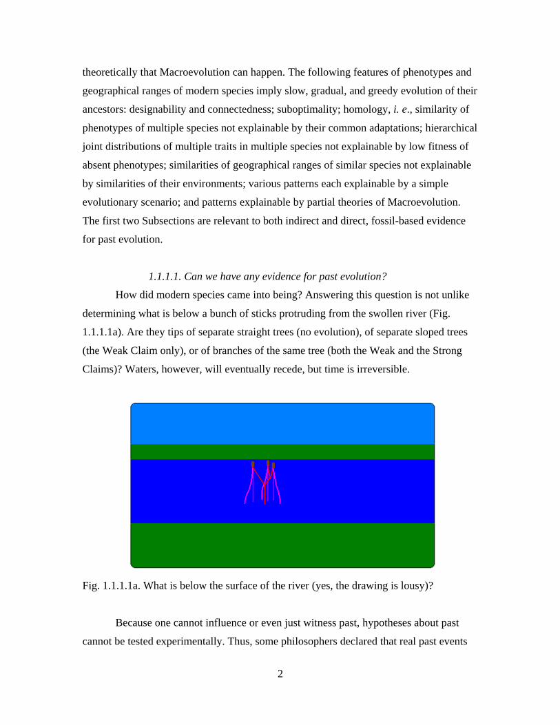
How did modern species came into being? Answering this question is not unlike

determining what is below a bunch of sticks protruding from the swollen river (Fig.

1.1.1.1a). Are they tips of separate straight trees (no evolution), of separate sloped trees

(the Weak Claim only), or of branches of the same tree (both the Weak and the Strong

Claims)? Waters, however, will eventually recede, but time is irreversible.

Fig. 1.1.1.1a. What is below the surface of the river (yes, the drawing is lousy)?

Because one cannot influence or even just witness past, hypotheses about past

cannot be tested experimentally. Thus, some philosophers declared that real past events

3

can never be discovered, so that cosmology or evolutionary biology are not natural

sciences. Indeed, studying past readily opens a can of philosophical worms. Can we rule

out that the Earth, with all the innumerable traces of its long history (and of ancient

civilizations), somehow appeared suddenly only 10000 (or even just 1000) years ago? Is

present really more accessible to investigation than past? We experience only our

sensations, so is there any present Reality behind them? What is time?

However, let us render philosophy unto philosophers (until Chapter 4.2) and

accept a naive belief that there is, and was, for some time, the real Material Universe

outside us. If you disagree, stop imagining that you are reading this text right now.

Moreover, we need to believe that this Universe is not entirely chaotic or absolutely free

to do anything it wishes, but, instead, is governed by certain laws of nature, whatever

their origin might be, and, thus, is amenable to scientific investigation.

Laws of nature can be thought of as restrictions on what could possibly happen.

Some of them are rigid, so that the corresponding aspects of the future can be predicted

exactly. For example, the energy of a closed system will always remain the same. Other

laws of nature are stochastic: it is impossible to predict, for example, when a particular

atom of 14

C will decay. Still, some events, such as simultaneous decay of all 14

C atoms

within a macroscopic sample, are so improbable that we can safely regard them as

impossible. Phenomena which obey laws of nature are called natural, as opposed to

"supernatural" miracles, not bound by any natural restrictions (there is no need to debate

here if miracles ever happen).

Studying past is based on yet another belief, called uniformitarianism, that laws of

nature remained more or less invariant over a long time. Uniformitarianism implies, for

example, that an object we call "a fossilized Tyrannosaurus rex skeleton" is, indeed, a

remnant of a huge animal with impressive teeth, now apparently extinct (of course, this

fact in itself does not prove evolution). Skeletons do not naturally condense from rocks

these days, and we accept that this never happened. If so, present can be the key to past, a

premise developed in 1830 by Charles Lyell in his book "Principles of Geology", and we

may be able to deduce past from contemporary theory, patterns, and data. This approach

can work in several ways.

First, at some moment in the past, an object could "freeze", i. e., more or less stop

changing. Then, when we unearth it (often, literally), we receive a message from the past.

4

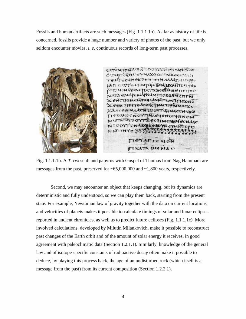
Fossils and human artifacts are such messages (Fig. 1.1.1.1b). As far as history of life is

concerned, fossils provide a huge number and variety of photos of the past, but we only

seldom encounter movies, i. e. continuous records of long-term past processes.

Fig. 1.1.1.1b. A T. rex scull and papyrus with Gospel of Thomas from Nag Hammadi are

messages from the past, preserved for ~65,000,000 and ~1,800 years, respectively.

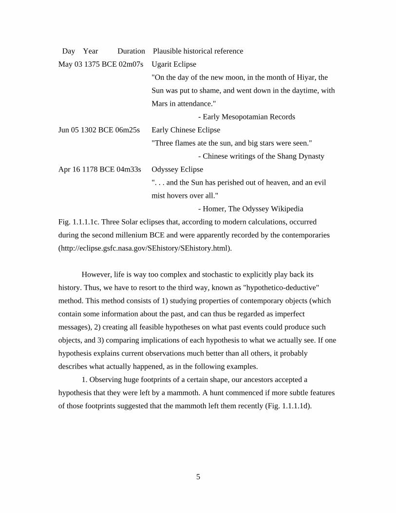
Second, we may encounter an object that keeps changing, but its dynamics are

deterministic and fully understood, so we can play them back, starting from the present

state. For example, Newtonian law of gravity together with the data on current locations

and velocities of planets makes it possible to calculate timings of solar and lunar eclipses

reported in ancient chronicles, as well as to predict future eclipses (Fig. 1.1.1.1c). More

involved calculations, developed by Milutin Milankovich, make it possible to reconstruct

past changes of the Earth orbit and of the amount of solar energy it receives, in good

agreement with paleoclimatic data (Section 1.2.1.1). Similarly, knowledge of the general

law and of isotope-specific constants of radioactive decay often make it possible to

deduce, by playing this process back, the age of an undisturbed rock (which itself is a

message from the past) from its current composition (Section 1.2.2.1).

5

Day Year Duration Plausible historical reference

May 03 1375 BCE 02m07s Ugarit Eclipse

"On the day of the new moon, in the month of Hiyar, the

Sun was put to shame, and went down in the daytime, with

Mars in attendance."

- Early Mesopotamian Records

Jun 05 1302 BCE 06m25s Early Chinese Eclipse

"Three flames ate the sun, and big stars were seen."

- Chinese writings of the Shang Dynasty

Apr 16 1178 BCE 04m33s Odyssey Eclipse

". . . and the Sun has perished out of heaven, and an evil

mist hovers over all."

- Homer, The Odyssey Wikipedia

Fig. 1.1.1.1c. Three Solar eclipses that, according to modern calculations, occurred

during the second millenium BCE and were apparently recorded by the contemporaries

(http://eclipse.gsfc.nasa.gov/SEhistory/SEhistory.html).

However, life is way too complex and stochastic to explicitly play back its

history. Thus, we have to resort to the third way, known as "hypothetico-deductive"

method. This method consists of 1) studying properties of contemporary objects (which

contain some information about the past, and can thus be regarded as imperfect

messages), 2) creating all feasible hypotheses on what past events could produce such

objects, and 3) comparing implications of each hypothesis to what we actually see. If one

hypothesis explains current observations much better than all others, it probably

describes what actually happened, as in the following examples.

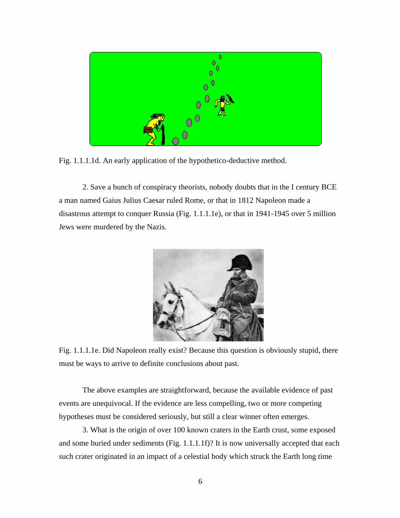
1. Observing huge footprints of a certain shape, our ancestors accepted a

hypothesis that they were left by a mammoth. A hunt commenced if more subtle features

of those footprints suggested that the mammoth left them recently (Fig. 1.1.1.1d).

6

Fig. 1.1.1.1d. An early application of the hypothetico-deductive method.

2. Save a bunch of conspiracy theorists, nobody doubts that in the I century BCE

a man named Gaius Julius Caesar ruled Rome, or that in 1812 Napoleon made a

disastrous attempt to conquer Russia (Fig. 1.1.1.1e), or that in 1941-1945 over 5 million

Jews were murdered by the Nazis.

Fig. 1.1.1.1e. Did Napoleon really exist? Because this question is obviously stupid, there

must be ways to arrive to definite conclusions about past.

The above examples are straightforward, because the available evidence of past

events are unequivocal. If the evidence are less compelling, two or more competing

hypotheses must be considered seriously, but still a clear winner often emerges.

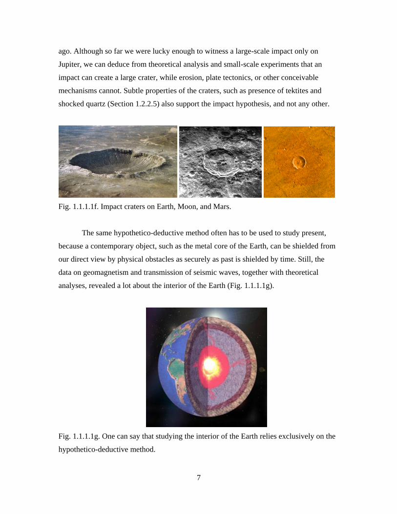
3. What is the origin of over 100 known craters in the Earth crust, some exposed

and some buried under sediments (Fig. 1.1.1.1f)? It is now universally accepted that each

such crater originated in an impact of a celestial body which struck the Earth long time

7

ago. Although so far we were lucky enough to witness a large-scale impact only on

Jupiter, we can deduce from theoretical analysis and small-scale experiments that an

impact can create a large crater, while erosion, plate tectonics, or other conceivable

mechanisms cannot. Subtle properties of the craters, such as presence of tektites and

shocked quartz (Section 1.2.2.5) also support the impact hypothesis, and not any other.

Fig. 1.1.1.1f. Impact craters on Earth, Moon, and Mars.

The same hypothetico-deductive method often has to be used to study present,

because a contemporary object, such as the metal core of the Earth, can be shielded from

our direct view by physical obstacles as securely as past is shielded by time. Still, the

data on geomagnetism and transmission of seismic waves, together with theoretical

analyses, revealed a lot about the interior of the Earth (Fig. 1.1.1.1g).

Fig. 1.1.1.1g. One can say that studying the interior of the Earth relies exclusively on the

hypothetico-deductive method.

8

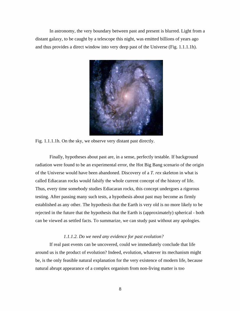
In astronomy, the very boundary between past and present is blurred. Light from a

distant galaxy, to be caught by a telescope this night, was emitted billions of years ago

and thus provides a direct window into very deep past of the Universe (Fig. 1.1.1.1h).

Fig. 1.1.1.1h. On the sky, we observe very distant past directly.

Finally, hypotheses about past are, in a sense, perfectly testable. If background

radiation were found to be an experimental error, the Hot Big Bang scenario of the origin

of the Universe would have been abandoned. Discovery of a T. rex skeleton in what is

called Ediacaran rocks would falsify the whole current concept of the history of life.

Thus, every time somebody studies Ediacaran rocks, this concept undergoes a rigorous

testing. After passing many such tests, a hypothesis about past may become as firmly

established as any other. The hypothesis that the Earth is very old is no more likely to be

rejected in the future that the hypothesis that the Earth is (approximately) spherical - both

can be viewed as settled facts. To summarize, we can study past without any apologies.

1.1.1.2. Do we need any evidence for past evolution?

If real past events can be uncovered, could we immediately conclude that life

around us is the product of evolution? Indeed, evolution, whatever its mechanism might

be, is the only feasible natural explanation for the very existence of modern life, because

natural abrupt appearance of a complex organism from non-living matter is too

9

improbable (Fig 1.1.1.2a). Thus, to deny evolution, one must assume a direct intervention

of a supernatural power.

Fig. 1.1.1.2a. The birth of Aphrodite from sea waves.

Of course, modern studies of the Universe avoid invoking such interventions.

These days, nobody would claim that T. rex skeletons appeared miraculously. A person

who attributes AIDS to improper alignment of planets must not practice medicine. And

if, God forbid, you will be accused of shooting somebody, do not try to claim that the

fatal shot had been fired by an evil spirit (Fig 1.1.1.2b). One is free to believe that

somebody contracted AIDS, while many others did not, as a punishment for his sins, or

as a means of testing his faith, but the immediate cause of the disease is always infection

with HIV. A scientist, a doctor, or a detective always looks for at least proximal natural

explanations of their facts, and so far this approach worked very well. As a result, the

existence of a natural explanation of any fact is routinely treated as null-hypothesis,

accepted by default, as long as all natural explanations cannot be ruled out.

10

Fig. 1.1.1.2a. A hopeless criminal defense.

Moreover, admitting a supernatural intervention may violate a basic scientific

tenet, known as Occam's razor: to explain your facts, use only the minimal necessary set

of fundamental principles, and do not invoke extra ones. "Sire, I have no need for that

hypothesis" - Laplace replied famously, when Napoleon asked him about the place for

God in his Celestial Mechanics. Because we know that gravity can keep planets on their

orbits, an organism can grow its skeleton, HIV can cause AIDS, and a human can fire a

gun, supernatural explanations of the corresponding facts are redundant.

However, the situation is different for "if not evolution, what else?" argument,

because currently it is impossible to prove that gradual origin of primitive life from non-

living matter, followed by Macroevolution, can naturally produce modern life. Profound

changes of lineages have not been observed directly, and available theory is too weak for

any firm conclusions, either positive or negative. Thus, Occam's razor does not force us

to accept natural, evolutionary origin of life around us.

Even to accept past evolution just as an unrejected natural explanation is perhaps

too reckless. To be sure, some conclusions of utmost importance are based on our

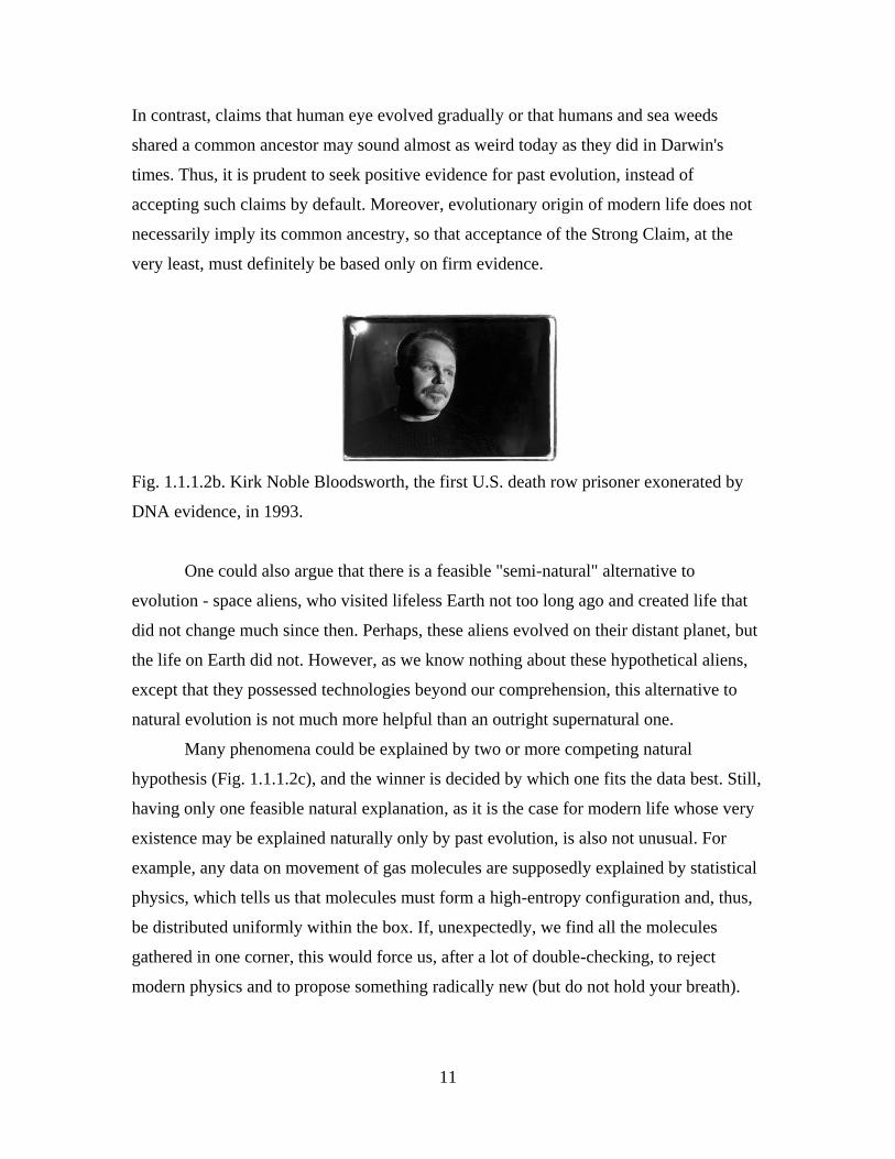
willingness to dismiss the very possibility of a supernatural explanation. Many

individuals, each found guilty "beyond reasonable doubt", were acquitted when DNA

evidence exonerated them (Fig. 1.1.1.2b), and no sane person ever argued that a

mismatch between the DNA sequences from the crime scene and from the convicted

person could be due to a miracle. However, there is a simple natural explanation for such

a mismatch: the conviction was wrong, and the crime was committed by somebody else.

11

In contrast, claims that human eye evolved gradually or that humans and sea weeds

shared a common ancestor may sound almost as weird today as they did in Darwin's

times. Thus, it is prudent to seek positive evidence for past evolution, instead of

accepting such claims by default. Moreover, evolutionary origin of modern life does not

necessarily imply its common ancestry, so that acceptance of the Strong Claim, at the

very least, must definitely be based only on firm evidence.

Fig. 1.1.1.2b. Kirk Noble Bloodsworth, the first U.S. death row prisoner exonerated by

DNA evidence, in 1993.

One could also argue that there is a feasible "semi-natural" alternative to

evolution - space aliens, who visited lifeless Earth not too long ago and created life that

did not change much since then. Perhaps, these aliens evolved on their distant planet, but

the life on Earth did not. However, as we know nothing about these hypothetical aliens,

except that they possessed technologies beyond our comprehension, this alternative to

natural evolution is not much more helpful than an outright supernatural one.

Many phenomena could be explained by two or more competing natural

hypothesis (Fig. 1.1.1.2c), and the winner is decided by which one fits the data best. Still,

having only one feasible natural explanation, as it is the case for modern life whose very

existence may be explained naturally only by past evolution, is also not unusual. For

example, any data on movement of gas molecules are supposedly explained by statistical

physics, which tells us that molecules must form a high-entropy configuration and, thus,

be distributed uniformly within the box. If, unexpectedly, we find all the molecules

gathered in one corner, this would force us, after a lot of double-checking, to reject

modern physics and to propose something radically new (but do not hold your breath).

12

Fig. 1.1.1.2c. Competing natural hypotheses.

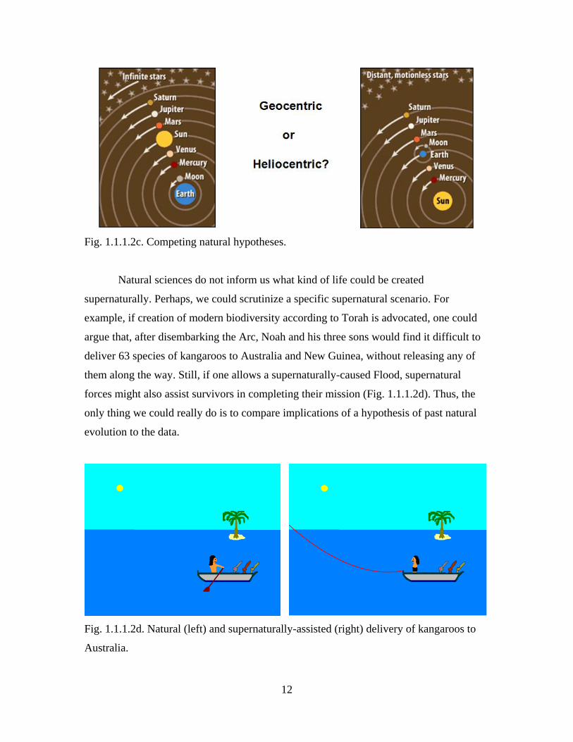
Natural sciences do not inform us what kind of life could be created

supernaturally. Perhaps, we could scrutinize a specific supernatural scenario. For

example, if creation of modern biodiversity according to Torah is advocated, one could

argue that, after disembarking the Arc, Noah and his three sons would find it difficult to

deliver 63 species of kangaroos to Australia and New Guinea, without releasing any of

them along the way. Still, if one allows a supernaturally-caused Flood, supernatural

forces might also assist survivors in completing their mission (Fig. 1.1.1.2d). Thus, the

only thing we could really do is to compare implications of a hypothesis of past natural

evolution to the data.

Fig. 1.1.1.2d. Natural (left) and supernaturally-assisted (right) delivery of kangaroos to

Australia.

13

So, what do we expect to see in modern life if it is a product of natural evolution?

Are there any reasons to conclude that a) ancestors of modern species were different from

them and b) multiple modern species shared common ancestors? Careful dissection of

indirect evidence for past evolution provides a natural point of departure for studying

evolutionary biology, as well as for dealing with creationism and related pseudoscience.

1.1.1.3. Designability and connectedness

If living beings changed in the succession of generations, these changes were

gradual and slow. Indeed, a naturally produced daughter must be similar to her mother,

and low rates of evolution (if any) is an empirical fact: in the course of a small number of

generations species do not change too much. Thus, evolutionary origin of modern species

can affect their phenotypes, and an indirect evidence for past evolution can emerge if two

complementary conditions are met: 1) there is a discrepancy between phenotypes of

modern species and what can be expected if we take into account only the current

environments and fitness landscapes and 2) these phenotypes are consistent with the

hypothesis of their evolutionary origin. In other words, if phenotypes of all modern

species were fully explainable by their adaptations to the current environments, we would

not possess any indirect evidence for past evolution.

If modern species are products of gradual evolution, they must meet two "global"

tests:

1) The genome and the phenotype of a modern species must be designable - there

must exist a continuum of fit genotypes connecting it with some very simple genotypes

which could have originated from non-living matter - otherwise, the Weak Claim cannot

be true for this species. In Darwin's words, "If it could be demonstrated that any complex

organ existed which could not possibly have been formed by numerous, successive, slight

modifications, my theory would absolutely break down".

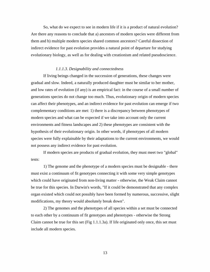
2) The genomes and the phenotypes of all species within a set must be connected

to each other by a continuum of fit genotypes and phenotypes - otherwise the Strong

Claim cannot be true for this set (Fig 1.1.1.3a). If life originated only once, this set must

include all modern species.

14

Fig. 1.1.1.3a. Past evolution implies designability and connectedness of modern species.

Designability and connectedness of modern species depend on the global fitness

landscape. They would provide very powerful evidence for evolution, because a priori

there is no reason for any complex entity to possess such properties. However, we cannot

currently say much on this subject: global features of fitness landscapes are mostly

unknown, and empirically we know almost nothing about designability of modern

species and just a little about their connectedness (Fig. I36). Thus, less ambitious tests of

the evolutionary origin of modern life, not requiring comprehensive knowledge of fitness

landscapes, are needed.

1.1.1.4. Suboptimality

Such less ambitious tests rely only on local properties of the fitness landscape, in

particular, on how genotypes and phenotypes of modern species are located on it. Let us

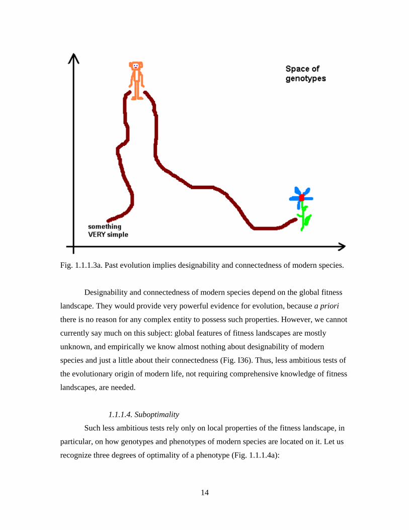
recognize three degrees of optimality of a phenotype (Fig. 1.1.1.4a):

15

I) Suboptimality: a phenotype is located clearly below the highest peak on the

fitness landscape, i. e. its fitness is well below the global maximum.

II) Non-unique optimality: a phenotype is located more or less at the same level

as the highest peak, i. e. it possesses a near-maximal fitness, together with other

phenotype(s). We will regard a phenotype as non-uniquely optimal if we cannot prove

that it is suboptimal, but are reasonably sure that there are other at least equally fit

phenotypes.

III) Unique optimality: a phenotype is located at the highest peak, i. e. it alone

possesses the maximal fitness.

Fig. 1.1.1.4a. Suboptimal (a), non-uniquely optimal (b), and uniquely optimal (c)

phenotypes are shown by red dots.

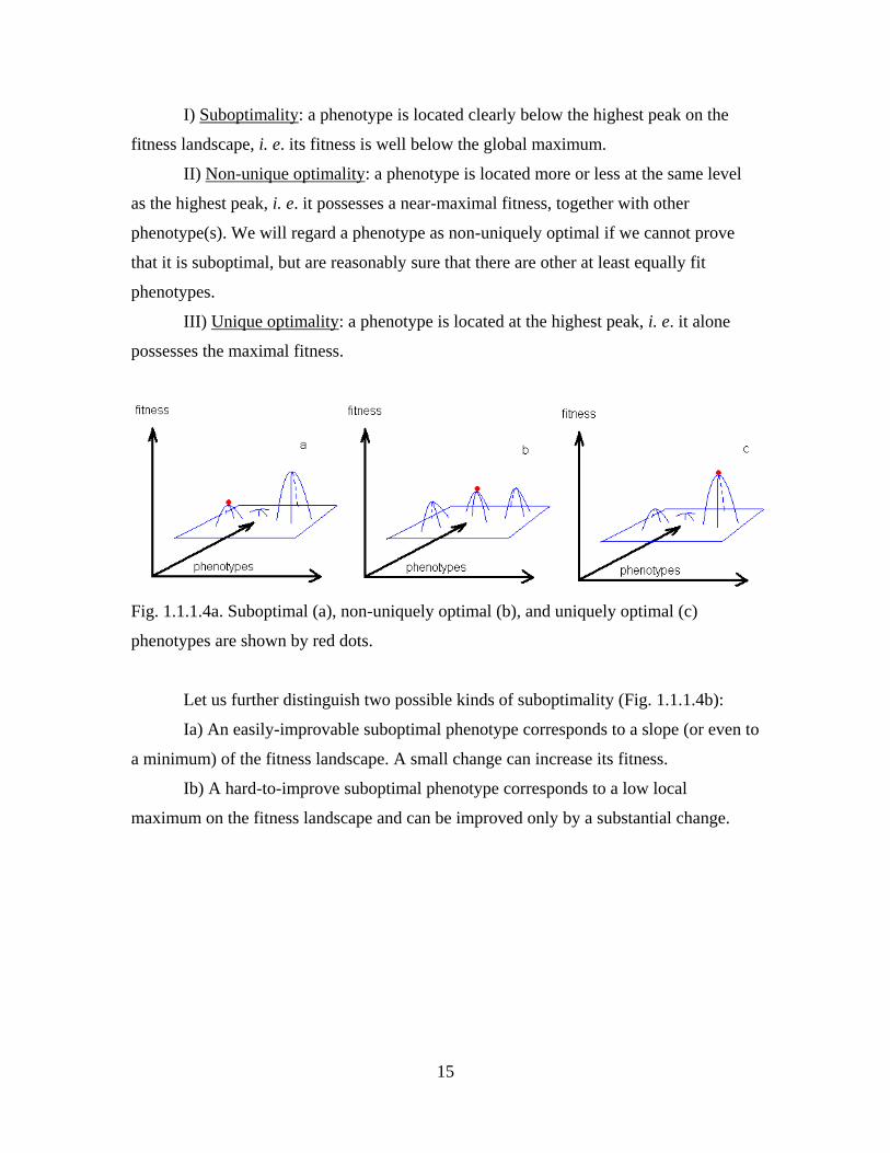
Let us further distinguish two possible kinds of suboptimality (Fig. 1.1.1.4b):

Ia) An easily-improvable suboptimal phenotype corresponds to a slope (or even to

a minimum) of the fitness landscape. A small change can increase its fitness.

Ib) A hard-to-improve suboptimal phenotype corresponds to a low local

maximum on the fitness landscape and can be improved only by a substantial change.

16

Fig. 1.1.1.4b. Easily-improvable (a) and a hard-to-improve (b) suboptimal phenotypes.

We will usually assume that evolution, if any, is not only gradual and slow but

also greedy, in a sense that a lineage changes in the direction that maximized fitness

under its current conditions. Assumption of greedy evolution is reasonable because

natural selection relies only on variation that is currently present and it is hard to imagine

any other natural mechanism for adaptive evolution, especially one that could have any

foresight (Fig. I22).

Gradual, slow evolution will produce easily-improvable suboptimal phenotypes if

there was not enough time for an evolving lineage to reach a fitness peak, perhaps

because the environment and the fitness landscape changed recently. Evolution that was

also greedy may produce hard-to-improve suboptimal phenotypes even when provided

with unlimited time. Indeed, for such evolution any fitness peak represents a trap, as a

lineage which initially belonged to its domain of attraction will reach this peak and

remain on it, as long as the peak persists, regardless of whether there are any higher

peaks (Fig. I25).

Thus, if the phenotype of a species is suboptimal, this is an indirect evidence for

the Weak Claim for this species, because evolution, if it happened, must be prone to

producing suboptimal phenotypes. A phenotype located at the top of a low peak suggests

an evolutionary trajectory of the ancestral lineage that started within the domain of

attraction of this peak a long time ago. A phenotype located at the slope of a peak

suggests that evolution is still ongoing.

17

Evidence for past evolution emerges only if a modern species has an

unconditionally suboptimal phenotype, imperfect under any feasible environment.

Indeed, well-developed eyes of some animals found in caves, while clearly suboptimal

under darkness, are useful on the surface and, thus, do not imply evolution, but only

recent colonization of caves. Similarly, when a polar bear suffers from the heat in

Washington, DC zoo, this is not an evidence for its suboptimality and evolution.

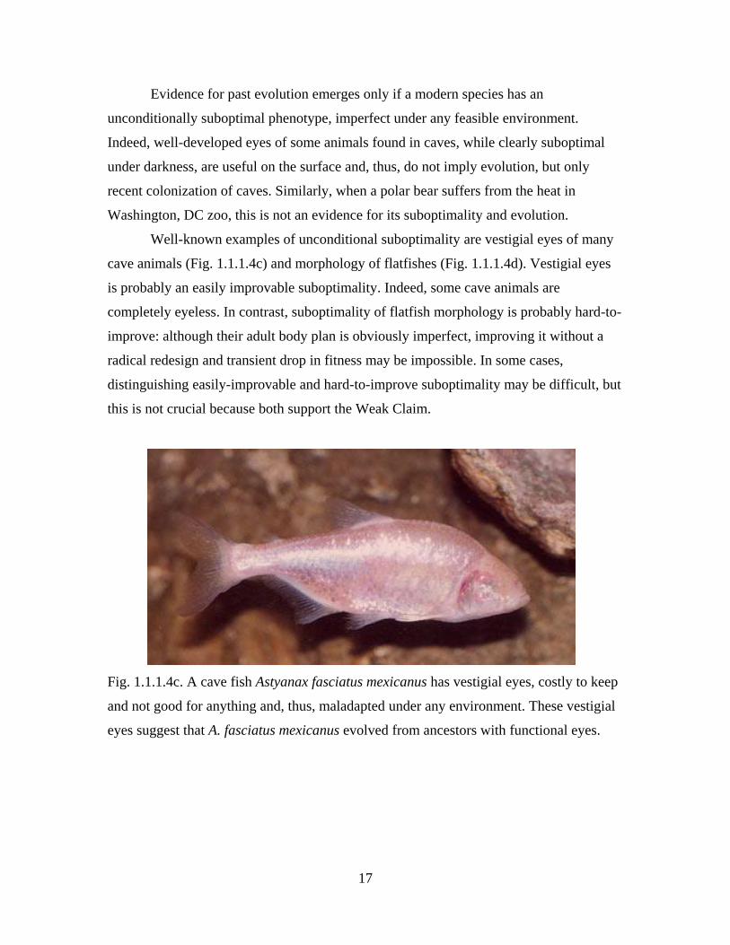
Well-known examples of unconditional suboptimality are vestigial eyes of many

cave animals (Fig. 1.1.1.4c) and morphology of flatfishes (Fig. 1.1.1.4d). Vestigial eyes

is probably an easily improvable suboptimality. Indeed, some cave animals are

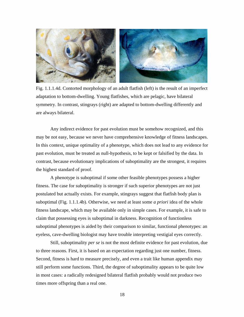
completely eyeless. In contrast, suboptimality of flatfish morphology is probably hard-to-

improve: although their adult body plan is obviously imperfect, improving it without a

radical redesign and transient drop in fitness may be impossible. In some cases,

distinguishing easily-improvable and hard-to-improve suboptimality may be difficult, but

this is not crucial because both support the Weak Claim.

Fig. 1.1.1.4c. A cave fish Astyanax fasciatus mexicanus has vestigial eyes, costly to keep

and not good for anything and, thus, maladapted under any environment. These vestigial

eyes suggest that A. fasciatus mexicanus evolved from ancestors with functional eyes.

18

Fig. 1.1.1.4d. Contorted morphology of an adult flatfish (left) is the result of an imperfect

adaptation to bottom-dwelling. Young flatfishes, which are pelagic, have bilateral

symmetry. In contrast, stingrays (right) are adapted to bottom-dwelling differently and

are always bilateral.

Any indirect evidence for past evolution must be somehow recognized, and this

may be not easy, because we never have comprehensive knowledge of fitness landscapes.

In this context, unique optimality of a phenotype, which does not lead to any evidence for

past evolution, must be treated as null-hypothesis, to be kept or falsified by the data. In

contrast, because evolutionary implications of suboptimality are the strongest, it requires

the highest standard of proof.

A phenotype is suboptimal if some other feasible phenotypes possess a higher

fitness. The case for suboptimality is stronger if such superior phenotypes are not just

postulated but actually exists. For example, stingrays suggest that flatfish body plan is

suboptimal (Fig. 1.1.1.4b). Otherwise, we need at least some a priori idea of the whole

fitness landscape, which may be available only in simple cases. For example, it is safe to

claim that possessing eyes is suboptimal in darkness. Recognition of functionless

suboptimal phenotypes is aided by their comparison to similar, functional phenotypes: an

eyeless, cave-dwelling biologist may have trouble interpreting vestigial eyes correctly.

Still, suboptimality per se is not the most definite evidence for past evolution, due

to three reasons. First, it is based on an expectation regarding just one number, fitness.

Second, fitness is hard to measure precisely, and even a trait like human appendix may

still perform some functions. Third, the degree of suboptimality appears to be quite low

in most cases: a radically redesigned bilateral flatfish probably would not produce two

times more offspring than a real one.

19

In contrast to suboptimality, optimality of a modern species does not per se

provide any support for the Weak Claim for its lineage. An optimal phenotype does not

contradict past evolution, as long as it designable, but it does not offer any evidence for

the ancestors of a modern species being different from it. This is the case both for perfect

general-purpose adaptations and for perfect adaptations restricted to very specific

environments. For example, sharks, ichthyosaurs, and whales all have similar body

shapes (Fig. I27), dictated by the general laws of hydrodynamics and fit for any active

swimmer. In contrast, mimicry is a specific adaptation to the presence of unpalatable

organisms with a particular coloration (Fig. I18). Although mimicry can be comfortably

explained by natural selection, it does not immediately supply any evidence for past

evolution. The same, of course, is also true for streamlined body shapes or any other

adaptation.

This conclusion may look paradoxical: Darwinian evolution is driven by natural

selection which strives to improve adaptation, and one may think that perfect adaptations

of modern species offer the best indirect evidence for evolution by natural selection of

their ancestors. However, exactly the opposite is true! At least three reasons are behind

this paradox. First, gradual, slow, and greedy evolution must be prone of producing

suboptimal phenotypes. Second, modern species must be adapted just in order to survive.

Thus, perfect adaptations are in accord with our expectations, regardless of any possible

past evolution. Finally, as we have no natural alternative to evolution, evidence for it

cannot emerge from something that evolution could achieve but its alternative could not.

Instead, past evolution may be revealed only by what it could not achieve, and, far from

being omnipotent, it could hardly produce perfect adaptations in all cases.

1.1.1.5. Unforced similarity, or homology

The most important among indirect evidence for past evolution are similarities

between modern phenotypes not explainable by their common adaptations. Two

millennia before Darwin, a Latin poet Quintus Ennius (239–169 BCE) exclaimed: "Simia

quam similis turpissima bestia nobis" (The monkey, how similar that most ugly beast is

to us!). However, this observation did not lead to immediate recognition of the common

ancestry of humans and monkeys, and for a good reason, because not every similarity

between modern species supports the Strong Claim for them. One must be sure that this

20

similarity is not forced, i. e. does not reflect a uniquely optimal adaptation. Thus, there is

no reason to believe that sharks, ichthyosaurs, and whales inherited their similar body

shapes (Fig. I27) from their common ancestor (they did not).

Instead, evidence for the Strong Claim for a set of modern species appears only if

they all share the same suboptimal, or at least a non-uniquely optimal, phenotype. Indeed,

slow, gradual, and greedy evolution must be prone to preserve common ancestral

properties in diverging species, even when these properties are not uniquely optimal, and,

thus, sharing them is not forced by common adaptation. To refer to such unforced

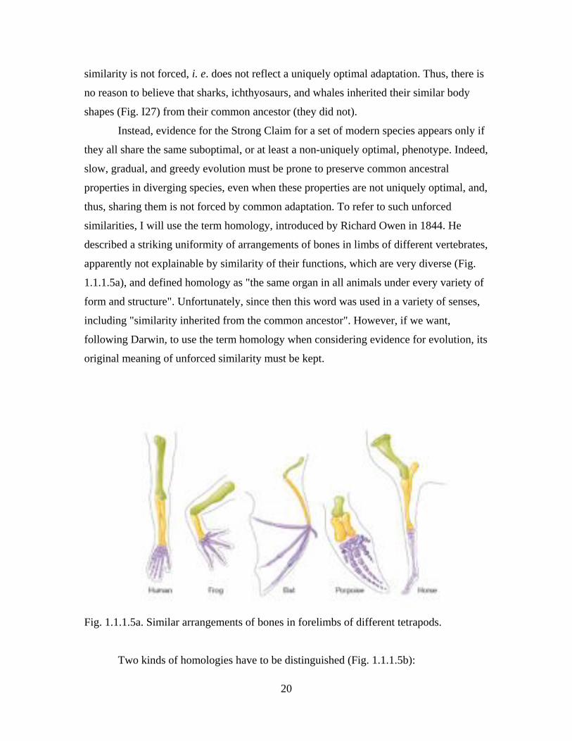
similarities, I will use the term homology, introduced by Richard Owen in 1844. He

described a striking uniformity of arrangements of bones in limbs of different vertebrates,

apparently not explainable by similarity of their functions, which are very diverse (Fig.

1.1.1.5a), and defined homology as "the same organ in all animals under every variety of

form and structure". Unfortunately, since then this word was used in a variety of senses,

including "similarity inherited from the common ancestor". However, if we want,

following Darwin, to use the term homology when considering evidence for evolution, its

original meaning of unforced similarity must be kept.

Fig. 1.1.1.5a. Similar arrangements of bones in forelimbs of different tetrapods.

Two kinds of homologies have to be distinguished (Fig. 1.1.1.5b):

21

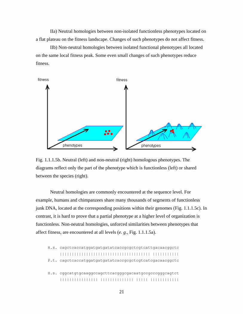
IIa) Neutral homologies between non-isolated functionless phenotypes located on

a flat plateau on the fitness landscape. Changes of such phenotypes do not affect fitness.

IIb) Non-neutral homologies between isolated functional phenotypes all located

on the same local fitness peak. Some even small changes of such phenotypes reduce

fitness.

Fig. 1.1.1.5b. Neutral (left) and non-neutral (right) homologous phenotypes. The

diagrams reflect only the part of the phenotype which is functionless (left) or shared

between the species (right).

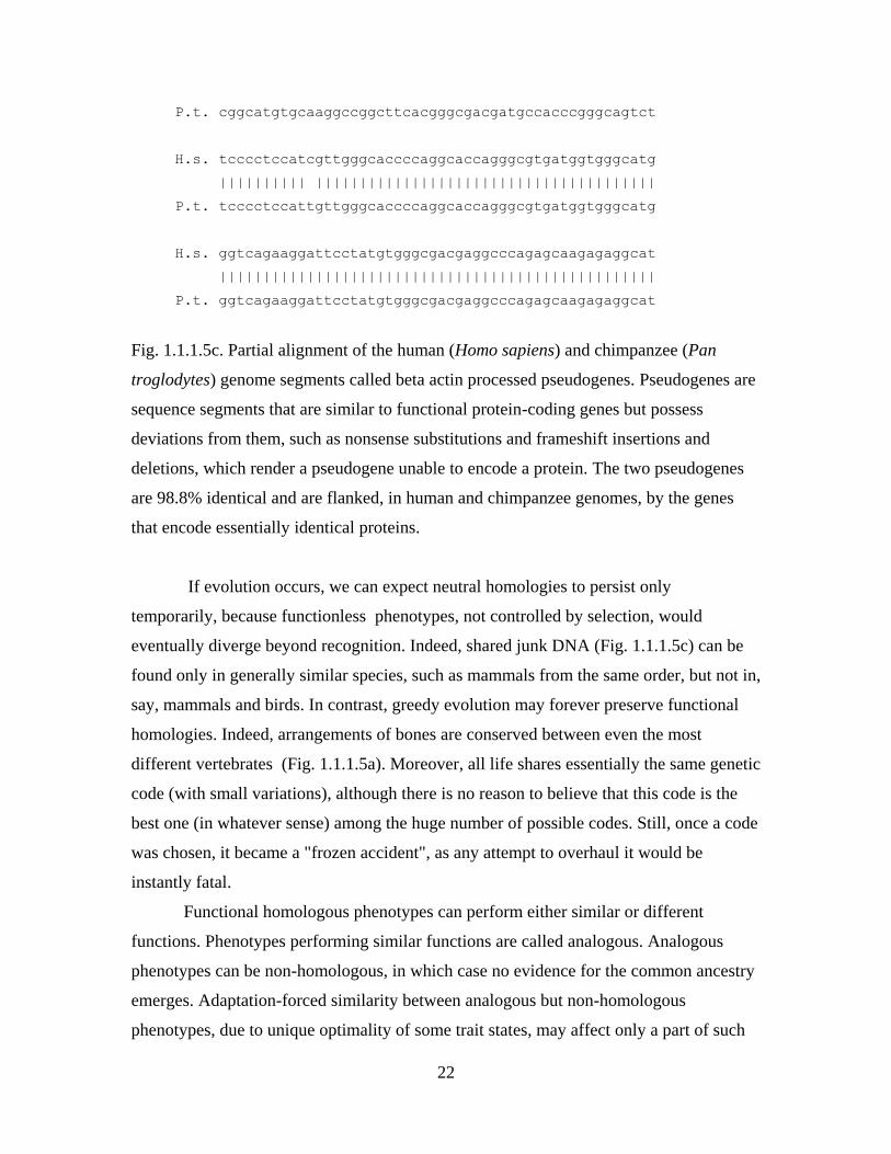
Neutral homologies are commonly encountered at the sequence level. For

example, humans and chimpanzees share many thousands of segments of functionless

junk DNA, located at the corresponding positions within their genomes (Fig. 1.1.1.5c). In

contrast, it is hard to prove that a partial phenotype at a higher level of organization is

functionless. Non-neutral homologies, unforced similarities between phenotypes that

affect fitness, are encountered at all levels (e. g., Fig. 1.1.1.5a).

H.s. cagctcaccatggatgatgatatcaccgcgctcgtcattgacaacggctc

|||||||||||||||||||||||||||||||||||||| |||||||||||

P.t. cagctcaccatggatgatgatatcaccgcgctcgtcatcgacaacggctc

H.s. cggcatgtgcaaggccagcttcacgggcgacaatgccgcccgggcagtct

|||||||||||||||| |||||||||||||| ||||| ||||||||||||

22

P.t. cggcatgtgcaaggccggcttcacgggcgacgatgccacccgggcagtct

H.s. tcccctccatcgttgggcaccccaggcaccagggcgtgatggtgggcatg

|||||||||| |||||||||||||||||||||||||||||||||||||||

P.t. tcccctccattgttgggcaccccaggcaccagggcgtgatggtgggcatg

H.s. ggtcagaaggattcctatgtgggcgacgaggcccagagcaagagaggcat

||||||||||||||||||||||||||||||||||||||||||||||||||

P.t. ggtcagaaggattcctatgtgggcgacgaggcccagagcaagagaggcat

Fig. 1.1.1.5c. Partial alignment of the human (Homo sapiens) and chimpanzee (Pan

troglodytes) genome segments called beta actin processed pseudogenes. Pseudogenes are

sequence segments that are similar to functional protein-coding genes but possess

deviations from them, such as nonsense substitutions and frameshift insertions and

deletions, which render a pseudogene unable to encode a protein. The two pseudogenes

are 98.8% identical and are flanked, in human and chimpanzee genomes, by the genes

that encode essentially identical proteins.

If evolution occurs, we can expect neutral homologies to persist only

temporarily, because functionless phenotypes, not controlled by selection, would

eventually diverge beyond recognition. Indeed, shared junk DNA (Fig. 1.1.1.5c) can be

found only in generally similar species, such as mammals from the same order, but not in,

say, mammals and birds. In contrast, greedy evolution may forever preserve functional

homologies. Indeed, arrangements of bones are conserved between even the most

different vertebrates (Fig. 1.1.1.5a). Moreover, all life shares essentially the same genetic

code (with small variations), although there is no reason to believe that this code is the

best one (in whatever sense) among the huge number of possible codes. Still, once a code

was chosen, it became a "frozen accident", as any attempt to overhaul it would be

instantly fatal.

Functional homologous phenotypes can perform either similar or different

functions. Phenotypes performing similar functions are called analogous. Analogous

phenotypes can be non-homologous, in which case no evidence for the common ancestry

emerges. Adaptation-forced similarity between analogous but non-homologous

phenotypes, due to unique optimality of some trait states, may affect only a part of such

23

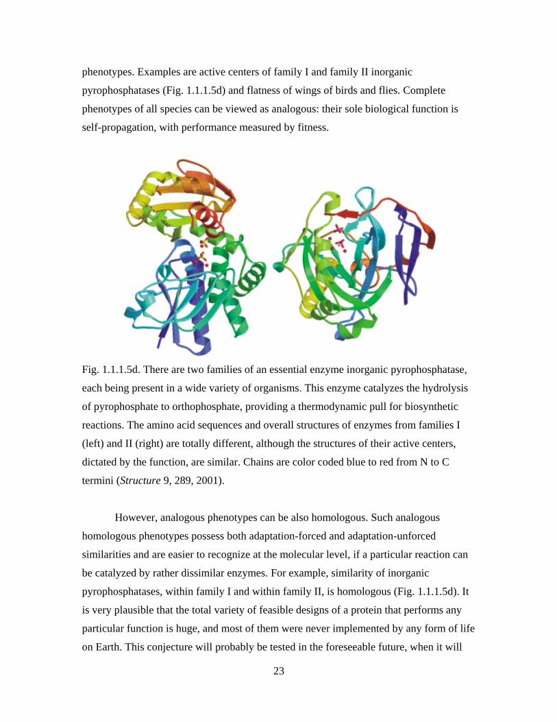
phenotypes. Examples are active centers of family I and family II inorganic

pyrophosphatases (Fig. 1.1.1.5d) and flatness of wings of birds and flies. Complete

phenotypes of all species can be viewed as analogous: their sole biological function is

self-propagation, with performance measured by fitness.

Fig. 1.1.1.5d. There are two families of an essential enzyme inorganic pyrophosphatase,

each being present in a wide variety of organisms. This enzyme catalyzes the hydrolysis

of pyrophosphate to orthophosphate, providing a thermodynamic pull for biosynthetic

reactions. The amino acid sequences and overall structures of enzymes from families I

(left) and II (right) are totally different, although the structures of their active centers,

dictated by the function, are similar. Chains are color coded blue to red from N to C

termini (Structure 9, 289, 2001).

However, analogous phenotypes can be also homologous. Such analogous

homologous phenotypes possess both adaptation-forced and adaptation-unforced

similarities and are easier to recognize at the molecular level, if a particular reaction can

be catalyzed by rather dissimilar enzymes. For example, similarity of inorganic

pyrophosphatases, within family I and within family II, is homologous (Fig. 1.1.1.5d). It

is very plausible that the total variety of feasible designs of a protein that performs any

particular function is huge, and most of them were never implemented by any form of life

on Earth. This conjecture will probably be tested in the foreseeable future, when it will

24

become possible to create novel proteins performing desired functions. Similarly, there is

little doubt that similarity of the arrangement of bones within wings of birds and bats

goes beyond what is necessary for flight, but a definite proof of this claim may be far

away. In effect, to claim that similarity between analogous phenotypes is homologous is

to claim that many other ways are possible for performing their function (if any) or, in

other words, that there are many other, perhaps mostly empty, high regions on the fitness

landscape. Apparently, this is a rule at all levels of organization, and unique optimal

solutions exist only when they are dictated by some basic laws of nature (Fig. I26;

hexagonal honeycomb is optimal geometrically, etc.).

Still, homology is most salient when it involves non-analogous phenotypes that

perform substantially different functions, such as human hands, bat wings, and dolphin

flippers (Fig. 1.1.1.5a), or no function at all, such as pseudogenes of different species

(Fig. 1.1.1.5c). Indeed, all similarities between non-analogous phenotypes must be

homologous.

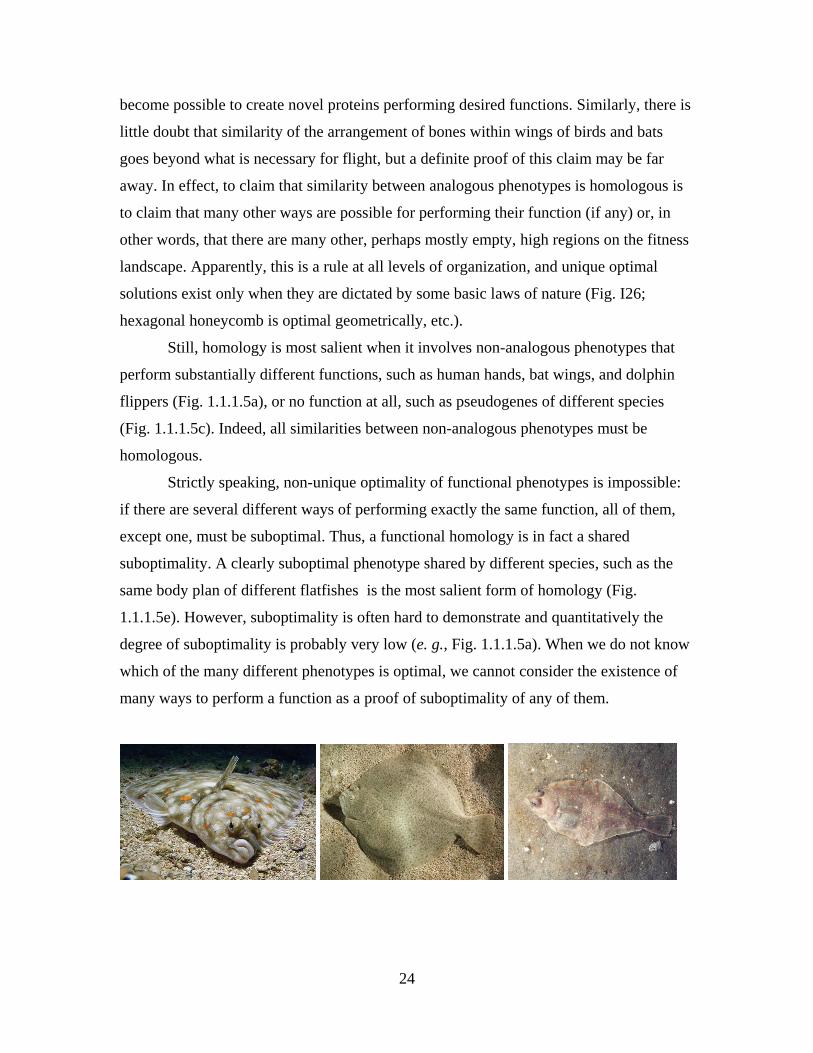
Strictly speaking, non-unique optimality of functional phenotypes is impossible:

if there are several different ways of performing exactly the same function, all of them,

except one, must be suboptimal. Thus, a functional homology is in fact a shared

suboptimality. A clearly suboptimal phenotype shared by different species, such as the

same body plan of different flatfishes is the most salient form of homology (Fig.

1.1.1.5e). However, suboptimality is often hard to demonstrate and quantitatively the

degree of suboptimality is probably very low (e. g., Fig. 1.1.1.5a). When we do not know

which of the many different phenotypes is optimal, we cannot consider the existence of

many ways to perform a function as a proof of suboptimality of any of them.

25

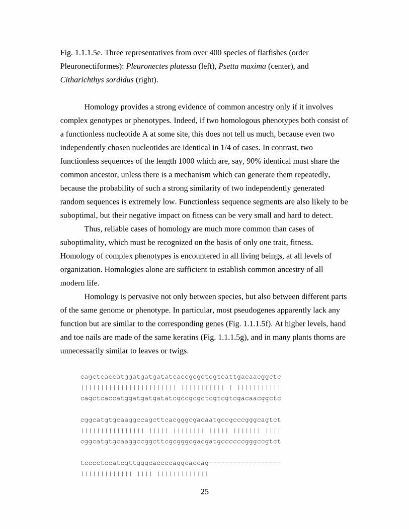
Fig. 1.1.1.5e. Three representatives from over 400 species of flatfishes (order

Pleuronectiformes): Pleuronectes platessa (left), Psetta maxima (center), and

Citharichthys sordidus (right).

Homology provides a strong evidence of common ancestry only if it involves

complex genotypes or phenotypes. Indeed, if two homologous phenotypes both consist of

a functionless nucleotide A at some site, this does not tell us much, because even two

independently chosen nucleotides are identical in 1/4 of cases. In contrast, two

functionless sequences of the length 1000 which are, say, 90% identical must share the

common ancestor, unless there is a mechanism which can generate them repeatedly,

because the probability of such a strong similarity of two independently generated

random sequences is extremely low. Functionless sequence segments are also likely to be

suboptimal, but their negative impact on fitness can be very small and hard to detect.

Thus, reliable cases of homology are much more common than cases of

suboptimality, which must be recognized on the basis of only one trait, fitness.

Homology of complex phenotypes is encountered in all living beings, at all levels of

organization. Homologies alone are sufficient to establish common ancestry of all

modern life.

Homology is pervasive not only between species, but also between different parts

of the same genome or phenotype. In particular, most pseudogenes apparently lack any

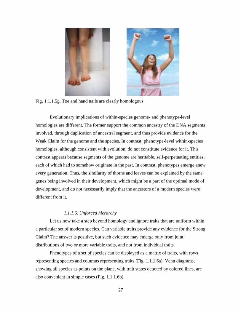
function but are similar to the corresponding genes (Fig. 1.1.1.5f). At higher levels, hand

and toe nails are made of the same keratins (Fig. 1.1.1.5g), and in many plants thorns are

unnecessarily similar to leaves or twigs.

cagctcaccatggatgatgatatcaccgcgctcgtcattgacaacggctc

|||||||||||||||||||||||| ||||||||||| | |||||||||||

cagctcaccatggatgatgatatcgccgcgctcgtcgtcgacaacggctc

cggcatgtgcaaggccagcttcacgggcgacaatgccgcccgggcagtct

|||||||||||||||| ||||| |||||||| ||||| ||||||| ||||

cggcatgtgcaaggccggcttcgcgggcgacgatgccccccgggccgtct

tcccctccatcgttgggcaccccaggcaccag------------------

||||||||||||| |||| |||||||||||||

26

tcccctccatcgtggggcgccccaggcaccaggtaggggagctggctggg

--------------------------------------------------

tggggcagccccgggagcgggcgggaggcaagggcgctttctctgcacag

--------------------------------------------------

gagcctcccggtttccggggtgggggctgcgcccgtgctcagggcttctt

----------------ggcgtgatggtgggcatgggtcagaaggattcct

||||||||||||||||||||||||||||||||||

gtcctttccttcccagggcgtgatggtgggcatgggtcagaaggattcct

atgtgggcgacgaggcccagagcaagagaggcat

||||||||||||||||||||||||||||||||||

atgtgggcgacgaggcccagagcaagagaggcat

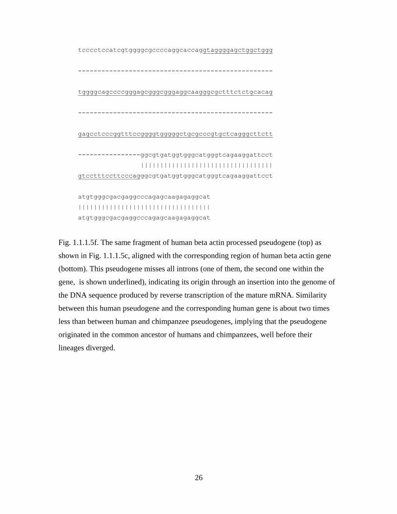
Fig. 1.1.1.5f. The same fragment of human beta actin processed pseudogene (top) as

shown in Fig. 1.1.1.5c, aligned with the corresponding region of human beta actin gene

(bottom). This pseudogene misses all introns (one of them, the second one within the

gene, is shown underlined), indicating its origin through an insertion into the genome of

the DNA sequence produced by reverse transcription of the mature mRNA. Similarity

between this human pseudogene and the corresponding human gene is about two times

less than between human and chimpanzee pseudogenes, implying that the pseudogene

originated in the common ancestor of humans and chimpanzees, well before their

lineages diverged.

27

Fig. 1.1.1.5g. Toe and hand nails are clearly homologous.

Evolutionary implications of within-species genome- and phenotype-level

homologies are different. The former support the common ancestry of the DNA segments

involved, through duplication of ancestral segment, and thus provide evidence for the

Weak Claim for the genome and the species. In contrast, phenotype-level within-species

homologies, although consistent with evolution, do not constitute evidence for it. This

contrast appears because segments of the genome are heritable, self-perpetuating entities,

each of which had to somehow originate in the past. In contrast, phenotypes emerge anew

every generation. Thus, the similarity of thorns and leaves can be explained by the same

genes being involved in their development, which might be a part of the optimal mode of

development, and do not necessarily imply that the ancestors of a modern species were

different from it.

1.1.1.6. Unforced hierarchy

Let us now take a step beyond homology and ignore traits that are uniform within

a particular set of modern species. Can variable traits provide any evidence for the Strong

Claim? The answer is positive, but such evidence may emerge only from joint

distributions of two or more variable traits, and not from individual traits.

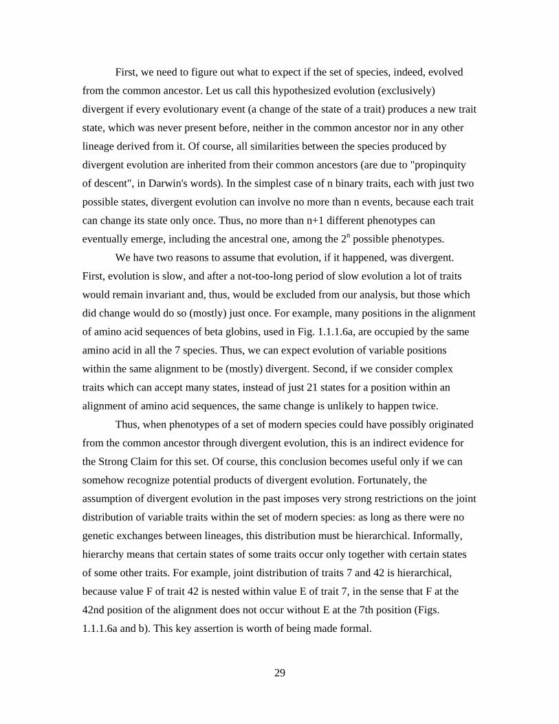
Phenotypes of a set of species can be displayed as a matrix of traits, with rows

representing species and columns representing traits (Fig. 1.1.1.6a). Venn diagrams,

showing all species as points on the plane, with trait states denoted by colored lines, are

also convenient in simple cases (Fig. 1.1.1.6b).

28

Traits:

Species: 7 9 12 33 34 42 57 79 116

Homo sapiens E K V L V F G L A

Monodelphis domestica E K I L V F G L G

Gallus gallus E K I L I F G L A

Rana catesbeiana E K I F I Y G L G

Hynobius retardatus E K I L I Y A L A

Salmo salar A K I L I Y G M A

Danio rerio A R I L I Y G M A

Fig. 1.1.1.6a. A matrix of traits presenting phenotypes of 7 species each consisting of 9

traits. Each trait characterizes a corresponding position in the alignment of beta globins

from these species, and the trait state is the amino acid that occupies this position. Only

binary traits, with just two states within the set of species, were chosen, and for each trait

one state is shown in red and the other in black. The species are human, gray short-tailed

opossum, chicken, North American bullfrog, Hokkaido salamander, Atlantic salmon, and

zebrafish.

Fig. 1.1.1.6b. Venn diagram representing data from Fig. 1.1.1.6a. For each trait, species

with the trait state shown in red in Fig. 1.1.1.6a are enclosed into a line of the

corresponding color.

29

First, we need to figure out what to expect if the set of species, indeed, evolved

from the common ancestor. Let us call this hypothesized evolution (exclusively)

divergent if every evolutionary event (a change of the state of a trait) produces a new trait

state, which was never present before, neither in the common ancestor nor in any other

lineage derived from it. Of course, all similarities between the species produced by

divergent evolution are inherited from their common ancestors (are due to "propinquity

of descent", in Darwin's words). In the simplest case of n binary traits, each with just two

possible states, divergent evolution can involve no more than n events, because each trait

can change its state only once. Thus, no more than n+1 different phenotypes can

eventually emerge, including the ancestral one, among the 2n possible phenotypes.

We have two reasons to assume that evolution, if it happened, was divergent.

First, evolution is slow, and after a not-too-long period of slow evolution a lot of traits

would remain invariant and, thus, would be excluded from our analysis, but those which

did change would do so (mostly) just once. For example, many positions in the alignment

of amino acid sequences of beta globins, used in Fig. 1.1.1.6a, are occupied by the same

amino acid in all the 7 species. Thus, we can expect evolution of variable positions

within the same alignment to be (mostly) divergent. Second, if we consider complex

traits which can accept many states, instead of just 21 states for a position within an

alignment of amino acid sequences, the same change is unlikely to happen twice.

Thus, when phenotypes of a set of modern species could have possibly originated

from the common ancestor through divergent evolution, this is an indirect evidence for

the Strong Claim for this set. Of course, this conclusion becomes useful only if we can

somehow recognize potential products of divergent evolution. Fortunately, the

assumption of divergent evolution in the past imposes very strong restrictions on the joint

distribution of variable traits within the set of modern species: as long as there were no

genetic exchanges between lineages, this distribution must be hierarchical. Informally,

hierarchy means that certain states of some traits occur only together with certain states

of some other traits. For example, joint distribution of traits 7 and 42 is hierarchical,

because value F of trait 42 is nested within value E of trait 7, in the sense that F at the

42nd position of the alignment does not occur without E at the 7th position (Figs.

1.1.1.6a and b). This key assertion is worth of being made formal.

30

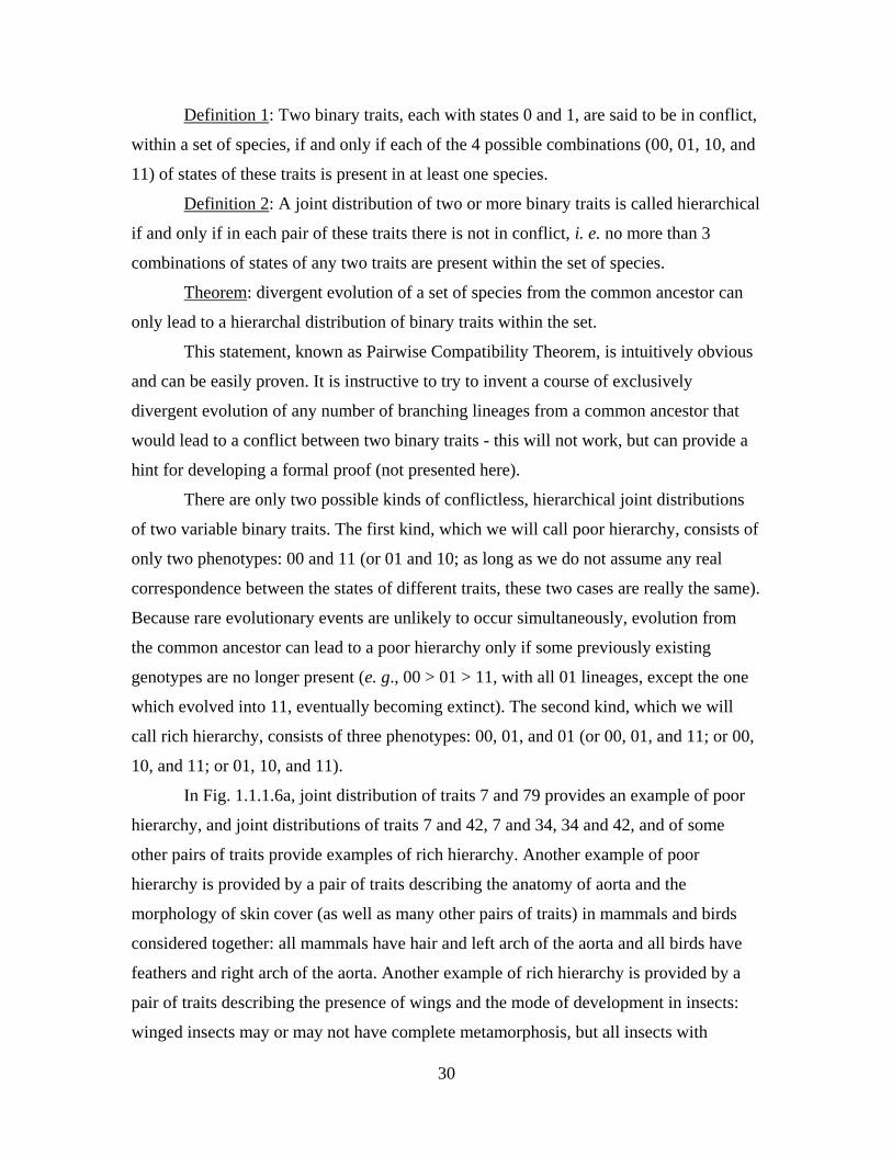
Definition 1: Two binary traits, each with states 0 and 1, are said to be in conflict,

within a set of species, if and only if each of the 4 possible combinations (00, 01, 10, and

11) of states of these traits is present in at least one species.

Definition 2: A joint distribution of two or more binary traits is called hierarchical

if and only if in each pair of these traits there is not in conflict, i. e. no more than 3

combinations of states of any two traits are present within the set of species.

Theorem: divergent evolution of a set of species from the common ancestor can

only lead to a hierarchal distribution of binary traits within the set.

This statement, known as Pairwise Compatibility Theorem, is intuitively obvious

and can be easily proven. It is instructive to try to invent a course of exclusively

divergent evolution of any number of branching lineages from a common ancestor that

would lead to a conflict between two binary traits - this will not work, but can provide a

hint for developing a formal proof (not presented here).

There are only two possible kinds of conflictless, hierarchical joint distributions

of two variable binary traits. The first kind, which we will call poor hierarchy, consists of

only two phenotypes: 00 and 11 (or 01 and 10; as long as we do not assume any real

correspondence between the states of different traits, these two cases are really the same).

Because rare evolutionary events are unlikely to occur simultaneously, evolution from

the common ancestor can lead to a poor hierarchy only if some previously existing

genotypes are no longer present (e. g., 00 > 01 > 11, with all 01 lineages, except the one

which evolved into 11, eventually becoming extinct). The second kind, which we will

call rich hierarchy, consists of three phenotypes: 00, 01, and 01 (or 00, 01, and 11; or 00,

10, and 11; or 01, 10, and 11).

In Fig. 1.1.1.6a, joint distribution of traits 7 and 79 provides an example of poor

hierarchy, and joint distributions of traits 7 and 42, 7 and 34, 34 and 42, and of some

other pairs of traits provide examples of rich hierarchy. Another example of poor

hierarchy is provided by a pair of traits describing the anatomy of aorta and the

morphology of skin cover (as well as many other pairs of traits) in mammals and birds

considered together: all mammals have hair and left arch of the aorta and all birds have

feathers and right arch of the aorta. Another example of rich hierarchy is provided by a

pair of traits describing the presence of wings and the mode of development in insects:

winged insects may or may not have complete metamorphosis, but all insects with

31

complete metamorphosis have wings. One can say that complete metamorphosis is nested

within possession of wings.

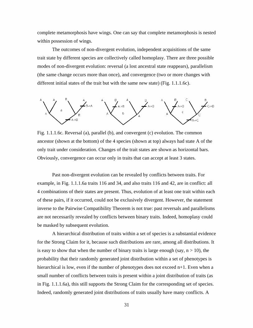
The outcomes of non-divergent evolution, independent acquisitions of the same

trait state by different species are collectively called homoplasy. There are three possible

modes of non-divergent evolution: reversal (a lost ancestral state reappears), parallelism

(the same change occurs more than once), and convergence (two or more changes with

different initial states of the trait but with the same new state) (Fig. 1.1.1.6c).

Fig. 1.1.1.6c. Reversal (a), parallel (b), and convergent (c) evolution. The common

ancestor (shown at the bottom) of the 4 species (shown at top) always had state A of the

only trait under consideration. Changes of the trait states are shown as horizontal bars.

Obviously, convergence can occur only in traits that can accept at least 3 states.

Past non-divergent evolution can be revealed by conflicts between traits. For

example, in Fig. 1.1.1.6a traits 116 and 34, and also traits 116 and 42, are in conflict: all

4 combinations of their states are present. Thus, evolution of at least one trait within each

of these pairs, if it occurred, could not be exclusively divergent. However, the statement

inverse to the Pairwise Compatibility Theorem is not true: past reversals and parallelisms

are not necessarily revealed by conflicts between binary traits. Indeed, homoplasy could

be masked by subsequent evolution.

A hierarchical distribution of traits within a set of species is a substantial evidence

for the Strong Claim for it, because such distributions are rare, among all distributions. It

is easy to show that when the number of binary traits is large enough (say, n > 10), the

probability that their randomly generated joint distribution within a set of phenotypes is

hierarchical is low, even if the number of phenotypes does not exceed n+1. Even when a

small number of conflicts between traits is present within a joint distribution of traits (as

in Fig. 1.1.1.6a), this still supports the Strong Claim for the corresponding set of species.

Indeed, randomly generated joint distributions of traits usually have many conflicts. A

32

predominantly hierarchical joint distribution of traits with a small number of conflicts can

be produced by mostly divergent evolution, with occasional homoplasy, which may be a

plausible situation. Defining traits properly is crucial for any comparative analysis of

phenotypes, including analysis of conflicts. Still, no definition of traits could impose

hierarchy on an intrinsically non-hierarchical set of phenotypes.

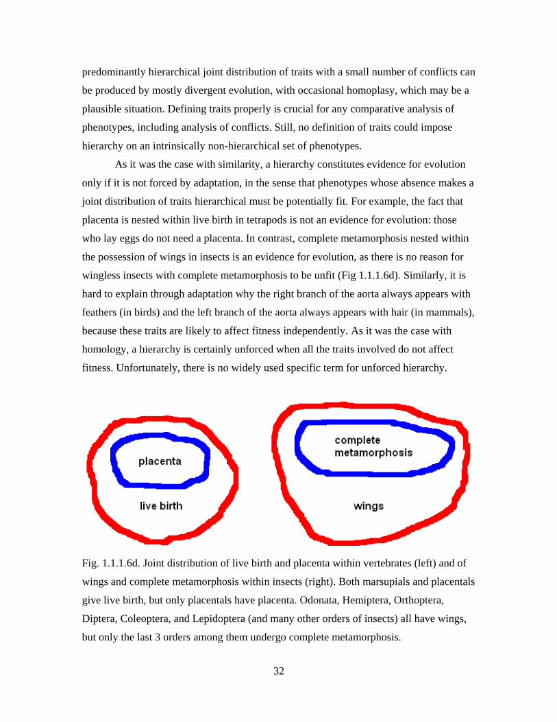
As it was the case with similarity, a hierarchy constitutes evidence for evolution

only if it is not forced by adaptation, in the sense that phenotypes whose absence makes a

joint distribution of traits hierarchical must be potentially fit. For example, the fact that

placenta is nested within live birth in tetrapods is not an evidence for evolution: those

who lay eggs do not need a placenta. In contrast, complete metamorphosis nested within

the possession of wings in insects is an evidence for evolution, as there is no reason for

wingless insects with complete metamorphosis to be unfit (Fig 1.1.1.6d). Similarly, it is

hard to explain through adaptation why the right branch of the aorta always appears with

feathers (in birds) and the left branch of the aorta always appears with hair (in mammals),

because these traits are likely to affect fitness independently. As it was the case with

homology, a hierarchy is certainly unforced when all the traits involved do not affect

fitness. Unfortunately, there is no widely used specific term for unforced hierarchy.

Fig. 1.1.1.6d. Joint distribution of live birth and placenta within vertebrates (left) and of

wings and complete metamorphosis within insects (right). Both marsupials and placentals

give live birth, but only placentals have placenta. Odonata, Hemiptera, Orthoptera,

Diptera, Coleoptera, and Lepidoptera (and many other orders of insects) all have wings,

but only the last 3 orders among them undergo complete metamorphosis.

33

Related, but more sophisticated analyses are possible for multistate traits,

although in this case it is harder to determine whether a particular matrix of traits can be

produced by exclusively divergent evolution. Still, joint distributions of multistate traits

which can be produced without homoplasy represent evidence for the Strong Claim for

the species involved. Hierarchical distributions of complex and slowly evolving traits

pervade all life and constitute a very important kind of indirect evidence for past

evolution.

1.1.1.7. Unforced similarity of geographical ranges

Data on geographical ranges of modern species, combined with data on their

phenotypes, produce yet another kind of indirect evidence for past evolution, based on

the assumption that, if evolution happened, the ranges of evolving species were generally

conservative. Occasionally, the range of a species may, in contrast to its phenotype,

change abruptly, due to a long-distance invasion or a local extinction. However, we may

assume that such changes were uncommon before human activity led to numerous

invasions and extinctions. So, what do we expect to see after slow evolution,

accompanied by limited dispersal?

Limited dispersal naturally leads to an expectation that the range of a species may

be suboptimal, in the sense that the species is absent from areas where it could thrive.

Indeed, recent human-mediated dispersal led to countless successful invasions, some of

them with disastrous consequences, and thus demonstrated that suboptimality of species

ranges is very common (Fig. 1.1.1.7a). In fact, an invasion demonstrates suboptimality of

the original range of the invader more directly than suboptimality of any phenotype could

be currently demonstrated. Moreover, there is a strong correlation between the ability of

a species to disperse and the degree of suboptimality of its range. In particular, before

being affected by humans, oceanic island were population mostly by species who are

more capable of dispersal, e. g., by birds much more than by mammals. For example,

there are only two native species of mammals in New Zealand, and both of them are bats.

Suboptimality of the range of a species is definitely an evidence for its localized origin.

However, in contrast to suboptimality of the phenotype, suboptimality of the range is not

34

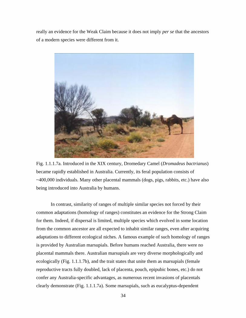
really an evidence for the Weak Claim because it does not imply per se that the ancestors

of a modern species were different from it.

Fig. 1.1.1.7a. Introduced in the XIX century, Dromedary Camel (Dromadeus bactrianus)

became rapidly established in Australia. Currently, its feral population consists of

~400,000 individuals. Many other placental mammals (dogs, pigs, rabbits, etc.) have also

being introduced into Australia by humans.

In contrast, similarity of ranges of multiple similar species not forced by their

common adaptations (homology of ranges) constitutes an evidence for the Strong Claim

for them. Indeed, if dispersal is limited, multiple species which evolved in some location

from the common ancestor are all expected to inhabit similar ranges, even after acquiring

adaptations to different ecological niches. A famous example of such homology of ranges

is provided by Australian marsupials. Before humans reached Australia, there were no

placental mammals there. Australian marsupials are very diverse morphologically and

ecologically (Fig. 1.1.1.7b), and the trait states that unite them as marsupials (female

reproductive tracts fully doubled, lack of placenta, pouch, epipubic bones, etc.) do not

confer any Australia-specific advantages, as numerous recent invasions of placentals

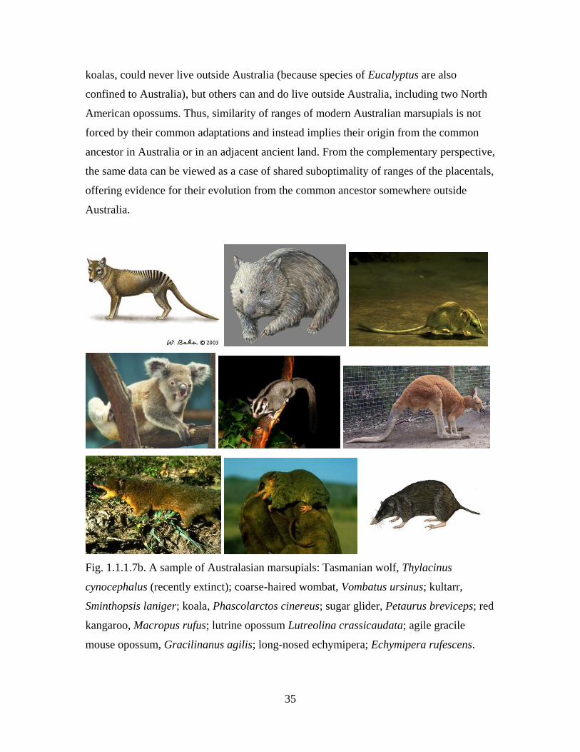
clearly demonstrate (Fig. 1.1.1.7a). Some marsupials, such as eucalyptus-dependent

35

koalas, could never live outside Australia (because species of Eucalyptus are also

confined to Australia), but others can and do live outside Australia, including two North

American opossums. Thus, similarity of ranges of modern Australian marsupials is not

forced by their common adaptations and instead implies their origin from the common

ancestor in Australia or in an adjacent ancient land. From the complementary perspective,

the same data can be viewed as a case of shared suboptimality of ranges of the placentals,

offering evidence for their evolution from the common ancestor somewhere outside

Australia.

Fig. 1.1.1.7b. A sample of Australasian marsupials: Tasmanian wolf, Thylacinus

cynocephalus (recently extinct); coarse-haired wombat, Vombatus ursinus; kultarr,

Sminthopsis laniger; koala, Phascolarctos cinereus; sugar glider, Petaurus breviceps; red

kangaroo, Macropus rufus; lutrine opossum Lutreolina crassicaudata; agile gracile

mouse opossum, Gracilinanus agilis; long-nosed echymipera; Echymipera rufescens.

36

There is a striking, although superficial, resemblance within many pairs of

placentals and Australian marsupials, such as wolf and "Tasmanian wolf", mole and

"marsupial mole", etc. Of course, such resemblances, being forced by similarity of

adaptations, do not provide any evidence for evolution. Instead, evidence for evolution is

provided by the common "marsupial" trait states and ranges of "Tasmanian wolf",

"marsupial mole", etc., as well as by common "placental" trait states and ranges of the

corresponding placentals.

More complex patterns in joint distributions of ranges of multiple species,

considered below, can also offer support for their evolution from the common ancestor

accompanied by mostly slow dispersal. Such patterns are encountered everywhere and

provide an important and fascinating kind of indirect evidence for past evolution.

1.1.1.8. Evolutionary scenarios and theories

Evidence for evolution presented so far are very basic in nature - they simply

emerge from comparing properties of modern species to what can be expected if they

were produced by gradual, slow, and greedy evolution, perhaps accompanied by limited

dispersal. On top of this, we can sometimes formulate more specific hypotheses on how

evolution, if any, may occur and what outcomes it may produce.

It is convenient to think of two kinds of such hypotheses. First, they can be based

on simple, plausible scenarios for past evolution. Second, the already available rudiments

of theory of evolution can lead to more sophisticated analyses. If what we observe agrees

with what is implied by an evolutionary scenario or theory, a scenario-based or a theory-

based indirect evidence for past evolution emerges. Currently, different evidence of these

kinds are mostly disconnected from each other, due to lack of a comprehensive theory of

evolution.

An example of a plausible, specific evolutionary scenario is provided by whole-

genome duplications (WGDs). Such duplications, converting a diploid into an

autotetraploid, have been observed directly, and there are modern species where diploids

and autotetraploids coexist. However, there are also species whose genomes mostly

consist of pairs of similar segments, usually located on different chromosomes. Segments

that constitute such a pair contain successive pairs of similar genes, arranged in the same

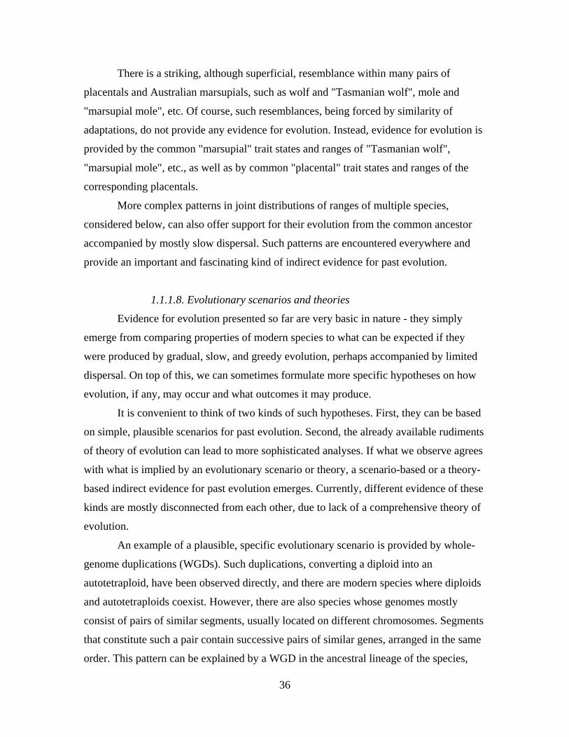
order. This pattern can be explained by a WGD in the ancestral lineage of the species,

37

followed by divergence between the two copies of the genome that involved large-scale

rearrangements that split them into segments, loss of some redundant duplicated genes,

and divergence within the remaining pairs of duplicated genes (Fig. 1.1.1.8a). A structure

of the genome of a modern species which implies that its lineage went through a WGD

followed by divergence between the two copies of the genome is an evidence for the

Weak Claim for this species. If genomes of multiple similar species all bear traces of an

ancestral WGD, this is an evidence for the Strong Claim for these species.

Figure 1.1.1.8a. A scenario of evolution following a whole-genome duplication. The box

at the top shows a hypothetical genome region containing ten genes numbered 1-10.

After WGD, the whole region is briefly present in two copies. However, many genes

subsequently return to single-copy state because one copy can be lost without the loss of

the corresponding function. In this example, only genes 1, 6 and 10 remain duplicated,

but the arrangement of these three pairs of homologous genes in the genome of a post-

WGD species (bottom) would be sufficient to detect a duplicated region using that

genome alone. Also, the gene order in each duplicated region in a post-WGD species

have a clear relationship to the gene order which existed in the pre-WGD genome (top),

and which may still be retained in species that diverged from the WGD lineage before the

WGD occurred (Phil. Trans. Roy. Soc. B 361, 403, 2006).

38

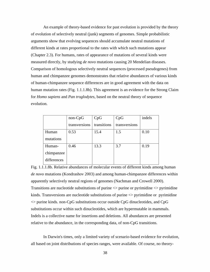
An example of theory-based evidence for past evolution is provided by the theory

of evolution of selectively neutral (junk) segments of genomes. Simple probabilistic

arguments show that evolving sequences should accumulate neutral mutations of

different kinds at rates proportional to the rates with which such mutations appear

(Chapter 2.3). For humans, rates of appearance of mutations of several kinds were

measured directly, by studying de novo mutations causing 20 Mendelian diseases.

Comparison of homologous selectively neutral sequences (processed pseudogenes) from

human and chimpanzee genomes demonstrates that relative abundances of various kinds

of human-chimpanzee sequence differences are in good agreement with the data on

human mutation rates (Fig. 1.1.1.8b). This agreement is an evidence for the Strong Claim

for Homo sapiens and Pan troglodytes, based on the neutral theory of sequence

evolution.

non-CpG

transversions

CpG

transitions

CpG

transversions

indels

Human

mutations

0.53 15.4 1.5 0.10

Human-

chimpanzee

differences

0.46 13.3 3.7 0.19

Fig. 1.1.1.8b. Relative abundances of molecular events of different kinds among human

de novo mutations (Kondrashov 2003) and among human-chimpanzee differences within

apparently selectively neutral regions of genomes (Nachman and Crowell 2000).

Transitions are nucleotide substitutions of purine <> purine or pyrimidine <> pyrimidine

kinds. Transversions are nucleotide substitutions of purine <> pyrimidine or pyrimidine

<> purine kinds. non-CpG substitutions occur outside CpG dinucleotides, and CpG

substitutions occur within such dinucleotides, which are hypermutable in mammals.

Indels is a collective name for insertions and deletions. All abundances are presented

relative to the abundance, in the corresponding data, of non-CpG transitions.

In Darwin's times, only a limited variety of scenario-based evidence for evolution,

all based on joint distributions of species ranges, were available. Of course, no theory-

39

based evidence were possible until well into the XX century. Currently, the variety of

scenario- and theory-based indirect evidence for past evolution is growing, as our

understanding of evolution improves, leading to new scenarios and theories.

Section 1.1.2. Examples of indirect evidence for past evolution

Diversity and complexity of modern life harbors countless evidence for its past

evolution. Many of these evidence were first recognized by Darwin, while others have

been discovered much more recently, in particular, in the course of the genomic

revolution. Here, a number of examples of indirect evidence of all kinds, concerned with

all levels of organization of life, is presented. These examples illustrate the reasoning

outlined in the previous Section and sometimes develop it further. Together, indirect

evidence for past evolution establish evolutionary origin of modern life as a fact.

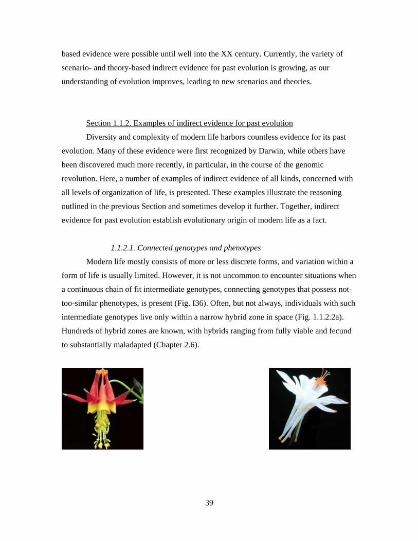
1.1.2.1. Connected genotypes and phenotypes

Modern life mostly consists of more or less discrete forms, and variation within a

form of life is usually limited. However, it is not uncommon to encounter situations when

a continuous chain of fit intermediate genotypes, connecting genotypes that possess not-

too-similar phenotypes, is present (Fig. I36). Often, but not always, individuals with such

intermediate genotypes live only within a narrow hybrid zone in space (Fig. 1.1.2.2a).

Hundreds of hybrid zones are known, with hybrids ranging from fully viable and fecund

to substantially maladapted (Chapter 2.6).

40

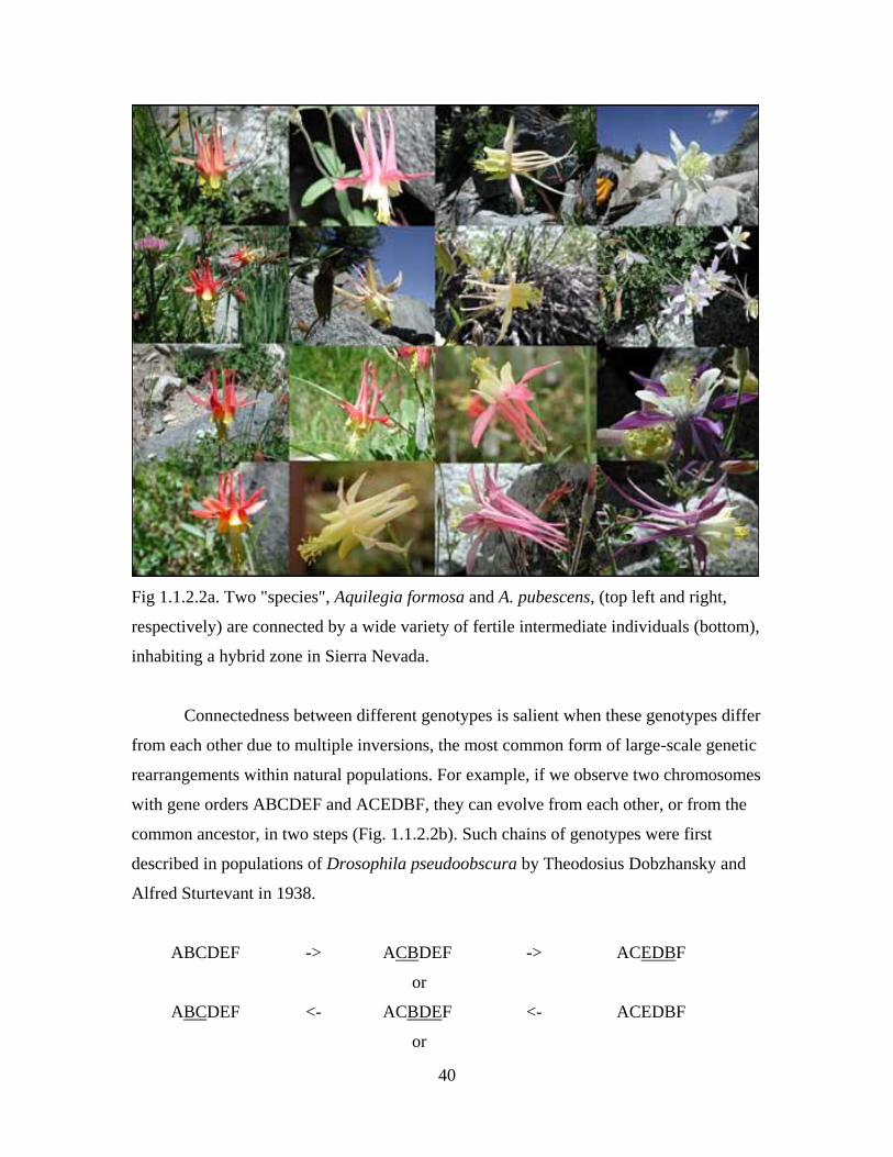
Fig 1.1.2.2a. Two "species", Aquilegia formosa and A. pubescens, (top left and right,

respectively) are connected by a wide variety of fertile intermediate individuals (bottom),

inhabiting a hybrid zone in Sierra Nevada.

Connectedness between different genotypes is salient when these genotypes differ

from each other due to multiple inversions, the most common form of large-scale genetic

rearrangements within natural populations. For example, if we observe two chromosomes

with gene orders ABCDEF and ACEDBF, they can evolve from each other, or from the

common ancestor, in two steps (Fig. 1.1.2.2b). Such chains of genotypes were first

described in populations of Drosophila pseudoobscura by Theodosius Dobzhansky and

Alfred Sturtevant in 1938.

ABCDEF -> ACBDEF -> ACEDBF

or

ABCDEF <- ACBDEF <- ACEDBF

or

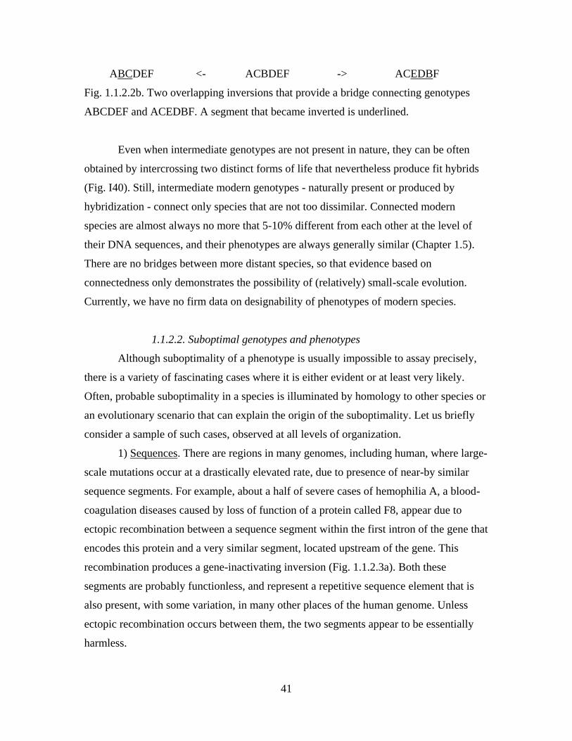
41

ABCDEF <- ACBDEF -> ACEDBF

Fig. 1.1.2.2b. Two overlapping inversions that provide a bridge connecting genotypes

ABCDEF and ACEDBF. A segment that became inverted is underlined.

Even when intermediate genotypes are not present in nature, they can be often

obtained by intercrossing two distinct forms of life that nevertheless produce fit hybrids

(Fig. I40). Still, intermediate modern genotypes - naturally present or produced by

hybridization - connect only species that are not too dissimilar. Connected modern

species are almost always no more that 5-10% different from each other at the level of

their DNA sequences, and their phenotypes are always generally similar (Chapter 1.5).

There are no bridges between more distant species, so that evidence based on

connectedness only demonstrates the possibility of (relatively) small-scale evolution.

Currently, we have no firm data on designability of phenotypes of modern species.

1.1.2.2. Suboptimal genotypes and phenotypes

Although suboptimality of a phenotype is usually impossible to assay precisely,

there is a variety of fascinating cases where it is either evident or at least very likely.

Often, probable suboptimality in a species is illuminated by homology to other species or

an evolutionary scenario that can explain the origin of the suboptimality. Let us briefly

consider a sample of such cases, observed at all levels of organization.

1) Sequences. There are regions in many genomes, including human, where large-

scale mutations occur at a drastically elevated rate, due to presence of near-by similar

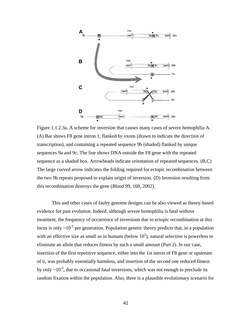
sequence segments. For example, about a half of severe cases of hemophilia A, a blood-

coagulation diseases caused by loss of function of a protein called F8, appear due to

ectopic recombination between a sequence segment within the first intron of the gene that

encodes this protein and a very similar segment, located upstream of the gene. This

recombination produces a gene-inactivating inversion (Fig. 1.1.2.3a). Both these

segments are probably functionless, and represent a repetitive sequence element that is

also present, with some variation, in many other places of the human genome. Unless

ectopic recombination occurs between them, the two segments appear to be essentially

harmless.

42

Figure 1.1.2.3a. A scheme for inversion that causes many cases of severe hemophilia A.

(A) Bar shows F8 gene intron 1, flanked by exons (drawn to indicate the direction of

transcription), and containing a repeated sequence 9b (shaded) flanked by unique

sequences 9a and 9c. The line shows DNA outside the F8 gene with the repeated

sequence as a shaded box. Arrowheads indicate orientation of repeated sequences. (B,C)

The large curved arrow indicates the folding required for ectopic recombination between

the two 9b repeats proposed to explain origin of inversion. (D) Inversion resulting from

this recombination destroys the gene (Blood 99, 168, 2002).

This and other cases of faulty genome designs can be also viewed as theory-based

evidence for past evolution. Indeed, although severe hemophilia is fatal without

treatment, the frequency of occurrence of inversions due to ectopic recombination at this

locus is only ~10-5

per generation. Population genetic theory predicts that, in a population

with an effective size as small as in humans (below 105), natural selection is powerless to

eliminate an allele that reduces fitness by such a small amount (Part 2). In our case,

insertion of the first repetitive sequence, either into the 1st intron of F8 gene or upstream

of it, was probably essentially harmless, and insertion of the second one reduced fitness

by only ~10-5

, due to occasional fatal inversions, which was not enough to preclude its

random fixation within the population. Also, there is a plausible evolutionary scenario for

43

the origin of these repeats, through duplication of other sequence segments belonging to

the same family of repetitive sequences (Section 1.1.2.6).

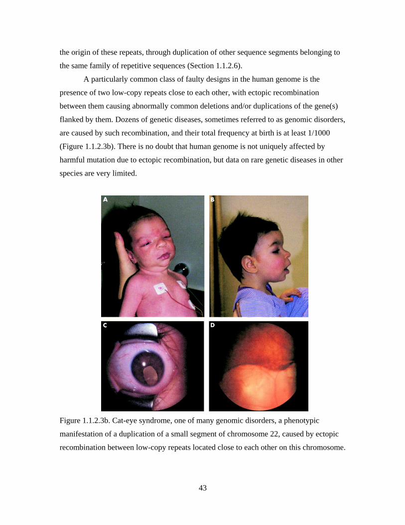
A particularly common class of faulty designs in the human genome is the

presence of two low-copy repeats close to each other, with ectopic recombination

between them causing abnormally common deletions and/or duplications of the gene(s)

flanked by them. Dozens of genetic diseases, sometimes referred to as genomic disorders,

are caused by such recombination, and their total frequency at birth is at least 1/1000

(Figure 1.1.2.3b). There is no doubt that human genome is not uniquely affected by

harmful mutation due to ectopic recombination, but data on rare genetic diseases in other

species are very limited.

Figure 1.1.2.3b. Cat-eye syndrome, one of many genomic disorders, a phenotypic

manifestation of a duplication of a small segment of chromosome 22, caused by ectopic

recombination between low-copy repeats located close to each other on this chromosome.

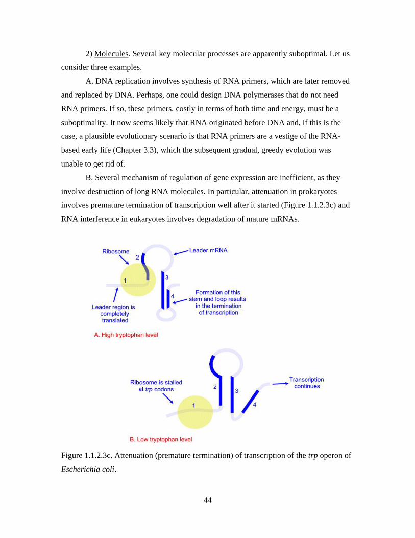
44

2) Molecules. Several key molecular processes are apparently suboptimal. Let us

consider three examples.

A. DNA replication involves synthesis of RNA primers, which are later removed

and replaced by DNA. Perhaps, one could design DNA polymerases that do not need

RNA primers. If so, these primers, costly in terms of both time and energy, must be a

suboptimality. It now seems likely that RNA originated before DNA and, if this is the

case, a plausible evolutionary scenario is that RNA primers are a vestige of the RNA-

based early life (Chapter 3.3), which the subsequent gradual, greedy evolution was

unable to get rid of.

B. Several mechanism of regulation of gene expression are inefficient, as they

involve destruction of long RNA molecules. In particular, attenuation in prokaryotes

involves premature termination of transcription well after it started (Figure 1.1.2.3c) and

RNA interference in eukaryotes involves degradation of mature mRNAs.

Figure 1.1.2.3c. Attenuation (premature termination) of transcription of the trp operon of

Escherichia coli.

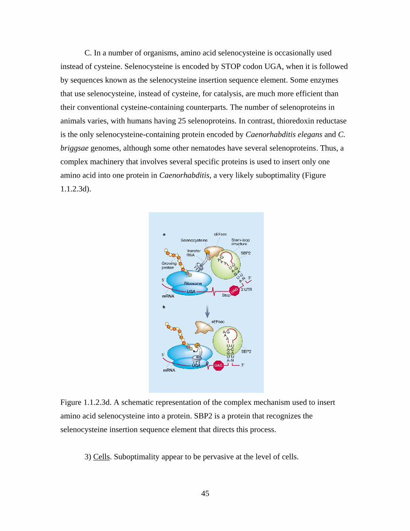
45

C. In a number of organisms, amino acid selenocysteine is occasionally used

instead of cysteine. Selenocysteine is encoded by STOP codon UGA, when it is followed

by sequences known as the selenocysteine insertion sequence element. Some enzymes

that use selenocysteine, instead of cysteine, for catalysis, are much more efficient than

their conventional cysteine-containing counterparts. The number of selenoproteins in

animals varies, with humans having 25 selenoproteins. In contrast, thioredoxin reductase

is the only selenocysteine-containing protein encoded by Caenorhabditis elegans and C.

briggsae genomes, although some other nematodes have several selenoproteins. Thus, a

complex machinery that involves several specific proteins is used to insert only one

amino acid into one protein in Caenorhabditis, a very likely suboptimality (Figure

1.1.2.3d).

Figure 1.1.2.3d. A schematic representation of the complex mechanism used to insert

amino acid selenocysteine into a protein. SBP2 is a protein that recognizes the

selenocysteine insertion sequence element that directs this process.

3) Cells. Suboptimality appear to be pervasive at the level of cells.

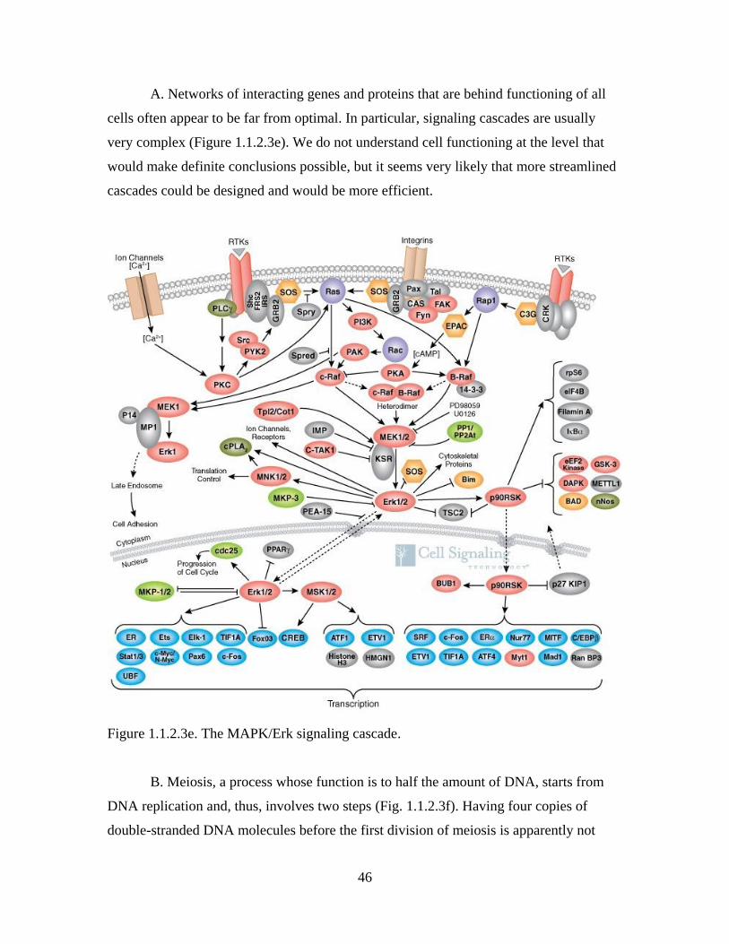
46

A. Networks of interacting genes and proteins that are behind functioning of all

cells often appear to be far from optimal. In particular, signaling cascades are usually

very complex (Figure 1.1.2.3e). We do not understand cell functioning at the level that

would make definite conclusions possible, but it seems very likely that more streamlined

cascades could be designed and would be more efficient.

Figure 1.1.2.3e. The MAPK/Erk signaling cascade.

B. Meiosis, a process whose function is to half the amount of DNA, starts from

DNA replication and, thus, involves two steps (Fig. 1.1.2.3f). Having four copies of

double-stranded DNA molecules before the first division of meiosis is apparently not

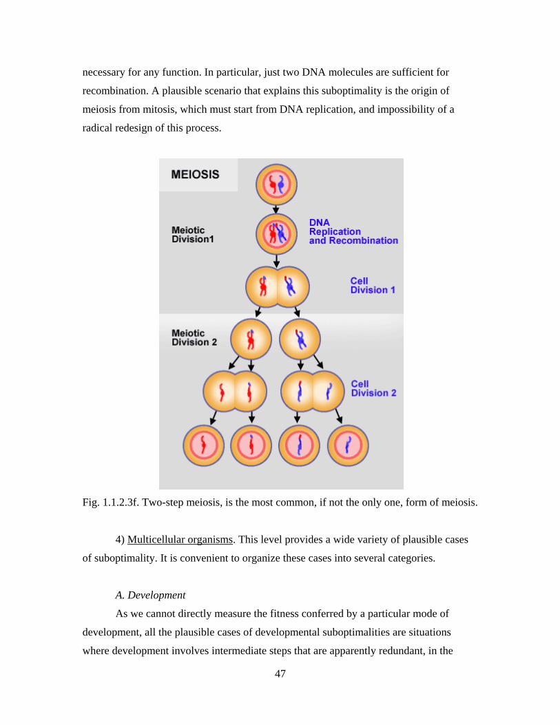
47

necessary for any function. In particular, just two DNA molecules are sufficient for

recombination. A plausible scenario that explains this suboptimality is the origin of

meiosis from mitosis, which must start from DNA replication, and impossibility of a

radical redesign of this process.

Fig. 1.1.2.3f. Two-step meiosis, is the most common, if not the only one, form of meiosis.

4) Multicellular organisms. This level provides a wide variety of plausible cases

of suboptimality. It is convenient to organize these cases into several categories.

A. Development

As we cannot directly measure the fitness conferred by a particular mode of

development, all the plausible cases of developmental suboptimalities are situations

where development involves intermediate steps that are apparently redundant, in the

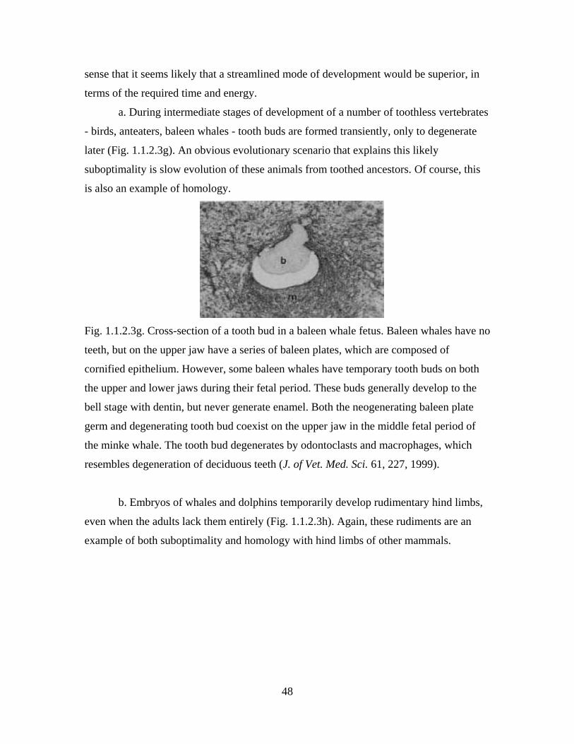
48

sense that it seems likely that a streamlined mode of development would be superior, in

terms of the required time and energy.

a. During intermediate stages of development of a number of toothless vertebrates

- birds, anteaters, baleen whales - tooth buds are formed transiently, only to degenerate

later (Fig. 1.1.2.3g). An obvious evolutionary scenario that explains this likely

suboptimality is slow evolution of these animals from toothed ancestors. Of course, this

is also an example of homology.

Fig. 1.1.2.3g. Cross-section of a tooth bud in a baleen whale fetus. Baleen whales have no

teeth, but on the upper jaw have a series of baleen plates, which are composed of

cornified epithelium. However, some baleen whales have temporary tooth buds on both

the upper and lower jaws during their fetal period. These buds generally develop to the

bell stage with dentin, but never generate enamel. Both the neogenerating baleen plate

germ and degenerating tooth bud coexist on the upper jaw in the middle fetal period of

the minke whale. The tooth bud degenerates by odontoclasts and macrophages, which

resembles degeneration of deciduous teeth (J. of Vet. Med. Sci. 61, 227, 1999).

b. Embryos of whales and dolphins temporarily develop rudimentary hind limbs,

even when the adults lack them entirely (Fig. 1.1.2.3h). Again, these rudiments are an

example of both suboptimality and homology with hind limbs of other mammals.

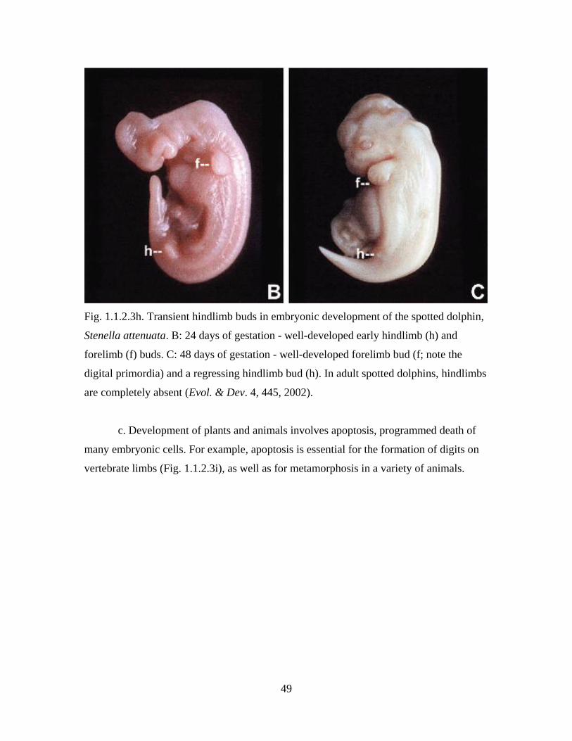
49

Fig. 1.1.2.3h. Transient hindlimb buds in embryonic development of the spotted dolphin,

Stenella attenuata. B: 24 days of gestation - well-developed early hindlimb (h) and

forelimb (f) buds. C: 48 days of gestation - well-developed forelimb bud (f; note the

digital primordia) and a regressing hindlimb bud (h). In adult spotted dolphins, hindlimbs

are completely absent (Evol. & Dev. 4, 445, 2002).

c. Development of plants and animals involves apoptosis, programmed death of

many embryonic cells. For example, apoptosis is essential for the formation of digits on

vertebrate limbs (Fig. 1.1.2.3i), as well as for metamorphosis in a variety of animals.

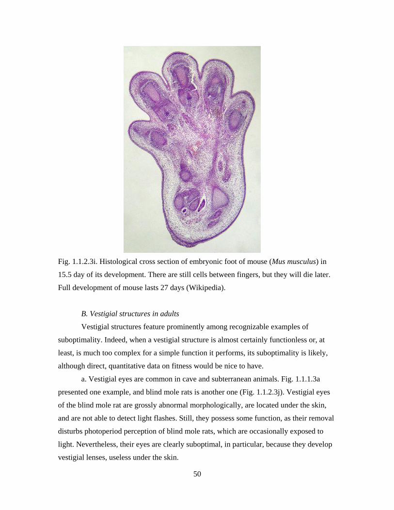
50

Fig. 1.1.2.3i. Histological cross section of embryonic foot of mouse (Mus musculus) in

15.5 day of its development. There are still cells between fingers, but they will die later.

Full development of mouse lasts 27 days (Wikipedia).

B. Vestigial structures in adults

Vestigial structures feature prominently among recognizable examples of

suboptimality. Indeed, when a vestigial structure is almost certainly functionless or, at

least, is much too complex for a simple function it performs, its suboptimality is likely,

although direct, quantitative data on fitness would be nice to have.

a. Vestigial eyes are common in cave and subterranean animals. Fig. 1.1.1.3a

presented one example, and blind mole rats is another one (Fig. 1.1.2.3j). Vestigial eyes

of the blind mole rat are grossly abnormal morphologically, are located under the skin,

and are not able to detect light flashes. Still, they possess some function, as their removal

disturbs photoperiod perception of blind mole rats, which are occasionally exposed to

light. Nevertheless, their eyes are clearly suboptimal, in particular, because they develop

vestigial lenses, useless under the skin.

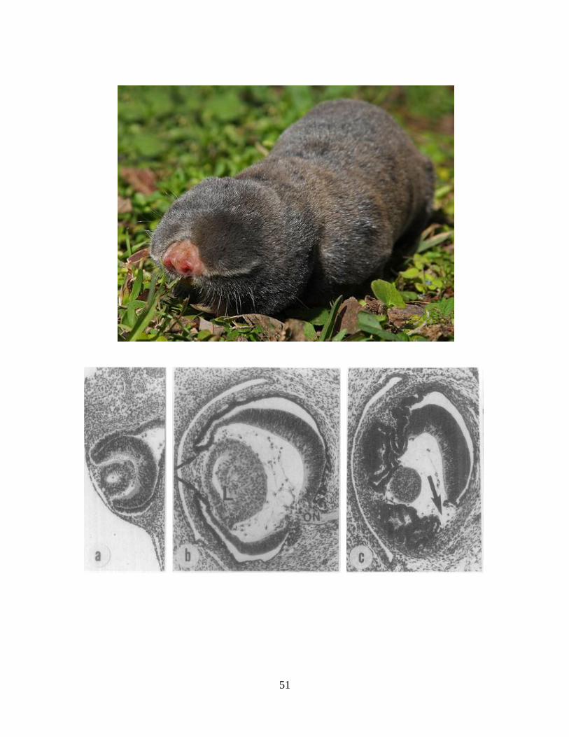
51

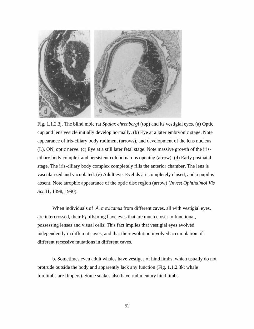
52

Fig. 1.1.2.3j. The blind mole rat Spalax ehrenbergi (top) and its vestigial eyes. (a) Optic

cup and lens vesicle initially develop normally. (b) Eye at a later embryonic stage. Note

appearance of iris-ciliary body rudiment (arrows), and development of the lens nucleus

(L). ON, optic nerve. (c) Eye at a still later fetal stage. Note massive growth of the iris-

ciliary body complex and persistent colobomatous opening (arrow). (d) Early postnatal

stage. The iris-ciliary body complex completely fills the anterior chamber. The lens is

vascularized and vacuolated. (e) Adult eye. Eyelids are completely closed, and a pupil is

absent. Note atrophic appearance of the optic disc region (arrow) (Invest Ophthalmol Vis

Sci 31, 1398, 1990).

When individuals of A. mexicanus from different caves, all with vestigial eyes,

are intercrossed, their F1 offspring have eyes that are much closer to functional,

possessing lenses and visual cells. This fact implies that vestigial eyes evolved

independently in different caves, and that their evolution involved accumulation of

different recessive mutations in different caves.

b. Sometimes even adult whales have vestiges of hind limbs, which usually do not

protrude outside the body and apparently lack any function (Fig. 1.1.2.3k; whale

forelimbs are flippers). Some snakes also have rudimentary hind limbs.

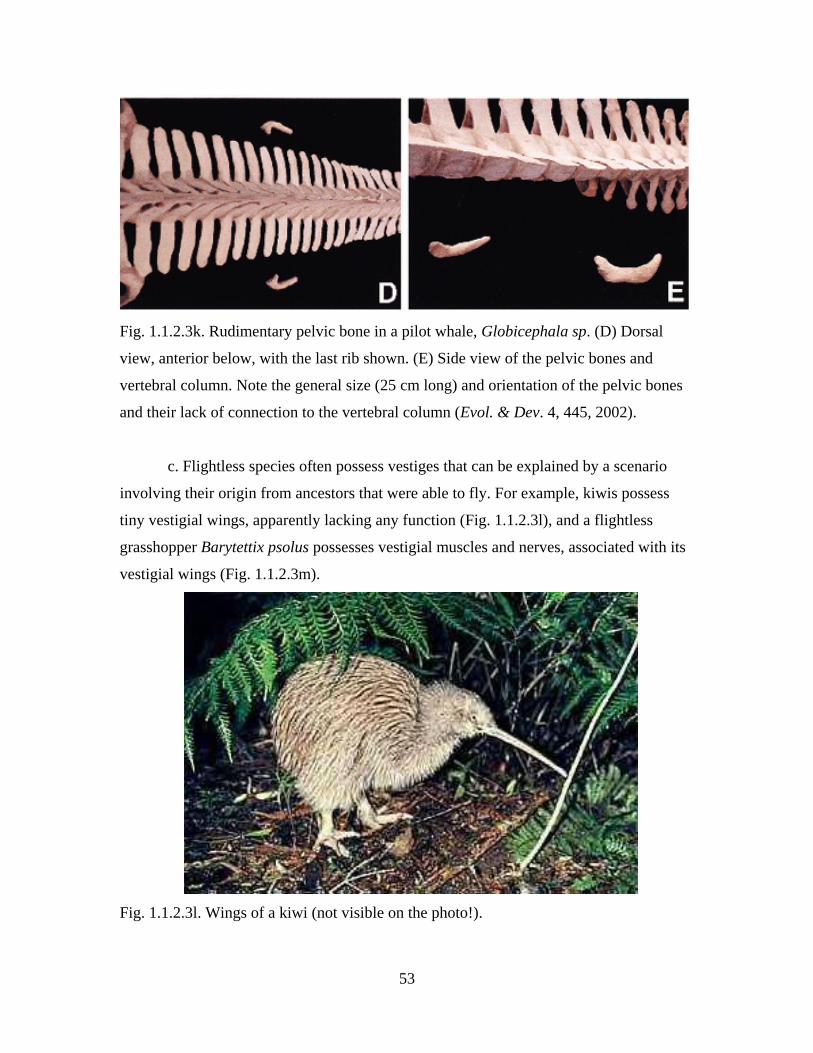
53

Fig. 1.1.2.3k. Rudimentary pelvic bone in a pilot whale, Globicephala sp. (D) Dorsal

view, anterior below, with the last rib shown. (E) Side view of the pelvic bones and

vertebral column. Note the general size (25 cm long) and orientation of the pelvic bones

and their lack of connection to the vertebral column (Evol. & Dev. 4, 445, 2002).

c. Flightless species often possess vestiges that can be explained by a scenario

involving their origin from ancestors that were able to fly. For example, kiwis possess

tiny vestigial wings, apparently lacking any function (Fig. 1.1.2.3l), and a flightless

grasshopper Barytettix psolus possesses vestigial muscles and nerves, associated with its

vestigial wings (Fig. 1.1.2.3m).

Fig. 1.1.2.3l. Wings of a kiwi (not visible on the photo!).

54

Fig. 1.1.2.3m. In a flightless grasshopper Barytettix psolus, adults lack flight muscles.

These muscles are present and innervated during nymphal life, but disappear in the adult.

Yet, their nerve persists and, in the adult, contains axonal presynaptic specializations

opposite inappropriate targets such as glia and basal lamina (bottom) (J. of Neurobiology

17, 627, 2004).

Functionless vestigial structures are likely to be easily improvable

suboptimalities. Some cave animals are completely eyeless, which is certainly optimal in

total darkness. If so, the presence of vestigial eyes may simply indicate that not enough

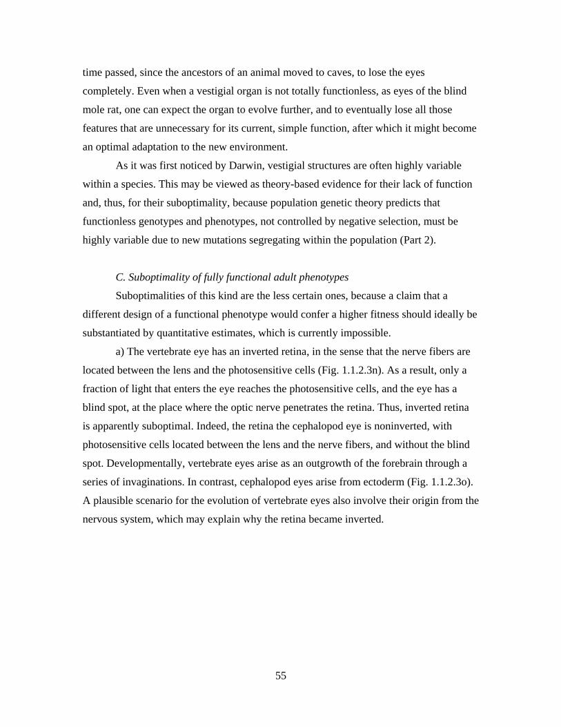
55

time passed, since the ancestors of an animal moved to caves, to lose the eyes

completely. Even when a vestigial organ is not totally functionless, as eyes of the blind

mole rat, one can expect the organ to evolve further, and to eventually lose all those

features that are unnecessary for its current, simple function, after which it might become

an optimal adaptation to the new environment.

As it was first noticed by Darwin, vestigial structures are often highly variable

within a species. This may be viewed as theory-based evidence for their lack of function

and, thus, for their suboptimality, because population genetic theory predicts that

functionless genotypes and phenotypes, not controlled by negative selection, must be

highly variable due to new mutations segregating within the population (Part 2).

C. Suboptimality of fully functional adult phenotypes

Suboptimalities of this kind are the less certain ones, because a claim that a

different design of a functional phenotype would confer a higher fitness should ideally be

substantiated by quantitative estimates, which is currently impossible.

a) The vertebrate eye has an inverted retina, in the sense that the nerve fibers are

located between the lens and the photosensitive cells (Fig. 1.1.2.3n). As a result, only a

fraction of light that enters the eye reaches the photosensitive cells, and the eye has a

blind spot, at the place where the optic nerve penetrates the retina. Thus, inverted retina

is apparently suboptimal. Indeed, the retina the cephalopod eye is noninverted, with

photosensitive cells located between the lens and the nerve fibers, and without the blind

spot. Developmentally, vertebrate eyes arise as an outgrowth of the forebrain through a

series of invaginations. In contrast, cephalopod eyes arise from ectoderm (Fig. 1.1.2.3o).

A plausible scenario for the evolution of vertebrate eyes also involve their origin from the

nervous system, which may explain why the retina became inverted.

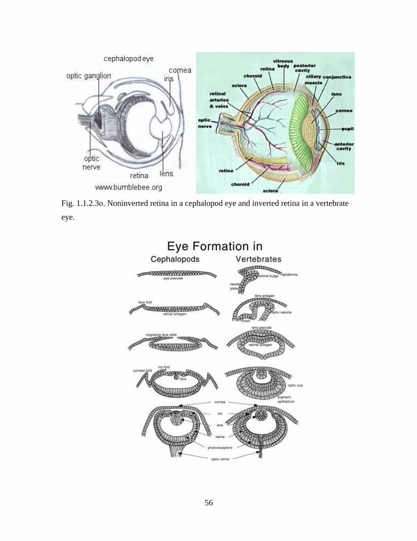
56

Fig. 1.1.2.3o. Noninverted retina in a cephalopod eye and inverted retina in a vertebrate

eye.

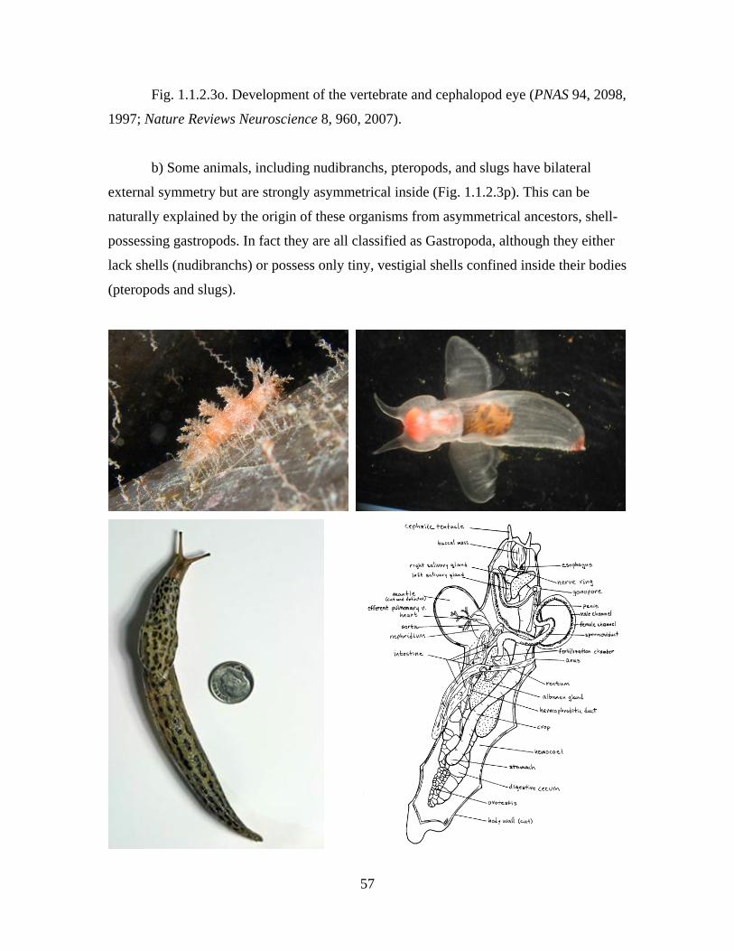
57

Fig. 1.1.2.3o. Development of the vertebrate and cephalopod eye (PNAS 94, 2098,

1997; Nature Reviews Neuroscience 8, 960, 2007).

b) Some animals, including nudibranchs, pteropods, and slugs have bilateral

external symmetry but are strongly asymmetrical inside (Fig. 1.1.2.3p). This can be

naturally explained by the origin of these organisms from asymmetrical ancestors, shell-

possessing gastropods. In fact they are all classified as Gastropoda, although they either

lack shells (nudibranchs) or possess only tiny, vestigial shells confined inside their bodies

(pteropods and slugs).

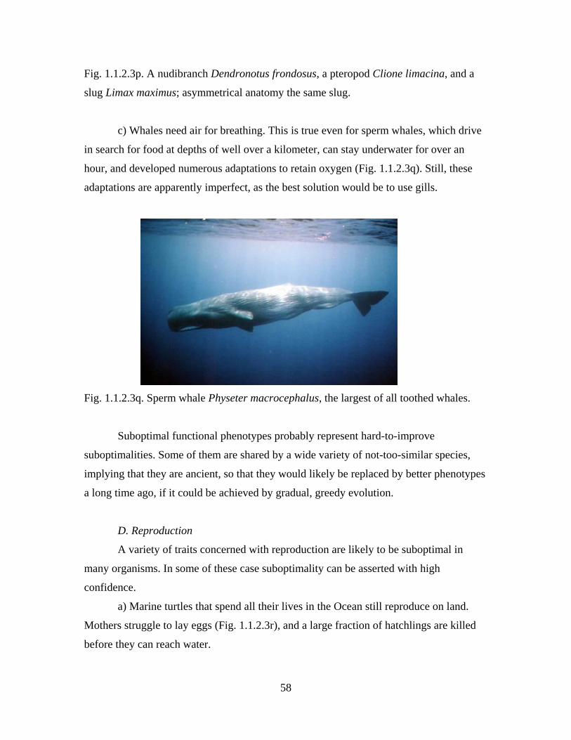
58

Fig. 1.1.2.3p. A nudibranch Dendronotus frondosus, a pteropod Clione limacina, and a

slug Limax maximus; asymmetrical anatomy the same slug.

c) Whales need air for breathing. This is true even for sperm whales, which drive

in search for food at depths of well over a kilometer, can stay underwater for over an

hour, and developed numerous adaptations to retain oxygen (Fig. 1.1.2.3q). Still, these

adaptations are apparently imperfect, as the best solution would be to use gills.

Fig. 1.1.2.3q. Sperm whale Physeter macrocephalus, the largest of all toothed whales.

Suboptimal functional phenotypes probably represent hard-to-improve

suboptimalities. Some of them are shared by a wide variety of not-too-similar species,

implying that they are ancient, so that they would likely be replaced by better phenotypes

a long time ago, if it could be achieved by gradual, greedy evolution.

D. Reproduction

A variety of traits concerned with reproduction are likely to be suboptimal in

many organisms. In some of these case suboptimality can be asserted with high

confidence.

a) Marine turtles that spend all their lives in the Ocean still reproduce on land.

Mothers struggle to lay eggs (Fig. 1.1.2.3r), and a large fraction of hatchlings are killed

before they can reach water.

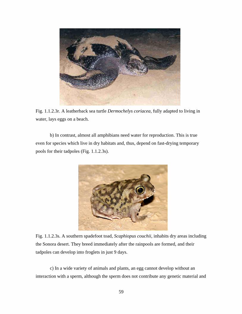
59

Fig. 1.1.2.3r. A leatherback sea turtle Dermochelys coriacea, fully adapted to living in

water, lays eggs on a beach.

b) In contrast, almost all amphibians need water for reproduction. This is true

even for species which live in dry habitats and, thus, depend on fast-drying temporary

pools for their tadpoles (Fig. 1.1.2.3s).

Fig. 1.1.2.3s. A southern spadefoot toad, Scaphiopus couchii, inhabits dry areas including

the Sonora desert. They breed immediately after the rainpools are formed, and their

tadpoles can develop into froglets in just 9 days.

c) In a wide variety of animals and plants, an egg cannot develop without an

interaction with a sperm, although the sperm does not contribute any genetic material and

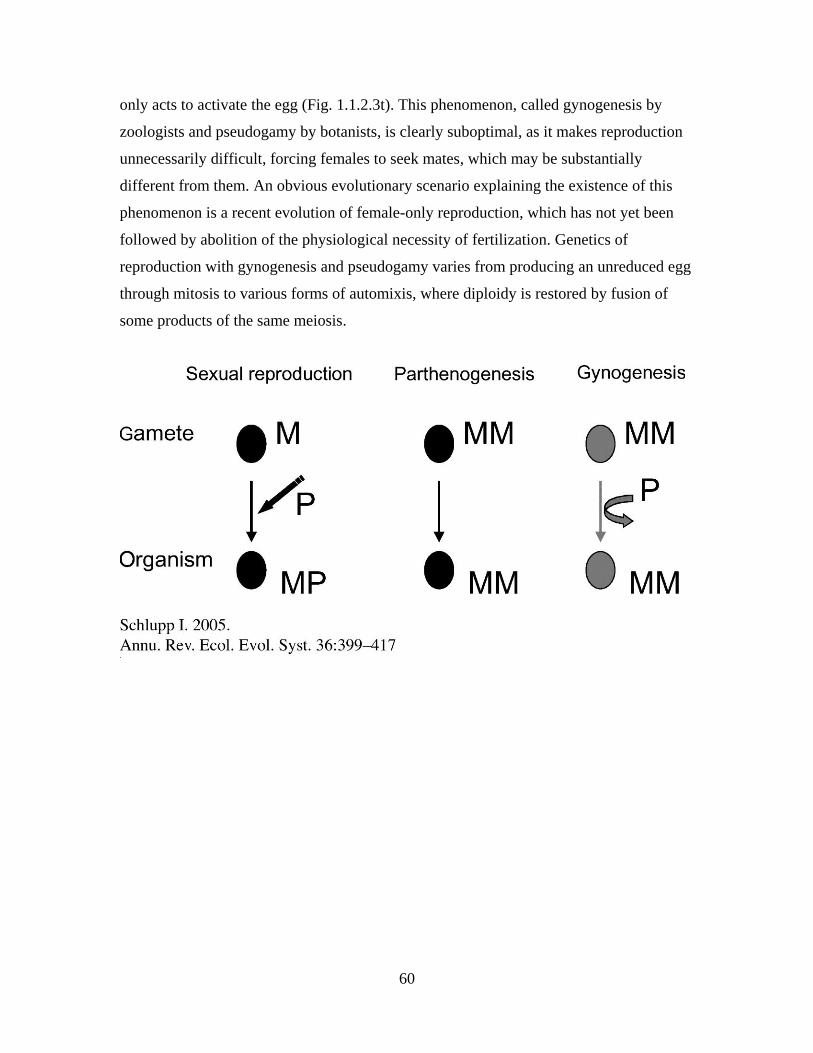
60

only acts to activate the egg (Fig. 1.1.2.3t). This phenomenon, called gynogenesis by

zoologists and pseudogamy by botanists, is clearly suboptimal, as it makes reproduction

unnecessarily difficult, forcing females to seek mates, which may be substantially

different from them. An obvious evolutionary scenario explaining the existence of this

phenomenon is a recent evolution of female-only reproduction, which has not yet been

followed by abolition of the physiological necessity of fertilization. Genetics of

reproduction with gynogenesis and pseudogamy varies from producing an unreduced egg

through mitosis to various forms of automixis, where diploidy is restored by fusion of

some products of the same meiosis.

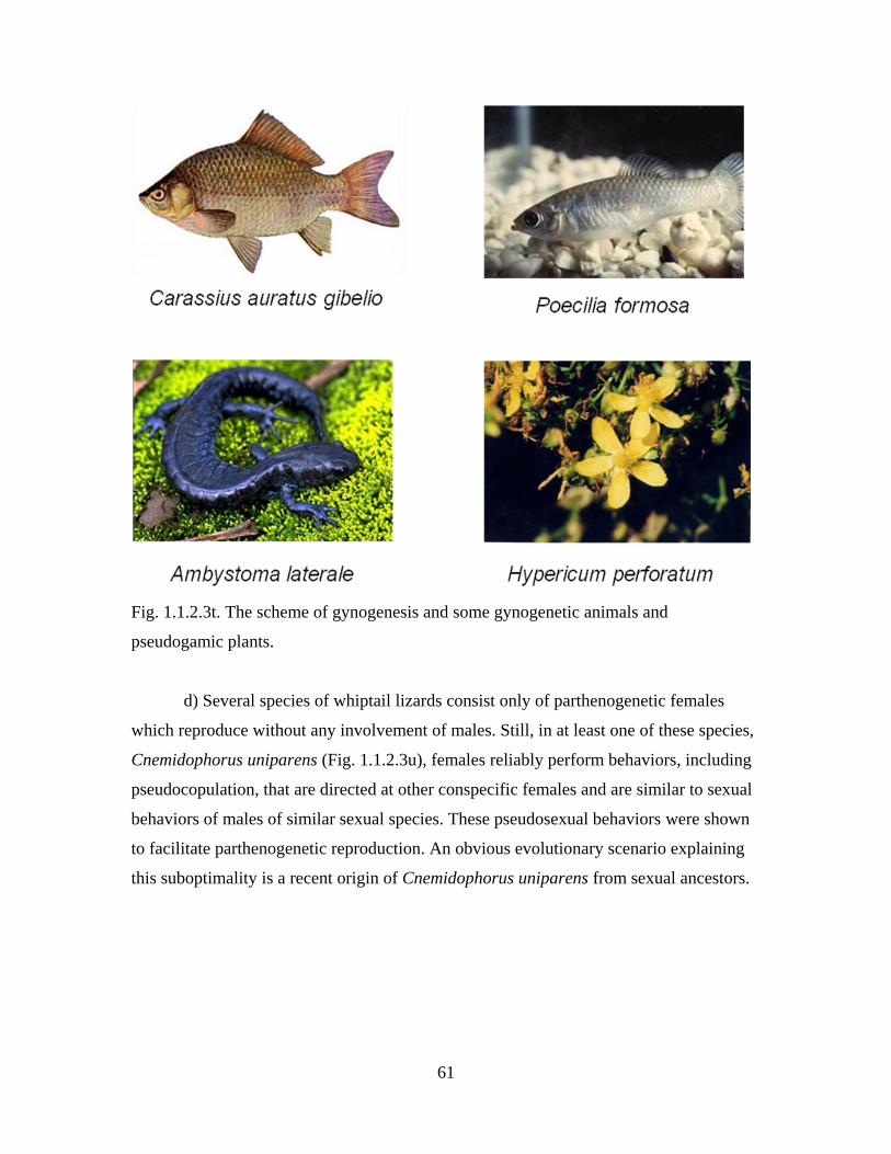
61

Fig. 1.1.2.3t. The scheme of gynogenesis and some gynogenetic animals and

pseudogamic plants.

d) Several species of whiptail lizards consist only of parthenogenetic females

which reproduce without any involvement of males. Still, in at least one of these species,

Cnemidophorus uniparens (Fig. 1.1.2.3u), females reliably perform behaviors, including

pseudocopulation, that are directed at other conspecific females and are similar to sexual

behaviors of males of similar sexual species. These pseudosexual behaviors were shown

to facilitate parthenogenetic reproduction. An obvious evolutionary scenario explaining

this suboptimality is a recent origin of Cnemidophorus uniparens from sexual ancestors.

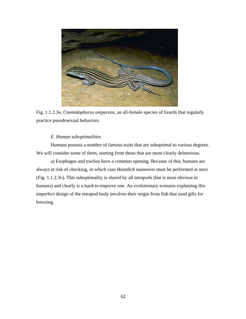
62

Fig. 1.1.2.3u. Cnemidophorus uniparens, an all-female species of lizards that regularly

practice pseudosexual behaviors.

E. Human suboptimalities

Humans possess a number of famous traits that are suboptimal to various degrees.

We will consider some of them, starting from those that are more clearly deleterious.

a) Esophagus and trachea have a common opening. Because of this, humans are

always at risk of chocking, in which case Heimlich maneuver must be performed at once

(Fig. 1.1.2.3v). This suboptimality is shared by all tetrapods (but is most obvious in

humans) and clearly is a hard-to-improve one. An evolutionary scenario explaining this

imperfect design of the tetrapod body involves their origin from fish that used gills for

breezing.

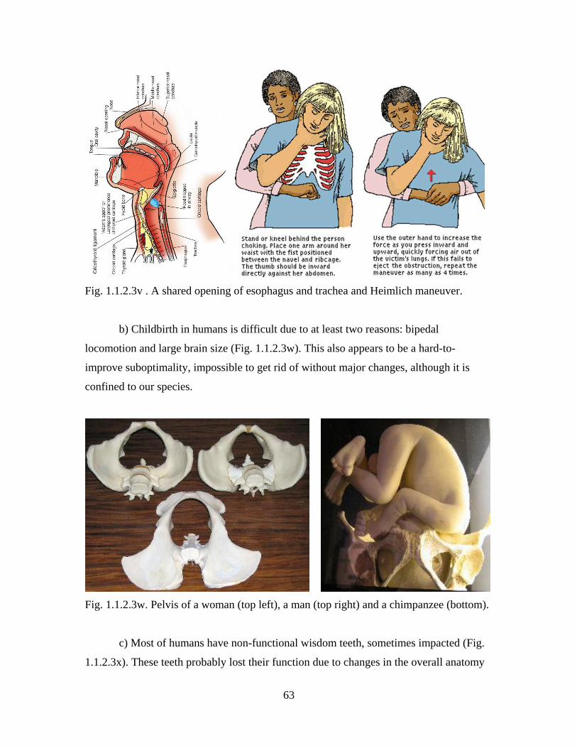
63

Fig. 1.1.2.3v . A shared opening of esophagus and trachea and Heimlich maneuver.

b) Childbirth in humans is difficult due to at least two reasons: bipedal

locomotion and large brain size (Fig. 1.1.2.3w). This also appears to be a hard-to-

improve suboptimality, impossible to get rid of without major changes, although it is

confined to our species.

Fig. 1.1.2.3w. Pelvis of a woman (top left), a man (top right) and a chimpanzee (bottom).

c) Most of humans have non-functional wisdom teeth, sometimes impacted (Fig.

1.1.2.3x). These teeth probably lost their function due to changes in the overall anatomy

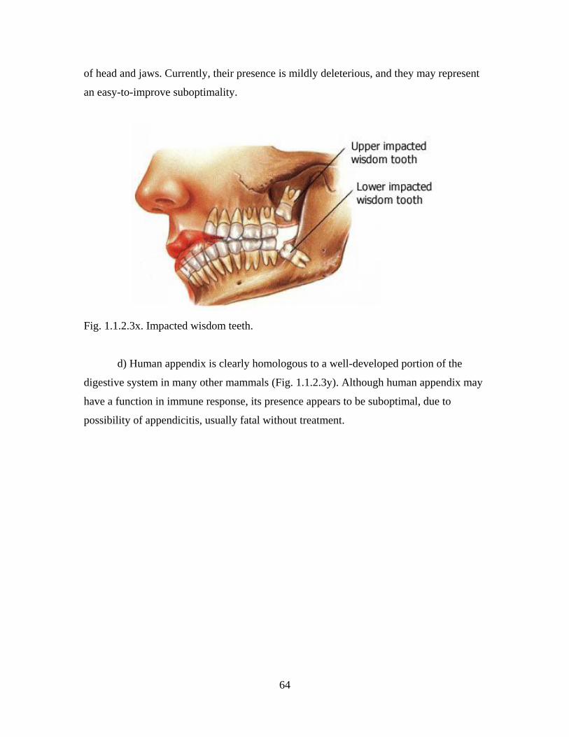
64

of head and jaws. Currently, their presence is mildly deleterious, and they may represent

an easy-to-improve suboptimality.

Fig. 1.1.2.3x. Impacted wisdom teeth.

d) Human appendix is clearly homologous to a well-developed portion of the

digestive system in many other mammals (Fig. 1.1.2.3y). Although human appendix may

have a function in immune response, its presence appears to be suboptimal, due to

possibility of appendicitis, usually fatal without treatment.

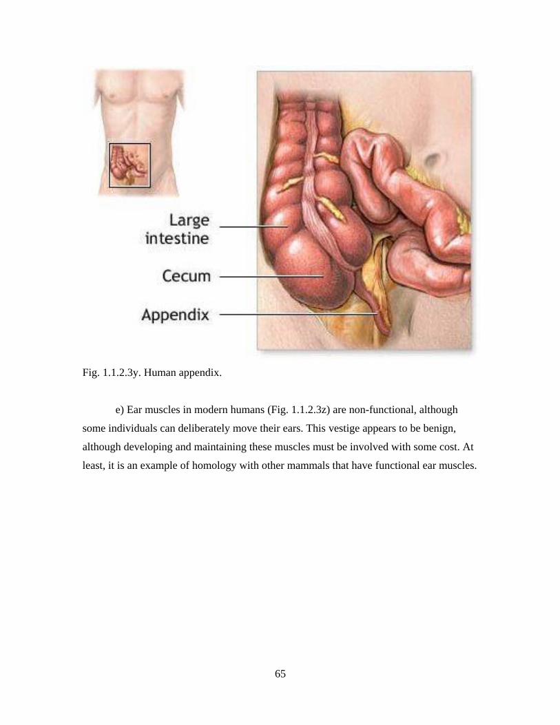
65

Fig. 1.1.2.3y. Human appendix.

e) Ear muscles in modern humans (Fig. 1.1.2.3z) are non-functional, although

some individuals can deliberately move their ears. This vestige appears to be benign,

although developing and maintaining these muscles must be involved with some cost. At

least, it is an example of homology with other mammals that have functional ear muscles.

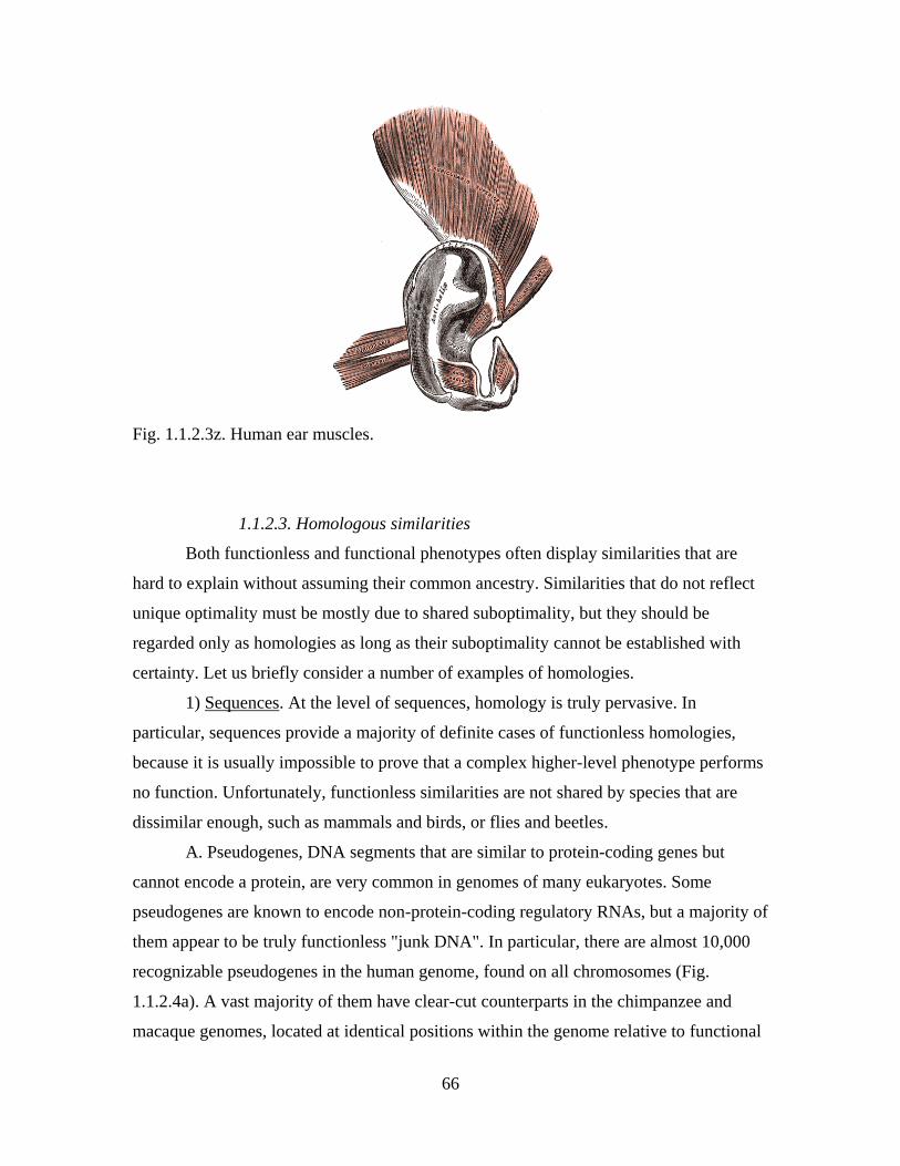
66

Fig. 1.1.2.3z. Human ear muscles.

1.1.2.3. Homologous similarities

Both functionless and functional phenotypes often display similarities that are

hard to explain without assuming their common ancestry. Similarities that do not reflect

unique optimality must be mostly due to shared suboptimality, but they should be

regarded only as homologies as long as their suboptimality cannot be established with

certainty. Let us briefly consider a number of examples of homologies.

1) Sequences. At the level of sequences, homology is truly pervasive. In

particular, sequences provide a majority of definite cases of functionless homologies,

because it is usually impossible to prove that a complex higher-level phenotype performs

no function. Unfortunately, functionless similarities are not shared by species that are

dissimilar enough, such as mammals and birds, or flies and beetles.

A. Pseudogenes, DNA segments that are similar to protein-coding genes but

cannot encode a protein, are very common in genomes of many eukaryotes. Some

pseudogenes are known to encode non-protein-coding regulatory RNAs, but a majority of

them appear to be truly functionless "junk DNA". In particular, there are almost 10,000

recognizable pseudogenes in the human genome, found on all chromosomes (Fig.

1.1.2.4a). A vast majority of them have clear-cut counterparts in the chimpanzee and

macaque genomes, located at identical positions within the genome relative to functional

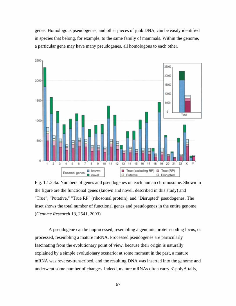
67

genes. Homologous pseudogenes, and other pieces of junk DNA, can be easily identified

in species that belong, for example, to the same family of mammals. Within the genome,

a particular gene may have many pseudogenes, all homologous to each other.

Fig. 1.1.2.4a. Numbers of genes and pseudogenes on each human chromosome. Shown in

the figure are the functional genes (known and novel, described in this study) and

"True", "Putative," "True RP" (ribosomal protein), and "Disrupted" pseudogenes. The

inset shows the total number of functional genes and pseudogenes in the entire genome

(Genome Research 13, 2541, 2003).

A pseudogene can be unprocessed, resembling a genomic protein-coding locus, or

processed, resembling a mature mRNA. Processed pseudogenes are particularly

fascinating from the evolutionary point of view, because their origin is naturally

explained by a simple evolutionary scenario: at some moment in the past, a mature

mRNA was reverse-transcribed, and the resulting DNA was inserted into the genome and

underwent some number of changes. Indeed, mature mRNAs often carry 3'-polyA tails,

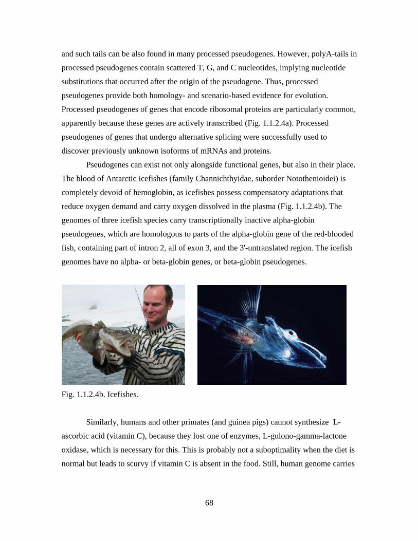
68

and such tails can be also found in many processed pseudogenes. However, polyA-tails in

processed pseudogenes contain scattered T, G, and C nucleotides, implying nucleotide

substitutions that occurred after the origin of the pseudogene. Thus, processed

pseudogenes provide both homology- and scenario-based evidence for evolution.

Processed pseudogenes of genes that encode ribosomal proteins are particularly common,

apparently because these genes are actively transcribed (Fig. 1.1.2.4a). Processed

pseudogenes of genes that undergo alternative splicing were successfully used to

discover previously unknown isoforms of mRNAs and proteins.

Pseudogenes can exist not only alongside functional genes, but also in their place.

The blood of Antarctic icefishes (family Channichthyidae, suborder Notothenioidei) is

completely devoid of hemoglobin, as icefishes possess compensatory adaptations that

reduce oxygen demand and carry oxygen dissolved in the plasma (Fig. 1.1.2.4b). The

genomes of three icefish species carry transcriptionally inactive alpha-globin

pseudogenes, which are homologous to parts of the alpha-globin gene of the red-blooded

fish, containing part of intron 2, all of exon 3, and the 3'-untranslated region. The icefish

genomes have no alpha- or beta-globin genes, or beta-globin pseudogenes.

Fig. 1.1.2.4b. Icefishes.

Similarly, humans and other primates (and guinea pigs) cannot synthesize L-

ascorbic acid (vitamin C), because they lost one of enzymes, L-gulono-gamma-lactone

oxidase, which is necessary for this. This is probably not a suboptimality when the diet is

normal but leads to scurvy if vitamin C is absent in the food. Still, human genome carries

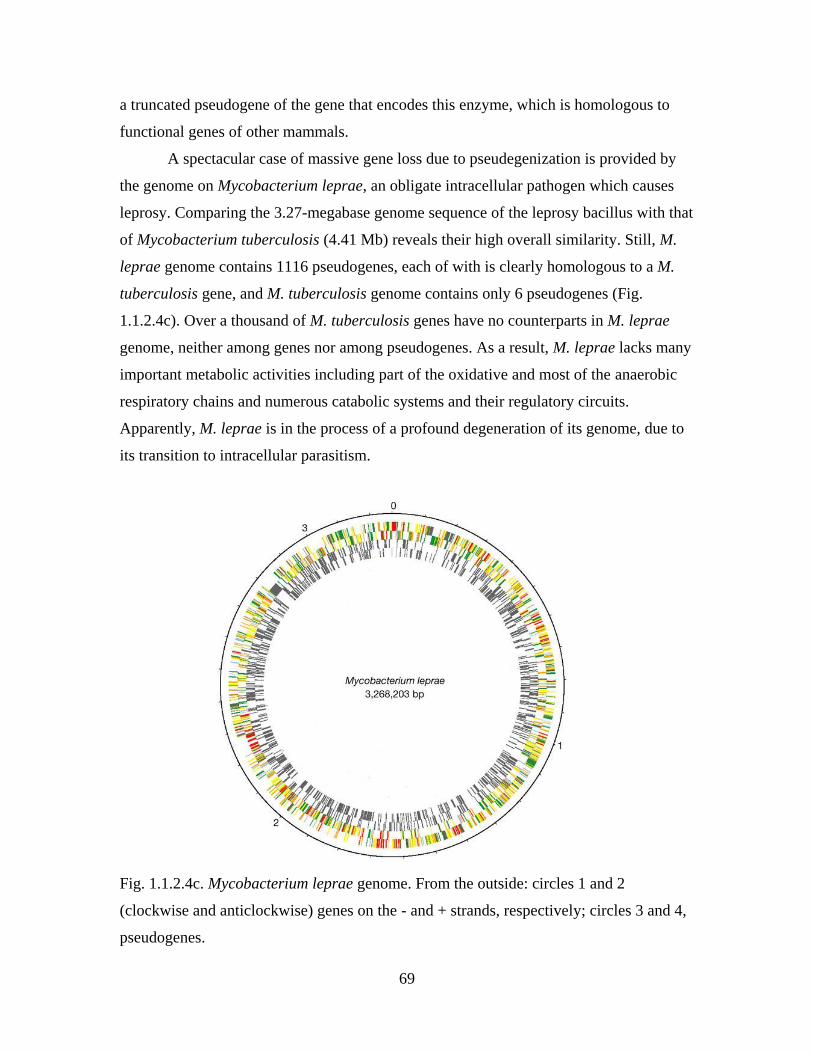
69

a truncated pseudogene of the gene that encodes this enzyme, which is homologous to

functional genes of other mammals.

A spectacular case of massive gene loss due to pseudegenization is provided by

the genome on Mycobacterium leprae, an obligate intracellular pathogen which causes

leprosy. Comparing the 3.27-megabase genome sequence of the leprosy bacillus with that

of Mycobacterium tuberculosis (4.41 Mb) reveals their high overall similarity. Still, M.

leprae genome contains 1116 pseudogenes, each of with is clearly homologous to a M.

tuberculosis gene, and M. tuberculosis genome contains only 6 pseudogenes (Fig.

1.1.2.4c). Over a thousand of M. tuberculosis genes have no counterparts in M. leprae

genome, neither among genes nor among pseudogenes. As a result, M. leprae lacks many

important metabolic activities including part of the oxidative and most of the anaerobic

respiratory chains and numerous catabolic systems and their regulatory circuits.

Apparently, M. leprae is in the process of a profound degeneration of its genome, due to

its transition to intracellular parasitism.

Fig. 1.1.2.4c. Mycobacterium leprae genome. From the outside: circles 1 and 2

(clockwise and anticlockwise) genes on the - and + strands, respectively; circles 3 and 4,

pseudogenes.

70

B. Transposable elements (TEs), DNA segments that have a propensity to insert

their copies into various locations of the genome, is another class of mostly junk DNA,

pervasive in many "bloated" genomes of eukaryotes. About 50% of the human genome

consist of recognizable TEs (Fig. 1.1.2.4d). As it is the case for pseudogenes, similar

species contain similar TE insertions at identical locations. Different families of human

TEs display different levels of divergence: on average, two MIR elements are ~30%

different from each other, and two Alu-repeats are only <10% different (Fig. 1.1.2.4d).

This pattern offer a scenario-based evidence for the Weak Claim for the human lineage,

because it can be naturally explained if we assume that MIR elements propagated in the

genome a long time ago, and Alu elements propagated more recently. Indeed, MIRs can

be found in genomes of all placental mammals, and Alu's are confined to primates.

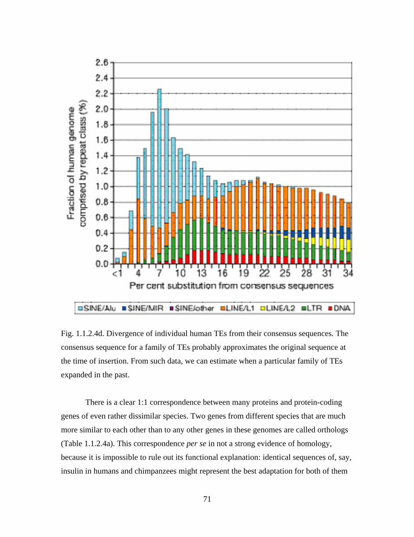
71

Fig. 1.1.2.4d. Divergence of individual human TEs from their consensus sequences. The

consensus sequence for a family of TEs probably approximates the original sequence at

the time of insertion. From such data, we can estimate when a particular family of TEs

expanded in the past.

There is a clear 1:1 correspondence between many proteins and protein-coding

genes of even rather dissimilar species. Two genes from different species that are much

more similar to each other than to any other genes in these genomes are called orthologs

(Table 1.1.2.4a). This correspondence per se in not a strong evidence of homology,

because it is impossible to rule out its functional explanation: identical sequences of, say,

insulin in humans and chimpanzees might represent the best adaptation for both of them

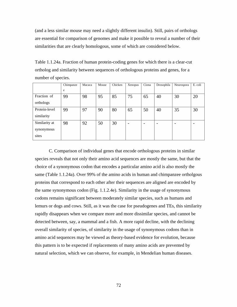
72

(and a less similar mouse may need a slightly different insulin). Still, pairs of orthologs

are essential for comparison of genomes and make it possible to reveal a number of their

similarities that are clearly homologous, some of which are considered below.

Table 1.1.24a. Fraction of human protein-coding genes for which there is a clear-cut

ortholog and similarity between sequences of orthologous proteins and genes, for a

number of species.

Chimpanze

e

Macaca Mouse Chicken Xenopus Ciona Drosophila Neurospora E. coli

Fraction of

orthologs

99 98 95 85 75 65 40 30 20

Protein-level

similarity

99 97 90 80 65 50 40 35 30

Similarity at

synonymous

sites

98 92 50 30 - - - - -

C. Comparison of individual genes that encode orthologous proteins in similar

species reveals that not only their amino acid sequences are mostly the same, but that the

choice of a synonymous codon that encodes a particular amino acid is also mostly the

same (Table 1.1.24a). Over 99% of the amino acids in human and chimpanzee ortholgous

proteins that correspond to each other after their sequences are aligned are encoded by

the same synonymous codon (Fig. 1.1.2.4e). Similarity in the usage of synonymous

codons remains significant between moderately similar species, such as humans and

lemurs or dogs and cows. Still, as it was the case for pseudogenes and TEs, this similarity

rapidly disappears when we compare more and more dissimilar species, and cannot be

detected between, say, a mammal and a fish. A more rapid decline, with the declining

overall similarity of species, of similarity in the usage of synonymous codons than in

amino acid sequences may be viewed as theory-based evidence for evolution, because

this pattern is to be expected if replacements of many amino acids are prevented by

natural selection, which we can observe, for example, in Mendelian human diseases.

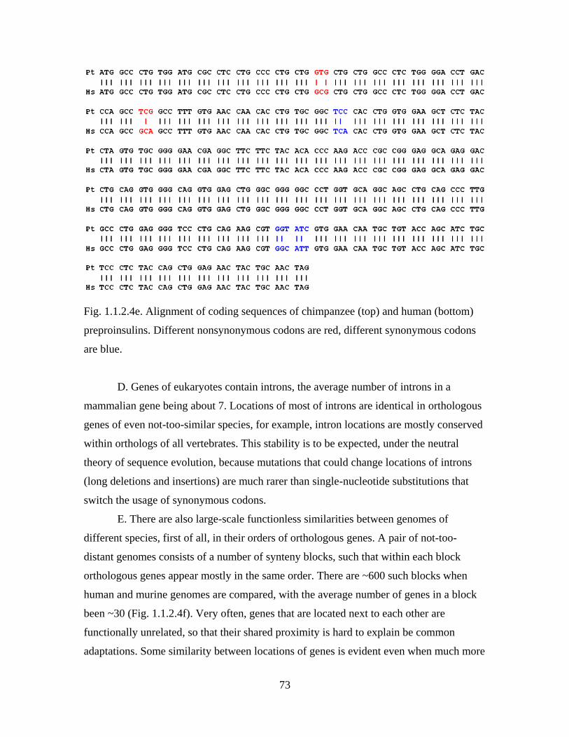
73

Fig. 1.1.2.4e. Alignment of coding sequences of chimpanzee (top) and human (bottom)

preproinsulins. Different nonsynonymous codons are red, different synonymous codons

are blue.

D. Genes of eukaryotes contain introns, the average number of introns in a

mammalian gene being about 7. Locations of most of introns are identical in orthologous

genes of even not-too-similar species, for example, intron locations are mostly conserved

within orthologs of all vertebrates. This stability is to be expected, under the neutral

theory of sequence evolution, because mutations that could change locations of introns

(long deletions and insertions) are much rarer than single-nucleotide substitutions that

switch the usage of synonymous codons.

E. There are also large-scale functionless similarities between genomes of

different species, first of all, in their orders of orthologous genes. A pair of not-too-

distant genomes consists of a number of synteny blocks, such that within each block

orthologous genes appear mostly in the same order. There are ~600 such blocks when

human and murine genomes are compared, with the average number of genes in a block

been ~30 (Fig. 1.1.2.4f). Very often, genes that are located next to each other are

functionally unrelated, so that their shared proximity is hard to explain be common

adaptations. Some similarity between locations of genes is evident even when much more

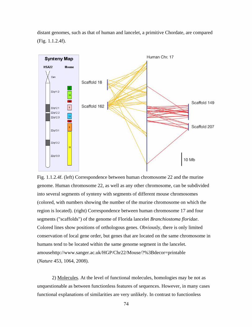
74

distant genomes, such as that of human and lancelet, a primitive Chordate, are compared

(Fig. 1.1.2.4f).

Fig. 1.1.2.4f. (left) Correspondence between human chromosome 22 and the murine

genome. Human chromosome 22, as well as any other chromosome, can be subdivided

into several segments of synteny with segments of different mouse chromosomes

(colored, with numbers showing the number of the murine chromosome on which the

region is located). (right) Correspondence between human chromosome 17 and four

segments ("scaffolds") of the genome of Florida lancelet Branchiostoma floridae.

Colored lines show positions of orthologous genes. Obviously, there is only limited

conservation of local gene order, but genes that are located on the same chromosome in

humans tend to be located within the same genome segment in the lancelet.

amousehttp://www.sanger.ac.uk/HGP/Chr22/Mouse/?%3Bdecor=printable

(Nature 453, 1064, 2008).

2) Molecules. At the level of functional molecules, homologies may be not as

unquestionable as between functionless features of sequences. However, in many cases

functional explanations of similarities are very unlikely. In contrast to functionless

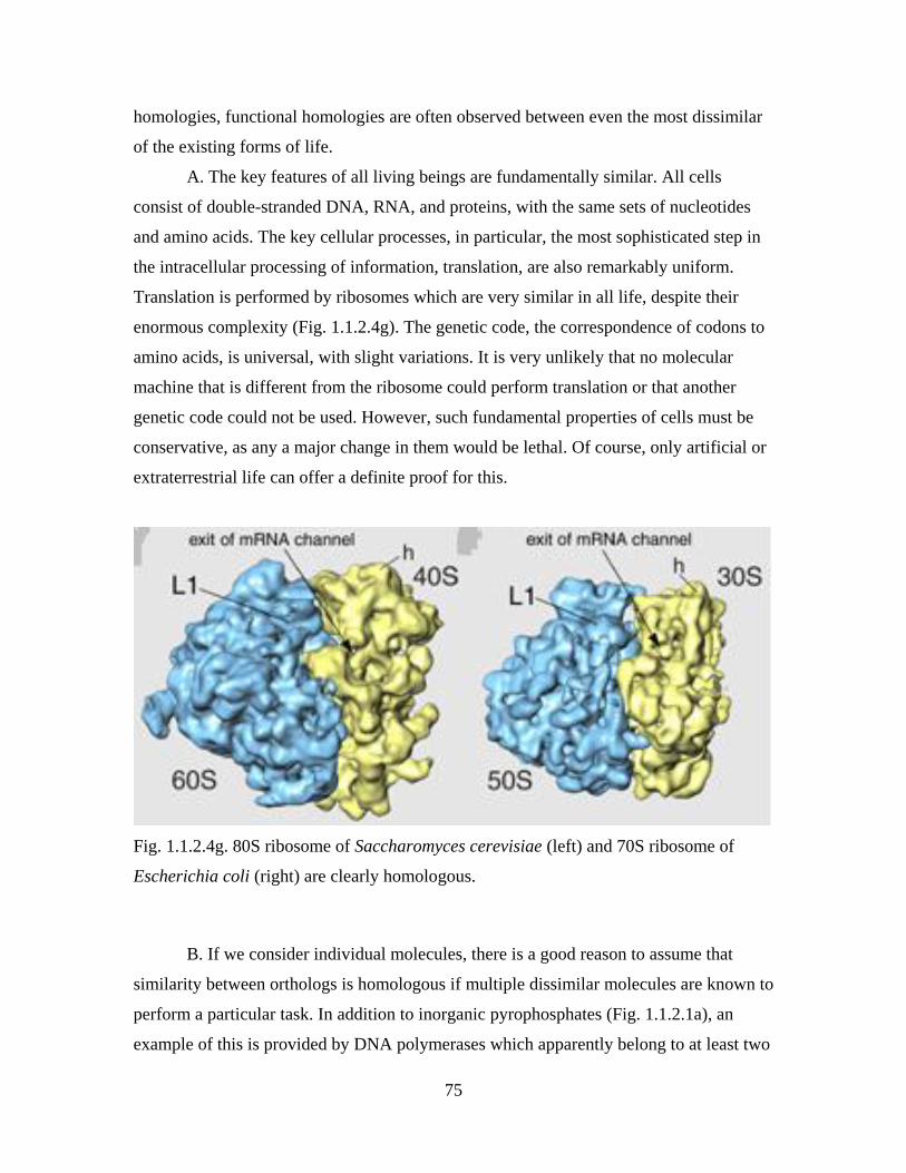
75

homologies, functional homologies are often observed between even the most dissimilar

of the existing forms of life.

A. The key features of all living beings are fundamentally similar. All cells

consist of double-stranded DNA, RNA, and proteins, with the same sets of nucleotides

and amino acids. The key cellular processes, in particular, the most sophisticated step in

the intracellular processing of information, translation, are also remarkably uniform.

Translation is performed by ribosomes which are very similar in all life, despite their

enormous complexity (Fig. 1.1.2.4g). The genetic code, the correspondence of codons to

amino acids, is universal, with slight variations. It is very unlikely that no molecular

machine that is different from the ribosome could perform translation or that another

genetic code could not be used. However, such fundamental properties of cells must be

conservative, as any a major change in them would be lethal. Of course, only artificial or

extraterrestrial life can offer a definite proof for this.

Fig. 1.1.2.4g. 80S ribosome of Saccharomyces cerevisiae (left) and 70S ribosome of

Escherichia coli (right) are clearly homologous.

B. If we consider individual molecules, there is a good reason to assume that

similarity between orthologs is homologous if multiple dissimilar molecules are known to

perform a particular task. In addition to inorganic pyrophosphates (Fig. 1.1.2.1a), an

example of this is provided by DNA polymerases which apparently belong to at least two

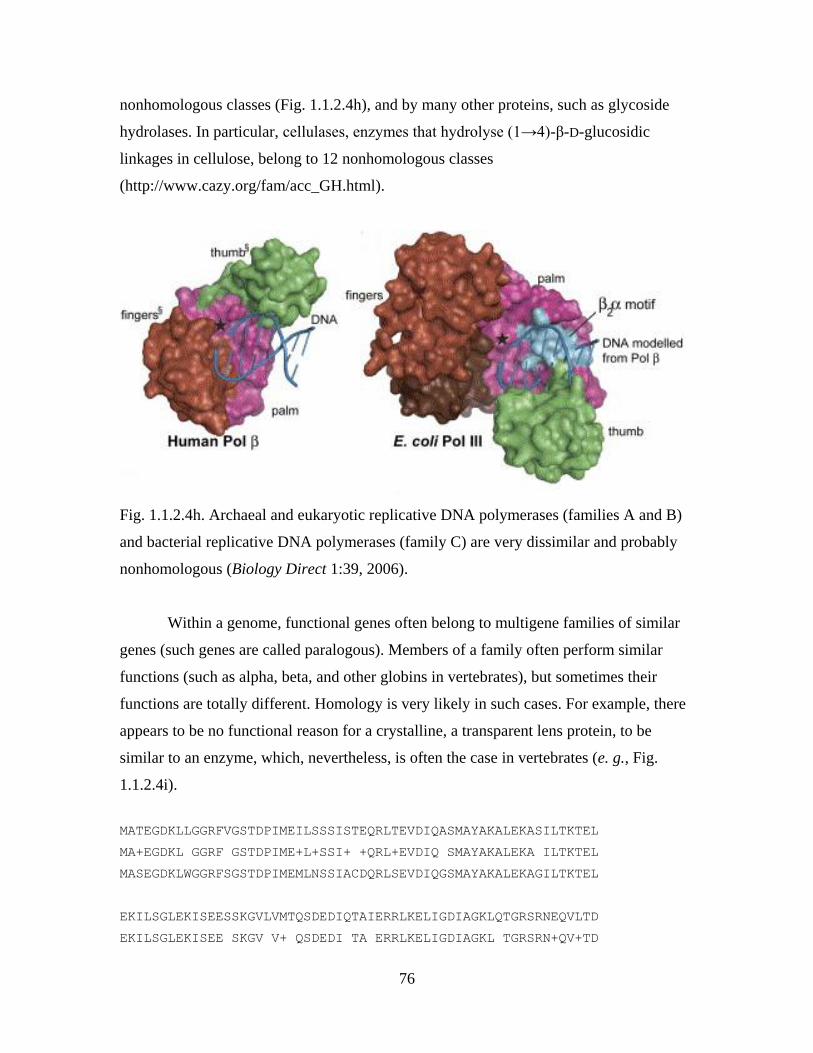
76

nonhomologous classes (Fig. 1.1.2.4h), and by many other proteins, such as glycoside

hydrolases. In particular, cellulases, enzymes that hydrolyse (1→4)-β-D-glucosidic

linkages in cellulose, belong to 12 nonhomologous classes

(http://www.cazy.org/fam/acc_GH.html).

Fig. 1.1.2.4h. Archaeal and eukaryotic replicative DNA polymerases (families A and B)

and bacterial replicative DNA polymerases (family C) are very dissimilar and probably

nonhomologous (Biology Direct 1:39, 2006).

Within a genome, functional genes often belong to multigene families of similar

genes (such genes are called paralogous). Members of a family often perform similar

functions (such as alpha, beta, and other globins in vertebrates), but sometimes their

functions are totally different. Homology is very likely in such cases. For example, there

appears to be no functional reason for a crystalline, a transparent lens protein, to be

similar to an enzyme, which, nevertheless, is often the case in vertebrates (e. g., Fig.

1.1.2.4i).

MATEGDKLLGGRFVGSTDPIMEILSSSISTEQRLTEVDIQASMAYAKALEKASILTKTEL

MA+EGDKL GGRF GSTDPIME+L+SSI+ +QRL+EVDIQ SMAYAKALEKA ILTKTEL

MASEGDKLWGGRFSGSTDPIMEMLNSSIACDQRLSEVDIQGSMAYAKALEKAGILTKTEL

EKILSGLEKISEESSKGVLVMTQSDEDIQTAIERRLKELIGDIAGKLQTGRSRNEQVLTD

EKILSGLEKISEE SKGV V+ QSDEDI TA ERRLKELIGDIAGKL TGRSRN+QV+TD

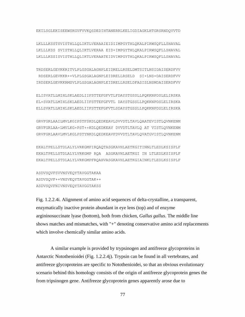
77

EKILSGLEKISEEWSKGVFVVKQSDEDIHTANERRLKELIGDIAGKLHTGRSRNDQVVTD

LKLLLKSSTSVISTHLLQLIKTLVERAAIEIDIIMPGYTHLQKALPIRWSQFLLSHAVAL

LKLLLKSS SVISTHLLQLIKTLVERAA EID+IMPGYTHLQKALPIRWSQFLLSHAVAL

LKLLLKSSISVISTHLLQLIKTLVERAATEIDVIMPGYTHLQKALPIRWSQFLLSHAVAL

TRDSERLGEVKKRITVLPLGSGALAGNPLEIDRELLRSELDMTSITLNSIDAISERDFVV

RDSERLGEVKKR++VLPLGSGALAGNPLEIDRELLRSELD SI+LNS+DAISERDFVV

IRDSERLGEVKKRMSVLPLGSGALAGNPLEIDRELLRSELDFASISLNSMDAISERDFVV

ELISVATLLMIHLSKLAEDLIIFSTTEFGFVTLFDAYSTGSSLLPQKKNPDSLELIRSKA

EL+SVATLLMIHLSKLAEDLIIFSTTEFGFVTL DAYSTGSSLLPQKKNPDSLELIRSKA

ELLSVATLLMIHLSKLAEDLIIFSTTEFGFVTLSDAYSTGSSLLPQKKNPDSLELIRSKA

GRVFGRLAAILMVLKGIPSTFSKDLQEDKEAVLDVVDTLTAVLQAATEVISTLQVNKENM

GRVFGRLAA+LMVLKG+PST++KDLQEDKEAV DVVDTLTAVLQ AT VISTLQVNKENM

GRVFGRLAAVLMVLKGLPSTYNKDLQEDKEAVFDVVDTLTAVLQVATGVISTLQVNKENM

EKALTPELLSTDLALYLVRKGMPIRQAQTASGKAVHLAETKGITINNLTLEDLKSISPLF

EKALTPELLSTDLALYLVRKGMP RQA ASGKAVHLAETKGI IN LTLEDLKSISPLF

EKALTPELLSTDLALYLVRKGMPFRQAHVASGKAVHLAETKGIAINKLTLEDLKSISPLF

ASDVSQVFSVVNSVEQYTAVGGTAKAA

ASDVSQVF++VNSVEQYTAVGGTAK++

ASDVSQVFNIVNSVEQYTAVGGTAKSS

Fig. 1.2.2.4i. Alignment of amino acid sequences of delta-crystalline, a transparent,

enzymatically inactive protein abundant in eye lens (top) and of enzyme

argininosuccinate lyase (bottom), both from chicken, Gallus gallus. The middle line

shows matches and mismatches, with "+" denoting conservative amino acid replacements

which involve chemically similar amino acids.

A similar example is provided by trypsinogen and antifreeze glycoproteins in

Antarctic Notothenioidei (Fig. 1.2.2.4j). Trypsin can be found in all vertebrates, and

antifreeze glycoproteins are specific to Notothenioidei, so that an obvious evolutionary

scenario behind this homology consists of the origin of antifreeze glycoprotein genes the

from tripsinogen gene. Antifreeze glycoprotein genes apparently arose due to

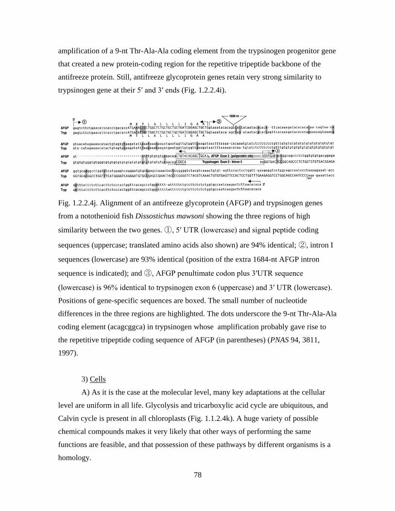
78

amplification of a 9-nt Thr-Ala-Ala coding element from the trypsinogen progenitor gene

that created a new protein-coding region for the repetitive tripeptide backbone of the

antifreeze protein. Still, antifreeze glycoprotein genes retain very strong similarity to

trypsinogen gene at their 5′ and 3′ ends (Fig. 1.2.2.4i).

Fig. 1.2.2.4j. Alignment of an antifreeze glycoprotein (AFGP) and trypsinogen genes

from a notothenioid fish Dissostichus mawsoni showing the three regions of high

similarity between the two genes. ①, 5′ UTR (lowercase) and signal peptide coding

sequences (uppercase; translated amino acids also shown) are 94% identical; ②, intron I

sequences (lowercase) are 93% identical (position of the extra 1684-nt AFGP intron

sequence is indicated); and ③, AFGP penultimate codon plus 3′UTR sequence

(lowercase) is 96% identical to trypsinogen exon 6 (uppercase) and 3′ UTR (lowercase).

Positions of gene-specific sequences are boxed. The small number of nucleotide

differences in the three regions are highlighted. The dots underscore the 9-nt Thr-Ala-Ala

coding element (acagcggca) in trypsinogen whose amplification probably gave rise to

the repetitive tripeptide coding sequence of AFGP (in parentheses) (PNAS 94, 3811,

1997).

3) Cells

A) As it is the case at the molecular level, many key adaptations at the cellular

level are uniform in all life. Glycolysis and tricarboxylic acid cycle are ubiquitous, and

Calvin cycle is present in all chloroplasts (Fig. 1.1.2.4k). A huge variety of possible

chemical compounds makes it very likely that other ways of performing the same

functions are feasible, and that possession of these pathways by different organisms is a

homology.

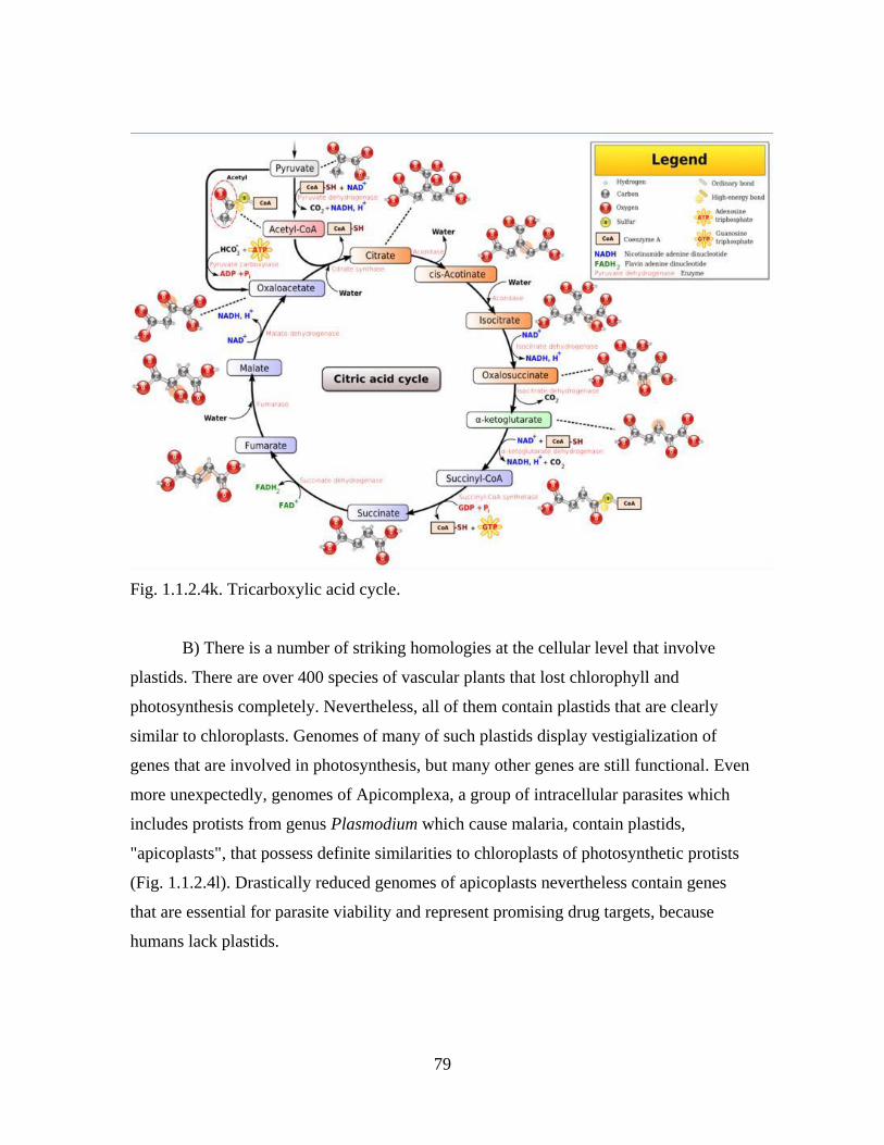
79

Fig. 1.1.2.4k. Tricarboxylic acid cycle.

B) There is a number of striking homologies at the cellular level that involve

plastids. There are over 400 species of vascular plants that lost chlorophyll and

photosynthesis completely. Nevertheless, all of them contain plastids that are clearly

similar to chloroplasts. Genomes of many of such plastids display vestigialization of

genes that are involved in photosynthesis, but many other genes are still functional. Even

more unexpectedly, genomes of Apicomplexa, a group of intracellular parasites which

includes protists from genus Plasmodium which cause malaria, contain plastids,

"apicoplasts", that possess definite similarities to chloroplasts of photosynthetic protists

(Fig. 1.1.2.4l). Drastically reduced genomes of apicoplasts nevertheless contain genes

that are essential for parasite viability and represent promising drug targets, because

humans lack plastids.

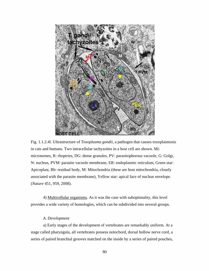
80

Fig. 1.1.2.4l. Ultrastructure of Toxoplasma gondii, a pathogen that causes toxoplasmosis

in cats and humans. Two intracellular tachyzoites in a host cell are shown. Mi:

micronemes, R: rhoptries, DG: dense granules, PV: parasitophorous vacuole, G: Golgi,

N: nucleus, PVM: parasite vacuole membrane, ER: endoplasmic reticulum, Green star:

Apicoplast, Rb: residual body, M: Mitochondria (these are host mitochondria, closely

associated with the parasite membrane), Yellow star: apical face of nuclear envelope.

(Nature 451, 959, 2008).

4) Multicellular organisms. As it was the case with suboptimality, this level

provides a wide variety of homologies, which can be subdivided into several groups.

A. Development

a) Early stages of the development of vertebrates are remarkably uniform. At a

stage called pharyngula, all vertebrates possess notochord, dorsal hollow nerve cord, a

series of paired branchial grooves matched on the inside by a series of paired pouches,

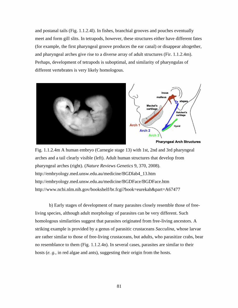
81

and postanal tails (Fig. 1.1.2.4l). In fishes, branchial grooves and pouches eventually

meet and form gill slits. In tetrapods, however, these structures either have different fates

(for example, the first pharyngeal groove produces the ear canal) or disappear altogether,

and pharyngeal arches give rise to a diverse array of adult structures (Fir. 1.1.2.4m).

Perhaps, development of tetrapods is suboptimal, and similarity of pharyngulas of

different vertebrates is very likely homologous.

Fig. 1.1.2.4m A human embryo (Carnegie stage 13) with 1st, 2nd and 3rd pharyngeal

arches and a tail clearly visible (left). Adult human structures that develop from

pharyngeal arches (right). (Nature Reviews Genetics 9, 370, 2008).

http://embryology.med.unsw.edu.au/medicine/BGDlab4_13.htm

http://embryology.med.unsw.edu.au/medicine/BGDFace/BGDFace.htm

http://www.ncbi.nlm.nih.gov/bookshelf/br.fcgi?book=eurekah&part=A67477

b) Early stages of development of many parasites closely resemble those of free-

living species, although adult morphology of parasites can be very different. Such

homologous similarities suggest that parasites originated from free-living ancestors. A

striking example is provided by a genus of parasitic crustaceans Sacculina, whose larvae

are rather similar to those of free-living crustaceans, but adults, who parasitize crabs, bear

no resemblance to them (Fig. 1.1.2.4n). In several cases, parasites are similar to their

hosts (e. g., in red algae and ants), suggesting their origin from the hosts.

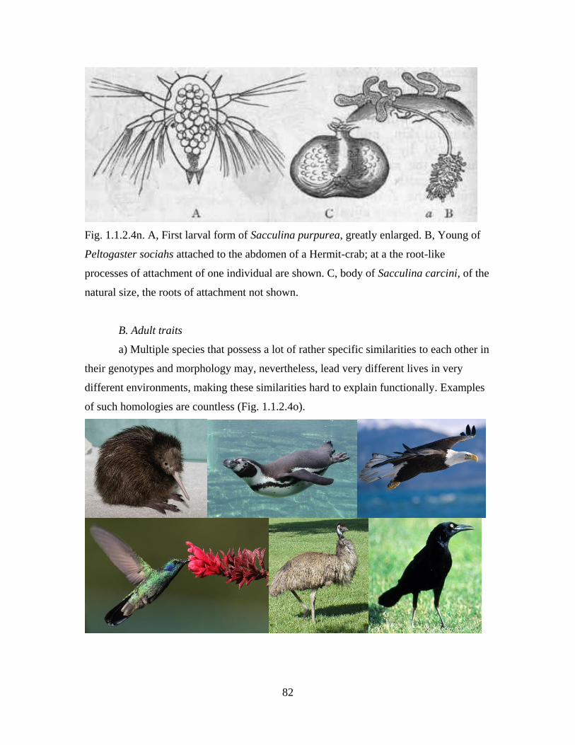
82

Fig. 1.1.2.4n. A, First larval form of Sacculina purpurea, greatly enlarged. B, Young of

Peltogaster sociahs attached to the abdomen of a Hermit-crab; at a the root-like

processes of attachment of one individual are shown. C, body of Sacculina carcini, of the

natural size, the roots of attachment not shown.

B. Adult traits

a) Multiple species that possess a lot of rather specific similarities to each other in

their genotypes and morphology may, nevertheless, lead very different lives in very

different environments, making these similarities hard to explain functionally. Examples

of such homologies are countless (Fig. 1.1.2.4o).

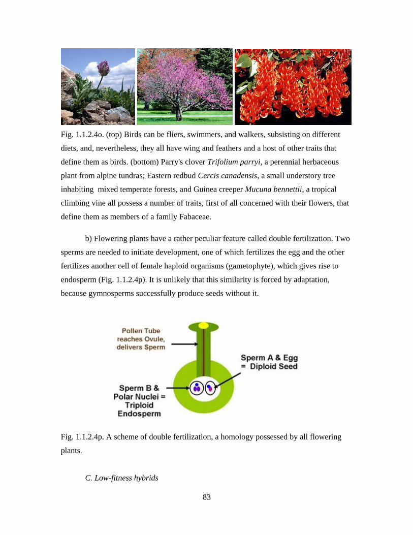
83

Fig. 1.1.2.4o. (top) Birds can be fliers, swimmers, and walkers, subsisting on different

diets, and, nevertheless, they all have wing and feathers and a host of other traits that

define them as birds. (bottom) Parry's clover Trifolium parryi, a perennial herbaceous

plant from alpine tundras; Eastern redbud Cercis canadensis, a small understory tree

inhabiting mixed temperate forests, and Guinea creeper Mucuna bennettii, a tropical

climbing vine all possess a number of traits, first of all concerned with their flowers, that

define them as members of a family Fabaceae.

b) Flowering plants have a rather peculiar feature called double fertilization. Two

sperms are needed to initiate development, one of which fertilizes the egg and the other

fertilizes another cell of female haploid organisms (gametophyte), which gives rise to

endosperm (Fig. 1.1.2.4p). It is unlikely that this similarity is forced by adaptation,

because gymnosperms successfully produce seeds without it.

Fig. 1.1.2.4p. A scheme of double fertilization, a homology possessed by all flowering

plants.

C. Low-fitness hybrids

84

Very many pairs of moderately similar forms of life can produce hybrids with

fitness reduced to various extents, from slight reduction of fertility of one sex only to rare

survival of weak and completely sterile offspring. Although low-fitness hybrids do not

demonstrate that the parental species are connected to each other, they reveal homology

of these species. Indeed, to produce a viable hybrid, even a severely impaired one, the

two parental species must be profoundly similar to each other (Fig. 1.1.2.4q).

Fig. 1.1.2.4q. A camel-llama hybrid.

D. Homologies revealed by intraspecies variation

Intraspecies variation involved in homologous similarity between species is a

separate, important class of homologies, and 3 subclasses should be recognized within it.

a) First, a rare variant within a species may be more similar than its normal

phenotype to normal phenotypes of another species. This fascinating phenomenon,

known as atavism, is particularly well-appreciated in humans, where even rare variants

may be recorded multiple times. A famous example of human atavism is provided by

vestigial tails (Fig. 1.1.2.4r). All humans has coccygeal vertebrae, homologous to

vertebrae in tails of mammals, which represent a more or less benign vestige,

homologous to such vertebrae in mammals that have tails. However, occasionally

humans develop, on the basis of the coccygeal vertebrae, vestigial tails, which are

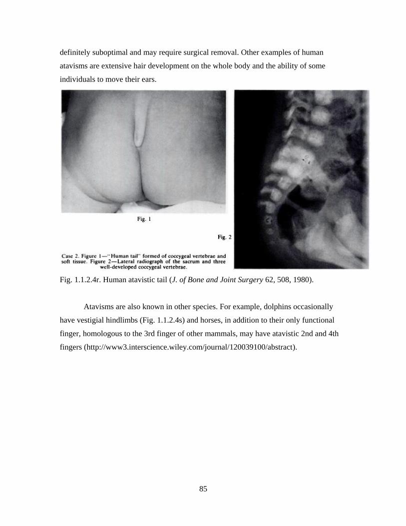
85

definitely suboptimal and may require surgical removal. Other examples of human

atavisms are extensive hair development on the whole body and the ability of some

individuals to move their ears.

Fig. 1.1.2.4r. Human atavistic tail (J. of Bone and Joint Surgery 62, 508, 1980).

Atavisms are also known in other species. For example, dolphins occasionally

have vestigial hindlimbs (Fig. 1.1.2.4s) and horses, in addition to their only functional

finger, homologous to the 3rd finger of other mammals, may have atavistic 2nd and 4th

fingers (http://www3.interscience.wiley.com/journal/120039100/abstract).

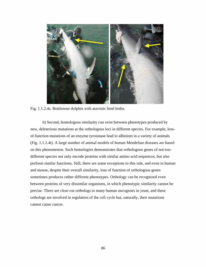
86

Fig. 1.1.2.4s. Bottlenose dolphin with atavistic hind limbs.

b) Second, homologous similarity can exist between phenotypes produced by

new, deleterious mutations at the orthologous loci in different species. For example, loss-

of-function mutations of an enzyme tyrosinase lead to albinism in a variety of animals

(Fig. 1.1.2.4t). A large number of animal models of human Mendelian diseases are based

on this phenomenon. Such homologies demonstrates that orthologous genes of not-too-

different species not only encode proteins with similar amino acid sequences, but also

perform similar functions. Still, there are some exceptions to this rule, and even in human

and mouse, despite their overall similarity, loss of function of orthologous genes

sometimes produces rather different phenotypes. Orthology can be recognized even

between proteins of very dissimilar organisms, in which phenotypic similarity cannot be

precise. There are clear-cut orthologs to many human oncogenes in yeast, and these

orthologs are involved in regulation of the cell cycle but, naturally, their mutations

cannot cause cancer.

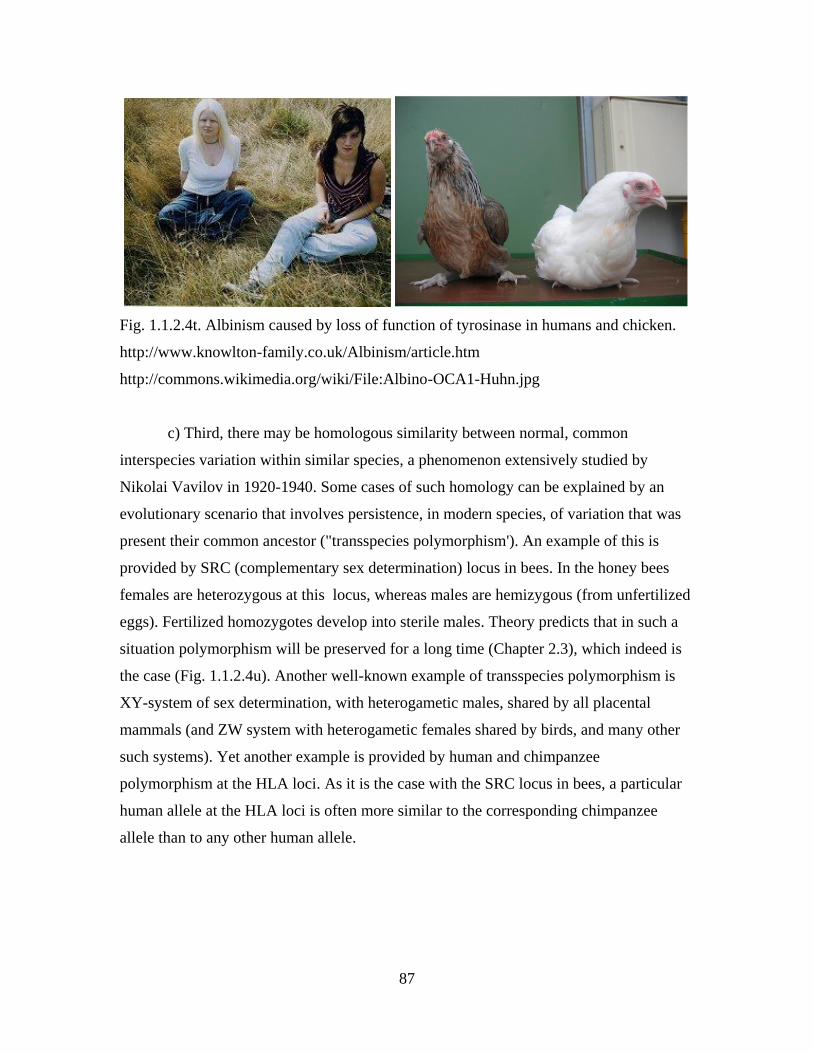
87

Fig. 1.1.2.4t. Albinism caused by loss of function of tyrosinase in humans and chicken.

http://www.knowlton-family.co.uk/Albinism/article.htm

http://commons.wikimedia.org/wiki/File:Albino-OCA1-Huhn.jpg

c) Third, there may be homologous similarity between normal, common

interspecies variation within similar species, a phenomenon extensively studied by

Nikolai Vavilov in 1920-1940. Some cases of such homology can be explained by an

evolutionary scenario that involves persistence, in modern species, of variation that was

present their common ancestor ("transspecies polymorphism'). An example of this is

provided by SRC (complementary sex determination) locus in bees. In the honey bees

females are heterozygous at this locus, whereas males are hemizygous (from unfertilized

eggs). Fertilized homozygotes develop into sterile males. Theory predicts that in such a

situation polymorphism will be preserved for a long time (Chapter 2.3), which indeed is

the case (Fig. 1.1.2.4u). Another well-known example of transspecies polymorphism is

XY-system of sex determination, with heterogametic males, shared by all placental

mammals (and ZW system with heterogametic females shared by birds, and many other

such systems). Yet another example is provided by human and chimpanzee

polymorphism at the HLA loci. As it is the case with the SRC locus in bees, a particular

human allele at the HLA loci is often more similar to the corresponding chimpanzee

allele than to any other human allele.

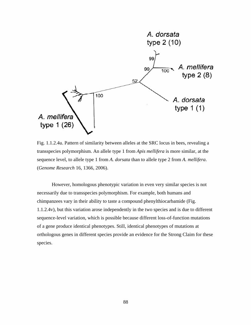
88

Fig. 1.1.2.4u. Pattern of similarity between alleles at the SRC locus in bees, revealing a

transspecies polymorphism. An allele type 1 from Apis mellifera is more similar, at the

sequence level, to allele type 1 from A. dorsata than to allele type 2 from A. mellifera.

(Genome Research 16, 1366, 2006).

However, homologous phenotypic variation in even very similar species is not

necessarily due to transspecies polymorphism. For example, both humans and

chimpanzees vary in their ability to taste a compound phenylthiocarbamide (Fig.

1.1.2.4v), but this variation arose independently in the two species and is due to different

sequence-level variation, which is possible because different loss-of-function mutations

of a gene produce identical phenotypes. Still, identical phenotypes of mutations at

orthologous genes in different species provide an evidence for the Strong Claim for these

species.

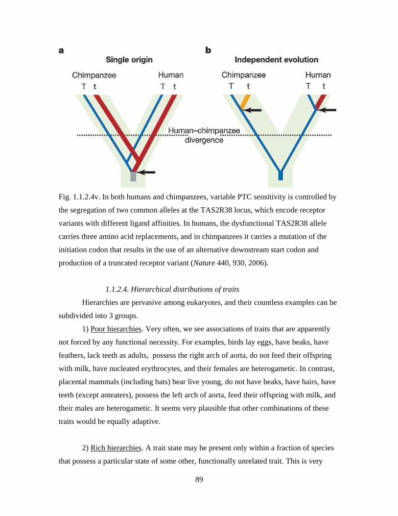
89

Fig. 1.1.2.4v. In both humans and chimpanzees, variable PTC sensitivity is controlled by

the segregation of two common alleles at the TAS2R38 locus, which encode receptor

variants with different ligand affinities. In humans, the dysfunctional TAS2R38 allele

carries three amino acid replacements, and in chimpanzees it carries a mutation of the

initiation codon that results in the use of an alternative downstream start codon and

production of a truncated receptor variant (Nature 440, 930, 2006).

1.1.2.4. Hierarchical distributions of traits

Hierarchies are pervasive among eukaryotes, and their countless examples can be

subdivided into 3 groups.

1) Poor hierarchies. Very often, we see associations of traits that are apparently

not forced by any functional necessity. For examples, birds lay eggs, have beaks, have

feathers, lack teeth as adults, possess the right arch of aorta, do not feed their offspring

with milk, have nucleated erythrocytes, and their females are heterogametic. In contrast,

placental mammals (including bats) bear live young, do not have beaks, have hairs, have

teeth (except anteaters), possess the left arch of aorta, feed their offspring with milk, and

their males are heterogametic. It seems very plausible that other combinations of these

traits would be equally adaptive.

2) Rich hierarchies. A trait state may be present only within a fraction of species

that possess a particular state of some other, functionally unrelated trait. This is very

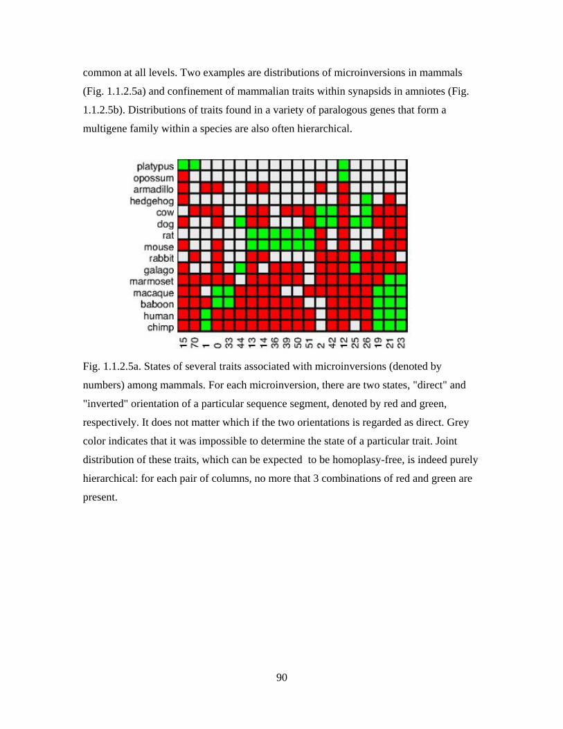
90

common at all levels. Two examples are distributions of microinversions in mammals

(Fig. 1.1.2.5a) and confinement of mammalian traits within synapsids in amniotes (Fig.

1.1.2.5b). Distributions of traits found in a variety of paralogous genes that form a

multigene family within a species are also often hierarchical.

Fig. 1.1.2.5a. States of several traits associated with microinversions (denoted by

numbers) among mammals. For each microinversion, there are two states, "direct" and

"inverted" orientation of a particular sequence segment, denoted by red and green,

respectively. It does not matter which if the two orientations is regarded as direct. Grey

color indicates that it was impossible to determine the state of a particular trait. Joint

distribution of these traits, which can be expected to be homoplasy-free, is indeed purely

hierarchical: for each pair of columns, no more that 3 combinations of red and green are

present.

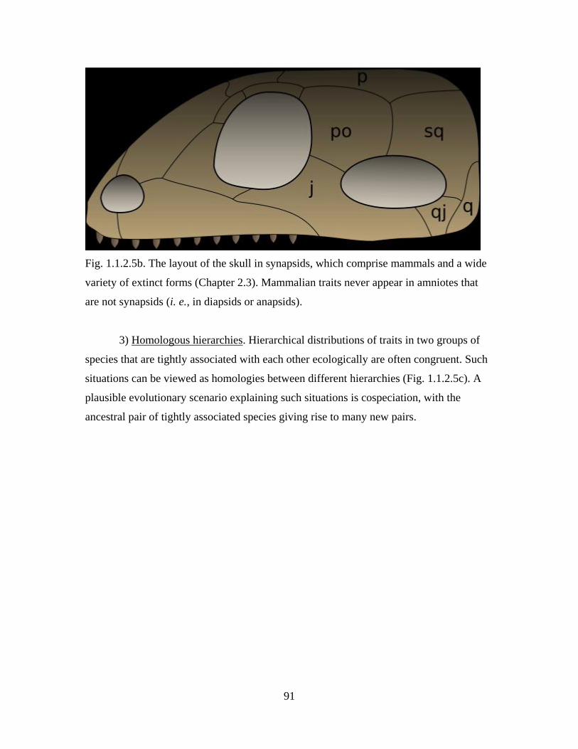
91

Fig. 1.1.2.5b. The layout of the skull in synapsids, which comprise mammals and a wide

variety of extinct forms (Chapter 2.3). Mammalian traits never appear in amniotes that

are not synapsids (i. e., in diapsids or anapsids).

3) Homologous hierarchies. Hierarchical distributions of traits in two groups of

species that are tightly associated with each other ecologically are often congruent. Such

situations can be viewed as homologies between different hierarchies (Fig. 1.1.2.5c). A

plausible evolutionary scenario explaining such situations is cospeciation, with the

ancestral pair of tightly associated species giving rise to many new pairs.

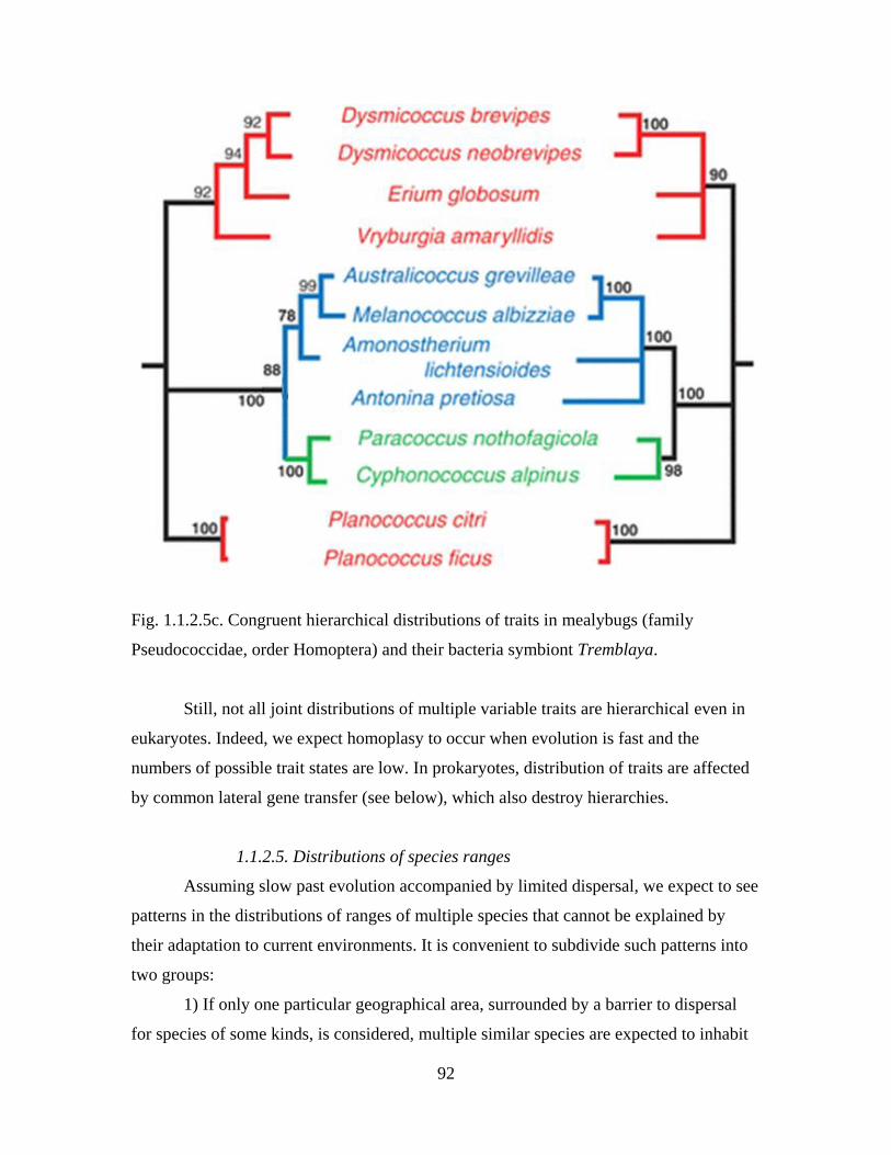
92

Fig. 1.1.2.5c. Congruent hierarchical distributions of traits in mealybugs (family

Pseudococcidae, order Homoptera) and their bacteria symbiont Tremblaya.

Still, not all joint distributions of multiple variable traits are hierarchical even in

eukaryotes. Indeed, we expect homoplasy to occur when evolution is fast and the

numbers of possible trait states are low. In prokaryotes, distribution of traits are affected

by common lateral gene transfer (see below), which also destroy hierarchies.

1.1.2.5. Distributions of species ranges

Assuming slow past evolution accompanied by limited dispersal, we expect to see

patterns in the distributions of ranges of multiple species that cannot be explained by

their adaptation to current environments. It is convenient to subdivide such patterns into

two groups:

1) If only one particular geographical area, surrounded by a barrier to dispersal

for species of some kinds, is considered, multiple similar species are expected to inhabit

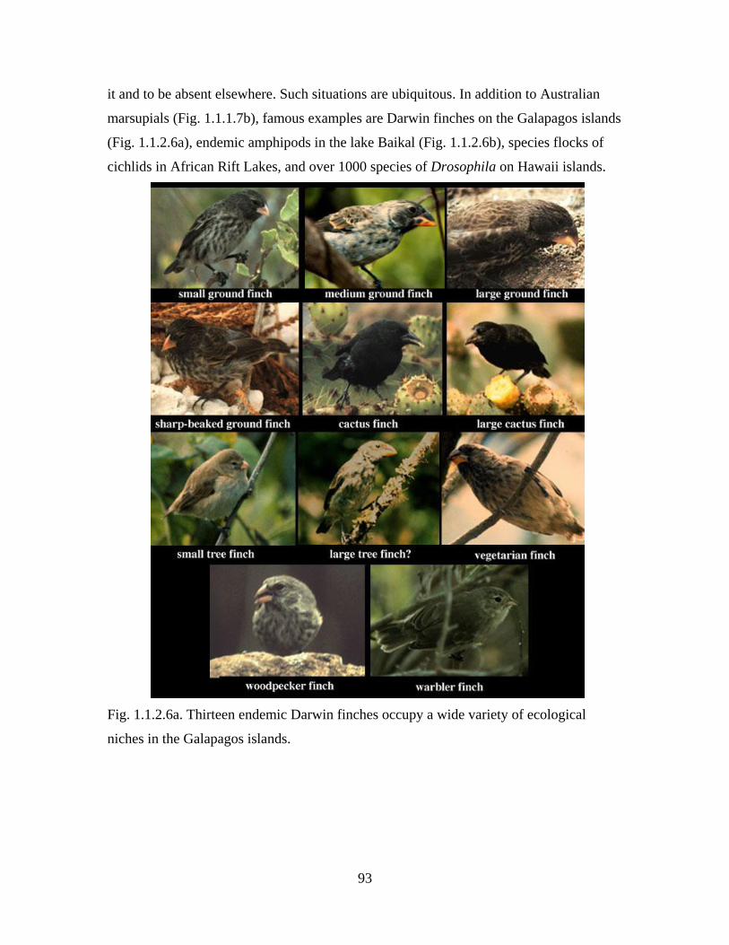
93

it and to be absent elsewhere. Such situations are ubiquitous. In addition to Australian

marsupials (Fig. 1.1.1.7b), famous examples are Darwin finches on the Galapagos islands

(Fig. 1.1.2.6a), endemic amphipods in the lake Baikal (Fig. 1.1.2.6b), species flocks of

cichlids in African Rift Lakes, and over 1000 species of Drosophila on Hawaii islands.

Fig. 1.1.2.6a. Thirteen endemic Darwin finches occupy a wide variety of ecological

niches in the Galapagos islands.

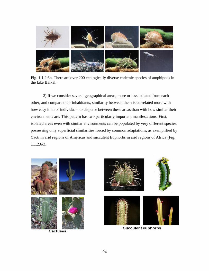
94

Fig. 1.1.2.6b. There are over 200 ecologically diverse endemic species of amphipods in the lake Baikal.

2) If we consider several geographical areas, more or less isolated from each

other, and compare their inhabitants, similarity between them is correlated more with

how easy it is for individuals to disperse between these areas than with how similar their

environments are. This pattern has two particularly important manifestations. First,

isolated areas even with similar environments can be populated by very different species,

possessing only superficial similarities forced by common adaptations, as exemplified by

Cacti in arid regions of Americas and succulent Euphorbs in arid regions of Africa (Fig.

1.1.2.6c).

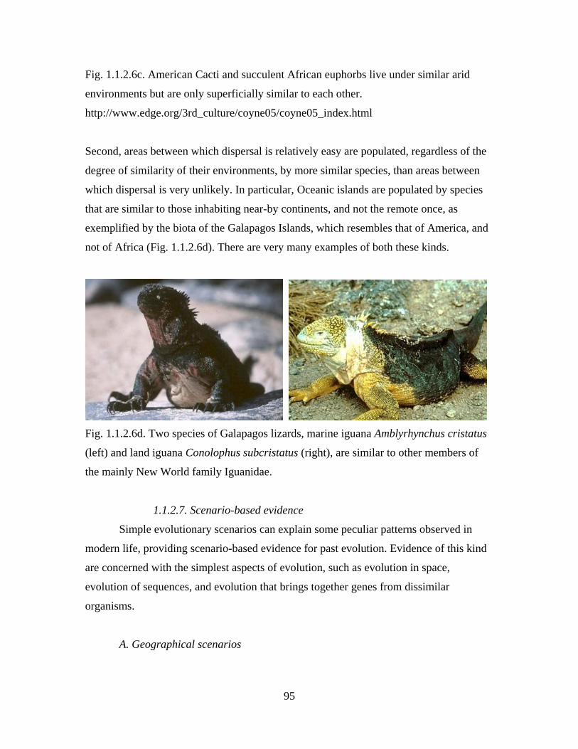
95

Fig. 1.1.2.6c. American Cacti and succulent African euphorbs live under similar arid

environments but are only superficially similar to each other.

http://www.edge.org/3rd_culture/coyne05/coyne05_index.html

Second, areas between which dispersal is relatively easy are populated, regardless of the

degree of similarity of their environments, by more similar species, than areas between

which dispersal is very unlikely. In particular, Oceanic islands are populated by species

that are similar to those inhabiting near-by continents, and not the remote once, as

exemplified by the biota of the Galapagos Islands, which resembles that of America, and

not of Africa (Fig. 1.1.2.6d). There are very many examples of both these kinds.

Fig. 1.1.2.6d. Two species of Galapagos lizards, marine iguana Amblyrhynchus cristatus

(left) and land iguana Conolophus subcristatus (right), are similar to other members of

the mainly New World family Iguanidae.

1.1.2.7. Scenario-based evidence

Simple evolutionary scenarios can explain some peculiar patterns observed in

modern life, providing scenario-based evidence for past evolution. Evidence of this kind

are concerned with the simplest aspects of evolution, such as evolution in space,

evolution of sequences, and evolution that brings together genes from dissimilar

organisms.

A. Geographical scenarios

96

There are indirect evidence for evolution based on distribution of species in space

that go beyond a simple assumption of limited dispersal, and, in addition, assume a

particular scenario of geological changes in the past. Let us consider two examples.

a) Suppose that in the past a previously continuous area (either a continent or an

ocean) split into two, triggering independent evolution of now-isolated parts of a lineage

and their progressive divergence, a scenario known as vicariance. Thus, after a long

enough time elapsed since the split, we can expect to observe many pairs of similar

species in the two now-separated areas. A striking example of this pattern is provided by

transithmean species pairs of many marine organisms, inhabiting the Caribbean and the

Pacific. Indeed, for a Caribbean species the most similar species is usually found on the

other side of the Isthmus of Panama, in the Pacific (and vice versa) (Fig. 1.1.2.7a). This

pattern provides evidence both for the common ancestry of each transithmean species

pair and for a relatively recent separation of the Caribbean from the Pacific which,

according to the geological data, occurred ~5Mya.

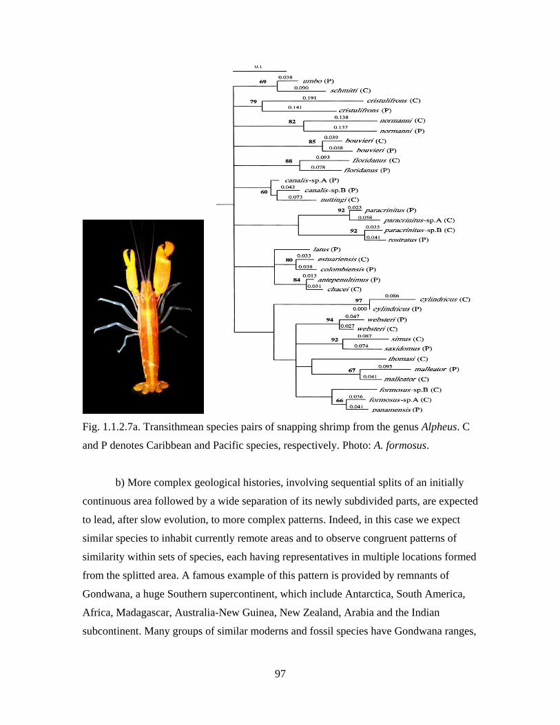
97

Fig. 1.1.2.7a. Transithmean species pairs of snapping shrimp from the genus Alpheus. C

and P denotes Caribbean and Pacific species, respectively. Photo: A. formosus.

b) More complex geological histories, involving sequential splits of an initially

continuous area followed by a wide separation of its newly subdivided parts, are expected

to lead, after slow evolution, to more complex patterns. Indeed, in this case we expect

similar species to inhabit currently remote areas and to observe congruent patterns of

similarity within sets of species, each having representatives in multiple locations formed

from the splitted area. A famous example of this pattern is provided by remnants of

Gondwana, a huge Southern supercontinent, which include Antarctica, South America,

Africa, Madagascar, Australia-New Guinea, New Zealand, Arabia and the Indian

subcontinent. Many groups of similar moderns and fossil species have Gondwana ranges,

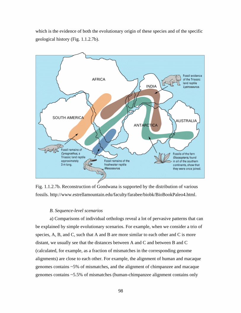
98

which is the evidence of both the evolutionary origin of these species and of the specific

geological history (Fig. 1.1.2.7b).

Fig. 1.1.2.7b. Reconstruction of Gondwana is supported by the distribution of various

fossils. http://www.estrellamountain.edu/faculty/farabee/biobk/BioBookPaleo4.html.

B. Sequence-level scenarios

a) Comparisons of individual orthologs reveal a lot of pervasive patterns that can

be explained by simple evolutionary scenarios. For example, when we consider a trio of

species, A, B, and C, such that A and B are more similar to each other and C is more

distant, we usually see that the distances between A and C and between B and C

(calculated, for example, as a fraction of mismatches in the corresponding genome

alignments) are close to each other. For example, the alignment of human and macaque

genomes contains ~5% of mismatches, and the alignment of chimpanzee and macaque

genomes contains ~5.5% of mismatches (human-chimpanzee alignment contains only

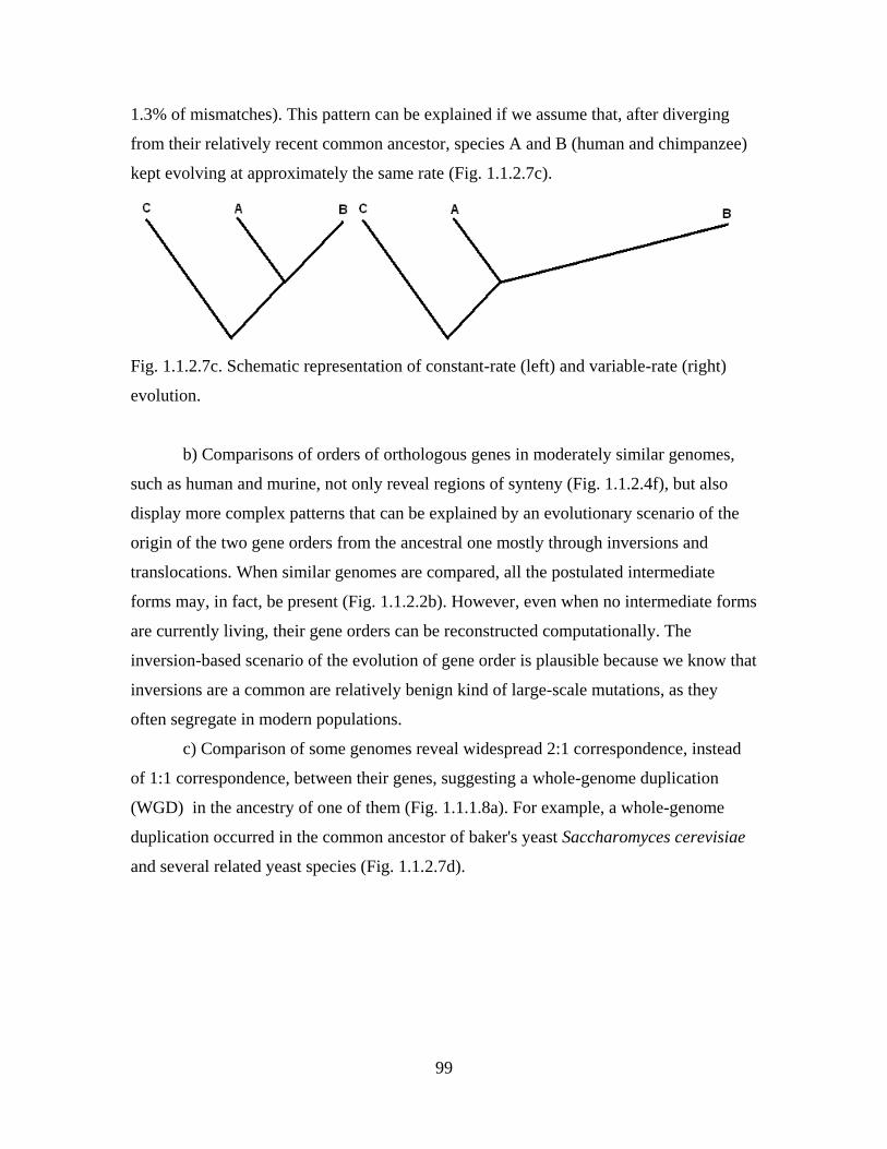
99

1.3% of mismatches). This pattern can be explained if we assume that, after diverging

from their relatively recent common ancestor, species A and B (human and chimpanzee)

kept evolving at approximately the same rate (Fig. 1.1.2.7c).

Fig. 1.1.2.7c. Schematic representation of constant-rate (left) and variable-rate (right)

evolution.

b) Comparisons of orders of orthologous genes in moderately similar genomes,

such as human and murine, not only reveal regions of synteny (Fig. 1.1.2.4f), but also

display more complex patterns that can be explained by an evolutionary scenario of the

origin of the two gene orders from the ancestral one mostly through inversions and

translocations. When similar genomes are compared, all the postulated intermediate

forms may, in fact, be present (Fig. 1.1.2.2b). However, even when no intermediate forms

are currently living, their gene orders can be reconstructed computationally. The

inversion-based scenario of the evolution of gene order is plausible because we know that

inversions are a common are relatively benign kind of large-scale mutations, as they

often segregate in modern populations.

c) Comparison of some genomes reveal widespread 2:1 correspondence, instead

of 1:1 correspondence, between their genes, suggesting a whole-genome duplication

(WGD) in the ancestry of one of them (Fig. 1.1.1.8a). For example, a whole-genome

duplication occurred in the common ancestor of baker's yeast Saccharomyces cerevisiae

and several related yeast species (Fig. 1.1.2.7d).

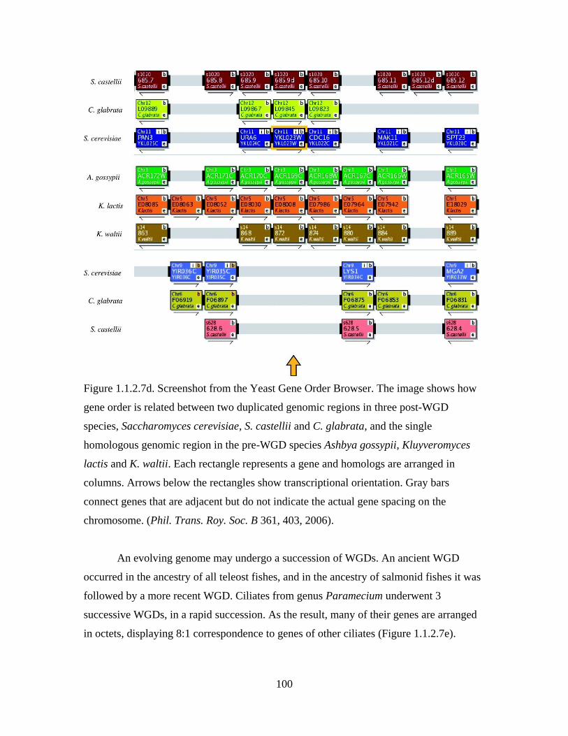
100

Figure 1.1.2.7d. Screenshot from the Yeast Gene Order Browser. The image shows how

gene order is related between two duplicated genomic regions in three post-WGD

species, Saccharomyces cerevisiae, S. castellii and C. glabrata, and the single

homologous genomic region in the pre-WGD species Ashbya gossypii, Kluyveromyces

lactis and K. waltii. Each rectangle represents a gene and homologs are arranged in

columns. Arrows below the rectangles show transcriptional orientation. Gray bars

connect genes that are adjacent but do not indicate the actual gene spacing on the

chromosome. (Phil. Trans. Roy. Soc. B 361, 403, 2006).

An evolving genome may undergo a succession of WGDs. An ancient WGD

occurred in the ancestry of all teleost fishes, and in the ancestry of salmonid fishes it was

followed by a more recent WGD. Ciliates from genus Paramecium underwent 3

successive WGDs, in a rapid succession. As the result, many of their genes are arranged

in octets, displaying 8:1 correspondence to genes of other ciliates (Figure 1.1.2.7e).

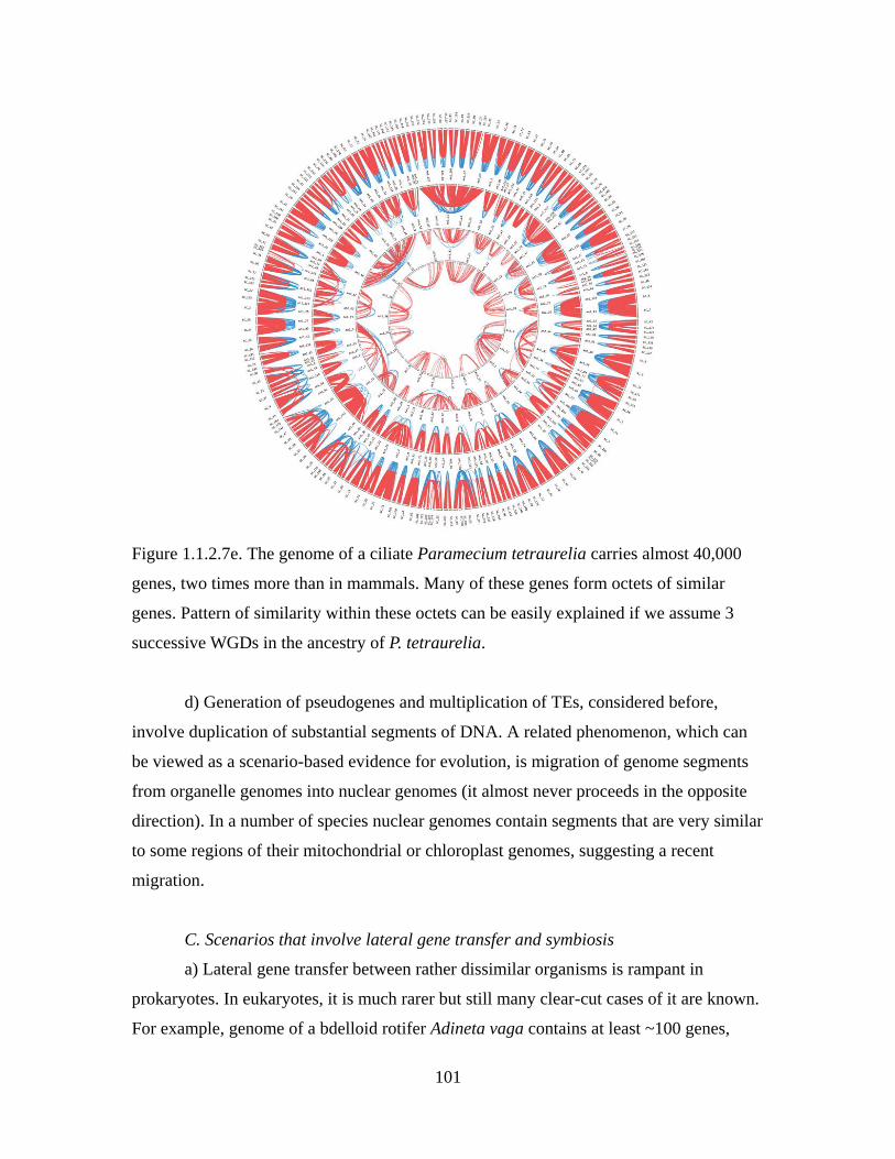
101

Figure 1.1.2.7e. The genome of a ciliate Paramecium tetraurelia carries almost 40,000

genes, two times more than in mammals. Many of these genes form octets of similar

genes. Pattern of similarity within these octets can be easily explained if we assume 3

successive WGDs in the ancestry of P. tetraurelia.

d) Generation of pseudogenes and multiplication of TEs, considered before,

involve duplication of substantial segments of DNA. A related phenomenon, which can

be viewed as a scenario-based evidence for evolution, is migration of genome segments

from organelle genomes into nuclear genomes (it almost never proceeds in the opposite

direction). In a number of species nuclear genomes contain segments that are very similar

to some regions of their mitochondrial or chloroplast genomes, suggesting a recent

migration.

C. Scenarios that involve lateral gene transfer and symbiosis

a) Lateral gene transfer between rather dissimilar organisms is rampant in

prokaryotes. In eukaryotes, it is much rarer but still many clear-cut cases of it are known.

For example, genome of a bdelloid rotifer Adineta vaga contains at least ~100 genes,

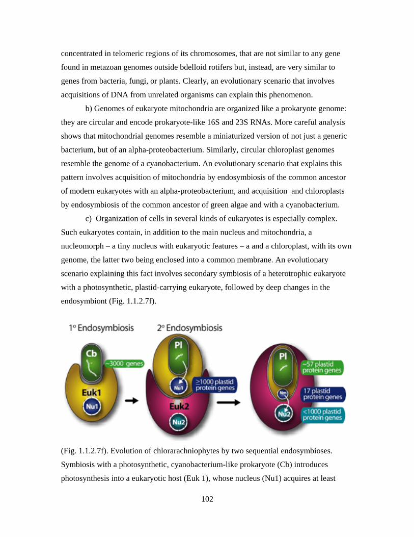
102

concentrated in telomeric regions of its chromosomes, that are not similar to any gene

found in metazoan genomes outside bdelloid rotifers but, instead, are very similar to

genes from bacteria, fungi, or plants. Clearly, an evolutionary scenario that involves

acquisitions of DNA from unrelated organisms can explain this phenomenon.

b) Genomes of eukaryote mitochondria are organized like a prokaryote genome:

they are circular and encode prokaryote-like 16S and 23S RNAs. More careful analysis

shows that mitochondrial genomes resemble a miniaturized version of not just a generic

bacterium, but of an alpha-proteobacterium. Similarly, circular chloroplast genomes

resemble the genome of a cyanobacterium. An evolutionary scenario that explains this

pattern involves acquisition of mitochondria by endosymbiosis of the common ancestor

of modern eukaryotes with an alpha-proteobacterium, and acquisition and chloroplasts

by endosymbiosis of the common ancestor of green algae and with a cyanobacterium.

c) Organization of cells in several kinds of eukaryotes is especially complex.

Such eukaryotes contain, in addition to the main nucleus and mitochondria, a

nucleomorph – a tiny nucleus with eukaryotic features – a and a chloroplast, with its own

genome, the latter two being enclosed into a common membrane. An evolutionary

scenario explaining this fact involves secondary symbiosis of a heterotrophic eukaryote

with a photosynthetic, plastid-carrying eukaryote, followed by deep changes in the

endosymbiont (Fig. 1.1.2.7f).

(Fig. 1.1.2.7f). Evolution of chlorarachniophytes by two sequential endosymbioses.

Symbiosis with a photosynthetic, cyanobacterium-like prokaryote (Cb) introduces

photosynthesis into a eukaryotic host (Euk 1), whose nucleus (Nu1) acquires at least

103

1,000 cyanobacterial genes over time. Secondary endosymbiosis involves capture and

retention of the primary photosynthetic eukaryote by another eukaryote (Euk 2),

producing a plastid with four bounding membranes. Essential plastid protein genes are

transferred from the endosymbiont nucleus (Nm, nucleomorph) to the nucleus (Nu2) of

the second eukaryotic host (PNAS 103, 9566, 2006).

1.1.2.8. Theory-based evidence

Although we still lack a comprehensive theory of evolution, progress of the last

decades produced a number of partial theories that can describe some of the simplest

aspects of this process. Thus, there is a number of situations, where theoretical

predictions can be compared with the data. It will be more convenient, however, to treat

most of such situations in Part 3. Here I present just two more examples of theory-based

evidence.

a) We already encountered the neutral theory of sequence evolution, which

predicts that the rate of evolution of a functionless segment of a sequence must be equal

to the mutation rate. One prediction of this theory is that relative abundances of

substitutions of different kinds within a segment of DNA is the same as relative

abundances of mutations (Fig. 1.1.1.8c). Another prediction is that different segments of

functionless DNA within the genome must evolve at similar rates, as long as the mutation

rate is approximately uniform across the genome. This is, indeed, the case: divergence at

more or less selectively neutral DNA sites between a pair is moderately similar genomes

is approximately the same throughout the whole genome (Fig. 1.1.2.8a).

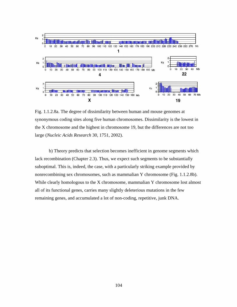
104

Fig. 1.1.2.8a. The degree of dissimilarity between human and mouse genomes at

synonymous coding sites along five human chromosomes. Dissimilarity is the lowest in

the X chromosome and the highest in chromosome 19, but the differences are not too

large (Nucleic Acids Research 30, 1751, 2002).

b) Theory predicts that selection becomes inefficient in genome segments which

lack recombination (Chapter 2.3). Thus, we expect such segments to be substantially

suboptimal. This is, indeed, the case, with a particularly striking example provided by

nonrecombining sex chromosomes, such as mammalian Y chromosome (Fig. 1.1.2.8b).

While clearly homologous to the X chromosome, mammalian Y chromosome lost almost

all of its functional genes, carries many slightly deleterious mutations in the few

remaining genes, and accumulated a lot of non-coding, repetitive, junk DNA.

105

Fig. 1.1.2.8b. Mammalian X and Y chromosome.

1.1.2.8. Past evolution of life is a fact

Indirect evidence for past evolution, a sample of which we just reviewed, support

the Weak Claim for each individuals species ever studied and the Strong Claim for the

whole diversity of modern life. Direct evidence, provided by fossils, tell the same story

(Chapters 1.2 and 1.3). There are more known traces of past evolution of life than of any

other past event or process, studied by any natural science. Indeed, life in which all

adaptations are perfect, all similarities between phenotypes and geographical ranges of

different species are forced by similarities of their adaptations, all hierarchical

distributions of traits are forced by low fitness of absent combinations of trait states, etc.,

would be a totally unfamiliar sight. Thus, evolutionary origin of modern life is an

established fact.

Of course, an omnipotent supernatural Creator, or incredibly advanced space

aliens, could do a perfect job imitating the outcome of natural evolution, and making sure

that, after each species has been created independently "as is", some species have

vestigial eyes, humans and chimpanzees share thousands of processed pseudogenes,

horses and donkeys are compatible enough to produce viable mules, all birds have wings,

feathers and the right arch of aorta, hundreds of endemic species of cichlids live in lake

Malawi, and genomes of mitochondria look like a reduced genome of an alpha-

proteobacterium. However, admitting such explanations of data would make any study of

nature impossible. Refusal by some people to accept facts is an interesting sociological

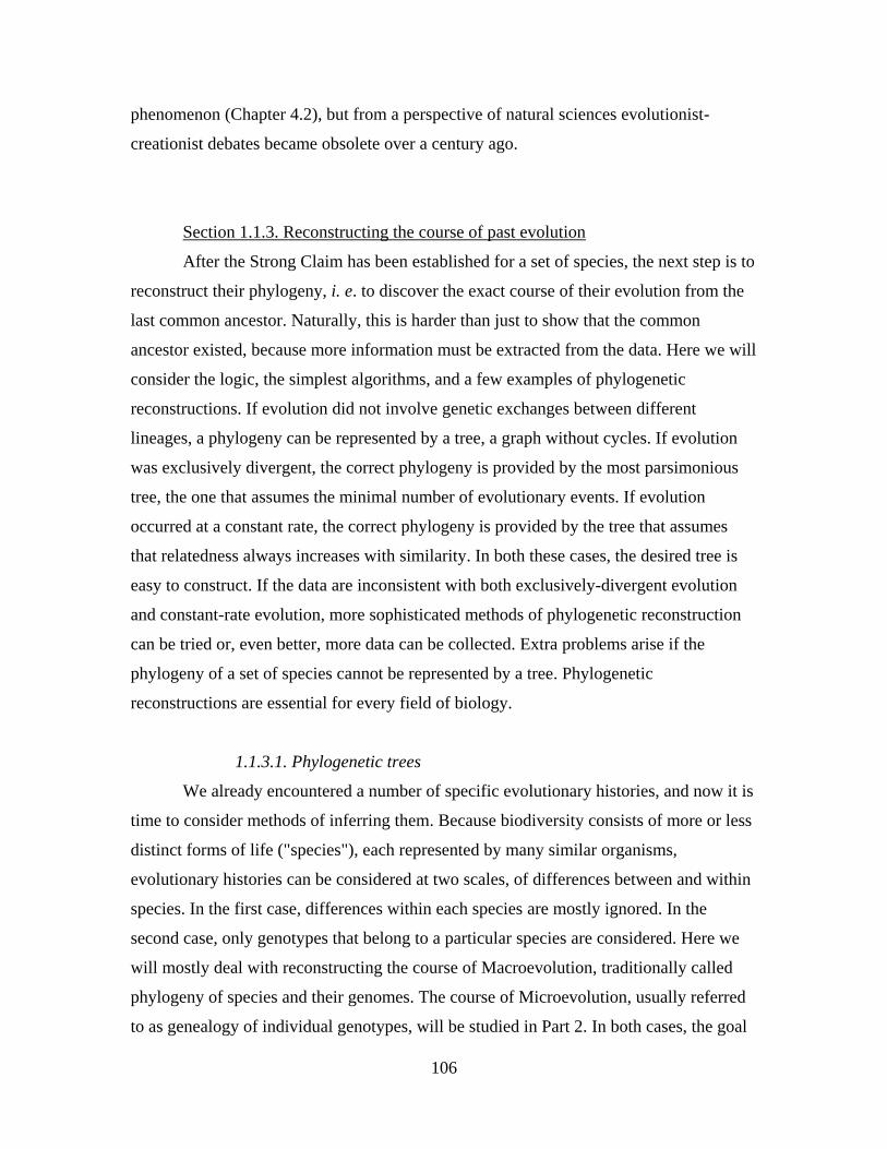
106

phenomenon (Chapter 4.2), but from a perspective of natural sciences evolutionist-

creationist debates became obsolete over a century ago.

Section 1.1.3. Reconstructing the course of past evolution

After the Strong Claim has been established for a set of species, the next step is to

reconstruct their phylogeny, i. e. to discover the exact course of their evolution from the

last common ancestor. Naturally, this is harder than just to show that the common

ancestor existed, because more information must be extracted from the data. Here we will

consider the logic, the simplest algorithms, and a few examples of phylogenetic

reconstructions. If evolution did not involve genetic exchanges between different

lineages, a phylogeny can be represented by a tree, a graph without cycles. If evolution

was exclusively divergent, the correct phylogeny is provided by the most parsimonious

tree, the one that assumes the minimal number of evolutionary events. If evolution

occurred at a constant rate, the correct phylogeny is provided by the tree that assumes

that relatedness always increases with similarity. In both these cases, the desired tree is

easy to construct. If the data are inconsistent with both exclusively-divergent evolution

and constant-rate evolution, more sophisticated methods of phylogenetic reconstruction

can be tried or, even better, more data can be collected. Extra problems arise if the

phylogeny of a set of species cannot be represented by a tree. Phylogenetic

reconstructions are essential for every field of biology.

1.1.3.1. Phylogenetic trees

We already encountered a number of specific evolutionary histories, and now it is

time to consider methods of inferring them. Because biodiversity consists of more or less

distinct forms of life ("species"), each represented by many similar organisms,

evolutionary histories can be considered at two scales, of differences between and within

species. In the first case, differences within each species are mostly ignored. In the

second case, only genotypes that belong to a particular species are considered. Here we

will mostly deal with reconstructing the course of Macroevolution, traditionally called

phylogeny of species and their genomes. The course of Microevolution, usually referred

to as genealogy of individual genotypes, will be studied in Part 2. In both cases, the goal

107

is to reconstruct past evolution of a set of entities under consideration from their last

common ancestor.

A phylogeny (genealogy) can be represented by a tree, a graph without cycles,

only if two conditions are met: (1) we can ignore variation within evolving lineages at

any moment of time and regard each cladogenesis as an instantaneous split and (2)

lineages can diverge but never merge (Fig. 1.1.3.1a). The first condition may complicate

only Macroevolutionary reconstructions. The second issue can complicate reconstructing

the course of both Macroevolution and Microevolution, because genetic exchanges can

involve both distant genomes (due to lateral gene transfer and symbiogenesis) and similar

genotypes (due to sexual reproduction). Still, phylogenetic trees often provide

sufficiently good approximation to reality, and we will start from them.

Fig. 1.1.3.1a. The two conditions necessary for a phylogeny to be representable by a tree.

A phylogenetic tree consists of the root, representing the common ancestor; edges,

representing evolving lineages between successive cladogeneses; internal nodes,

representing common ancestors of subsets of species at the moments of cladogenesis; and

leafs, representing modern species (or genotypes), as well as extinct species that left no

descendants (Fig. 1.1.3.1b). Because a phylogenetic tree represents a process that

occurred in time, each edge has a direction, so that the graph is oriented. When

Macroevolution is considered, phylogenetic trees are conventionally drawn with time

running upward. We will always assume that a tree is binary, i. e. that a lineage can split

only into two lineages at a time. A complete branch of a tree, i. e. an intermediate

ancestor and all its descendants, is called clade. The whole tree is thus a clade originating

from its root. Because we are interested in the course of past evolution that produced a

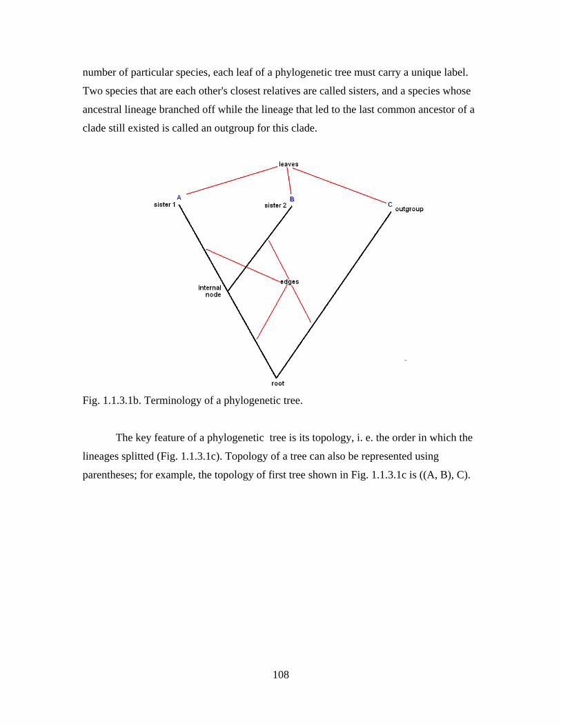
108

number of particular species, each leaf of a phylogenetic tree must carry a unique label.

Two species that are each other's closest relatives are called sisters, and a species whose

ancestral lineage branched off while the lineage that led to the last common ancestor of a

clade still existed is called an outgroup for this clade.

Fig. 1.1.3.1b. Terminology of a phylogenetic tree.

The key feature of a phylogenetic tree is its topology, i. e. the order in which the

lineages splitted (Fig. 1.1.3.1c). Topology of a tree can also be represented using

parentheses; for example, the topology of first tree shown in Fig. 1.1.3.1c is ((A, B), C).

109

Fig. 1.1.3.1c. Topology of a phylogenetic tree. The top four trees all have the same

topology: the first lineage to branch off was that of species C, and this is all that matters

here. The bottom tree has a different topology.

Obviously, there is only a finite number of possible tree topologies for a set of N species.

For N = 1 or 2, there is only one possible topology. A tree with N = 3 can be obtained by

attaching an extra edge to any of the 3 edges of the tree with N = 2, hence there are 3

possible topologies for N = 3 (the first lineage to branch off can be that of A, B, or C).

Analogously, a tree for N = 4 can be obtained by attaching an extra edge to any of the 5

edges of any of the 3 kinds of trees for N = 3; hence, there are 15 possible topologies for

N = 4 (Fig. 1.1.3.1d).

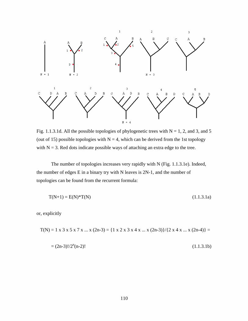
110

Fig. 1.1.3.1d. All the possible topologies of phylogenetic trees with N = 1, 2, and 3, and 5

(out of 15) possible topologies with N = 4, which can be derived from the 1st topology

with N = 3. Red dots indicate possible ways of attaching an extra edge to the tree.

The number of topologies increases very rapidly with N (Fig. 1.1.3.1e). Indeed,

the number of edges E in a binary try with N leaves is 2N-1, and the number of

topologies can be found from the recurrent formula:

T(N+1) = E(N)*T(N) (1.1.3.1a)

or, explicitly

T(N) = 1 x 3 x 5 x 7 x ... x (2n-3) = {1 x 2 x 3 x 4 x ... x (2n-3)}/{2 x 4 x ... x (2n-4)} =

= (2n-3)!/2n(n-2)! (1.1.3.1b)

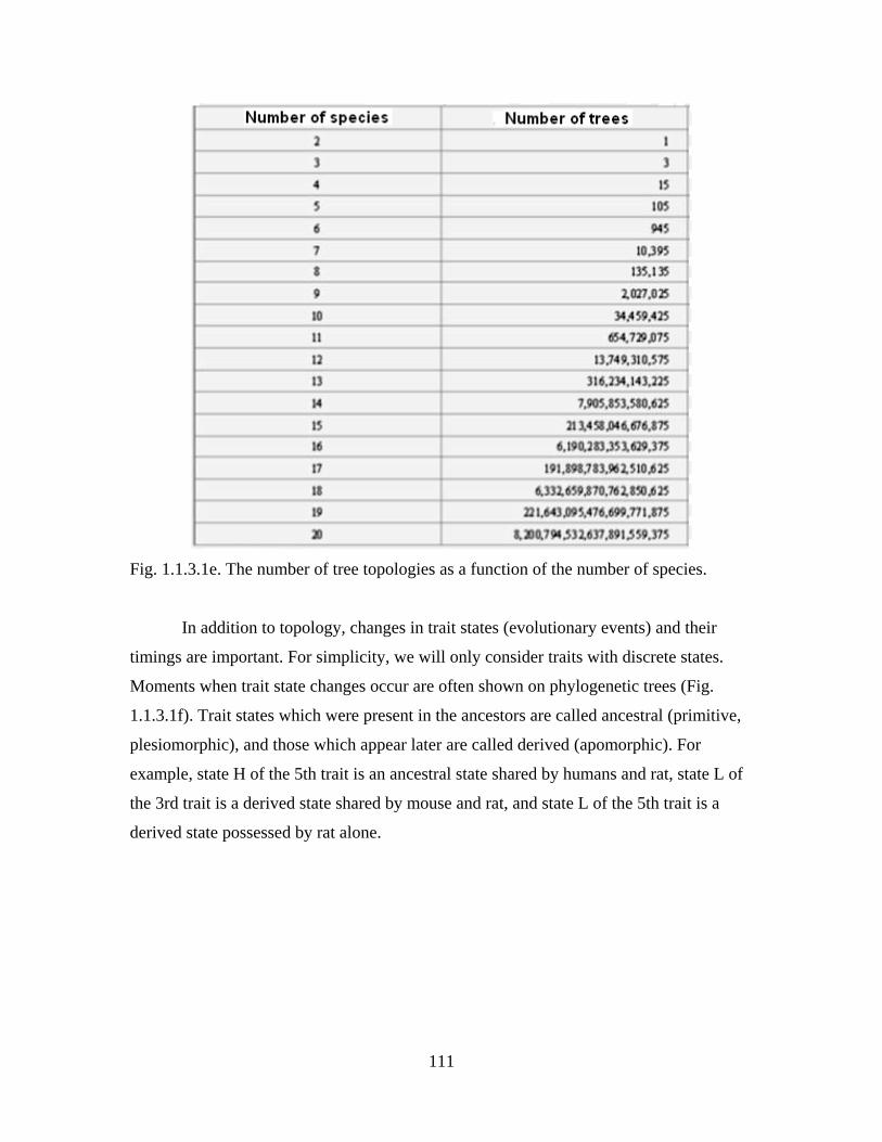
111

Fig. 1.1.3.1e. The number of tree topologies as a function of the number of species.

In addition to topology, changes in trait states (evolutionary events) and their

timings are important. For simplicity, we will only consider traits with discrete states.

Moments when trait state changes occur are often shown on phylogenetic trees (Fig.

1.1.3.1f). Trait states which were present in the ancestors are called ancestral (primitive,

plesiomorphic), and those which appear later are called derived (apomorphic). For

example, state H of the 5th trait is an ancestral state shared by humans and rat, state L of

the 3rd trait is a derived state shared by mouse and rat, and state L of the 5th trait is a

derived state possessed by rat alone.

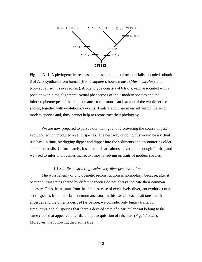
112

Fig. 1.1.3.1f. A phylogenetic tree based on a segment of mitochondrially-encoded subunit

8 of ATP synthase from human (Homo sapiens), house mouse (Mus musculus), and

Norway rat (Rattus norvegicus). A phenotype consists of 6 traits, each associated with a

position within the alignment. Actual phenotypes of the 3 modern species and the

inferred phenotypes of the common ancestor of mouse and rat and of the whole set are

shown, together with evolutionary events. Traits 1 and 6 are invariant within the set of

modern species and, thus, cannot help to reconstruct their phylogeny.

We are now prepared to pursue our main goal of discovering the course of past

evolution which produced a set of species. The best way of doing this would be a virtual

trip back in time, by digging dipper and dipper into the sediments and encountering older

and older fossils. Unfortunately, fossil records are almost never good enough for this, and

we need to infer phylogenies indirectly, mostly relying on traits of modern species.

1.1.3.2. Reconstructing exclusively divergent evolution

The worst enemy of phylogenetic reconstructions is homoplasy, because, after it

occurred, trait states shared by different species do not always indicate their common

ancestry. Thus, let us start from the simplest case of exclusively divergent evolution of a

set of species from their last common ancestor. In this case, in each trait one state is

ancestral and the other is derived (as before, we consider only binary traits, for

simplicity), and all species that share a derived state of a particular trait belong to the

same clade that appeared after the unique acquisition of this state (Fig. 1.1.3.2a).

Moreover, the following theorem is true.

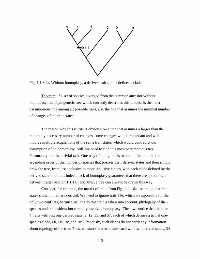
113

Fig. 1.1.3.2a. Without homoplasy, a derived trait state 1 defines a clade.

Theorem: if a set of species diverged from the common ancestor without

homoplasy, the phylogenetic tree which correctly describes this process is the most

parsimonious one among all possible trees, i. e. the one that assumes the minimal number

of changes of the trait states.

The reason why this is true is obvious: on a tree that assumes a larger than the

minimally necessary number of changes, some changes will be redundant and will

involve multiple acquisitions of the same trait states, which would contradict our

assumption of no homoplasy. Still, we need to find this most parsimonious tree.

Fortunately, this is a trivial task. One way of doing this is to sort all the traits in the

ascending order of the number of species that possess their derived states and then simply

draw the tree, from less inclusive to more inclusive clades, with each clade defined by the

derived state of a trait. Indeed, lack of homoplasy guarantees that there are no conflicts

between traits (Section 1.1.1.6) and, thus, a tree can always be drawn this way.

Consider, for example, the matrix of traits from Fig. 1.1.1.6a, assuming that trait

states shown in red are derived. We need to ignore trait 116, which is responsible for the

only two conflicts, because, as long as this trait is taken into account, phylogeny of the 7

species under consideration certainly involved homoplasy. Then, we notice that there are

4 traits with just one derived state, 9, 12, 33, and 57, each of which defines a trivial one-

species clade, Dr, Hs, Rc, and Hr. Obviously, such clades do not carry any information

about topology of the tree. Thus, we start from two traits each with two derived states, 34

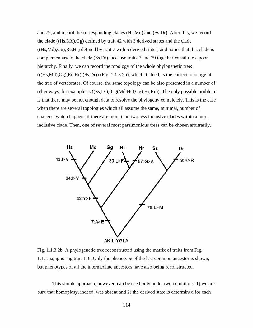
114

and 79, and record the corresponding clades (Hs,Md) and (Ss,Dr). After this, we record

the clade ((Hs,Md),Gg) defined by trait 42 with 3 derived states and the clade

((Hs,Md),Gg),Rc,Hr) defined by trait 7 with 5 derived states, and notice that this clade is

complementary to the clade (Ss,Dr), because traits 7 and 79 together constitute a poor

hierarchy. Finally, we can record the topology of the whole phylogenetic tree:

(((Hs,Md),Gg),Rc,Hr),(Ss,Dr)) (Fig. 1.1.3.2b), which, indeed, is the correct topology of

the tree of vertebrates. Of course, the same topology can be also presented in a number of

other ways, for example as ((Ss,Dr),(Gg(Md,Hs),Gg),Hr,Rc)). The only possible problem

is that there may be not enough data to resolve the phylogeny completely. This is the case

when there are several topologies which all assume the same, minimal, number of

changes, which happens if there are more than two less inclusive clades within a more

inclusive clade. Then, one of several most parsimonious trees can be chosen arbitrarily.

Fig. 1.1.3.2b. A phylogenetic tree reconstructed using the matrix of traits from Fig.

1.1.1.6a, ignoring trait 116. Only the phenotype of the last common ancestor is shown,

but phenotypes of all the intermediate ancestors have also being reconstructed.

This simple approach, however, can be used only under two conditions: 1) we are

sure that homoplasy, indeed, was absent and 2) the derived state is determined for each

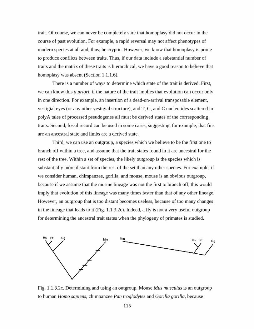
115

trait. Of course, we can never be completely sure that homoplasy did not occur in the

course of past evolution. For example, a rapid reversal may not affect phenotypes of

modern species at all and, thus, be cryptic. However, we know that homoplasy is prone

to produce conflicts between traits. Thus, if our data include a substantial number of

traits and the matrix of these traits is hierarchical, we have a good reason to believe that

homoplasy was absent (Section 1.1.1.6).

There is a number of ways to determine which state of the trait is derived. First,

we can know this a priori, if the nature of the trait implies that evolution can occur only

in one direction. For example, an insertion of a dead-on-arrival transposable element,

vestigial eyes (or any other vestigial structure), and T, G, and C nucleotides scattered in

polyA tales of processed pseudogenes all must be derived states of the corresponding

traits. Second, fossil record can be used in some cases, suggesting, for example, that fins

are an ancestral state and limbs are a derived state.

Third, we can use an outgroup, a species which we believe to be the first one to

branch off within a tree, and assume that the trait states found in it are ancestral for the

rest of the tree. Within a set of species, the likely outgroup is the species which is

substantially more distant from the rest of the set than any other species. For example, if

we consider human, chimpanzee, gorilla, and mouse, mouse is an obvious outgroup,

because if we assume that the murine lineage was not the first to branch off, this would

imply that evolution of this lineage was many times faster than that of any other lineage.

However, an outgroup that is too distant becomes useless, because of too many changes

in the lineage that leads to it (Fig. 1.1.3.2c). Indeed, a fly is not a very useful outgroup

for determining the ancestral trait states when the phylogeny of primates is studied.

Fig. 1.1.3.2c. Determining and using an outgroup. Mouse Mus musculus is an outgroup

to human Homo sapiens, chimpanzee Pan troglodytes and Gorilla gorilla, because

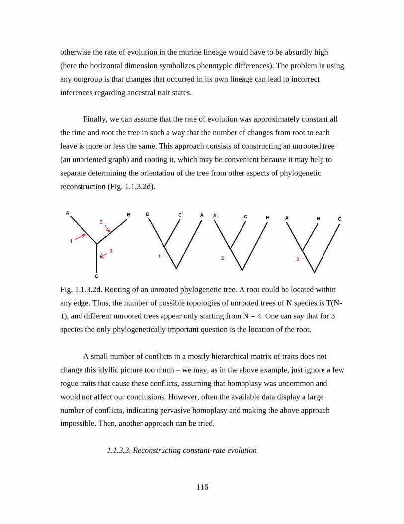
116

otherwise the rate of evolution in the murine lineage would have to be absurdly high

(here the horizontal dimension symbolizes phenotypic differences). The problem in using

any outgroup is that changes that occurred in its own lineage can lead to incorrect

inferences regarding ancestral trait states.

Finally, we can assume that the rate of evolution was approximately constant all

the time and root the tree in such a way that the number of changes from root to each

leave is more or less the same. This approach consists of constructing an unrooted tree

(an unoriented graph) and rooting it, which may be convenient because it may help to

separate determining the orientation of the tree from other aspects of phylogenetic

reconstruction (Fig. 1.1.3.2d).

Fig. 1.1.3.2d. Rooting of an unrooted phylogenetic tree. A root could be located within

any edge. Thus, the number of possible topologies of unrooted trees of N species is T(N-

1), and different unrooted trees appear only starting from N = 4. One can say that for 3

species the only phylogenetically important question is the location of the root.

A small number of conflicts in a mostly hierarchical matrix of traits does not

change this idyllic picture too much – we may, as in the above example, just ignore a few

rogue traits that cause these conflicts, assuming that homoplasy was uncommon and

would not affect our conclusions. However, often the available data display a large

number of conflicts, indicating pervasive homoplasy and making the above approach

impossible. Then, another approach can be tried.

1.1.3.3. Reconstructing constant-rate evolution

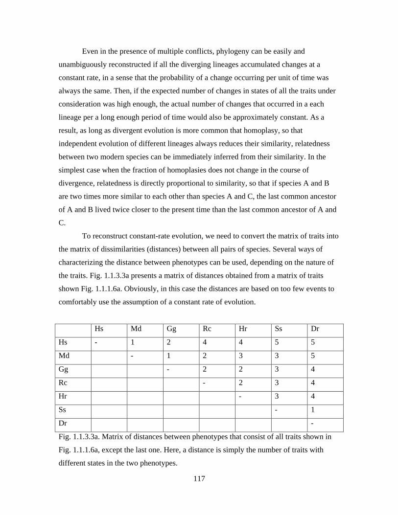
117

Even in the presence of multiple conflicts, phylogeny can be easily and

unambiguously reconstructed if all the diverging lineages accumulated changes at a

constant rate, in a sense that the probability of a change occurring per unit of time was

always the same. Then, if the expected number of changes in states of all the traits under

consideration was high enough, the actual number of changes that occurred in a each

lineage per a long enough period of time would also be approximately constant. As a

result, as long as divergent evolution is more common that homoplasy, so that

independent evolution of different lineages always reduces their similarity, relatedness

between two modern species can be immediately inferred from their similarity. In the

simplest case when the fraction of homoplasies does not change in the course of

divergence, relatedness is directly proportional to similarity, so that if species A and B

are two times more similar to each other than species A and C, the last common ancestor

of A and B lived twice closer to the present time than the last common ancestor of A and

C.

To reconstruct constant-rate evolution, we need to convert the matrix of traits into

the matrix of dissimilarities (distances) between all pairs of species. Several ways of

characterizing the distance between phenotypes can be used, depending on the nature of

the traits. Fig. 1.1.3.3a presents a matrix of distances obtained from a matrix of traits

shown Fig. 1.1.1.6a. Obviously, in this case the distances are based on too few events to

comfortably use the assumption of a constant rate of evolution.

Hs Md Gg Rc Hr Ss Dr

Hs - 1 2 4 4 5 5

Md - 1 2 3 3 5

Gg - 2 2 3 4

Rc - 2 3 4

Hr - 3 4

Ss - 1

Dr -

Fig. 1.1.3.3a. Matrix of distances between phenotypes that consist of all traits shown in

Fig. 1.1.1.6a, except the last one. Here, a distance is simply the number of traits with

different states in the two phenotypes.

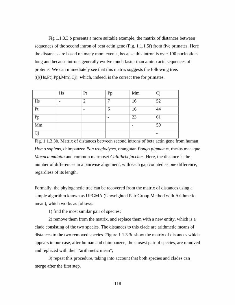
118

Fig 1.1.3.3.b presents a more suitable example, the matrix of distances between

sequences of the second intron of beta actin gene (Fig. 1.1.1.5f) from five primates. Here

the distances are based on many more events, because this intron is over 100 nucleotides

long and because introns generally evolve much faster than amino acid sequences of

proteins. We can immediately see that this matrix suggests the following tree:

((((Hs,Pt),Pp),Mm),Cj), which, indeed, is the correct tree for primates.

Hs Pt Pp Mm Cj

Hs - 2 7 16 52

Pt - 6 16 44

Pp - 23 61

Mm - 50

Cj -

Fig. 1.1.3.3b. Matrix of distances between second introns of beta actin gene from human

Homo sapiens, chimpanzee Pan troglodytes, orangutan Pongo pigmaeus, rhesus macaque

Macaca mulatta and common marmoset Callithrix jacchus. Here, the distance is the

number of differences in a pairwise alignment, with each gap counted as one difference,

regardless of its length.

Formally, the phylogenetic tree can be recovered from the matrix of distances using a

simple algorithm known as UPGMA (Unweighted Pair Group Method with Arithmetic

mean), which works as follows:

1) find the most similar pair of species;

2) remove them from the matrix, and replace them with a new entity, which is a

clade consisting of the two species. The distances to this clade are arithmetic means of

distances to the two removed species. Figure 1.1.3.3c show the matrix of distances which

appears in our case, after human and chimpanzee, the closest pair of species, are removed

and replaced with their "arithmetic mean";

3) repeat this procedure, taking into account that both species and clades can

merge after the first step.

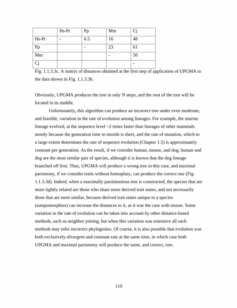
119

Hs-Pt Pp Mm Cj

Hs-Pt - 6.5 16 48

Pp - 23 61

Mm - 50

Cj -

Fig. 1.1.3.3c. A matrix of distances obtained at the first step of application of UPGMA to

the data shown in Fig. 1.1.3.3b.

Obviously, UPGMA produces the tree in only N steps, and the root of the tree will be

located in its middle.

Unfortunately, this algorithm can produce an incorrect tree under even moderate,

and feasible, variation in the rate of evolution among lineages. For example, the murine

lineage evolved, at the sequence level ~2 times faster than lineages of other mammals

mostly because the generation time in murids is short, and the rate of mutation, which to

a large extent determines the rate of sequence evolution (Chapter 1.5) is approximately

constant per generation. As the result, if we consider human, mouse, and dog, human and

dog are the most similar pair of species, although it is known that the dog lineage

branched off first. Thus, UPGMA will produce a wrong tree in this case, and maximal

parsimony, if we consider traits without homoplasy, can produce the correct one (Fig.

1.1.3.3d). Indeed, when a maximally parsimonious tree is constructed, the species that are

more tightly related are those who share more derived trait states, and not necessarily

those that are most similar, because derived trait states unique to a species

(autapomorphies) can increase the distances to it, as it was the case with mouse. Some

variation in the rate of evolution can be taken into account by other distance-based

methods, such as neighbor joining, but when this variation was extensive all such

methods may infer incorrect phylogenies. Of course, it is also possible that evolution was

both exclusively-divergent and constant-rate at the same time, in which case both

UPGMA and maximal parsimony will produce the same, and correct, tree.

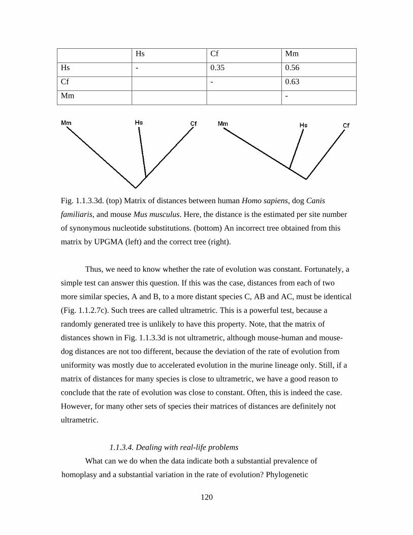
120

Hs Cf Mm

Hs - 0.35 0.56

Cf - 0.63

Mm -

Fig. 1.1.3.3d. (top) Matrix of distances between human Homo sapiens, dog Canis

familiaris, and mouse Mus musculus. Here, the distance is the estimated per site number

of synonymous nucleotide substitutions. (bottom) An incorrect tree obtained from this

matrix by UPGMA (left) and the correct tree (right).

Thus, we need to know whether the rate of evolution was constant. Fortunately, a

simple test can answer this question. If this was the case, distances from each of two

more similar species, A and B, to a more distant species C, AB and AC, must be identical

(Fig. 1.1.2.7c). Such trees are called ultrametric. This is a powerful test, because a

randomly generated tree is unlikely to have this property. Note, that the matrix of

distances shown in Fig. 1.1.3.3d is not ultrametric, although mouse-human and mouse-

dog distances are not too different, because the deviation of the rate of evolution from

uniformity was mostly due to accelerated evolution in the murine lineage only. Still, if a

matrix of distances for many species is close to ultrametric, we have a good reason to

conclude that the rate of evolution was close to constant. Often, this is indeed the case.

However, for many other sets of species their matrices of distances are definitely not

ultrametric.

1.1.3.4. Dealing with real-life problems

What can we do when the data indicate both a substantial prevalence of

homoplasy and a substantial variation in the rate of evolution? Phylogenetic

121

reconstructions in such situations, which are quite common, is a huge and a rather

technically difficult subject. Still, basically there are just two options – to try to extract

phylogenetic information from less-than-perfect data and to obtain better data.

When the matrix of traits contains a lot of conflicts, finding the maximally

parsimonious tree becomes what is known in computer science as an NP-hard problem:

the only way of solving it with certainty is to evaluate all possible trees, which is

impossible for N > 10-20 (Fig. 1.1.3.1e). Even worse, with substantial homoplasy, the

maximally parsimonious tree may not reflect what had actually happened. In particular, it

may be more parsimonious to assume that lineages which independently accumulated a

lot of changes, some of which homoplasious, form clades (long-branch attraction),

because the correct phylogeny may involve more homoplasy than what is revealed by

conflicts within the data.

With imperfect data, phylogenetic inference becomes a probabilistic problem,

because we cannot be absolutely sure that any tree we construct reflects the course of

past evolution. Thus, we can only try to find one or several trees that are the most

"probable", given the data. A widely used statistical approach to such problems, not

confined to problems of biological origin, is called maximal likelihood (ML).

Very basically, ML works as follows. We have some observable data D (the

matrix of traits for N species, in the case of phylogenetic reconstructions), and a number

of possible unobservable hypotheses H (all possible T(N) trees for N species). Suppose

that for each hypothesis we can calculate P(D|H), the conditional probability that, if this

hypothesis was correct, it produces the data that we actually observe. In our case, P(D|H)

is the probability that evolution of a set of species from their common ancestor that

followed the course described by a particular tree H will lead to the observed matrix of

traits D. Then, we interpret P(D|H) as the likelihood of the tree H given the matrix of

traits D. The word likelihood is used, because P(D|H) is not the probability of a

hypothesis given the data, since the sum of P(D|H) for a particular D and all possible H is

not necessarily 1. Finally, we say that the tree that, for the observed matrix of traits,

produces the highest P(D|H) is the most likely one, and try to find it.

Finding the ML tree may be technically difficult, but there are many algorithms

and software tools that can be used with a good deal of success. A fundamental issue,

however, is that determining P(D|H) requires some a priori knowledge on how evolution

122

proceeded. For example, the probability of observing a particular matrix of traits after

evolution that followed the course described by a particular tree depends on whether

different kinds of changes in trait states (for example, transitions and transversion) were

equally probable or not. Such information must be obtained somehow and supplied to an

algorithm that calculates the ML tree. Of course, this can reduce our confidence in the

results, because we may not know exactly how evolution occurred.

An even more ambitious approach is to explicitly evaluate P(H|D), the conditional

probability that a tree is correct given that a particular matrix of traits has been observed.

This can be done using the basic fact on conditional probability, known as Bayes

formula:

P(H|D) = (P(D|H)xP(H))/P(D) (1.1.3.4)

where P(H), the probability of a hypothesis, is an a priori (prior) probability of the tree

(before we consider any data) and P(D), the probability of the data, is simply the sum of

numerators for all possible trees (thus, P(H|D) is, indeed, a probability). Here, in addition

to problems associated with evaluating P(D|H), we also need to somehow determine the

prior distribution P(H). However, we make have no a priori idea on which trees are more

probable. Still, Bayesian methods are widely used, under a variety of assumptions, due to

their computational convenience.

Obviously, neither of these two approaches is perfect. The same is true for a

variety of other approaches developed for inferring phylogenies from noisy data. Thus,

collecting better data may be a way to go in tough cases.

We cannot do much about unequal rates of evolution in different lineages, but we

can look for traits that are less prone to homoplasy. This idea goes back to Darwin, who

suggested, in modern terms, that traits involved in adaptation to specific conditions are

less suitable for phylogenetic reconstructions. It is also obvious that simple traits with a

small number of possible states, such as a nucleotide or an amino acid that occupies a

particular position within the sequence alignment, are inherently prone to homoplasy, so

that using complex traits, such as microinversions, is better, although this requires more

sequence data.

123

The choice of suitable traits depends on how similar to each other are the species

from the set whose phylogeny we are trying to infer, because useful phylogenetic traits

must evolve neither too slow nor too fast. Indeed, a trait that evolved too fast within the

set of species will remain invariant and be useless, and a trait that evolved too fast will

accumulate a lot of homoplasies, also making it useless. Fortunately, there are good traits

for all kinds of phylogenetic reconstructions.

For very similar species, such as different apes, positions within alignments of

rapidly-evolving segments of non-coding are suitable (Fig. 1.1.3.3b). For moderately

similar species, such as different primates, complex traits associated with non-coding

DNA, such microinversions and TE insertions, may be the best (Fig. 1.1.2.5a). For still

less similar species, like all mammals and even all vertebrates, similarity between non-

coding DNA sequences is mostly lost, but we may use traits associated with gene order

(Fig. 1.1.2.4f). Finally, when we consider really dissimilar species, all sequence-level

similarities between them are lost, except those between amino acid sequences of some

proteins, so that we need again to consider alignments but now concentrate on the most

conservative sites in the most conservative proteins. Fortunately, there are not too many

deep branches on the tree of life that require using such traits, and they have already been

resolved. Modern organisms contain enough information to resolve their phylogenies,

and the universal tree of life is now not that far from being resolved.

1.1.3.5. Phylogenies which are not trees

A phylogeny not always can be represented by a tree (Fig. 1.1.3.1a). First,

variation within individual lineages may be impossible to ignore, which is the case when

highly variable sexual species undergo cladogeneses in a rapid succession. In this case,

"lineage sorting" can lead to different parts of the genome having different phylogenies

(Fig. 1.1.3.5a). This certainly must be taken onto account sometimes, but is not crucial

when distant enough species are considered.

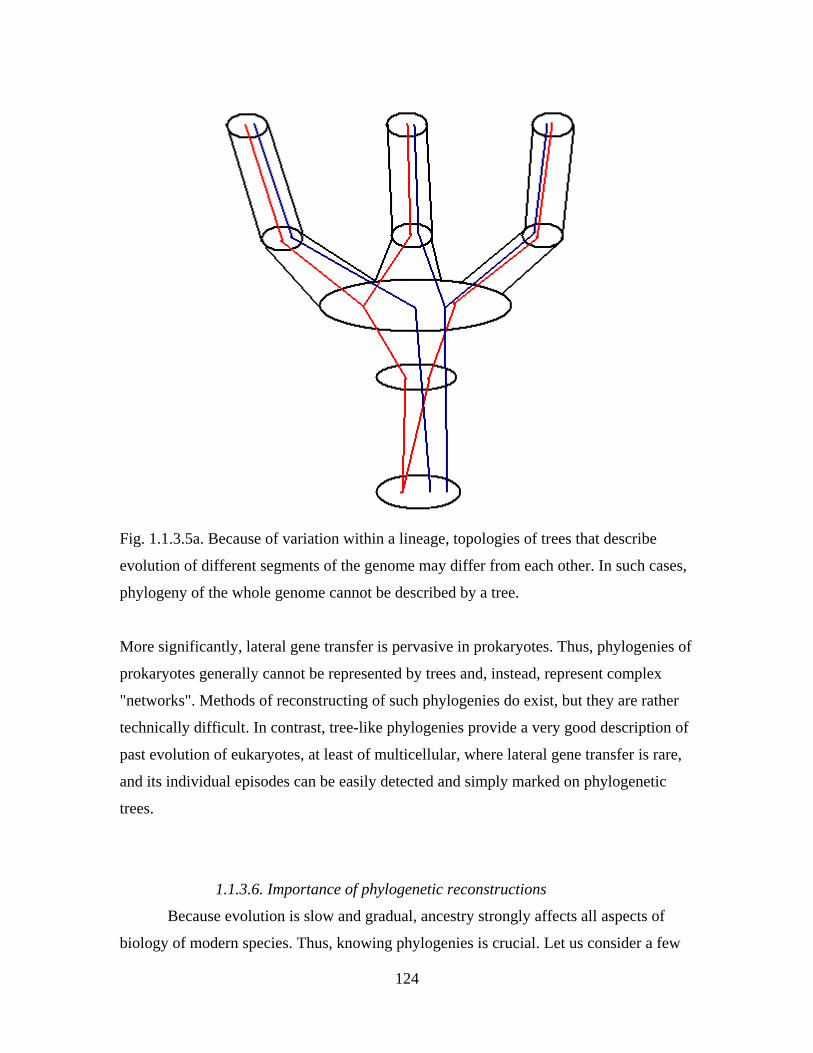
124

Fig. 1.1.3.5a. Because of variation within a lineage, topologies of trees that describe

evolution of different segments of the genome may differ from each other. In such cases,

phylogeny of the whole genome cannot be described by a tree.

More significantly, lateral gene transfer is pervasive in prokaryotes. Thus, phylogenies of

prokaryotes generally cannot be represented by trees and, instead, represent complex

"networks". Methods of reconstructing of such phylogenies do exist, but they are rather

technically difficult. In contrast, tree-like phylogenies provide a very good description of

past evolution of eukaryotes, at least of multicellular, where lateral gene transfer is rare,

and its individual episodes can be easily detected and simply marked on phylogenetic

trees.

1.1.3.6. Importance of phylogenetic reconstructions

Because evolution is slow and gradual, ancestry strongly affects all aspects of

biology of modern species. Thus, knowing phylogenies is crucial. Let us consider a few

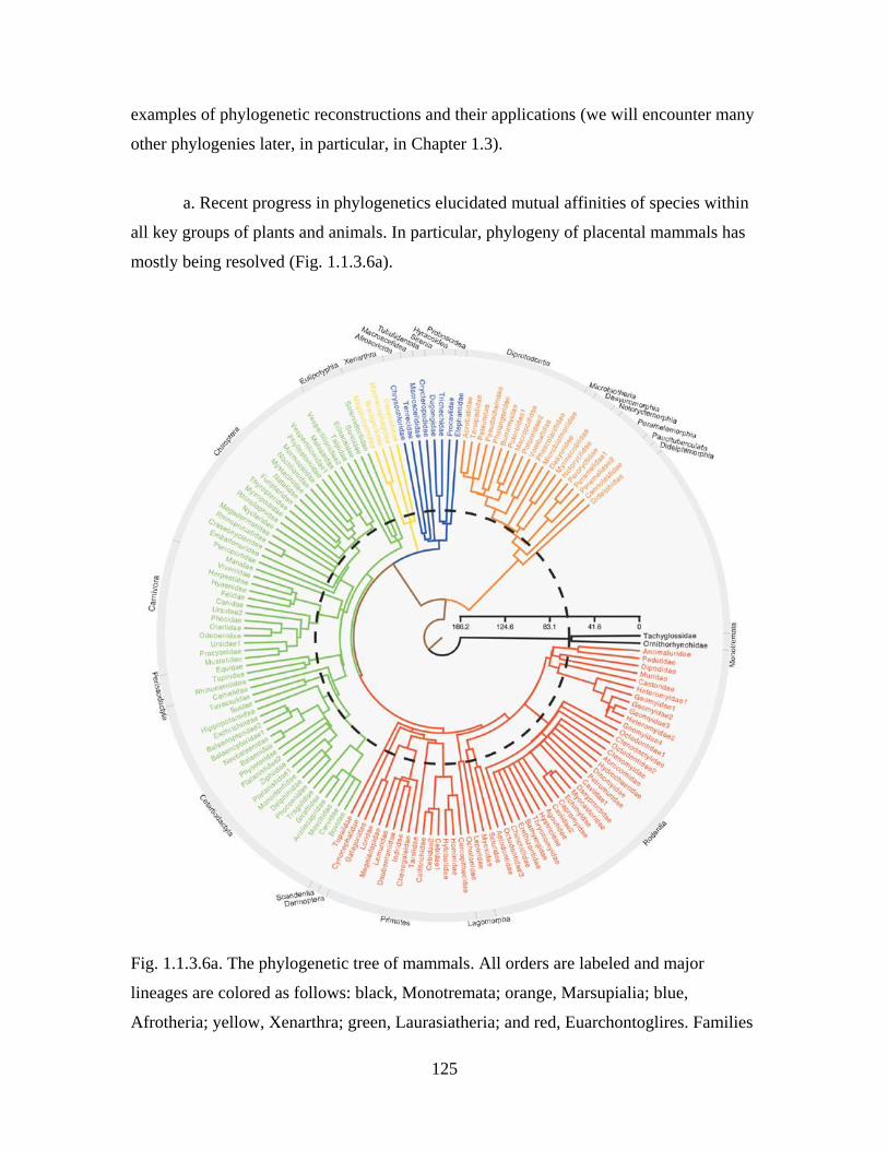
125

examples of phylogenetic reconstructions and their applications (we will encounter many

other phylogenies later, in particular, in Chapter 1.3).

a. Recent progress in phylogenetics elucidated mutual affinities of species within

all key groups of plants and animals. In particular, phylogeny of placental mammals has

mostly being resolved (Fig. 1.1.3.6a).

Fig. 1.1.3.6a. The phylogenetic tree of mammals. All orders are labeled and major

lineages are colored as follows: black, Monotremata; orange, Marsupialia; blue,

Afrotheria; yellow, Xenarthra; green, Laurasiatheria; and red, Euarchontoglires. Families

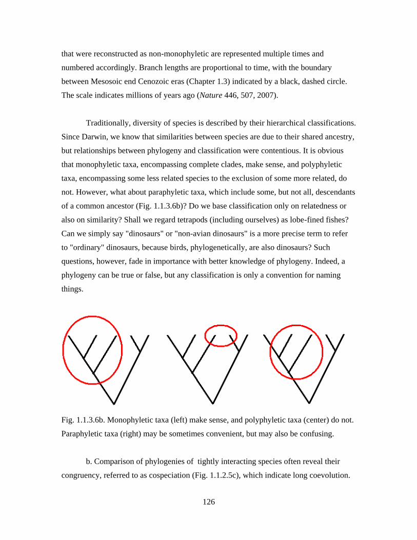
126

that were reconstructed as non-monophyletic are represented multiple times and

numbered accordingly. Branch lengths are proportional to time, with the boundary

between Mesosoic end Cenozoic eras (Chapter 1.3) indicated by a black, dashed circle.

The scale indicates millions of years ago (Nature 446, 507, 2007).

Traditionally, diversity of species is described by their hierarchical classifications.

Since Darwin, we know that similarities between species are due to their shared ancestry,

but relationships between phylogeny and classification were contentious. It is obvious

that monophyletic taxa, encompassing complete clades, make sense, and polyphyletic

taxa, encompassing some less related species to the exclusion of some more related, do

not. However, what about paraphyletic taxa, which include some, but not all, descendants

of a common ancestor (Fig. 1.1.3.6b)? Do we base classification only on relatedness or

also on similarity? Shall we regard tetrapods (including ourselves) as lobe-fined fishes?

Can we simply say "dinosaurs" or "non-avian dinosaurs" is a more precise term to refer

to "ordinary" dinosaurs, because birds, phylogenetically, are also dinosaurs? Such

questions, however, fade in importance with better knowledge of phylogeny. Indeed, a

phylogeny can be true or false, but any classification is only a convention for naming

things.

Fig. 1.1.3.6b. Monophyletic taxa (left) make sense, and polyphyletic taxa (center) do not.

Paraphyletic taxa (right) may be sometimes convenient, but may also be confusing.

b. Comparison of phylogenies of tightly interacting species often reveal their

congruency, referred to as cospeciation (Fig. 1.1.2.5c), which indicate long coevolution.

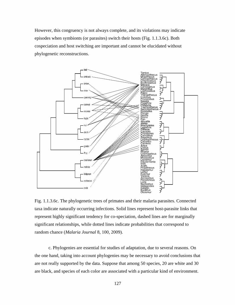
127

However, this congruency is not always complete, and its violations may indicate

episodes when symbionts (or parasites) switch their hosts (Fig. 1.1.3.6c). Both

cospeciation and host switching are important and cannot be elucidated without

phylogenetic reconstructions.

Fig. 1.1.3.6c. The phylogenetic trees of primates and their malaria parasites. Connected

taxa indicate naturally occurring infections. Solid lines represent host-parasite links that

represent highly significant tendency for co-speciation, dashed lines are for marginally

significant relationships, while dotted lines indicate probabilities that correspond to

random chance (Malaria Journal 8, 100, 2009).

c. Phylogenies are essential for studies of adaptation, due to several reasons. On

the one hand, taking into account phylogenies may be necessary to avoid conclusions that

are not really supported by the data. Suppose that among 50 species, 20 are white and 30

are black, and species of each color are associated with a particular kind of environment.

128

If each species represented an independent data point, this would be a significant

association, suggesting an adaptive importance of color. However, a phylogeny may

reveal that there was only one change of color in the course of evolution, making

statistical conclusions impossible.

One the other hand, mapping states of different traits on the same phylogeny often

make it possible to arrive to important conclusions. For example, eusociality in

hymenopterans evolved many times independently, and every time it occurred within a

lineage with monogamous females (Fig. 1.1.3.6d). This pattern supports the hypothesis

that eusociality evolved due to kin selection (Part 3).

129

Fig. 1.1.3.6d. Phylogeny of eusocial Hymenoptera (ants, bees, and wasps). Each

independent origin of eusociality is indicated by alternately colored clades. Clades

130

exhibiting high polyandry (>2 effective mates) have solid red branches, those exhibiting

facultative low polyandry (>1 but <2 effective mates) have dotted red branches, and

entirely monogamous genera have solid black branches (Science 320, 1213, 2008).

Still, it is important to avoid simplistic phylogeny-based conclusions about

adaptation. In particular, there is no firm relationship between branching order and

primitivity. Species that belong to the earliest branches within a clade, such as Amborella

and Nymphales within flowering plants (Chapter 1.3) do not necessarily possess less

derived trait states that other species. Moreover, primitive trait states are not necessarily

"bad" in any sense, e. g., vestigial eye of cave animals are derived states. Finally, we

cannot talk about more and less ancient species, because all modern species originated

from LUCA, so that the expression "living fossils" simply refers to species that evolved

slowly, at least in those traits that are preserved in fossils (Chapter 1.2).

d. Phylogenies are also necessary for studying biogeography. Current

geographical distributions of species are the product of past geological events, vicariant

evolution that followed the origin of geographical barriers (Subsection 1.1.2.7), and

dispersal across such barriers. A substantial correspondence between a phylogeny and the

history of area splits indicates a large role of vicariance in cladogeneses within a

particular group (Fig. 1.1.3.6e). In some groups, however, their current diversity was

mostly shaped by long-distance dispersal (Fig. 1.1.3.6f).

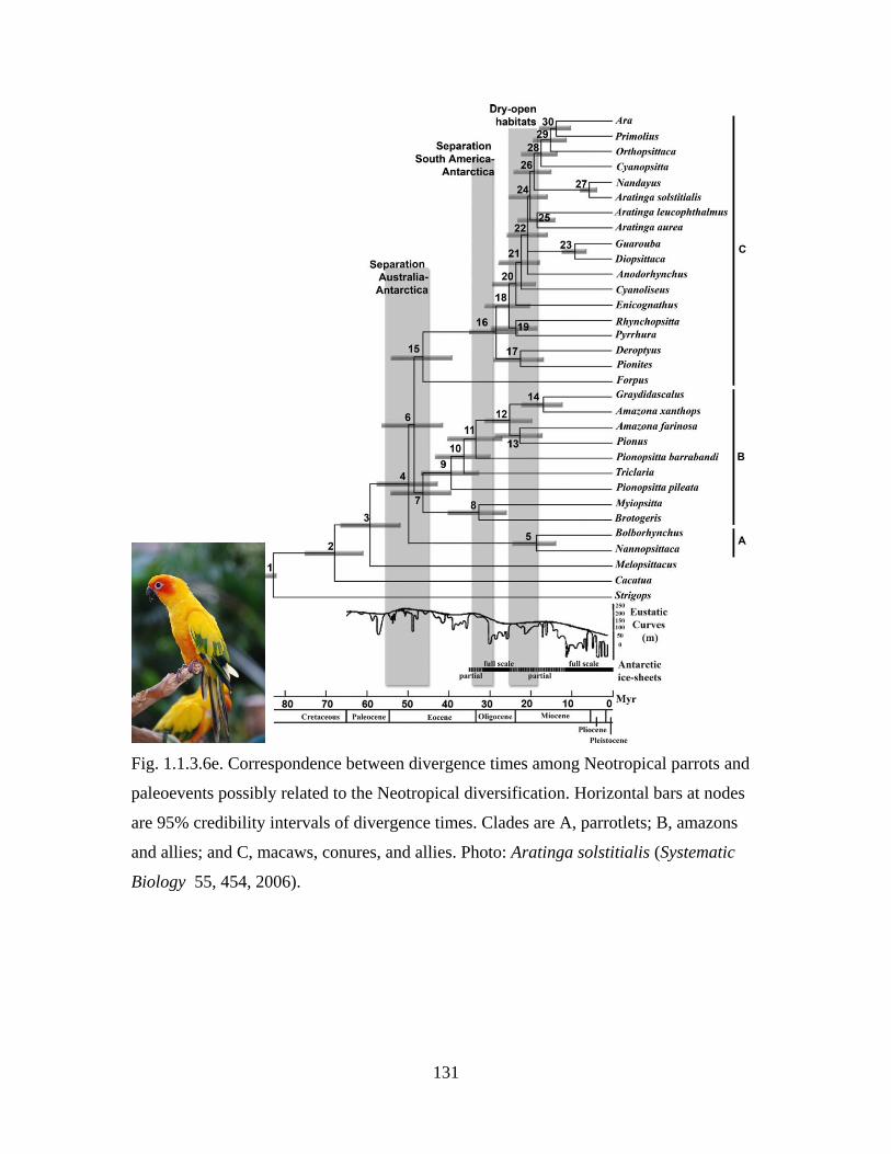
131

Fig. 1.1.3.6e. Correspondence between divergence times among Neotropical parrots and

paleoevents possibly related to the Neotropical diversification. Horizontal bars at nodes

are 95% credibility intervals of divergence times. Clades are A, parrotlets; B, amazons

and allies; and C, macaws, conures, and allies. Photo: Aratinga solstitialis (Systematic

Biology 55, 454, 2006).

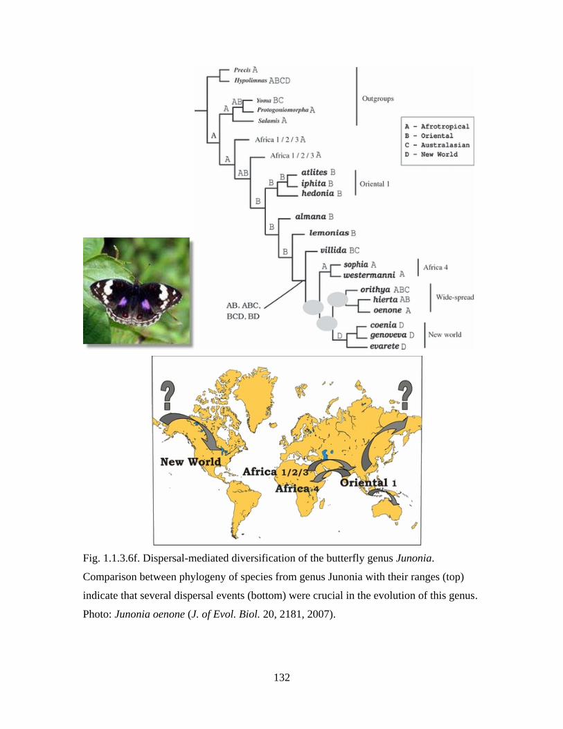
132

Fig. 1.1.3.6f. Dispersal-mediated diversification of the butterfly genus Junonia.

Comparison between phylogeny of species from genus Junonia with their ranges (top)

indicate that several dispersal events (bottom) were crucial in the evolution of this genus.

Photo: Junonia oenone (J. of Evol. Biol. 20, 2181, 2007).

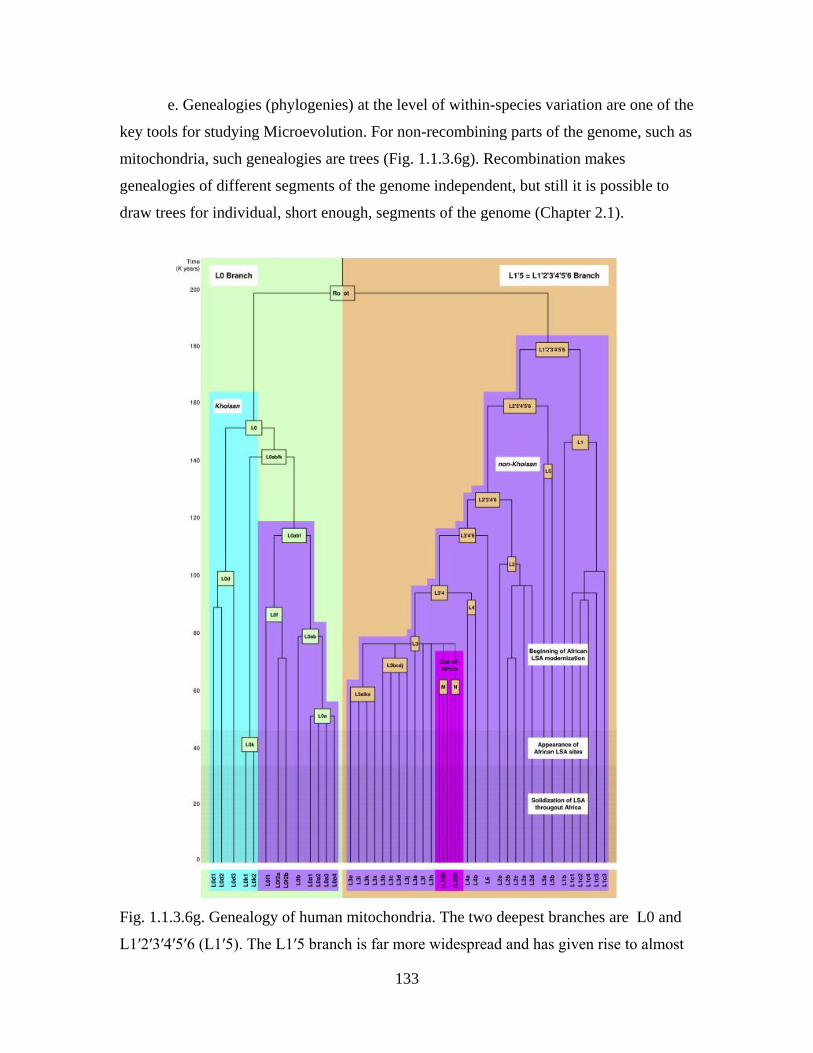
133

e. Genealogies (phylogenies) at the level of within-species variation are one of the

key tools for studying Microevolution. For non-recombining parts of the genome, such as

mitochondria, such genealogies are trees (Fig. 1.1.3.6g). Recombination makes

genealogies of different segments of the genome independent, but still it is possible to

draw trees for individual, short enough, segments of the genome (Chapter 2.1).

Fig. 1.1.3.6g. Genealogy of human mitochondria. The two deepest branches are L0 and

L1′2′3′4′5′6 (L1′5). The L1′5 branch is far more widespread and has given rise to almost

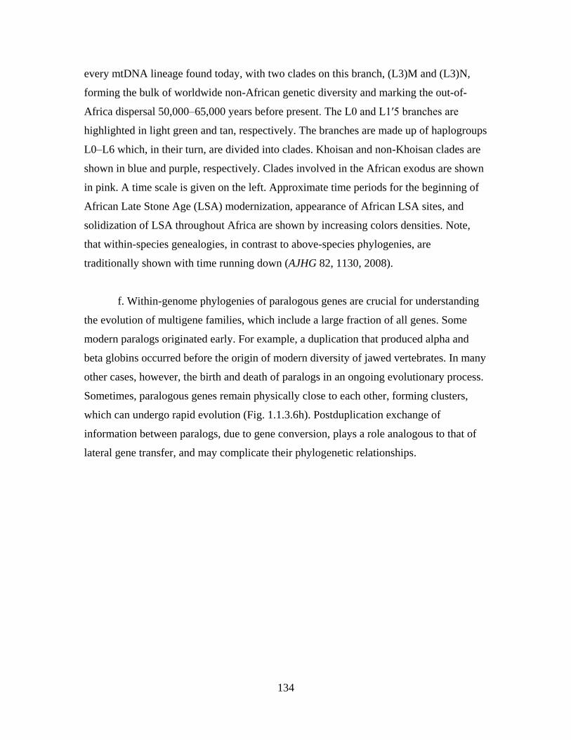
134

every mtDNA lineage found today, with two clades on this branch, (L3)M and (L3)N,

forming the bulk of worldwide non-African genetic diversity and marking the out-of-

Africa dispersal 50,000–65,000 years before present. The L0 and L1′5 branches are

highlighted in light green and tan, respectively. The branches are made up of haplogroups

L0–L6 which, in their turn, are divided into clades. Khoisan and non-Khoisan clades are

shown in blue and purple, respectively. Clades involved in the African exodus are shown

in pink. A time scale is given on the left. Approximate time periods for the beginning of

African Late Stone Age (LSA) modernization, appearance of African LSA sites, and

solidization of LSA throughout Africa are shown by increasing colors densities. Note,

that within-species genealogies, in contrast to above-species phylogenies, are

traditionally shown with time running down (AJHG 82, 1130, 2008).

f. Within-genome phylogenies of paralogous genes are crucial for understanding

the evolution of multigene families, which include a large fraction of all genes. Some

modern paralogs originated early. For example, a duplication that produced alpha and

beta globins occurred before the origin of modern diversity of jawed vertebrates. In many

other cases, however, the birth and death of paralogs in an ongoing evolutionary process.

Sometimes, paralogous genes remain physically close to each other, forming clusters,

which can undergo rapid evolution (Fig. 1.1.3.6h). Postduplication exchange of

information between paralogs, due to gene conversion, plays a role analogous to that of

lateral gene transfer, and may complicate their phylogenetic relationships.

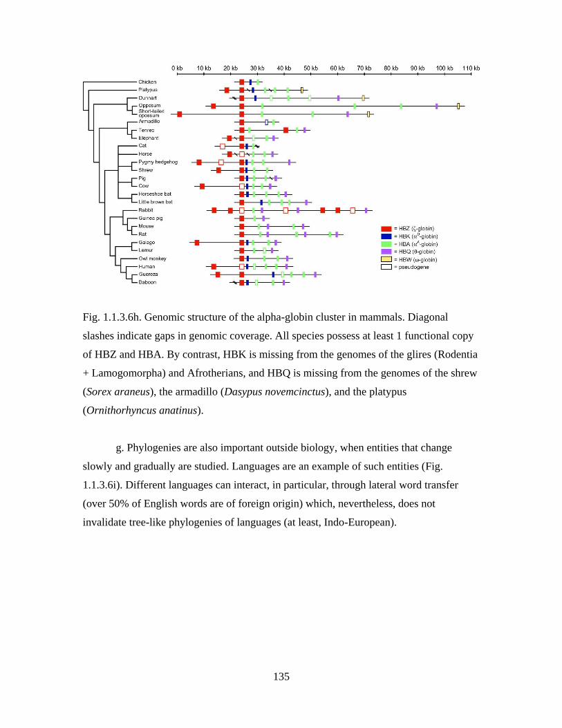
135

Fig. 1.1.3.6h. Genomic structure of the alpha-globin cluster in mammals. Diagonal

slashes indicate gaps in genomic coverage. All species possess at least 1 functional copy

of HBZ and HBA. By contrast, HBK is missing from the genomes of the glires (Rodentia

+ Lamogomorpha) and Afrotherians, and HBQ is missing from the genomes of the shrew

(Sorex araneus), the armadillo (Dasypus novemcinctus), and the platypus

(Ornithorhyncus anatinus).

g. Phylogenies are also important outside biology, when entities that change

slowly and gradually are studied. Languages are an example of such entities (Fig.

1.1.3.6i). Different languages can interact, in particular, through lateral word transfer

(over 50% of English words are of foreign origin) which, nevertheless, does not

invalidate tree-like phylogenies of languages (at least, Indo-European).

136

Fig. 1.1.3.6i. Phylogeny of Indo-European languages. Numbers indicate inferred times of

divergence (Nature 426, 435, 2003).

However, not all things are like evolving species or languages. For example,

transmutations of atoms are not evolutionary but revolutionary – a radioactive decay of

137

an alkali metal K40 creates, in one step, a noble gas Ar40. Atoms have no memory: we

do not care about the ancestry of a particular Ar40 atom – there may be many, all

creating exactly the same entity (perfect homoplasy). As a result, Mendeleev's periodic

table of chemical elements is not phylogenetic.

History and perspectives

Many insights relevant to the evolution of life were made before Darwin. Quintus

Ennius and, no doubt, many people before him, noticed a striking similarity between

humans and monkeys. Carl Linneus realized that hierarchical distributions of traits are

pervasive among modern species of multicellular eukaryotes and used this pattern to

develop his hierarchical classification. Richard Owen introduced the notion of homology.

Joffrua St. Hillarie considered vestigial structures. Finally, Jean Baptiste Lamarck

proposed the first coherent concept of evolution, and Alfred Russel Wallace discovered

evolution by natural selection independently of Darwin. Still, these developments are

currently of interest only to historians of science (e. g., Mayr, 1982).

Modern era in evolutionary biology, and in biology as a whole, begun 136 years

ago in 1859, with the publication of "The Origin of Species by Means of Natural

Selection, or the Preservation of Favored Varieties in the Struggle for Existence" (known

simply as the "Origin of Species") by Charles Robert Darwin. Since then, Darwinian

thinking remains at the foundation of evolutionary biology. Reading Origin of Species

can still be highly recommended, despite the astonishing progress of biology since its

publication. To understand this book, it is essential to recognize its two opposite and

complementary themes. On the one hand, Darwin introduced indirect evidence for

evolution, provided by patterns that cannot be explained by adaptation to current

environments. On the other hand, Darwin discovered natural selection as the key force

responsible for evolution, which strives to adapt species to their current environments. Of

course, there is no contradiction between these two themes: natural selection is not

omnipotent, because it can induce only slow, gradual changes and has no foresight.

Treatment of indirect evidence for past evolution in this Chapter is fully within

the Darwin's paradigm, although I disagree with him on several minor issues, such as

whether environment-specific adaptations, within-species phenotype-level homologies,

or suboptimality of ranges of individual species constitute evidence for evolution. Also,

138

most of scenario-based, and all theory-based, evidence became known only relatively

recently. Finally, Darwin often compared evolutionary explanations of data with

explanations that assume supernatural creation of modern life. Currently, this is out of

fashion – scientists no longer feel qualified to speculate about supernatural.

Being a genius, Darwin had a direct access to mysteries of nature and often did

not explain his reasoning in any detail. For example, introducing hierarchical

distributions of traits as indirect evidence for past evolution – perhaps the most

conceptually difficult kind of such evidence – he basically said only the following:

"From the first dawn of life, all organic beings are found to resemble each other in

descending degrees, so that they can be classed in groups under groups. ... Naturalists try

to arrange the species, genera, and families in each class, on what is called the Natural

System. But what is meant by this system? Some authors look at it merely as a scheme

for arranging together those living objects which are most alike, and for separating those

which are most unlike ... I believe that something more is included; and that propinquity

of descent, the only known cause of the similarity of organic beings, is the bond, hidden

as it is by various degrees of modification, which is partially revealed to us by our

classifications." (Chapter 13).

after which he goes on to offer a rule for recognizing traits that are, in modern terms, less

prone to homoplasy and, thus, are more suitable for phylogenetic reconstructions ("It may

even be given as a general rule, that the less any part of the organization is concerned

with special habits, the more important it becomes for classification."). Here, I tried to

make explicit all the steps in the Darwinian analysis, in this and other cases.

Soon after 1859, past evolution of life became universally accepted by biologists.

New indirect evidence for it kept accumulating slowly, until the genomic revolution,

which provided the whole new realm of evidence based on DNA sequences, that contain

a lot of information and are relatively simple, in comparison to higher-level phenotypes.

Also, old-fashioned paleontological discoveries provided, and keep providing, new

spectacular direct evidence of past evolution (Chapter 1.2 and 1.3).

Common ancestry of all modern life implies that its phylogeny must be studied.

For a long time after Darwin, however, the progress in inferring phylogenies was very

139

slow, and there were no universally accepted solutions to even the most fundamental

phylogenetic issues such that mutual affinities of large groups ("Kingdoms") of life or the

ancestry of land plants. Phylogenetics begun to advance only in the second half of the

XX century, due to development of algorithms, availability of computers, and the flood

of sequence data. Indeed, a sequence contains much more traits that could ever by

recognized morphologically, and one does not need to be a specialist to study phylogeny

of a particular group of species. This led to a spectacular progress, and now most of

large-scale phylogenetic issues have already been resolved. It is worth noting that the key

role in the development maximal likelihood, a general statistical method widely used in

modern phylogenetics, was played by Ronald Aylmer Fisher, a scientist who also laid the

foundations of genetical studies of Microevolution (Part 2).

Perspectives. Better understanding of functioning of complex phenotypes will

lead to more information on fitness landscapes and, thus, on suboptimality and

homology. In not-too-distant future we can expect to see direct demonstrations that a

particular function, at least at the molecular level, can be performed in very many

different ways. This will lead to better understanding of evolution in general, and of

indirect evidence for past evolution, in particular. Continuous rapid progress of

phylogenetics will lead to more and more detailed knowledge of the universal tree of life,

although studying all species in groups like insects will take a while. Data on complete

sequences of genomes of multiple species will provide more suitable traits for

phylogenetic reconstructions in difficult cases and will probably reduce the importance of

sophisticated computational methods.