American Mathematical Society

Pascal CherrierAlbert Milani

Linear and Quasi-linear Evolution Equationsin Hilbert Spaces

Graduate Studies in Mathematics

Volume 135

Linear and Quasi-linear Evolution Equations in Hilbert Spaces

Linear and Quasi-linear Evolution Equations in Hilbert Spaces

Pascal Cherrier Albert Milani

American Mathematical SocietyProvidence, Rhode Island

Graduate Studies in Mathematics

Volume 135

http://dx.doi.org/10.1090/gsm/135

EDITORIAL COMMITTEE

David Cox (Chair)Daniel S. FreedRafe Mazzeo

Gigliola Staffilani

2010 Mathematics Subject Classification. Primary 35L15,35L72, 35K15, 35K59, 35Q61, 35Q74.

For additional information and updates on this book, visitwww.ams.org/bookpages/gsm-135

Library of Congress Cataloging-in-Publication Data

Cherrier, Pascal, 1950–Linear and quasi-linear evolution equations in Hilbert spaces / Pascal Cherrier, Albert Milani.

p. cm. — (Graduate studies in mathematics ; v. 135)Includes bibliographical references and index.ISBN 978-0-8218-7576-6 (alk. paper)1. Initial value problems. 2. Differential equations, Hyperbolic. 3. Evolution equations.

4. Hilbert space. I. Milani, A. (Albert) II. Title. III. Title: Linear and quasilinear evolutionequations in Hilbert spaces.

QA378.C44 2012515′.733—dc23

2012002958

Copying and reprinting. Individual readers of this publication, and nonprofit librariesacting for them, are permitted to make fair use of the material, such as to copy a chapter for usein teaching or research. Permission is granted to quote brief passages from this publication inreviews, provided the customary acknowledgment of the source is given.

Republication, systematic copying, or multiple reproduction of any material in this publicationis permitted only under license from the American Mathematical Society. Requests for suchpermission should be addressed to the Acquisitions Department, American Mathematical Society,201 Charles Street, Providence, Rhode Island 02904-2294 USA. Requests can also be made bye-mail to reprint-permission@ams.org.

c© 2012 by the American Mathematical Society. All rights reserved.

The American Mathematical Society retains all rightsexcept those granted to the United States Government.

Printed in the United States of America.

©∞ The paper used in this book is acid-free and falls within the guidelinesestablished to ensure permanence and durability.

Visit the AMS home page at http://www.ams.org/

10 9 8 7 6 5 4 3 2 1 17 16 15 14 13 12

We dedicate this work to our wives,Annick and Claudia,

whose love and support has sustained us throughout its redaction.

We bow with respect to the memory of our Teachers,Thierry Aubin and Tosio Kato,

who have been a continuous source of inspiration and dedication.

Magna non sine Difficultate

Contents

Preface ix

Chapter 1. Functional Framework 1

§1.1. Basic Notation 1

§1.2. Functional Analysis Results 4

§1.3. Holder Spaces 7

§1.4. Lebesgue Spaces 9

§1.5. Sobolev Spaces 13

§1.6. Orthogonal Bases in Hm(RN ) 51

§1.7. Sobolev Spaces Involving Time 60

Chapter 2. Linear Equations 77

§2.1. Introduction 77

§2.2. The Hyperbolic Cauchy Problem 78

§2.3. Proof of Theorem 2.2.1 81

§2.4. Weak Solutions 104

§2.5. The Parabolic Cauchy Problem 107

Chapter 3. Quasi-linear Equations 119

§3.1. Introduction 119

§3.2. The Hyperbolic Cauchy Problem 122

§3.3. Proof of Theorem 3.2.1 131

§3.4. The Parabolic Cauchy Problem 145

vii

viii Contents

Chapter 4. Global Existence 153

§4.1. Introduction 153

§4.2. Life Span of Solutions 155

§4.3. Non Dissipative Finite Time Blow-Up 159

§4.4. Almost Global Existence 171

§4.5. Global Existence for Dissipative Equations 175

§4.6. The Parabolic Problem 214

Chapter 5. Asymptotic Behavior 233

§5.1. Introduction 233

§5.2. Convergence uhyp(t) → usta 234

§5.3. Convergence upar(t) → usta 241

§5.4. Stability Estimates 244

§5.5. The Diffusion Phenomenon 278

Chapter 6. Singular Convergence 293

§6.1. Introduction 293

§6.2. An Example from ODEs 295

§6.3. Uniformly Local and Global Existence 301

§6.4. Singular Perturbation 305

§6.5. Almost Global Existence 326

Chapter 7. Maxwell and von Karman Equations 335

§7.1. Maxwell’s Equations 335

§7.2. von Karman’s Equations 343

List of Function Spaces 361

Bibliography 365

Index 375

Preface

1. In these notes we develop a theory of strong solutions to linear evolutionequations of the type

(0.0.1) ε utt + σ ut − aij(t, x) ∂i∂ju = f(t, x) ,

and their quasi-linear counterpart

(0.0.2) ε utt + σ ut − aij(t, x, u, ut,∇u) ∂i∂ju = f(t, x) .

In (0.0.1) and (0.0.2), ε and σ are non-negative parameters; u = u(t, x),t > 0, x ∈ RN , and summation over repeated indices i, j, 1 ≤ i, j ≤ N ,is understood. In addition, and in a sense to be made more precise, thequadratic form RN � ξ �→ aij(· · · ) ξi ξj is positive definite.

We distinguish the following three cases.

(1) ε > 0 and σ = 0. Then, (0.0.1) and (0.0.2) are hyperbolic equations;in particular, when ε = 1, they reduce to

(0.0.3) utt − aij ∂i∂ju = f ,

and when aij(· · · ) = δij (the so-called Kronecker δ, defined byδij = 0 if i �= j, and δij = 1 if i = j), (0.0.3) further reduces to theclassical wave equation

(0.0.4) utt −Δu = f .

(2) ε = 0 and σ > 0. Then, (0.0.1) and (0.0.2) are parabolic equations;in particular, when σ = 1, they reduce to

(0.0.5) ut − aij ∂i∂ju = f ,

ix

x Preface

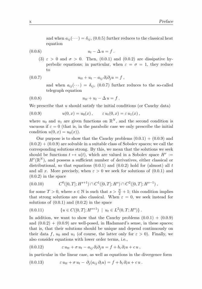
and when aij(· · · ) = δij , (0.0.5) further reduces to the classical heatequation

(0.0.6) ut −Δu = f .

(3) ε > 0 and σ > 0. Then, (0.0.1) and (0.0.2) are dissipative hy-perbolic equations; in particular, when ε = σ = 1, they reduceto

(0.0.7) utt + ut − aij ∂i∂ju = f ,

and when aij(· · · ) = δij , (0.0.7) further reduces to the so-calledtelegraph equation

(0.0.8) utt + ut −Δu = f .

We prescribe that u should satisfy the initial conditions (or Cauchy data)

(0.0.9) u(0, x) = u0(x) , ε ut(0, x) = ε u1(x) ,

where u0 and u1 are given functions on RN , and the second condition isvacuous if ε = 0 (that is, in the parabolic case we only prescribe the initialcondition u(0, x) = u0(x)).

Our purpose is to show that the Cauchy problems (0.0.1) + (0.0.9) and(0.0.2) + (0.0.9) are solvable in a suitable class of Sobolev spaces; we call thecorresponding solutions strong. By this, we mean that the solutions we seekshould be functions t �→ u(t), which are valued in a Sobolev space Hr :=Hr(RN ), and possess a sufficient number of derivatives, either classical ordistributional, so that equations (0.0.1) and (0.0.2) hold for (almost) all tand all x. More precisely, when ε > 0 we seek for solutions of (0.0.1) and(0.0.2) in the space

(0.0.10) C0([0, T ];Hs+1) ∩ C1([0, T ];Hs) ∩ C2([0, T ];Hs−1) ,

for some T > 0, where s ∈ N is such that s > N2 + 1; this condition implies

that strong solutions are also classical. When ε = 0, we seek instead forsolutions of (0.0.1) and (0.0.2) in the space

(0.0.11) {u ∈ C([0, T ];Hs+1) | ut ∈ L2(0, T ;Hs)} .In addition, we want to show that the Cauchy problems (0.0.1) + (0.0.9)and (0.0.2) + (0.0.9) are well-posed, in Hadamard’s sense, in these spaces;that is, that their solutions should be unique and depend continuously ontheir data f , u0 and u1 (of course, the latter only for ε > 0). Finally, wealso consider equations with lower order terms, i.e.,

(0.0.12) ε utt + σ ut − aij ∂i∂ju = f + bi ∂iu+ c u ,

in particular in the linear case, as well as equations in the divergence form

(0.0.13) ε utt + σ ut − ∂j(aij ∂iu) = f + bi ∂iu+ c u .

Preface xi

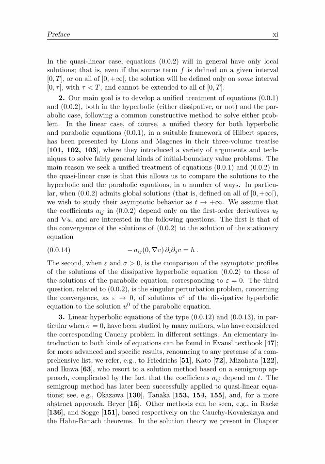
In the quasi-linear case, equations (0.0.2) will in general have only localsolutions; that is, even if the source term f is defined on a given interval[0, T ], or on all of [0,+∞[, the solution will be defined only on some interval[0, τ ], with τ < T , and cannot be extended to all of [0, T ].

2. Our main goal is to develop a unified treatment of equations (0.0.1)and (0.0.2), both in the hyperbolic (either dissipative, or not) and the par-abolic case, following a common constructive method to solve either prob-lem. In the linear case, of course, a unified theory for both hyperbolicand parabolic equations (0.0.1), in a suitable framework of Hilbert spaces,has been presented by Lions and Magenes in their three-volume treatise[101, 102, 103], where they introduced a variety of arguments and tech-niques to solve fairly general kinds of initial-boundary value problems. Themain reason we seek a unified treatment of equations (0.0.1) and (0.0.2) inthe quasi-linear case is that this allows us to compare the solutions to thehyperbolic and the parabolic equations, in a number of ways. In particu-lar, when (0.0.2) admits global solutions (that is, defined on all of [0,+∞[),we wish to study their asymptotic behavior as t → +∞. We assume thatthe coefficients aij in (0.0.2) depend only on the first-order derivatives utand ∇u, and are interested in the following questions. The first is that ofthe convergence of the solutions of (0.0.2) to the solution of the stationaryequation

(0.0.14) − aij(0,∇v) ∂i∂jv = h .

The second, when ε and σ > 0, is the comparison of the asymptotic profilesof the solutions of the dissipative hyperbolic equation (0.0.2) to those ofthe solutions of the parabolic equation, corresponding to ε = 0. The thirdquestion, related to (0.0.2), is the singular perturbation problem, concerningthe convergence, as ε → 0, of solutions uε of the dissipative hyperbolicequation to the solution u0 of the parabolic equation.

3. Linear hyperbolic equations of the type (0.0.12) and (0.0.13), in par-ticular when σ = 0, have been studied by many authors, who have consideredthe corresponding Cauchy problem in different settings. An elementary in-troduction to both kinds of equations can be found in Evans’ textbook [47];for more advanced and specific results, renouncing to any pretense of a com-prehensive list, we refer, e.g., to Friedrichs [51], Kato [72], Mizohata [122],and Ikawa [63], who resort to a solution method based on a semigroup ap-proach, complicated by the fact that the coefficients aij depend on t. Thesemigroup method has later been successfully applied to quasi-linear equa-tions; see, e.g., Okazawa [130], Tanaka [153, 154, 155], and, for a moreabstract approach, Beyer [15]. Other methods can be seen, e.g., in Racke[136], and Sogge [151], based respectively on the Cauchy-Kovaleskaya andthe Hahn-Banach theorems. In the solution theory we present in Chapter

xii Preface

2, we prefer to follow the so-called Faedo-Galerkin method, which is a gen-eralization of the method of separation of variables, and which explicitlyconstructs the solution to (0.0.12) as the limit of a sequence of functions,each of which solves an approximate version of the problem, determinedby its projection onto suitable finite-dimensional subspaces. The results weestablish for (0.0.1) when ε > 0 are not specifically dependent on the factthat the equation is hyperbolic; in fact, the Faedo-Galerkin method can bereadily adapted to obtain strong solutions of the linear parabolic equation.For general references to parabolic equations, both linear and quasi-linear,we refer, e.g., to Ladyzenshkaya, Solonnikov and Ural’tseva [86], Amann[6], Pao [131], Lunardi [107], Lieberman [96], and Krylov [83, 84], where

these equations are mostly studied in the Holder spaces Cm+α/2,2m+α(Q).For the numerical treatment of equation (2.1.1), we refer, e.g., to Meisterand Struckmeier [112].

4. The Cauchy problem for quasi-linear hyperbolic equations such as(0.0.2), as well as their counterpart in divergence form (0.0.13), has beenstudied by many authors, who have provided local (and, when possible,global, or, at least, almost global) solutions with a number of methods, in-cluding a nonlinear version of the Galerkin scheme and various versions ofthe Moser-Nash algorithm. Renouncing again to any pretense of a compre-hensive list, we refer, e.g., to the classical treatise by Courant and Hilbert[38], as well as the more recent works by Kato [72], John [66], Kichenas-samy [74], Racke [136], Sogge [151], Hormander [57], as well as Lax [88],Li Ta-Tsien [91], and Li Ta-Tsien and Wang Li-Ping [93]. In the above con-text, local solution means a solution defined on some interval [0, τ ]; almostglobal solution means a solution defined on a prescribed interval [0, T ], offinite but arbitrary length, possibly subject to some restrictions on the sizeof the data, depending on T ; global solution means a solution also definedon arbitrary intervals [0, T ], but with restrictions on the size of the data,if any, independent of T (thus, these solutions are defined on the entireinterval [0,+∞[). Finally, we also consider global bounded solutions; thatis, global solutions which remain bounded as t → +∞. In Chapter 3, wepresent a solution method based on a linearization and fixed point method,introduced by Kato [70, 71, 72], in which we apply the results for the lineartheory, developed in Chapter 2. As for the linear case, the results we estab-lish for (0.0.2), when ε > 0, are not specifically dependent on the fact thatthe equation is hyperbolic; in fact, the linearization and fixed point methodcan be adapted to obtain local, strong solutions of the quasi-linear parabolicequation

(0.0.15) ut − aij(t, x, u,∇u) ∂i∂ju = f ,

Preface xiii

as well as of the analogous equation in divergence form. Moreover, thesemethods can also be applied to other types of evolution equations, such asthe so-called dispersive equations considered in Tao [156], and Linares andPonce [97]; these include, among others, the Schrodinger and the Korteweg-de-Vries equations.

5. Not surprisingly, many more results are available on semi-linear hy-perbolic and parabolic equations; that is, equations of the form

utt −Δu = f(t, x, u,Du) ,(0.0.16)

ut −Δu = f(t, x, u,∇u) .(0.0.17)

Among the many works on this subject, we limit ourselves to cite Strauss[150], Todorova and Yordanov [159], Zheng [168], Quittner and Souplet[133], Cazenave and Haraux [24], and the references therein. Most of theseresults concern the well-posedness of the Cauchy problem for (0.0.16) or(0.0.17) in a suitable weak sense; strong solutions are then obtained byappropriate regularity theorems, and the asymptotic behavior of such weaksolutions can be studied in terms of suitable attracting sets in the phasespace; see, e.g., Milani and Koksch, [119]. In fact, we could try to develop acorresponding weak solution theory for hyperbolic and parabolic quasi-linearequations in the conservation form

(0.0.18) ε utt + σ ut − div[a(∇u)] = f ,

where a : RN → RN is monotone. However, there appears to be a strikingdifference between the hyperbolic and the parabolic situation. For the latter,i.e., when ε = 0 in (0.0.18), existence, uniqueness and well-posedness resultsfor weak solutions, at least when a is strongly monotone, are available; see,e.g., Lions [99, ch. 2, §1], and Brezis [19]. In contrast, when ε > 0 thequestion of the existence of even a local weak solution to equation (0.0.18)(that is, in the space (0.0.10) with s = 0) is, as far as we know, totally open(unless, of course, a is linear).

6. To our knowledge, there are not yet satisfactory answers to thequestion of finding sharp life-span estimates for problem (0.0.2), at least inthe functional framework we consider. On the other hand, rather preciseresults have long been available, at least for more regular solutions of thehomogeneous equation; that is, when f ≡ 0 and u0 ∈ Hs+1 ∩ W r+1,p,u1 ∈ Hs∩W r,p, for suitable integers s � N

2 +1, r < s, and p ∈ ]1, 2[. In thiscase, the situation also depends on the space dimension N ; more precisely,one obtains global existence of strong solutions if N ≥ 4, and also if N = 3if the nonlinearity satisfies an additional structural restriction, known asthe null condition. The proof of these results is based on supplementingthe direct energy estimates used to establish local solutions, with rather

xiv Preface

refined decay estimates of the solution to the linear wave equation. We referto Racke [136], and John [66], for a comprehensive survey of the resultsof, among many others, John [65], Klainerman [75, 76], Klainerman andPonce [81], as well as Klainerman [77] and Christodoulou [31], for the nullcondition.

7. The theory of quasi-linear evolution equations has many importantapplications. A non exhaustive list would include fluid dynamics (see, e.g.,Majda [108], and Nishida [126]); general relativity, and, specifically, theso-called Einstein vacuum equations (Klainerman and Christodoulou [78],and Klainerman and Nicolo [80]); wave maps (Shatah and Struwe [145],and Tao [156]); von Karman type thin plate equations (Cherrier and Milani[26, 27, 29], Chuesov and Lasiecka [33]); control and observability theory(Li [94]). Other applications, specifically of dissipative hyperbolic equations(0.0.2) with σ > 0 and ε small, include models of heat equations with delay(Li [92], Cattaneo [21], Jordan, Dai and Mickens [67], Liu [104]), where ε isa measure of the delay or heat relaxation time; Maxwell’s equations in ferro-magnetic materials (Milani [114]), where ε is a measure of the displacementcurrents, usually negligible; simple models of laser optic equations (Haus[54]), where ε is related to measures of low frequencies of the electromag-netic field; traffic flow models (Schochet [140]), where ε is a measure of thedrivers’ response time to sudden disturbances (which, one hopes, should besmall); models of random walk systems (Hadeler [53]), where ε is relatedto the reciprocal of the turning rates of the moving particles; constructionmaterials with strong internal stress-strain relations, measured by parame-ters related to the reciprocal of ε (see, e.g., Banks et al. [9, 10] for the caseof a one-dimensional elastomer); and models of time-delayed informationpropagation in economics (Ahmed and Abdusalam [2]).

8. These notes have their origin in a series of graduate courses andseminars we gave at Fudan University, Shanghai, at the Universite Pierre etMarie Curie (Paris VI), the Technische Universitat Dresden, and the Ponti-ficia Universidad Catolica of Santiago, Chile. Some of the material we coveris relatively well known, although many results, in particular on hyperbolicequations, seem to be somewhat scattered in the literature, and often sub-ordinate to other topics or applications. Other results, in particular onthe diffusion phenomenon for quasi-linear hyperbolic waves, appear to benew. Our intention is, in part, to provide an introduction to the theory ofquasi-linear evolution equations in Sobolev spaces, organizing the materialin a progression that is as gradual and natural as possible. To this end, wehave tried to put particular care in giving detailed proofs of the results wepresent; thus, if successful, our effort should give readers the necessary basisto proceed to the more specialized texts we have indicated above. In thissense, these notes are not meant to serve as an advanced PDEs textbook;

Preface xv

rather, their didactical scope and subject range is restricted to the effortof explaining, as clearly as we are able to, one possible way to study twosimple and fundamental examples of evolution equations (hyperbolic, bothdissipative or not, and parabolic) on the whole space RN . In addition, wealso hope that these notes may serve as a fairly comprehensive and self-contained reference for researchers in other areas of applied mathematicsand sciences, in which, as we have mentioned, the theory of quasi-linearevolution equations has many important applications. We should perhapsmention explicitly the fact that, given the introductory level of these notes,we have limited ourselves to present only those results that can be obtainedby resorting to one of the most standard methods for the study of equations(0.0.1) and (0.0.2); namely, that of the a priori, or energy, estimates. Ofcourse, this choice forces us to neglect other methods that are more spe-cific to the type of equation under consideration and which are extensivelystudied in more specialized texts. For example, we do not cover, but onlymention, the theory of Holder solutions of parabolic quasi-linear equations(0.0.15) (see, e.g., Krylov [83]), or the theory of weak solutions to quasi-linear first-order hyperbolic systems of conservation laws, as in (3.1.8) ofChapter 3 (see, e.g., Alinhac [5], or Serre [143, 144]), and we do not evenmention other very specific and highly refined techniques which have beendeveloped and are being developed for the study of these equations, such as,to cite a few, the theory of nonlinear semigroup (see, e.g., Beyer [15]), themethods of pseudo-differential operators (see, e.g., Taylor [157]) and of mi-crolocal analysis (see, e.g., Bony [17]). On the other hand, one can perhapsbe surprised by the extent of the results one can obtain, by means of theone and same technique; that is, the energy method. As we have stated, thismethod has, among others, the advantage of allowing us to present our re-sults in a highly unified way, and to show that, even today, classical analysisallows us to deal in a simple way, by means of standard and well-tested tech-niques, with relevant questions in the theory of PDEs of evolution, whichare still the subject of considerable study.

9. The material of these notes is organized as follows. In Chapter 1we provide a summary of the main functional analysis results we need forthe development of the theory we wish to present. In Chapter 2 we developa strong solution theory for the Cauchy problem for the linear equation(0.0.12), with existence, uniqueness, regularity, and well-posedness resultsfor both the hyperbolic equation (ε = 1, σ = 0) and the parabolic one(ε = 0, σ = 1). In Chapter 3 we construct local in time solutions to thequasi-linear equations (0.0.2) and (0.0.15), by means of a linearization andfixed-point technique, in which we apply the results on the linear equationswe established in the previous Chapter. Again, we give existence, unique-ness, regularity, and well-posedness results for both types of equation. In

xvi Preface

Chapter 4 we study the question of the extendibility of these local solu-tions to either a prefixed finite but arbitrary time interval [0, T ] (almostglobal and global existence), or to the whole interval [0,+∞[ (global andglobal bounded existence). We present an explicit example of blow-up infinite time for solutions of the quasi-linear equation (0.0.3) in one dimen-sion of space, as well as some global and almost global existence resultsfor either equation, when the data u0, u1 and f are sufficiently small. Wealso present a global existence result for the parabolic equation (0.0.15), fordata of arbitrary size. In Chapter 5 we consider the asymptotic behavior,as t → +∞, of global, bounded, small solutions of (0.0.2), both dissipa-tive hyperbolic (ε = 1) and parabolic (ε = 0), and we prove some resultson their convergence to the solution of the stationary equation (0.0.14). Inthe homogeneous case f ≡ 0, we also establish some stability estimates, onthe rate of decay to 0 of the corresponding solutions. We also give a resulton the diffusion phenomenon, which consists in showing that, when f ≡ 0,solutions of the hyperbolic equation (0.0.7) (both linear and quasi-linear)asymptotically behave as those of the parabolic equation (0.0.5) of corre-sponding type. In Chapter 6 we consider a second way in which we cancompare the hyperbolic and the parabolic problems; namely, we consider(0.0.2) as a perturbation, for small values of ε > 0, of the parabolic equation(0.0.2), with ε = 0. Denoting by uε and u0 the corresponding solutions, westudy the problem of the convergence uε → u0 as ε → 0, on compact timeintervals. We consider either intervals [0, T ] or [τ, T ], τ ∈ ]0, T [; that is, in-cluding t = 0 or not. In the former case, the convergence is singular, due tothe loss of the initial condition on ut, and we give rather precise estimates, ast and ε → 0, on the corresponding initial layer . We mention in passing thatthe estimates we establish on the difference uε − u0 allow us also to deducea global existence equivalency result between the two types of equations, inthe sense that a global solution to the parabolic equation, corresponding todata of arbitrary size, exists, if and only if global solutions to the dissipa-tive hyperbolic equation also exist, corresponding to data of arbitrary size,and ε is sufficiently small. We conclude the chapter with a global resultfor equation (0.0.2), with data of arbitrary size, when ε is sufficiently large.Lastly, in Chapter 7, we present two applications of the theory developedin the previous chapters. In the first example, we consider a model for thecomplete system of Maxwell’s equations, in which the use of suitable electro-magnetic potentials allows us to translate the first-order Maxwell’s systeminto a second-order evolution equation of the type (0.0.2). In this model,the parameters ε and σ can be interpreted as a measure, respectively, of thedisplacement and the eddy currents; in some situations, such as when theequations are considered in a ferro-magnetic medium, displacement currentsare negligible with respect to the eddy ones, and this observation leads to

Preface xvii

the question of the control of the error introduced in the model when theterm ε utt is neglected. In related situations, one is interested in periodicphenomena, with relatively low frequencies, thus leading to the question ofthe existence of solutions on the whole period of time. It is our hope thatthese questions may be addressed, at least to some extent, by the results ofthe previous chapters. In the second example, we consider two systems ofevolution equations, of hyperbolic and parabolic type, relative to a highlynonlinear elliptic system of von Karman type equations on R2m, m ≥ 2.These equations generalize the well-known equations of the same name inthe theory of elasticity, which correspond to the case m = 1, and modelthe deformation of a thin plate due to both internal and external stresses.For both types of systems we show the existence and uniqueness of local intime strong solutions, which again can be extended to almost global onesif the initial data are small enough. Even though these systems do not fitexactly in the framework of second-order evolution equations for which ourtheory is developed, their study allows us to show that the unified methodswe present can be applied to a much wider class of equations than those ofthe form (0.0.2).

10. Finally, we mention that an analogous unified theory could be con-structed for initial-boundary value problems for equation (0.0.2), in a sub-domain Ω ⊂ RN , with u subject to appropriate conditions at the boundary∂Ω of Ω, assumed to be adequately smooth. The type of results one ob-tains is qualitatively analogous, but in a different functional setting for boththe data and the solutions. Indeed, the data have to satisfy a number ofso-called compatibility conditions at {t = 0} × ∂Ω, which are different inthe hyperbolic and parabolic cases, and the integrations by parts that areusually carried out in order to establish the necessary energy estimates (seeChapter 2) would involve boundary terms that do not appear when Ω = RN .For example, in our papers [116, 117] we considered the simple case whereequation (0.0.2) is studied in a bounded domain, with homogeneous Dirich-let boundary conditions; other results can be found, e.g., in Dafermos andHrusa [40]. To discuss this topic in a meaningful degree of detail wouldrequire a whole new book; here, we limit ourselves to a reference to theabove-mentioned papers, and to the literature quoted therein, for a briefoverview of the technical issues typically encountered in this situation.

Acknowledgments. In the preparation of these notes, we have bene-fitted from the generous support of a number of agencies, including grantsfrom the Fulbright Foundation (Pontificia Universitad Catolica of Santiago,Chile, 2006), the Alexander von Humboldt Stiftung (Institut fur Analysis,Technische Universitat Dresden, 2008), and the Deutsche Forschungsgemein-schaft (TU-Dresden, 2010). We are grateful to the departments of mathe-matics of these institutions for their kind hospitality. We are also greatly

xviii Preface

indebted to Professor A. Negro of the University of Turin, Italy, to Profes-sors G. Walter and H. Volkmer of the University of Wisconsin-Milwaukee,to Professor R. Picard of the TU-Dresden, and to Professor Zheng Song-Mu of Fudan University, Shanghai, for their constant encouragement andimportant suggestions. Last, but not least, we owe special gratitude to Ms.Barbara Beeton and Ms. Jennifer Wright Sharp of the American Mathemat-ical Society Technical Support team, for their invaluable help in solving allthe TEX-nical and typographical problems involved in the production of thefinal version of this book.

Pascal Cherrier

Universite Pierre et Marie Curie, Paris

Albert Milani

University of Wisconsin - Milwaukee

List of Function Spaces

We report a list of all the function spaces we have introduced in this book. Inthe following, X is a real Banach space, Ω is a domain of RN , with boundary∂Ω, and Q = ]a, b[ ×Ω (or Q = ]a, b[ ×RN ). When Ω = RN , the explicitreference to Ω is omitted; e.g., Lp := Lp(RN ). For each space, we indicateeither the page where it has been first introduced or a reference where adefinition of the space can be found.

*****

AC([a, b];X) Space of absolutely continuous functions f : [a, b] → X(p. 62).

Cm(Ω) Space of functions f : Ω → R, which have continuous derivatives oforder up to m (p. 2).

Cmb (Ω) := {f ∈ Cm(Ω) | max

0≤j≤msupx∈Ω

|∂jf(x)| < +∞} (p. 2).

Cm0 (Ω) := {f ∈ Cm(Ω) | supp(f) is compact} (p. 2).

Cm(Ω): Space of functions which are restrictions to Ω of functions inCm(RN ) (p. 2).

Cmb (Ω): Space of functions which are restrictions to Ω of functions in

Cmb (RN ) (p. 3).

Cm,α(Ω) := {f ∈ Cm(Ω) | Hα(∂mf) < +∞}, Hα defined in (1.3.1) (p. 7).

361

362 List of Function Spaces

Cm,α(Ω) := Cm,α(Ω) ∩ Cmb (Ω) (p. 7).

Cm+α/2,2m+α(Q) :={f ∈ C(Q) | ∂k

t ∂λxf ∈ C(Q) , 2k + |λ| ≤ 2m,

Hα(∂kt ∂

λxf) < +∞ , 2k + |λ| = 2m

}, Hα defined in (1.3.4) (p. 8).

Cmb (Q) :=

{f ∈ Cb(Q) | ∂k

t ∂λxf ∈ Cb(Q) , 2k + |λ| ≤ 2m

}(p. 8).

Cm+α/2,2m+α(Q) := Cmb (Q) ∩ Cm+α/2,2m+α(Q) (p. 8).

C([a, b];X): Space of strongly continuous functions f : [a, b] → X (p. 60).

Cm([a, b];X) := {u ∈ C([a, b];X) | ∂jt u ∈ C([a, b];X) , 0 ≤ j ≤ m} (p. 64).

Cm([a, b];X,Y ) := {u ∈ C([a, b];X) | ∂mt ∈ C([a, b];Y )} (p. 64).

C([a,+∞[;X): Space of strongly continuous functions f : [a,+∞[ → X(p. 61).

Cb([a,+∞[;X): Space of strongly continuous and bounded functionsf : [a,+∞[ → X (p. 61).

Cmb ([a,+∞[;X): Space of continuously differentiable functionsf : [a,+∞[ → X, with bounded derivatives, of order up to m (p. 64).

Cmb ([a,+∞[;X,Y ) := {u ∈ Cb([a,+∞[;X) | ∂m

t u ∈ Cb([a,+∞[;Y )}(p. 64).

Cw([a, b];X): Space of weakly continuous functions f : [a, b] → X (p. 61).

D(Ω): Space of test functions in Ω (Rudin [139, ch. 6]).

D ′(Ω): Space of distributions in Ω (Rudin [139, ch. 6]).

D([a, b];X): Space of test functions f : [a, b] → X (Lions and Magenes[101, ch. 1]).

D ′(]a, b[;X) := L(D(]a, b[);X) (p. 67).

Gs(T ) := Hs+1 ×Hs × Vs−1(T ) (p. 122).

Gs(∞) := Hs+1 ×Hs × Vs−1(∞) (p. 153).

Hm(Ω) = Wm,2(Ω) := {u ∈ L2 | ∂αu ∈ L2 , |α| ≤ m} (p. 13).

Hm(Ω) := {u ∈ L∞(Ω) | ∇u ∈ Hm−1(Ω)} (m ≥ 1) (p. 14).

Hs(Ω) := (Hs�+1(Ω), Hs�(Ω))s−s� (Lions and Magenes [101, ch. 1]).

Hs(RN ) := {f ∈ S ′ | (1 + | · |2)s/2 f ∈ L2} (p. 15).

H1/2(∂Ω): Space of traces on ∂Ω of functions in H1(Ω) (p. 16).

List of Function Spaces 363

H10 (Ω) := {u ∈ H1(Ω) | u |∂Ω = 0} (p. 16).

Hm0 (Ω) := {u ∈ Hm(Ω) | ∂j

∂νju = 0 , 0 ≤ j ≤ m− 1} (p. 16).

HmΔ (Ω) := {u ∈ Hm(Ω) | (−Δ)k u ∈ H1

0 (Ω) , 0 ≤ k ≤ �m−12 �} (p. 32).

Hm∗ := {f ∈ Hm | μrf ∈ Hm−1 , 1 ≤ r ≤ N} (p. 53).

Hm(a, b;X,Y ) := Wm,2(a, b;X,Y ) (p. 68).

Hm(a, b;X) := Wm,2(a, b;X,X) (p. 68).

Hh,k(T ) := C([0, T ];Hh) ∩ C1([0, T ];Hk) (p. 348).

K := {f ∈ C1(Rm≥0;R≥0) | ∂jf ≥ 0 , 1 ≤ j ≤ m} (p. 4).

K0 := {f ∈ K | f(0) = 0} (p. 4).

K∞ := {f ∈ C(R>0;R>0) | limr→0

f(r) = +∞} (p. 4).

L(X,Y ) := {f : X → Y | f is linear continuous} (p. 5).

Lp(Ω) := {f : Ω → R | f is measurable ,∫Ω |f(x)|p dx < +∞} (up to

equivalence on sets of measure zero) (p. 9).

Lp(Γ): Lp spaces on a (N − 1)-dimensional submanifold Γ ⊂ RN (p. 9).

Lp(a, b;X) := {f : ]a, b[ → X | f is strongly measurable ,∫ ba ‖u(t)‖pX dt < +∞} (p ∈ R≥1) (p. 60).

L∞(a, b;X) := {f : ]a, b[ → X | f is strongly measurable ,sup

a<t<bess ‖u(t)‖X < +∞} (p. 60).

Pm(T ) := {u ∈ C([0, T ];Hm+1) | Du ∈ L2(0, T ;Hm)} (p. 107).

Pm(∞) := {u ∈ C([0,+∞[;Hm+1) | Du ∈ L2loc(0,+∞;Hm)} (p. 215).

Pm,b(∞) := {u ∈ Cb([0,+∞[;Hm+1) | Du ∈ L2(0,+∞;Hm)} (p. 215).

Ps(T ) := H1(0, T ;Hs+2, Hs) (p. 323).

Ph,k(T ) := {u ∈ L2(0, T ;Hh) | ut ∈ L2(0, T ;Hk)} (p. 353).

S: Schwartz’ space of rapidly decreasing functions in RN (Rudin [139,ch. 7]).

S ′: Space of tempered distributions in RN (Rudin [139, ch. 7]).

V m(RN ): The completion of Hm with respect to the norm u �→ ‖∇u‖m−1

(p. 28).

Vm(T ) := L2(0, T ;Hm+1) ∩ C([0, T ];Hm) (p. 88).

364 List of Function Spaces

Vm(∞) := L2loc(0,+∞;Hm+1) ∩ C([0,+∞[;Hm) (p. 153).

W k0 (Ω�) :=

{L2(Ω�) , if k = 0 ,

Hk(Ω�) ∩H10 (Ω�) , if k ≥ 1 .

(p. 92).

Wm,p := Wm,p(RN ) (p. 14).

Wm,p := Wm,p ∩ Cb(RN ) (p. 38).

Wm,p(a, b;X,Y ) := {u ∈ Lp(a, b;X) | u(m) ∈ Lp(a, b;Y )} (p. 68).

Wm,p(a, b;X) := Wm,p(a, b;X,X) (p. 68).

Wm,�,k(a, b) := W k,2(a, b;Hm, Hm−� k) (p. 69).

WmT (Q) := {u ∈ W 1,2(0, T ;Hm, L2) | u(T, ·) = 0} (p. 75).

WmT (Q) := {u ∈ W 1,2(−T, T ;Hm, L2) | u(−T, ·) = u(T, ·) = 0} (p. 75).

Xm(T ) := C([0, T ];Hm+1) ∩ C1([0, T ];Hm) (p. 79).

Xk,�(T ) := C([0, T ];W k+10 (Ω�)) ∩ C1([0, T ];W k

0 (Ω�)) (p. 92).

Ym(T ) := {u ∈ Xm(T ) | utt ∈ L2(0, T ;Hm−1)} (p. 79).

Yh,k(T ) := L2(0, T ;Hh) ∩ C([0, T ];H(h+k)/2) (p. 353).

Yh,k(T ) := L2(0, T ; Hh) ∩ C([0, T ]; H(h+k)/2) (p. 353).

Zm(T ) :=2⋂

j=0Cj([0, T ];Hm+1−j) (p. 88).

Zm(∞) :=2⋂

j=0Cj([0,+∞[;Hm+1−j) (p. 153).

Zm,b(∞) :=2⋂

j=0Cjb([0,+∞[;Hm+1−j) (p. 153).

Bibliography

[1] R. Adams and J. Fournier, Sobolev Spaces, 2nd ed., Academic Press, New York,2003.

[2] E. Ahmed and H. A. Abdusalam, On the Modified Black-Sholes Equation. Chaos,Solitons, and Fractals, 22 (2004), 583-587.

[3] L. Alaoglu, Weak Topologies of Normed Linear Spaces. Ann. Math., 41 (1940),252-267.

[4] S. Alinhac, Blow up for Nonlinear Hyperbolic Equations. Birkhauser, Boston, 1995.

[5] S. Alinhac, Hyperbolic Differential Equations. Springer-Verlag, New York, 2009.

[6] H. Amann, Linear and Quasilinear Parabolic Equations. Vol. I Birkhauser, Basel,1995.

[7] T. Aubin, Some Nonlinear Problems in Riemannian Geometry. Springer-Verlag,New York, 1998.

[8] T. Aubin, A Course in Differential Geometry. Graduate Series in Mathematics,14, American Mathematical Society; Providence, RI, 2000.

[9] H. T. Banks, G. A. Pinter, L. Potter, M. J. Gaitens, and L. C. Yanyo,Modelling of Nonlinear Hysteresis in Elastometers under Uniaxial Tension. J. Int.Mat. Syst. Struct., 10 (1999), 116 -134.

[10] H. T. Banks, N. G. Medin, and G. A. Pinter, Multiscale Considerations inModelling of Nonlinear Elastometers. J. Comp. Meth. in Sci. Eng., 8/2 (2007),53-62.

[11] C. Bardos, Introduction aux Problemes Hyperboliques Nonlineaires. In: Lect. NotesMath, vol. 1047; Springer-Verlag, Berlin, 1984.

[12] H. Beirao da Veiga, Perturbation Theory and Well-Posedness in Hadamard’sSense of Hyperbolic Initial-Boundary Value Problems. Nonlinear Anal., 22/10(1994), 1285–1308.

[13] M. S. Berger, On Von Karman’s Equations and the Buckling of a Thin ElasticPlate, I. Comm. Pure Appl. Math., 20 (1967), 687-719.

[14] J. Bergh and J. Lofstrom, Interpolation Spaces, an Introduction. Springer, NewYork, 1976.

365

366 Bibliography

[15] H. R. Beyer, Beyond Partial Differential Equations. Lect. Notes Math., 1898;Springer, Berlin, 2007.

[16] F. Bloom, On the Damped Nonlinear Evolution Equation wtt = (σ(w))xx − γ wt.J. Math. Anal. Appl., 96 (1983), 551-583.

[17] J. M. Bony, Analyse Microlocale et Equations d’Evolution. Sem. EDP, 2006-2007,

Exp. 20. Ecole Polytechn., Palaiseau, 2007.

[18] A. Bressan, Hyperbolic Systems of Conservation Laws: The One-DimensionalCauchy Problem. Oxford Lect. Series in Math., 20; Oxford Univ. Press, Oxford,2000.

[19] H. Brezis, Operateurs Maximaux Monotones et Semi-groupes de Contractions dansles Espaces de Hilbert. North-Holland Math. Studies, No. 5; North-Holland, Ams-terdam, 1973.

[20] L. Carleson, On Convergence and Growth of Partial Sums of Fourier Series. ActaMath., 116 (1966), 135-157.

[21] C. Cattaneo, Sulla Conduzione del Calore. Atti Sem. Mat. Fis. Univ. Modena, 3(1949). 83–101.

[22] R. Cavazzoni, On the Long Time Behavior of Solutions to Dissipative Wave Equa-tions in R

2. NoDEA, 13/2 (2006), 193-204.

[23] G. Caviglia and A. Morro, Initial-Data Dependent Conservation Laws for theTelegraph Equation. Boll. U.M.I., (7) 2-B (1988), 859-875.

[24] T. Cazenave and A. Haraux, An Introduction to Semilinear Equations of Evo-lution. Oxford Lect. Ser. in Math. and Appl., 13; Oxford Science Publ., Oxford,1998.

[25] P. Cherrier and A. Milani, Equations of Von Karman Type on Compact KahlerManifolds. Bull. Sci. Math., 2e serie, 116 (1992), 325-352.

[26] P. Cherrier and A. Milani, Parabolic Equations of Von Karman Type on Com-pact Kahler Manifolds. Bull. Sci. Math., 131 (2007), 375-396.

[27] P. Cherrier and A. Milani, Parabolic Equations of Von Karman Type on Com-pact Kahler Manifolds, II. Bull. Sci. Math., 133 (2009), 113-133.

[28] P. Cherrier and A. Milani, Decay Estimates for Quasi-Linear Evolution Equa-tions. Bull. Sci. Math., 135 (2011), 33-58.

[29] P. Cherrier and A. Milani, Hyperbolic Equations of Von Karman Type on Com-pact Kahler Manifolds. Bull. Sci. Math., 136 (2012), 19-36.

[30] R. Chill and A. Haraux, An Optimal Estimate for the Time Singular Limit ofan Abstract Wave Equation. Funkcial. Ekvak., 47/2 (2004), 277-290.

[31] D. Christodoulou, Global Solutions of Nonlinear Hyperbolic Equations for SmallInitial Data. Comm. Pure Appl. Math., 39 (1986), 267-282.

[32] K. N. Chueh, C. C. Conley, and J. Smoller, Positively Invariant Regions forSystems of Nonlinear Diffusion Equations. Ind. Univ. Math. J., 26 (1977), 372-411.

[33] I. Chuesov and I. Lasiecka, Von Karman Evolution Equations: Well-Posednessand Long-Time Dynamics. Springer-Verlag, New York, 2010.

[34] P. Ciarlet, A Justification of the von Karman Equations. Arch. Rat. Mech. Anal.,73 (1980), 349-389.

[35] P. Ciarlet, Mathematical Elasticity, Theory of Shells. North-Holland, Amsterdam,2000.

[36] P. Ciarlet and P. Rabier, Les Equations de von Karman. Springer-Verlag,Berlin, 1980.

Bibliography 367

[37] E. A. Coddington and N. Levinson, Theory of Ordinary Differential Equations.McGraw-Hill, New York, 1955.

[38] R. Courant and D. Hilbert, Methods of Mathematical Physics, vol. II. WileyClassical Eds., New York, 1989.

[39] C. Dafermos, Hyperbolic Conservation Laws in Continuum Physics, 2nd ed.,Springer-Verlag, Berlin, 2005.

[40] C. Dafermos and W. J. Hrusa, Energy Methods for Quasilinear Hyperbolic Initial-Boundary Value Problems. Arkiv Rat. Mech. An., 83/3 (1985), 267-292.

[41] R. Dautray and J. L. Lions, Analyse Mathematique et Calcul Numerique, Vol. 2.Masson, Paris, 1988.

[42] R. Dautray and J. L. Lions, Analyse Mathematique et Calcul Numerique, Vol. 5.Masson, Paris, 1988.

[43] J. Diestel and J. J. Uhl, Vector Measures. Mathematical Surveys, 15, AmericanMathematical Society; Providence, RI, 1977.

[44] G. Duvaut and J. L. Lions, Les Inequations en Mecanique et en Physique. Dunod-Gauthier-Villars, Paris, 1969.

[45] R. E. Edwards, Functional Analysis. Holt, New York, 1965.

[46] A. Erdely, W. Magnus, F. Oberhettinger, and F. G. Tricomi, Tables ofIntegral Transforms, vol. I. Bateman Man. Proj.; McGraw-Hill, New York, 1954.

[47] L. C. Evans, Partial Differential Equations. Graduate Series in Mathematics, 19,American Mathematical Society; Providence, RI, 1998.

[48] A. Favini, M. A. Horn, I. Lasiecka, and D. Tataru, Global Existence of Solu-tions to a von Karman System with Nonlinear Boundary Dissipation. J. Diff. Int.Eqs., 9/2 (1996), 267-294.

[49] A. Favini, M. A. Horn, I. Lasiecka, and D. Tataru, Addendum to the Paper“Global Existence of Solutions to a von Karman System with Nonlinear BoundaryDissipation.” J. Diff. Int. Eqs., 10/1 (1997), 197-200.

[50] G. Friedlander and M. Joshi, The Theory of Distributions. Cambridge Univ.Press, Cambridge, 1988.

[51] K. O. Friedrichs, Symmetric Hyperbolic Linear Differential Equations. Comm.Pure Appl. Math., 7 (1954), 345-392.

[52] D. Gilbarg and N. S. Trudinger, Elliptic Partial Differential Equations of SecondOrder, 2nd ed., Springer-Verlag, Berlin, 1983.

[53] K. P. Hadeler, Random Walk Systems and Reaction Telegraph Equations. InDynamical Systems and their Applications; S. v. Strien and S. V. Lunel, eds.; RoyalAcademy of the Netherlands, 1995.

[54] H. A. Haus, Waves and Fields in Optoelectronics. Prentice Hall, NJ, 1984.

[55] L. Hormander, The Fully Non-Linear Cauchy Problem with Small Data. Boll.Soc. Bras. Mat., 20 (1989), 1-27.

[56] L. Hormander, On the Fully Non-Linear Cauchy Problem with Small Data, II.In Microlocal Analysis and Nonlinear Waves. M. Beals and R. B. Melrose and J.Rauch, Eds., pp. 51-81; Springer, New York, 1991.

[57] L. Hormander, Lectures on Nonlinear Hyperbolic Partial Differential Equations.Springer-Verlag, Paris, 1997.

[58] T. Hosono and T. Ogawa, Large Time Behavior and Lp-Lq Estimate of Solutionsof 2-Dimensional Nonlinear Damped Wave Equations. J. Diff. Eqs., 203/1 (2004),82-118.

368 Bibliography

[59] L. Hsiao and T. P. Liu, Convergence to Nonlinear Diffusion Waves for Solutionsof a System of Hyperbolic Conservation Laws with Damping. Comm. Math. Phys.,143 (1992), 599-605.

[60] L. Hsiao and T. P. Liu, Nonlinear Diffusive Phenomena of Nonlinear HyperbolicSystems. Chin. Ann. Math., 14(B) (1993), 465-480.

[61] D. Huet, Decomposition Spectrale et Operateurs. Presses Univ. de France, Paris,1976.

[62] R. A. Hunt, On the Convergence of Fourier Series, Orthogonal Expansions, andtheir Continuous Analogues. Proc. Conf., Edwardsville, Ill. (1967), 235-255; South-ern Illinois Univ. Press, Carbondale, Ill.

[63] M. Ikawa, Hyperbolic Partial Differential Equations and Wave Phenomena. Trans-lations of Mathematical Monographs, 189, American Mathematical Society; Provi-dence, RI, 2000.

[64] R. Ikehata and K. Nishihara, The diffusion Phenomenon for Second Order LinearEvolution Equations. Studia Math., 158/2 (2003), 153-161.

[65] F. John, Delayed Singularity Formation in Solutions of Nonlinear Wave Equationsin Higher Dimensions. Comm. Pure Appl. Math., 29 (1976), 649-681.

[66] F. John, Nonlinear Wave Equations, Formation of Singularities. University LectureSeries, 2, American Mathematical Society; Providence, RI, 1990.

[67] P. M. Jordan, W. Dai, and R. E. Mickens, A Note on the Delayed Heat Equation:Instability with Respect to the Initial data. Mech. Res. Comm., 35 (2008), 414-420.

[68] G. Karch, Lp-decay of Solutions to Dissipative-Dispersive Perturbations of Con-servation Laws. Ann. Pol. Math., 57/1 (1997), 65-86.

[69] T. Kasuga. On Sobolev-Friedrichs’ Generalization of Derivatives. Proc. Jap. Acad.,23 (1957), 596-599.

[70] T. Kato, The Cauchy Problem for Quasi-linear Symmetric Hyperbolic Systems.Arch. Rat. Mech. Anal., 58 (1975), 181-205.

[71] T. Kato, Quasilinear Equations of Evolution, with Applications to Partial Differ-ential Equations. Lect. Notes Math. 448; Springer-Verlag, Berlin, 1975; pp. 25-70.

[72] T. Kato, Abstract Differential Equations and Nonlinear Mixed Problems. FermianLectures, Scuola Norm. Sup. Pisa, 1985.

[73] J. B. Keller and L. Ting, Periodic Vibrations of Systems Governed by NonlinearPartial Differential Equations. Comm. Pure Appl. Math., 19 (1966), 371-420.

[74] S. Kichenassamy, Nonlinear Wave Equations. Monographs in Pure Appl. Math.,194; Dekker, New York, 1996.

[75] S. Klainerman, Global Existence for Nonlinear Wave Equations. Comm. PureAppl. Math., 33 (1980), 43-101.

[76] S. Klainerman, Long Time Behavior of Solutions to Nonlinear Evolution Equa-tions. Arch. Rat. Mech. Anal., 78 (1982), 73-98.

[77] S. Klainerman, The Null Condition and Global Existence to Nonlinear Wave Equa-tions. Lect. Appl. Math., 23 (1986), 293-326.

[78] S. Klainerman and D. Christodoulou, The Global Nonlinear Stability of theMinkowski Space. Princeton Univ. Press, Princeton, NJ, 1994.

[79] S. Klainerman and A. Majda, Formation of Singularities for Wave Equations,Including the Nonlinear Vibrating String. Comm. Pure Appl. Math., 33 (1980),241-263.

Bibliography 369

[80] S. Klainerman and F. Nicolo, The Evolution Problem in General Relativity.Birkhauser, Boston, 2003.

[81] S. Klainerman and G. Ponce, Global, Small Amplitude Solutions to NonlinearEvolution Equations. Comm. Pure Appl. Math., 36/1 (1983), 133-141.

[82] H. O. Kreiss, Problems with Different Time Scales for Partial Differential Equa-tions. Comm. Pure Appl. Math., 33 (1980), 399-441.

[83] N. V. Krylov, Lectures on Elliptic and Parabolic Equations in Holder Spaces.Graduate Series in Mathematics, 12, American Mathematical Society; Providence,RI, 1996.

[84] N. V. Krylov, Lectures on Elliptic and Parabolic Equations in Sobolev Spaces.Graduate Series in Mathematics, 96, American Mathematical Society; Providence,RI, 2008.

[85] O. A. Ladyzenskaya and N. N. Ural’tseva, Linear and Quasilinear EllipticEquations. Academic Press, New York, 1968.

[86] O. A. Ladyzenskaya, V. A. Solonnikov, and N. N. Ural’tseva, Linear andQuasilinear Equations of Parabolic Type. Translations of Mathematical MonographsSeries, 23, American Mathematical Society; Providence, RI 1968.

[87] P. Lax, Development of Singularities of Solutions of Nonlinear Hyperbolic PartialDifferential Equations. J. Math. Phys., 5/5 (1964), 611-613.

[88] P. Lax, Hyperbolic Partial Differential Equations. Courant Lect. Notes, 14; CourantInst. Math., New York, 2006.

[89] Li Ya-Chun, Classical Solutions to Fully Nonlinear Wave Equations with Dissipa-tion. Chin. Ann. Math., 17A (1996), 451-466.

[90] Li Ta-Tsien, Lower Bounds for the Life-Span of Small Classical Solutions for Non-linear Wave Equations. In Microlocal Analysis and Nonlinear Waves. M. Beals andR. B. Melrose and J. Rauch, Eds., pp. 125-136; Springer, New York, 1991.

[91] Li Ta-Tsien, Global Classical Solutions for Quasilinear Hyperbolic Systems. Mas-son, Paris, 1994.

[92] Li Ta-Tsien, Nonlinear Heat Conduction with Finite Speed of Propagation. InProceedings of the China-Japan Symposium on Reaction Diffusion Equations, andtheir Applications to Computational Aspects. Li Ta-Tsien and M. Mimura and Y.Nishiura and Q. X. Ye, eds.; World Scientific, 1997.

[93] Li Ta-Tsien and Wang Li-Ping, Global Propagation of Regular Nonlinear Hyper-bolic Waves. Birkhauser, Boston, 2009.

[94] Li Ta-Tsien, Controllability and Observability for Quasi-linear Hyperbolic Systems.AIMS Appl. Math., vol. 3; Springfield, 2010.

[95] E. H. Lieb and M. Loss, Analysis, 2nd ed., Graduate Series in Mathematics, 14,American Mathematical Society; Providence, RI, 2001.

[96] G. M. Lieberman, Second Order Parabolic Differential Equations. World Scient.Publ. Co., River Edge, NJ 1996.

[97] F. Linares and G. Ponce, Introduction to Nonlinear Dispersive Equations.Springer, New York, 2009.

[98] J. L. Lions, Equations Differentielles Operationnelles, et Problemes aux Limites.Springer-Verlag, Berlin, 1961.

[99] J. L. Lions, Quelques Methodes de Resolution des Problemes aux Limites nonLineaires. Dunod-Gauthier-Villars, Paris, 1969.

370 Bibliography

[100] J. L. Lions, Perturbations Singulieres dans les Problemes aux Limites et en ControleOptimal. Lect. Notes Math. 323; Springer-Verlag, Berlin, 1973.

[101] J. L. Lions and E. Magenes, Non-Homogeneous Boundary value Problems andApplications, Vol. I. Springer-Verlag, Berlin, 1972.

[102] J. L. Lions and E. Magenes, Non-Homogeneous Boundary value Problems andApplications, Vol. II. Springer-Verlag, Berlin, 1972.

[103] J. L. Lions and E. Magenes, Non-Homogeneous Boundary value Problems andApplications, Vol. III. Springer-Verlag, Berlin, 1973.

[104] Y. K. Liu, On a Nonlinear Heat Equation with Time Delay. Eur. J. Appl. Math.,13 (2002), 321-335.

[105] Lu Yun-Guang, Hyperbolic Conservation Laws and the Compensated CompactnessMethod. Chapman & Hall, Boca Raton, FL, 2003.

[106] G. S. Ludford, Riemann’s Method of Integration: Its Extensions with an Applica-tion. Collect. Math., 6 (1953), 293-323.

[107] A. Lunardi, Analytic Semigroups and Optimal Regularity in Parabolic Equations.Birkhauser, Basel, 1995.

[108] A. Majda, Compressible Fluid Flows and Systems of Conservation Laws in SeveralSpace Dimensions. Springer-Verlag, New York, 1984.

[109] P. Marcati and K. Nishihara, The Lp-Lq Estimates of Solutions to One-Dimensional Damped Wave Equations and their Applications to the CompressibleFlow Through Porous Media. J. Diff. Eqs., 191/2 (2003), 445-469.

[110] A. Matsumura, On the Asymptotic Behavior of Solutions to Semilinear WaveEquations. Publ. RIMS Kyoto Univ., 12/1 (1976), 169-189.

[111] A. Matsumura, Global Existence and Asymptotics of the Solutions of Second OrderQuasilinear Hyperbolic Equations with First Order Dissipation Term. Publ. RIMSKyoto Univ., 13 (1977), 349-379.

[112] A. Meister and J. Struckmeier, Hyperbolic Partial Differential Equations.Vieweg, Braunschweig, 2002.

[113] M. Michael, Local and Global Solutions to Quasilinear Wave Equations via theNash-Moser Algorithm. Ph.D. Thesis, Univ. Wisc. Milwaukee, April 2009.

[114] A. Milani, The Quasi-Stationary Maxwell Equations as Singular Limits of the Com-plete Equations: The Quasilinear Case. J. Math. Anal. Appl., 102/1 (1984), 251-274.

[115] A. Milani, Global Existence via Singular Perturbation for Quasilinear EvolutionEquations. Adv. Math. Sci. Appl., 6/2 (1996), 419-444.

[116] A. Milani, Global Existence via Singular Perturbations for Quasilinear EvolutionEquations: The Initial-Boundary Value Problem. Adv. Math. Sc. Appl., 10/2(2000),735-756.

[117] A. Milani, On Singular Perturbations for Quasilinear IBV Problems. Ann. Fac.Sci. Toulouse, 9/3 (2000), 467-486.

[118] A. Milani, Almost Global Strong Solutions to Quasilinear Dissipative EvolutionEquations. Chin. Ann. Math., Ser. B, 30/1 (2009), 91-110.

[119] A. Milani and N. Koksch, An Introduction to Semiflows. Chapman & Hall, BocaRaton, FL 2005.

[120] A. Milani and Y. Shibata, On the Strong Well-Posedness of Quasilinear Hyper-bolic Initial-Boundary Value Problems. Funkcial. Ekvak., 38/3 (1995), 491-503.

Bibliography 371

[121] A. Milani and H. Volkmer, Long-Time Behavior of Small Solutions to Quasilin-ear Dissipative Hyperbolic Equations. Appl. Math., 56/5 (2011), 425-457.

[122] S. Mizohata, The Theory of Partial Differential Equations. Cambridge Univ. Press,Cambridge, 1973.

[123] B. Muckenhoupt, Equiconvergence and Almost Everywhere Convergence of Her-mite and Laguerre Series. SIAM J. Math. Anal., 1 (1970), 295-321.

[124] T. Narazaki, Lp-Lq Estimates for Damped Wave Equations, and their Applicationsto Semi-linear Problems. J. Math. Soc. Japan, 56/2 (2004), 585-626.

[125] L. Nirenberg, An Extended Interpolation Inequality. Ann. Scuola Norm. Sup. Pisa,Cl. Sci. (4), 20 (1966), 733–737.

[126] T. Nishida, Nonlinear Hyperbolic Equations and Related Topics in Fluid Dynamics.Publ. Math. d’Orsay, 78.02, Paris, 1978.

[127] K. Nishihara, Convergence Rates to Nonlinear Diffusion Waves for Solutions ofSystem of Hyperbolic Conservation Laws with Linear Damping. J. Diff. Eqns., 131(1996), 171-188.

[128] K. Nishihara, Asymptotic Behavior of Solutions of Quasilinear Hyperbolic Equa-tions with Linear Damping. J. Diff. Eqns., 137 (1997), 384-395.

[129] K. Nishihara, Lp-Lq Estimates of Solutions to the Damped Wave Equation in 3-Dimensional Space, and their Applications. Math. Zeit., 244/3 (2003), 631-649.

[130] N. Okazawa, Abstract Quasi-linear Evolution Equations of Hyperbolic Type, withApplications. Adv. Math. Sc. Appl., 7 (1996), 303-317.

[131] C. V. Pao, Nonlinear Parabolic and Elliptic Equations. Plenum Press, NY, 1992.

[132] G. Ponce, Global Existence of Small Solutions to a Class of Nonlinear EvolutionEquations. Nonlin. Anal., TMA, 9/5 (1985), 399-418.

[133] P. Quittner and P. Souplet, Superlinear Parabolic Problems. Birkhauser, Basel,2007.

[134] R. Racke, Nonhomogeneous Nonlinear Damped Wave Equations in Unbounded Do-mains. Math. Meth. Appl. Sci., 13/6 (1990), 481-491.

[135] R. Racke, Decay Rates for Solutions of Damped Systems and Generalized FourierTransforms. J. Reine Ang. Math., 412 (1990), 1-19.

[136] R. Racke, Lectures on Nonlinear Evolution Equations. Vieweg, Braunschweig,1992.

[137] M. Reissig, Klein-Gordon Type Decay Rates for Wave Equations with a Time-Dependent Dissipation. Adv. Math. Sci. Appl., 11/2 (2001), 859-891.

[138] W. Rudin, Real and Complex Analysis. McGraw-Hill, New York, 1974.

[139] W. Rudin, Functional Analysis. McGraw-Hill, New York, 1973.

[140] S. Schochet, The Instant Response Limit in Whitham’s Nonlinear Traffic FlowModel. Asympt. Anal., 1 (1988), 263-282.

[141] L. Schwartz, Theorie des Distributions. Hermann, Paris, 1998.

[142] I. Segal, Dispersion in Nonlinear Relativistic Equations, II. Ann. Sci. Ecole Norm.Sup., (4), t. 1 (1968), 458-497.

[143] D. Serre, Systemes de Lois de Conservation, I. Diderot, Paris, 1996.

[144] D. Serre, Systemes de Lois de Conservation, II. Diderot, Paris, 1996.

[145] J. Shatah and M. Struwe, Geometric Wave Equations. Courant Lect. Notes, 2;Courant Inst. Math., New York, 2000.

372 Bibliography

[146] Y. Shibata, On the Rate of Decay of Solutions to Linear Viscoelastic Equations.Math. Meth. Appl. Sci., 23 (2000), 203-226.

[147] Y. Shibata and M. Kikuchi, On the Mixed Problem for Some Quasilinear Hyper-bolic Systems with Fully Nonlinear Boundary Conditions. J. Diff. Eqs., 80/1 (1989),154-197.

[148] M. Slemrod, Damped Conservation Laws in Continuum Mechanics. In: NonlinearAnalysis and Mechanics, vol. III. Pitman, 1978.

[149] J. Smoller, Shock Waves and Reaction-Diffusion Equations, 2nd ed., Springer,New York, 1994.

[150] W. Strauss, Nonlinear Wave Equations. CBMS Reg. Conf. Ser. Math., 73. Amer-ican Mathematical Society, Providence, RI 1989.

[151] C. Sogge, Lectures on Nonlinear Wave Equations, 2nd ed., International Press,Boston, MA 2008.

[152] G. Szego, Orthogonal Polynomials. American Mathematical Society, ColloquiumPublications, Vol. XXIII; Providence, RI 1939.

[153] N. Tanaka, Global Solutions of Abstract Quasi-linear Evolution Equations of Hy-perbolic Type. Israel J. Math., 110 (1999), 219-252.

[154] N. Tanaka, A Class of Abstract Quasi-linear Evolution Equations of Second Order.J. London Math. Soc., 62 (2000), 198-212.

[155] N. Tanaka, Abstract Cauchy Problems for Quasi-linear Evolution Equations in theSense of Hadamard. Proc. London Math. Soc., 89 (2004), 123-160.

[156] T. Tao, Nonlinear Dispersive Equations. Local and Global Analysis. CBMS Series,106, American Mathematical Society; Providence, RI 2006.

[157] M. E. Taylor, Pseudodifferential Operators and Nonlinear PDEs. Birkhauser,Boston, 1991.

[158] R. Temam, Navier-Stokes Equations, Theory and Numerical Analysis, 3rd ed.,North Holland, Amsterdam, 1984.

[159] G. Todorova and B. Yordanov, Critical Exponent for a Nonlinear Wave Equa-tion with Damping. J. Diff. Eqs., 174 (2000), 464-489.

[160] H. Triebel, Interpolation Theory, Function Spaces, Differential Operators, 2nd ed.,J.A. Barth Verlag, Heidelberg, 1995.

[161] H. Volkmer, Asymptotic Expansion of L2-norms of Solutions to the Heat and Dis-sipative Wave Equations. Asympt. Anal., 67 (2010), 85-100.

[162] J. Wirth, Wave Equations with Time-Dependent Dissipation, II. Effective Dissipa-tion. J. Diff. Eqs., 232 (2007), 74-103.

[163] T. Yamazaki, Asymptotic Behavior for Abstract Wave Equations with DecayingDissipation. Adv. Diff. Eqs., 11/4 (2006), 419-456.

[164] H. Yang and A. Milani, On the Diffusion Phenomenon of Quasilinear HyperbolicWaves. Bull. Sci. Math., 124/5 (2000), 415-433.

[165] K. Yosida, Functional Analysis, 6th ed., Springer-Verlag, Berlin, 1980.

[166] E. Zeidler, Nonlinear Functional Analysis and its Applications, vol. II A. Springer-Verlag, Berlin, 1990.

[167] S. M. Zheng, Remarks on Global Existence for Nonlinear Parabolic Equations.Nonlinear Anal., 10 (1986), 107-114.

[168] S. M. Zheng, Nonlinear Evolution Equations. Monographs and Surveys in Pureand Applied Mathematics, vol. 133. Chapman & Hall, C.R.C., Boca Raton, FL 2004.

Bibliography 373

[169] S. M. Zheng and Y. M. Chen, Global Existence for Nonlinear Parabolic Equations.Chin. Ann. Math., 7B (1986), 57-73.

[170] M. Zlamal, Sur l’Equation des Telegraphistes avec un Petit Parametre. Atti Acc.Naz. Lincei, Rend. Cl. Sci. Mat. Fis. Nat., 27 (1959), 324-332.

[171] M. Zlamal, The Parabolic Equations as Limiting Case of Hyperbolic and EllipticEquations. In Differential Equations and their Applications, Proc. Equadiff I, pp.243-247. Publication House of the Czechoslovak Academy of Sciences, Prague, 1963.

Index

asymptotic profile, xi, 233, 269, 279attractor, 245

basis

Fourier, 51orthogonal, 51orthonormal, 6, 35

regular, 7, 98, 106total, 6, 90

blow up, 120, 154, 156, 157, 211

boundary conditions, xvii, 30, 90, 233,337

Cauchy data, x, 77

Cauchy problem, 77, 107, 119, 145chain of spaces, 22chain rule, 38

characteristic, 161, 166commutator

linear, 45

nonlinear, 46regularization, 46

compatibility conditions, xvii

conjugate indices, 3constituent relations, 336contraction, 120, 132, 134

convergenceweak, 5weak∗, 5

convolution, 3, 12, 141(distribution), 50, 105

corrector, 300, 321

covariant derivative, 33

critical time, 156currents

displacement, 335eddy, 335Foucault, 335

diffusion phenomenon, 233, 279, 285distribution, tempered, 14

duality, 5

eigenfunctions, 90eigenvalue, 35, 52, 160

electromagnetic fields, 335electromagnetic inductions, 335electromagnetic potentials, 337

ellipticity condition, 78, 122, 338equation

Bernoulli, 160

conservation form, 121dispersive, xiiidissipative, x, 120, 170, 175divergence form, 77, 104, 107

elliptic, 229, 233heat, x, 110, 215, 294hyperbolic, ix, 77, 119

linear, 77linearized, 119Maxwell, xvi, 294, 335Maxwell, quasi-stationary, 338

parabolic, ix, 78, 121quasi-linear, 119, 121Riccati, 211

semi-linear, xiii

375

376 Index

stationary, xi, 233, 234, 241telegraph, xvon Karman, xvii, 335, 343wave, ix

equiconvergence, 52existence

almost global, 120, 154global, 120local, 122

extension, 156extension operator, 17, 90

Faraday’s law, 336ferromagnetic media, 335fixed point, 119, 135, 146, 234formula

Duhamel, 177Faa di Bruno, 40Leibniz, 25Parseval, 14, 59Rodrigues, 51

Fourier series, 6, 106Fourier transform, 14, 51, 53Fourier’s law, 294function

absolutely continuous, 62Bessel, 52, 179Hermite, 51Holder, 7Lipschitz, 7regularized, 10Riemann, 179weakly continuous, 61

Galerkin approximation, 89, 90, 106,108

gauge relation, 338Gel’fand triple, 70genuine nonlinearity, 160

Hermite functions, 51Hermite polynomials, 51

imbeddingcompact, 5, 22, 59, 74continuous, 5, 22Sobolev, 78

inequalityGagliardo-Nirenberg, 19Gronwall, 86Hausdorff-Young, 15Holder, 11interpolation, 13, 21

Minkowski, 3Poincare, 20, 32Schwarz, 4, 11trace, 74Young, 12

initial conditions, x, 77, 107initial layer, xvi, 294, 296, 305, 321intermediate derivative, 68interpolation, 13, 68invariant interval, 154

Kronecker δ, ix

Laplace operator, 28, 30, 90, 339life span, 154, 156, 293, 333linearization, 119, 132local coordinates, 9, 16lower semi-continuity, 6

map, monotone, 336material laws, 336maximal time, 155, 156maximum principle, 121, 155, 226, 335measure, Lebesgue, 9microlocal analysis, xvmollifiers, 9, 315Moser-Nash iteration, 328multi-index, 2

length, 2

normal derivative, 16null condition, xiv, 120

operator, smoothing effect, 110orbit, 170

perturbation, 201, 245, 293, 305phase space, 81, 186, 245, 304Picard iterations, 135, 150positively invariant region, 165, 169prepared data, 296problem, well-posed, xproduct algebra, 27, 78product estimates, 24projection, 7, 91pseudo-differential operators, xv

regularity, elliptic, 31restriction, 156restriction operator, 16, 75, 90Riemann invariant, 161, 169Riemannian volume element, 9

semiflow, 81, 245

Index 377

semigroups, xvsingular convergence, 305singular perturbation, xisolution

almost global, xiiglobal, xi, xii, 120, 153global bounded, 153hyperbolic, 233local, xi, 120parabolic, 233stationary, 208, 233strong, ix, 77, 107weak, 77, 105, 121

solution kernel, 176, 215solution operator, 81solutions, bounded, xiispace

Bochner, 60Holder, 7, 8, 117intermediate, 68interpolation, 13Lebesgue, 9parabolic-Holder, 8reflexive, 5Schwartz, 14Sobolev, 13

stability, 155, 202, 219, 244strong monotonicity, 338system, dissipative, 169

theoremAlaoglu, 6Ampere, 336Caratheodory, 92extension, 75Fubini, 187, 189Tonelli, 187trace, 69

trace, 15, 16, 20, 68trace operator, 103

variation of parameters, 177

Selected Titles in This Series

135 Pascal Cherrier and Albert Milani, Linear and Quasi-linear Evolution Equations inHilbert Spaces, 2012

134 Jean-Marie De Koninck and Florian Luca, Analytic Number Theory, 2012

133 Jeffrey Rauch, Hyperbolic Partial Differential Equations and Geometric Optics, 2012

132 Terence Tao, Topics in Random Matrix Theory, 2012

131 Ian M. Musson, Lie Superalgebras and Enveloping Algebras, 2012

130 Viviana Ene and Jurgen Herzog, Grobner Bases in Commutative Algebra, 2011

129 Stuart P. Hastings and J. Bryce McLeod, Classical Methods in Ordinary DifferentialEquations, 2012

128 J. M. Landsberg, Tensors: Geometry and Applications, 2012

127 Jeffrey Strom, Modern Classical Homotopy Theory, 2011

126 Terence Tao, An Introduction to Measure Theory, 2011

125 Dror Varolin, Riemann Surfaces by Way of Complex Analytic Geometry, 2011

124 David A. Cox, John B. Little, and Henry K. Schenck, Toric Varieties, 2011

123 Gregory Eskin, Lectures on Linear Partial Differential Equations, 2011

122 Teresa Crespo and Zbigniew Hajto, Algebraic Groups and Differential Galois Theory,2011

121 Tobias Holck Colding and William P. Minicozzi, II, A Course in Minimal Surfaces,2011

120 Qing Han, A Basic Course in Partial Differential Equations, 2011

119 Alexander Korostelev and Olga Korosteleva, Mathematical Statistics, 2011

118 Hal L. Smith and Horst R. Thieme, Dynamical Systems and Population Persistence,2011

117 Terence Tao, An Epsilon of Room, I: Real Analysis, 2010

116 Joan Cerda, Linear Functional Analysis, 2010

115 Julio Gonzalez-Dıaz, Ignacio Garcıa-Jurado, and M. Gloria Fiestras-Janeiro,An Introductory Course on Mathematical Game Theory, 2010

114 Joseph J. Rotman, Advanced Modern Algebra, 2010

113 Thomas M. Liggett, Continuous Time Markov Processes, 2010

112 Fredi Troltzsch, Optimal Control of Partial Differential Equations, 2010

111 Simon Brendle, Ricci Flow and the Sphere Theorem, 2010

110 Matthias Kreck, Differential Algebraic Topology, 2010

109 John C. Neu, Training Manual on Transport and Fluids, 2010

108 Enrique Outerelo and Jesus M. Ruiz, Mapping Degree Theory, 2009

107 Jeffrey M. Lee, Manifolds and Differential Geometry, 2009

106 Robert J. Daverman and Gerard A. Venema, Embeddings in Manifolds, 2009

105 Giovanni Leoni, A First Course in Sobolev Spaces, 2009

104 Paolo Aluffi, Algebra: Chapter 0, 2009

103 Branko Grunbaum, Configurations of Points and Lines, 2009

102 Mark A. Pinsky, Introduction to Fourier Analysis and Wavelets, 2002

101 Ward Cheney and Will Light, A Course in Approximation Theory, 2000

100 I. Martin Isaacs, Algebra, 1994

99 Gerald Teschl, Mathematical Methods in Quantum Mechanics, 2009

98 Alexander I. Bobenko and Yuri B. Suris, Discrete Differential Geometry, 2008

97 David C. Ullrich, Complex Made Simple, 2008

96 N. V. Krylov, Lectures on Elliptic and Parabolic Equations in Sobolev Spaces, 2008

95 Leon A. Takhtajan, Quantum Mechanics for Mathematicians, 2008

94 James E. Humphreys, Representations of Semisimple Lie Algebras in the BGGCategory O, 2008

93 Peter W. Michor, Topics in Differential Geometry, 2008

SELECTED TITLES IN THIS SERIES

92 I. Martin Isaacs, Finite Group Theory, 2008

91 Louis Halle Rowen, Graduate Algebra: Noncommutative View, 2008

90 Larry J. Gerstein, Basic Quadratic Forms, 2008

89 Anthony Bonato, A Course on the Web Graph, 2008

88 Nathanial P. Brown and Narutaka Ozawa, C∗-Algebras and Finite-DimensionalApproximations, 2008

87 Srikanth B. Iyengar, Graham J. Leuschke, Anton Leykin, Claudia Miller, EzraMiller, Anurag K. Singh, and Uli Walther, Twenty-Four Hours of LocalCohomology, 2007

86 Yulij Ilyashenko and Sergei Yakovenko, Lectures on Analytic Differential Equations,2008

85 John M. Alongi and Gail S. Nelson, Recurrence and Topology, 2007

84 Charalambos D. Aliprantis and Rabee Tourky, Cones and Duality, 2007

83 Wolfgang Ebeling, Functions of Several Complex Variables and Their Singularities, 2007

82 Serge Alinhac and Patrick Gerard, Pseudo-differential Operators and theNash–Moser Theorem, 2007

81 V. V. Prasolov, Elements of Homology Theory, 2007

80 Davar Khoshnevisan, Probability, 2007

79 William Stein, Modular Forms, a Computational Approach, 2007

78 Harry Dym, Linear Algebra in Action, 2007

77 Bennett Chow, Peng Lu, and Lei Ni, Hamilton’s Ricci Flow, 2006

76 Michael E. Taylor, Measure Theory and Integration, 2006

75 Peter D. Miller, Applied Asymptotic Analysis, 2006

74 V. V. Prasolov, Elements of Combinatorial and Differential Topology, 2006

73 Louis Halle Rowen, Graduate Algebra: Commutative View, 2006

72 R. J. Williams, Introduction to the Mathematics of Finance, 2006

71 S. P. Novikov and I. A. Taimanov, Modern Geometric Structures and Fields, 2006

70 Sean Dineen, Probability Theory in Finance, 2005

69 Sebastian Montiel and Antonio Ros, Curves and Surfaces, 2005

68 Luis Caffarelli and Sandro Salsa, A Geometric Approach to Free Boundary Problems,2005

67 T.Y. Lam, Introduction to Quadratic Forms over Fields, 2005

66 Yuli Eidelman, Vitali Milman, and Antonis Tsolomitis, Functional Analysis, 2004

65 S. Ramanan, Global Calculus, 2005

64 A. A. Kirillov, Lectures on the Orbit Method, 2004

63 Steven Dale Cutkosky, Resolution of Singularities, 2004

62 T. W. Korner, A Companion to Analysis, 2004

61 Thomas A. Ivey and J. M. Landsberg, Cartan for Beginners, 2003

60 Alberto Candel and Lawrence Conlon, Foliations II, 2003

59 Steven H. Weintraub, Representation Theory of Finite Groups: Algebra andArithmetic, 2003

58 Cedric Villani, Topics in Optimal Transportation, 2003

57 Robert Plato, Concise Numerical Mathematics, 2003

56 E. B. Vinberg, A Course in Algebra, 2003

55 C. Herbert Clemens, A Scrapbook of Complex Curve Theory, 2003

54 Alexander Barvinok, A Course in Convexity, 2002

For a complete list of titles in this series, visit theAMS Bookstore at www.ams.org/bookstore/.

GSM/135

For additional informationand updates on this book, visit

www.ams.org/bookpages/gsm-135

www.ams.orgAMS on the Webwww.ams.org

This book considers evolution equations of hyperbolic and parabolic type. These equations are studied from a common point of view, using elementary methods, such as that of energy estimates, which prove to be quite versatile. The authors empha-size the Cauchy problem and present a unifi ed theory for the treatment of these equations. In particular, they provide local and global existence results, as well as strong well-posedness and asymptotic behavior results for the Cauchy problem for quasi-linear equations. Solutions of linear equations are constructed explicitly, using the Galerkin method; the linear theory is then applied to quasi-linear equations, by means of a linearization and fi xed-point technique. The authors also compare hyper-bolic and parabolic problems, both in terms of singular perturbations, on compact time intervals, and asymptotically, in terms of the diffusion phenomenon, with new results on decay estimates for strong solutions of homogeneous quasi-linear equa-tions of each type.

This textbook presents a valuable introduction to topics in the theory of evolution equations, suitable for advanced graduate students. The exposition is largely self-contained. The initial chapter reviews the essential material from functional analysis. New ideas are introduced along with their context. Proofs are detailed and care-fully presented. The book concludes with a chapter on applications of the theory to Maxwell’s equations and von Karman equations.