Nonlinear Riemann-Hilbert Problems and Boundary Interpolation
21
Computational Methods and Function Theory Volume 3 (2003), No. 1, 179–199 Nonlinear Riemann-Hilbert Problems and Boundary Interpolation Gunter Semmler and Elias Wegert (Communicated by Laurent Baratchart) Abstract. We study properties of solutions to non-linear Riemann-Hilbert problems with smooth compact regularly traceable target manifold. The inves- tigations focus on the dependence of solutions with positive winding numbers on additional parameters. While previous results investigated the behavior of the solutions inside the unit disk, we also pay attention to the boundary functions. As an application we consider boundary interpolation problems involving solutions to Riemann-Hilbert problems. We generalize a result by Ruscheweyh and Jones about boundary interpolation with Blaschke products. It is also shown how solutions with winding number 1 can be determined by three given points on the target manifold. Finally we formulate the problem of boundary interpolation with minimal winding number. It turns out that these problems form three subclasses, the well-posed problems constituting exactly one of them. Keywords. Riemann-Hilbert problem, interpolation problem, normal family, boundary value problem. 2000 MSC. 30E25, 30E05, 35Q15, 41A29. 1. Introduction We denote by H ∞ the Hardy space of bounded holomorphic functions in the complex unit disc D, and we let H ∞ ∩ C stand for the space of functions in H ∞ which extend continuously onto the closed disc D. The non-linear Riemann- Hilbert problem deals with finding all functions w ∈ H ∞ ∩ C which satisfy the boundary condition (1) w(t) ∈ M t for all t ∈ T on the unit circle T. Here {M t } is a given family of curves in the complex plane. Received January 25, 2003, in revised form August 22, 2003. ISSN 1617-9447/$ 2.50 c 2003 Heldermann Verlag
-
Upload
independent -
Category
Documents
-
view
1 -
download
0
Transcript of Nonlinear Riemann-Hilbert Problems and Boundary Interpolation
Computational Methods and Function TheoryVolume 3 (2003), No. 1, 179–199
Nonlinear Riemann-Hilbert Problemsand Boundary Interpolation
Gunter Semmler and Elias Wegert
(Communicated by Laurent Baratchart)
Abstract. We study properties of solutions to non-linear Riemann-Hilbertproblems with smooth compact regularly traceable target manifold. The inves-tigations focus on the dependence of solutions with positive winding numberson additional parameters. While previous results investigated the behaviorof the solutions inside the unit disk, we also pay attention to the boundaryfunctions.
As an application we consider boundary interpolation problems involvingsolutions to Riemann-Hilbert problems. We generalize a result by Ruscheweyhand Jones about boundary interpolation with Blaschke products. It is alsoshown how solutions with winding number 1 can be determined by three givenpoints on the target manifold.
Finally we formulate the problem of boundary interpolation with minimalwinding number. It turns out that these problems form three subclasses, thewell-posed problems constituting exactly one of them.
Keywords. Riemann-Hilbert problem, interpolation problem, normal family,boundary value problem.
2000 MSC. 30E25, 30E05, 35Q15, 41A29.
1. Introduction
We denote by H∞ the Hardy space of bounded holomorphic functions in thecomplex unit disc D, and we let H∞ ∩C stand for the space of functions in H∞
which extend continuously onto the closed disc D. The non-linear Riemann-Hilbert problem deals with finding all functions w ∈ H∞ ∩ C which satisfy theboundary condition
(1) w(t) ∈Mt for all t ∈ T
on the unit circle T. Here {Mt} is a given family of curves in the complex plane.
Received January 25, 2003, in revised form August 22, 2003.
ISSN 1617-9447/$ 2.50 c© 2003 Heldermann Verlag
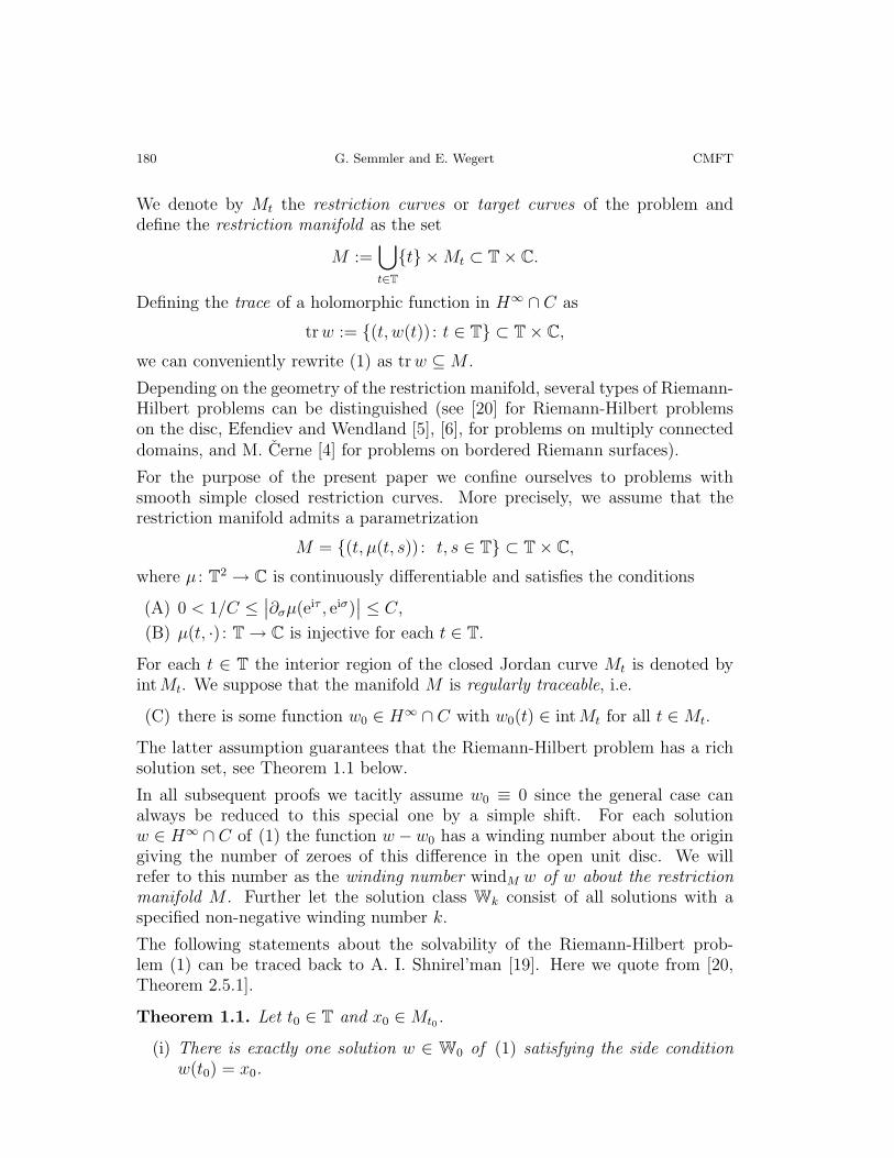
180 G. Semmler and E. Wegert CMFT
We denote by Mt the restriction curves or target curves of the problem anddefine the restriction manifold as the set
M :=⋃t∈T
{t} ×Mt ⊂ T× C.
Defining the trace of a holomorphic function in H∞ ∩ C as
trw := {(t, w(t)) : t ∈ T} ⊂ T× C,we can conveniently rewrite (1) as trw ⊆M .
Depending on the geometry of the restriction manifold, several types of Riemann-Hilbert problems can be distinguished (see [20] for Riemann-Hilbert problemson the disc, Efendiev and Wendland [5], [6], for problems on multiply connecteddomains, and M. Cerne [4] for problems on bordered Riemann surfaces).
For the purpose of the present paper we confine ourselves to problems withsmooth simple closed restriction curves. More precisely, we assume that therestriction manifold admits a parametrization
M = {(t, µ(t, s)) : t, s ∈ T} ⊂ T× C,where µ : T2 → C is continuously differentiable and satisfies the conditions
(A) 0 < 1/C ≤∣∣∂σµ(eiτ , eiσ)
∣∣ ≤ C,
(B) µ(t, ·) : T→ C is injective for each t ∈ T.
For each t ∈ T the interior region of the closed Jordan curve Mt is denoted byintMt. We suppose that the manifold M is regularly traceable, i.e.
(C) there is some function w0 ∈ H∞ ∩ C with w0(t) ∈ intMt for all t ∈Mt.
The latter assumption guarantees that the Riemann-Hilbert problem has a richsolution set, see Theorem 1.1 below.
In all subsequent proofs we tacitly assume w0 ≡ 0 since the general case canalways be reduced to this special one by a simple shift. For each solutionw ∈ H∞ ∩ C of (1) the function w − w0 has a winding number about the origingiving the number of zeroes of this difference in the open unit disc. We willrefer to this number as the winding number windM w of w about the restrictionmanifold M . Further let the solution class Wk consist of all solutions with aspecified non-negative winding number k.
The following statements about the solvability of the Riemann-Hilbert prob-lem (1) can be traced back to A. I. Shnirel’man [19]. Here we quote from [20,Theorem 2.5.1].
Theorem 1.1. Let t0 ∈ T and x0 ∈Mt0.
(i) There is exactly one solution w ∈ W0 of (1) satisfying the side conditionw(t0) = x0.
3 (2003), No. 1 Nonlinear Riemann-Hilbert Problems and Boundary Interpolation 181
(ii) Let k > 0 and z1, . . . , zk ∈ D. Then there is exactly one solution w ∈ Wk
satisfying the side condition w(t0) = x0 and the interpolation conditions
(2) w(zj) = w0(zj), j = 1, . . . , k.
In assertion (ii) the interpolation values are supposed to be the values of theholomorphic function w0 given by assumption (C). If arbitrary values are admit-ted, the situation is more complicated. In the standard case M = T
2 we obtainthe classical Nevanlinna-Pick interpolation problem.
Here we restrict ourselves to just one interpolation point, which is sufficient forthe purpose of this paper. The reader interested in the general case is referredto [22]. In order to formulate the relevant results we introduce a subset A ofbounded holomorphic functions with restricted boundary values,
A := {w ∈ H∞ : w(t) ∈ intMt a.e. on T}.For z0 ∈ D let
Y (z0) := {w(z0) : w ∈ A} ⊂ Cbe the so-called variability region. By definition, the interpolation problemw(z0) = y0 is solvable in A if and only if y0 ∈ Y (z0). More interesting is the factthat there are always solutions which also solve the Riemann-Hilbert problem.By IntY we denote the interior of a set Y ⊂ C.
Theorem 1.2 (Extremal Principle, cf. [20], Theorem 3.1.2 and Lemma 3.1.8).Let z0 ∈ D.
(i) The variability region Y (z0) is homeomorphic to the closed disc. The bound-ary ∂Y (z0) is parametrized by
∂Y (z0) = {w(z0) : w ∈W0}.(ii) Let y0 ∈ ∂Y (z0). Then there is exactly one function w ∈ A with w(z0) = y0.
This function belongs to W0, i.e. it is automatically continuous up to theboundary of the unit disc, has winding number 0 about M and satisfiesw(t) ∈Mt for all t ∈ T.
(iii) Let t0 ∈ T, x0 ∈ Mt0, and y0 ∈ IntY (z0). Then there is exactly onefunction w ∈W1 with w(z0) = y0 and w(t0) = x0.
(iv) For every k > 0 and y0 ∈ IntY (z0) there is a function w ∈ Wk withw(z0) = y0.
The first assertion makes it possible (in principle) to determine the variabilityregion Y (z0) from the solutions of the Riemann-Hilbert problem with windingnumber 0. This, in turn, can be used to solve recursively interpolation problemsof Nevanlinna-Pick type for Riemann-Hilbert problems (see [22]).
In the last section we shall investigate boundary interpolation problems wherethe interpolation points z0 are not located in D but on T. For this purposeassertion (iii) has to be considered in more detail; in particular it is essential toknow in which way the solutions depend on the interpolation data.
182 G. Semmler and E. Wegert CMFT
2. Convergence of solutions
Throughout this section two concepts of convergence will be considered. The firstone is normal convergence in D, i.e. uniform convergence on compact subsetsof D; the second one is uniform convergence in the closed unit disk D. Forfunctions harmonic in D and continuous in D, the latter is equivalent to uniformconvergence of the boundary function.
Roughly speaking, we shall show that, with fairly mild assumptions, solutionsdepend continuously on parameters in the sense of normal convergence, even ifthe interpolation point z0 ∈ D tends to the boundary of D or if the interpolationvalue y0 reaches the boundary of the variability region Y (z0).
In some applications normal convergence is too weak and convergence of theboundary function is more important than convergence in the interior of thedomain. In H∞-optimization ([10], [23]), for example, the boundary function ofthe solution corresponds to the frequency response of the system to be designed.
It is obvious that uniform convergence on D cannot take place if the windingnumber of the solutions about the target manifold changes. However, as we shallshow, in such cases the boundary functions converge uniformly on T outside aneighborhood of a finite set of points.
We begin with several lemmas on the behavior of the traces of solutions on thetarget manifold, deserving interest on their own.
Lemma 2.1. Let M ∈ C1 be a regularly traceable target manifold, and letw1 ∈Wm and w2 ∈ Wk be two solutions of the Riemann Hilbert problem. Ifw1 6= w2, the number n of intersection points of trw1 and trw2 is finite and canbe estimated by
|k −m| ≤ n ≤ k +m.
Proof. The lower estimate is purely topological: the traces of two continuousfunctions with winding numbers k and m must intersect at |k − m| points atleast. In order to prove the upper estimate we consider the following linear
Riemann-Hilbert problem wt ∈ Lt. If w1(t) and w2(t) are different, let Lt be
the straight line through these points, otherwise define Lt to be the tangent to
Mt at the point w1(t). Further, let Lt be the translations Lt := Lt − w1(t) of
Lt. The Riemann-Hilbert problem w(t) ∈ Lt is a linear homogeneous problemwith continuous coefficients and index (m+ k)/2 (note that this must not be aninteger). The function w2 − w1 is a non-trivial solution.
Now assume that the traces of w1 and w2 intersect at least at the n points(t1, y1), . . . , (tn, yn). Let
w(z) := (z − t1)−1 · · · (z − tn)−1 (w2(z)− w1(z)).
The function w is holomorphic in D and has non-tangential boundary valuesalmost everywhere on T. In order to study its boundary function we observe
3 (2003), No. 1 Nonlinear Riemann-Hilbert Problems and Boundary Interpolation 183
that the boundary function of any solution w ∈ H∞ ∩ C automatically belongsto W 1
2 (T) ([20, Theorem 2.8.1]. Since w2 − w1 vanishes at the points tj = eiτj ,j = 1, . . . , n, we have the representation
(w2 − w1)(eiτ ) =
∫ τ
τj
∂σ(w2 − w1)(eiσ) dσ.
Hardy’s inequality ([14, Theorem 5.1] then shows that the function
t 7→ (t− tj)−1(w2(t)− w1(t))
belongs to L2(T) for j = 1, . . . , n, which implies that the boundary function of wis also in L2(T). Since w is in Hp for any p < 1 we finally conclude that w ∈ H2
by Smirnov’s Theorem (cf. [13]).
The argument of t−tj is a linearly increasing function on T\{tj} and has a jumpof height π at tj. It follows that the function w ∈ H2 is a non-trivial solution ofa homogeneous linear Riemann Hilbert problem with index κ = (k + m− n)/2,which implies that κ ≥ 0, i.e. n ≤ k +m.
Corollary 2.2. If w ∈Wk with k > 0 and w0 ∈W0, then the traces of w and w0
intersect on M at exactly k points.
The traces of solutions with winding number 0 about M define a holomorphicparametrization of M in the following sense. For s ∈ T we denote by ws thesolution of the Riemann-Hilbert problem with winding number 0 which satisfiesws(1) = µ(1, s). Then
h : T2 →M, (t, s) 7→ (t, ws(t))
is a fiber-preserving homeomorphism. If we further assume that the parametriza-tion µ is chosen so that s 7→ µ(1, s) is orientation-preserving, all restrictions htof h to the fibers t = const are orientation preserving homeomorphisms of T ontothe target curves Mt.
The second component of the inverse of h is denoted by ϕ,
(3) ϕ := pr2 ◦h−1 : M → T,
where pr2 is the projection pr2(t, x) := x.
The holomorphic parametrization of M allows us to introduce a (natural) conceptof monotone behavior of continuous functions f : T → M . We say f is strictlymonotone with respect to the holomorphic parametrization of M , if there existsa branch of the argument function such that the mapping t 7→ argϕ(f(t)) iscontinuous and strictly increasing on the positively oriented arc T \ {1}. Asolution w of the Riemann-Hilbert problems is said to be strictly monotone withrespect to the holomorphic parametrization of M if the mapping t 7→ (t, w(t))has this property.
184 G. Semmler and E. Wegert CMFT
Lemma 2.3. Let M be a smooth regularly traceable target manifold. Then anysolution w ∈ H∞∩C with a positive winding number about M is strictly monotonewith respect to the holomorphic parametrization of M .
Proof. Let w ∈Wk with k > 0. Then there exists a branch of the argument sothat g : t 7→ argϕ(t, w(t)) is continuous on T \ {1} and has a jump of height 2kπat t = 1.
If g were not monotonically increasing on T\{1}, it would assume a value twice.If we now consider the values of g modulo 2π, there would exist one value whichis attained more than k times. But then the trace of w would intersect the traceof a solution with winding number 0 at more than k points, which contradictsCorollary 2.2.
The next lemma gives the clue to several results which follow.
Lemma 2.4. For any k ∈ Z the set of solutions to the Riemann-Hilbert problemwith windM w ≤ k is compact with respect to normal convergence.
Proof. 1. The set of all solutions to a Riemann-Hilbert problem with compacttarget manifold is uniformly bounded and hence a normal family. In particular,any sequence of solutions contains a subsequence (wn) which converges normallyto a function w0 ∈ H∞.
Under the hypothesis of the lemma we may assume that all solutions of thesubsequence have the same winding number, say l. We show that then w0 is asolution with m := windM w0 ≤ l.
2. For the next step it is convenient to study the situation not on M but on therectangle Q := [0, 2π]× [0, 2(l + 1)π]. The solutions wn are pulled back from Mto Q by the homeomorphism ϕ defined in (3). More precisely, we introduce thefunctions gn, n = 1, 2, . . ., on [0, 2π) by
gn(τ) := arg ϕ(eiτ , wn
(eiτ)),
and let gn(2π) = limτ→2π gn(τ) = gn(0)+2lπ. In the definition of gn a continuousbranch of the argument function is chosen so that gn(0) ∈ [0, 2π).
Note that wn can be reconstructed from gn by
wn(eiτ ) = ψ(eiτ , eign(τ)
),
where ψ := pr2 ◦h, cf. (3).
3. All functions gn are uniformly bounded, continuous, and, by Lemma 2.3,strictly monotone. By Helly’s Selection Theorem [12, Section 6.6.5, Theorem 3]the sequence (gn) contains a pointwise converging subsequence gnj . We denoteits limit by g∗ and define w∗ : T→ C by
(4) w∗(eiτ ) = ψ(eiτ , eig∗(τ)
).
3 (2003), No. 1 Nonlinear Riemann-Hilbert Problems and Boundary Interpolation 185
Since ψ is continuous, wnj(t) tends to w∗(t) for all t ∈ T. Note that g∗ and w∗
are not necessarily continuous but may have discontinuities of the first kind.
4. We extend the function w∗ harmonically into D and denote the extendedfunction again by w∗. In order to find the limit of wnj(z) as j →∞ we use Pois-son’s Integral Formula in connection with Lebesgue’s Dominated ConvergenceTheorem and see that wnj(z)→ w∗(z) for all z ∈ D.
By Step 1, the functions wn converge normally to w0, and hence w∗(z) = w0(z)if z ∈ D, which shows that the boundary function of w0 coincides with w∗ almosteverywhere on T. From equation (4) we infer that all discontinuities of theboundary function of w∗, and hence of w0, are of the first kind.
On the other hand, according to a theorem that can be traced back to Lindelof(cf. [11, Lemma 17.5.5], or [8, Chap. II, ex. 7c]), the existence of the one-sidedlimits limt→t0−0 w0(t) and limt→t0+0 w0(t) of the boundary function of w0 ∈ H∞implies that both limits coincide, and thus w0 ∈ H∞ ∩ C.
Finally, since w∗(t) ∈ Mt for all t ∈ T by construction of w∗, the function w0 isa continuous solution of the Riemann-Hilbert problem.
5. In order to estimate the winding number of w0 about M we consider themonotone function g∗. Even though w0 = w∗ is continuous, g∗ may havejumps. However, the height of every jump must be a multiple of 2π. Sinceg∗(2π)− g∗(0) = 2lπ and each jump of height 2jπ reduces the winding numberby j, the winding number of w0 about M cannot be greater than l.
Remark. The assumption that the winding number of all solutions is uniformlybounded is essential. For example, if Mt = T for all t ∈ T, the functionswn(z) = zn are solutions and converge normally to w0 ≡ 0, but this limit is nota solution.
Corollary 2.5. Any normally convergent sequence wn of solutions which satisfywindM wn ≤ k converges to a solution with windM w ≤ k.
Proof. The preceding lemma shows that any subsequence wnj of wn contains afurther (sub-)subsequence converging to a solution w with windM w ≤ k. Sincethe whole sequence wn converges normally, the limit does not depend on thechosen subsequence wnj . This implies that the entire sequence wn convergesto w.
In the next lemma we investigate what happens to the boundary functions.
Lemma 2.6. Let (wn) be a sequence of solutions to the Riemann-Hilbert problemwith windM w ≤ k which converges normally to a solution w0 with windM w = m.Then there exists a set T of at most k−m points t1, . . . , tl ∈ T and a subsequenceof (wn) which converges uniformly on any compact subset of D \ T .

186 G. Semmler and E. Wegert CMFT
Proof. We use the same notation as in the proof of Lemma 2.4. It has alreadybeen shown that the sequence (gn) contains a subsequence (gnj) which convergespointwise to a monotone function g∗.
The function g∗ is continuous at every point of the interval [0, 2π] with theexception of at most k−m points τ1, . . . , τl where it has jumps with heights thatare multiples of 2π. We set tj := exp(iτj) for j = 1, . . . , l and T := {t1, . . . , tl}.Recall that a sequence of monotone functions which converges pointwise on acompact interval to a continuous function converges uniformly. In particular,the gnj converge uniformly to g∗ on every compact subset of [0, 2π] which doesnot contain any of the points τj. Consequently, the boundary functions of wnjconverge uniformly to w∗ = w0 on all compact subsets of T \ T , and finally anestimate using Poisson’s Integral Formula yields the desired result.
3. Side conditions as parameters
After these general considerations we study in detail the behavior of solutionswith winding number 1. According to Theorem 1.2 (iii) for t0 ∈ T, x0 ∈ Mt0 ,z0 ∈ D, y0 ∈ IntY (z0) there is exactly one solution w with
(5) windM w = 1, w(t0) = x0, w(z0) = y0.
The solution w depends on the four parameters t0, x0, y0 and z0. In what followswe study what happens if t0 → t∗, x0 → x∗, y0 → y∗, and z0 → z∗. The nextthree lemmas show in which way the behavior of the solution w depends on theposition of the limits t∗, x∗, y∗, and z∗. The simplest case is considered first.
Lemma 3.1. Let t0 → t∗, x0 → x∗, y0 → y∗, z0 → z∗, where z∗ ∈ D andy∗ ∈ IntY (z∗). Then the solution w of the Riemann-Hilbert problem (1) withthe side conditions (5) converges uniformly on D to a function w∗ which is thesolution of the Riemann-Hilbert problem with
(6) windM w∗ = 1, w∗(t∗) = x∗, w∗(z∗) = y∗.
Proof. 1. The family (w) of solutions is uniformly bounded and thus it is anormal family. We can therefore select a sequence (wn) converging normally toa specific function w∗ ∈ H∞.
2. Corollary 2.5 tells us that the limit w∗ is a solution with winding number 0 or 1about M . Also, the value w∗(z∗) = limn→∞wn(z0,n) = limn→∞ y0,n = y∗ belongsto the interior of the variability region Y (z∗). By Theorem 1.2 (i), we know thatw∗ cannot have winding number 0 and so it must have winding number 1.
3. We next show that the boundary functions of wn converge uniformly on Tto the boundary function of w∗. If this were not the case, we could select asubsequence (wnk) such that the distance of wnk to w∗ in the maximum normon T is not less than a positive constant. However, it follows from Lemma 2.6,that the sequence (wnk) contains a certain subsequence (wnkj ) which converges
3 (2003), No. 1 Nonlinear Riemann-Hilbert Problems and Boundary Interpolation 187
uniformly on the whole unit circle. Since wnkj also converges normally to w∗,
the limit of this subsequence is necessarily the boundary function of w∗, whichcontradicts the above assumption.
Since uniform convergence takes places on the whole unit circle, the limit w∗
must satisfy the side condition w∗(t∗) = x∗.
4. The above argument proves that any sequence wn of solutions contains aconvergent subsequence. Since the solution w∗ is uniquely determined by theconditions (6), we obtain that the whole family (w) is convergent to w∗.
In order to illustrate this result we consider the most simple Riemann-Hilbertproblem with target curves Mt = T for all t ∈ T. Here Y (0) = D, and thesolutions with winding number 0 about M are the constant functions w(z) ≡ αwith |α| = 1. The functions
(7) w(z) = wy0(z) :=y0(1− y0)− (y0 − 1)z
1− y0 − y0(y0 − 1)z, y0 ∈ D, z ∈ D,
represent the solutions with winding number 1, wy0(1) = 1, and wy0(0) = y0.
If y0, y∗ ∈ D then the estimate
|wy0(z)− wy∗(z)| =∣∣∣∣y0(1− y0)− (y0 − 1)z
1− y0 − y0(y0 − 1)z− y∗(1− y∗)− (y∗ − 1)z
1− y∗ − y∗(y∗ − 1)z
∣∣∣∣≤ 2|y0 − y∗||1− y0||1− y∗|+ 2|y0 − y∗|+ 2|y0y
∗ − y0y∗|+ |y0y
∗||y0 − y∗|(|1− y0| − |y0||1− y0|)(|1− y∗| − |y∗||1− y∗|)
shows thatlimy0→y∗
maxz∈D|wy0(z)− wy∗(z)| = 0.
In the next lemma we consider the case where the interpolation value y0 convergesto the boundary of the range of variability.
Lemma 3.2. Let t0 → t∗, x0 → x∗, y0 → y∗, z0 → z∗, where z∗ ∈ D andy∗ ∈ ∂Y (z∗).
(i) The solution w of the Riemann-Hilbert problem (1) with the side condi-tions (5) converges normally to a function w∗ which is the solution with
windM w∗ = 0, w∗(z∗) = y∗.
(ii) If, additionally, w∗(t∗) 6= x∗, the function w converges uniformly to w∗ onevery compact subset of D \ {t∗}.
Proof. 1. As in the proof of the preceding lemma it is shown that a certainsequence of solutions wn converges normally to a solution w∗ with winding num-ber 0 or 1 about M .
2. Because z∗ ∈ D, we have w∗(z∗) = limn→∞wn(z0,n) = limn→∞ y0,n = y∗,and so w∗(z∗) belongs to the boundary of the variability region Y (z∗). Then byTheorem 1.2 (ii), w∗ must have winding number 0.

188 G. Semmler and E. Wegert CMFT
3. The uniqueness of the solution w∗ yields again the normal convergence of thewhole family (w) to w∗.
4. Let now the additional assumption w∗(t∗) 6= x∗ be satisfied. It follows fromLemma 2.6, that there is a sequence (wn) and a set T consisting of exactlyone point such that wn converges on T \ T . If T 6= {t∗} then the wn mustconverge uniformly in a neighborhood of t∗ on T. This means that we thenhave w∗(t∗) = limn→∞wn(t0,n) = limn→∞ x0,n = x∗. From this contradiction weconclude that T = {t∗}.Since the limit function and the exceptional set T are independent of the choiceof the sequence (wn), the whole family (w) of solutions converges to w∗ uniformlyon compact subsets of T\{t∗}. Assertion (ii) now follows from Poisson’s IntegralFormula.
For purposes of illustration we consider the functions (7) and let y∗ ∈ T\{1}.Then
limy0→y∗
wy0(z) =y∗ − 1− (y∗ − 1)z
1− y∗ − (1− y∗)z≡ y∗ for z ∈ T\{1}
uniformly on every closed subarc of T\{1} because
|wy0(z)− y0| =
∣∣∣∣−z(y0 − 1) + y0y0(y0 − 1)z
1− y0 − y0(y0 − 1)z
∣∣∣∣=
|z||y0 − 1|(1− |y0|2)
| − y0(y0 − 1) + 1− y0 − y0(y0 − 1)(z − 1)|
≤ |y0 − 1|(1− |y0|2)
|y0||y0 − 1||z − 1| − | − y0y0 + y0 + 1− y0|
≤ |y0 − 1|(1− |y0|2)
|y0||y0 − 1||z − 1| − 1 + |y0|2.
We remark that without the assumption w∗(t∗) 6= x∗ in Lemma 3.2 the solutionsneed not converge on the boundary. As an example we consider the functions (7)and let y0 tend to y∗ = 1 along the line arg(1 − y0) = ϑ where ϑ ∈ (−π, π) isfixed. Then for z ∈ T\{−e−2iϑ} the limit
limy0→1
arg(1−y0)=ϑ
wy0(z) = limy0→1
arg(1−y0)=ϑ
y01−y0
1−y0+ z
1−y0
1−y0+ y0z
=e−2iϑ + z
e−2iϑ + z= 1
exists. However, there is no convergence for the point z = −e−2iϑ. Dependingon the direction in which y0 approaches 1, this exceptional point can be everypoint of T.
The last result pertains to the case where the interpolation point z0 tends to theboundary of the disc.
3 (2003), No. 1 Nonlinear Riemann-Hilbert Problems and Boundary Interpolation 189
Lemma 3.3. Let t0 → t∗, x0 → x∗, y0 → y∗, z0 → z∗, where z∗ ∈ T, z∗ 6= t∗,and y∗ ∈ intMz∗. Then the function w converges uniformly on compact subsetsof D \ {z∗} to the function w∗ which is the solution with
windM w∗ = 0, w∗(t∗) = x∗.
Proof. 1. A ‘normal families’ argument proves the existence of a sequence (wn)converging normally to a solution w∗ with winding number 0 or 1.
Now Lemma 2.6 shows the existence of a subsequence of (wnk) with uniformlyconvergent boundary functions on compact subsets of T \ T , where T is emptyor a singleton.
2. In order to show that T = {z∗} we assume that T 6= {z∗}. Then theboundary functions of the subsequence (wnk) converge to the boundary functionof w∗ uniformly in a neighborhood of z∗. Using a simple estimate in Poisson’sIntegral Formula we see that wnk(z0,nk) − w∗(z0,nk) → 0 and hence also thaty0,nk = wnk(z0,nk)→ w∗(z∗) ∈Mz∗ .
On the other hand y0,nk must converge to y∗ ∈ IntY (z∗) = intMz∗ . This contra-diction shows that T = {z∗}.3. The exceptional set T = {z∗} is not empty, which, by Lemma 2.6, implies thatthe winding number of w∗ cannot be one, i.e. it must be zero. Finally, t∗ 6= z∗
implies that w∗(t∗) = limw(t0) = limx0 = x∗.
4. Since the exceptional set T and the limit function w∗ are the same for anysequence (wn), the convergence of the whole family of solutions w follows.
Remark. Recall that z0 → z∗ ∈ T implies that Y (z0) → Y (z∗) = intMz∗ ,see [20, Theorem 3.1.7] So, if y0 ∈ Y (z0), y0 → y∗ and z0 → z∗, either y∗ ∈ intMz∗
or y∗ ∈Mz∗ . The first case was considered above, in the second case the solutionneed not even converge normally. In order to give an example we take thesequence of functions wn defined by
w2n(z) =1 + 2z
2 + z, w2n+1(z) =
2z − 1
2− z,
solving the Riemann-Hilbert problem w(t) ∈ T and satisfying the side conditionswn(1) = 1. We have yn := wn(zn)→ −1 for any sequence zn ∈ D, zn → −1, butwn(0) = (−1)n/2 does not converge.
Also the solutions need not converge if z∗ = t∗. As an example consider thesame sequence of functions as before and any sequence zn ∈ D, zn → 1. Then,yn := w(zn)→ 1, but the sequence wn does not converge normally.
The above results can be extended to solutions with arbitrary winding number.We do not formulate the result in its full generality but restrict ourselves to aspecial case which shows that solutions of Riemann Hilbert problems mimic thebehavior of finite Blaschke products.

190 G. Semmler and E. Wegert CMFT
For the sake of simplicity we assume that 0 ∈ intMt for all t ∈ T. Then, forany given set of zeroes z1, . . . , zk ∈ D and each x0 ∈ Mt0 there exists a uniquelydetermined solution with windM w = k which has (simple) zeroes exactly atthe points zj and satisfies the interpolation condition w(t0) = x0. The case ofmultiple zeroes can be treated accordingly.
In the next lemma we study what happens if zeroes tend to the boundary of thecircle.
Lemma 3.4. Let x0 → x∗ ∈Mt0 and zj → z∗j with z∗j ∈ D for j = 1, . . . ,m andz∗j ∈ T \ {t0} for j = m+ 1, . . . , k. Then the solutions w with winding number kand
w(t0) = x0, w(zj) = 0, j = 1, . . . , k,
tend to the solution w∗ with winding number m and
w∗(t0) = x0, w(zj) = 0, j = 1, . . . ,m,
uniformly on all compact subsets of D \ {z∗m+1, . . . , z∗k}.
Proof. As in the proof of Lemma 3.1 we get the existence of a sequence ofsolutions wn which converges normally to a solution w∗ with winding numberp ≤ k. Since the sequence (wn) converges at the points z∗j , j = 1, . . . ,m, we havew∗(z∗j ) = 0 for j = 1, . . . ,m and hence
(8) m ≤ p ≤ k.
By Lemma 2.6 the sequence (wn) converges uniformly on any compact subset ofT \ T , where T ⊂ T consists of at most k − p points. Now all the points z∗j withj = m+ 1, . . . , k must belong to T , since otherwise w∗(z∗j ) would be zero, whichis not on Mz∗j
. Consequently p ≤ m and finally p = m because of (8).
Applying Lemma 2.6 again, we get that the exceptional set T consists exactlyof the points z∗m+1, . . . , z
∗k, and thus wn(t0) = x0 converges to w∗(t0), which
implies that w∗ has all properties mentioned in the lemma. Since there is onlyone function satisfying these conditions, any normally convergent sequence (wn)converges uniformly on T \ T to the same limit w∗. This implies that the wholefamily of solutions w converges.
4. Boundary interpolation
As an application we deal with boundary interpolation for solutions of Riemann-Hilbert problems. The first theorem generalizes a result by Ruscheweyh andJones [17], where the authors prove that for k+1 interpolation points on the unitcircle there exists a Blaschke product of degree less than or equal to k interpo-lating the given values. The problem is relevant in systems theory (see [7], [17]).We show that a similar result holds for solutions of general Riemann-Hilbertproblems.
3 (2003), No. 1 Nonlinear Riemann-Hilbert Problems and Boundary Interpolation 191
Theorem 4.1. Let M be a regularly traceable compact target manifold, and let0 ≤ τ0 < τ1 < . . . < τk < 2π, tj := eiτj , with (tj, xj) ∈ M for j = 0, . . . , k.Then there exists a solution w of the Riemann-Hilbert problem trw ⊂ M withwindM w ≤ k and
w(tj) = xj, j = 0, 1, . . . , k.
Proof. As mentioned above we can confine our considerations to the case where0 ∈ intMt for all t ∈ T. The idea of the following deduction can be understoodbest if we imagine a solution with zeroes close to the boundary of the unit disc.Such a solution behaves mostly like a solution with winding number 0, only nearthe zeroes it quickly winds around the restriction manifold. We want to locatethe zeroes in such a way that the solution meets the interpolation points whenwinding around M .
Unfortunately, the above idea does not work properly, if there is no solution withwinding number 0 that contains exactly one interpolation point. Therefore wesingle out one interpolation point and select a solution with winding number 1which has a (unique) zero near this point. We then have enough freedom tochoose this solution such that it meets only one interpolation point. A solutionof the given interpolation problem is then determined as a perturbation of thisspecific solution with winding number 1. Choosing appropriate zeroes near theboundary, all interpolation conditions can be satisfied simultaneously. Now wedevelop the details of the proof.
We suppose that the first interpolation condition is normalized so that t0 = 1 andargϕ(1, x0) = 0. Moreover we can assume that there is an m ∈ {1, . . . , k} suchthat (tm, xm) does not lie on the trace of the solution with winding number 0through the point (t0, x0).
For 0 < σm < 2π and 0 < r < 1 let wr,σm denote the solution of the Riemann-Hilbert problem
windM w = 1 w(t0) = x0 w(reiσm) = 0.
The pullback of wr,σm , defined by
gr,σm(τ) :=
0 if τ = 0,
argϕ(eiτ , wr,σm(eiτ )
)if 0 < τ < 2π,
2π if τ = 2π,
is an increasing homeomorphism of [0, 2π] onto itself. The interpolation valuesare pulled back by defining
ξj := argϕ(eiτj , xj
)∈{
[0, 2π) if j = 0, 1, . . . ,m,
(0, 2π] if j = m+ 1, . . . , k.
We now choose a positive number ε so small that
ε < minj=1,...,k0<ξj<2π
{ξj, 2π − ξj}, 4ε < min0≤j<l≤k
|τj − τl|, ε < τ1, ε < 2π − τk,
192 G. Semmler and E. Wegert CMFT
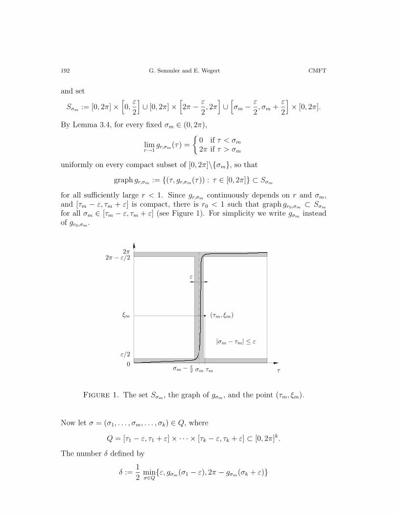
and set
Sσm := [0, 2π]×[0,ε
2
]∪ [0, 2π]×
[2π − ε
2, 2π]∪[σm −
ε
2, σm +
ε
2
]× [0, 2π].
By Lemma 3.4, for every fixed σm ∈ (0, 2π),
limr→1
gr,σm(τ) =
{0 if τ < σm2π if τ > σm
uniformly on every compact subset of [0, 2π]\{σm}, so that
graph gr,σm := {(τ, gr,σm(τ)) : τ ∈ [0, 2π]} ⊂ Sσm
for all sufficiently large r < 1. Since gr,σm continuously depends on r and σm,and [τm − ε, τm + ε] is compact, there is r0 < 1 such that graph gr0,σm ⊂ Sσmfor all σm ∈ [τm − ε, τm + ε] (see Figure 1). For simplicity we write gσm insteadof gr0,σm .
ε/2
2π − ε/22π
0τ
ξm
ε
|σm − τm| ≤ ε
σm − ε2
(τm, ξm)
σm τm
Figure 1. The set Sσm , the graph of gσm , and the point (τm, ξm).
Now let σ = (σ1, . . . , σm, . . . , σk) ∈ Q, where
Q = [τ1 − ε, τ1 + ε]× · · · × [τk − ε, τk + ε] ⊂ [0, 2π]k.
The number δ defined by
δ :=1
2minσ∈Q{ε, gσm(σ1 − ε), 2π − gσm(σk + ε)}
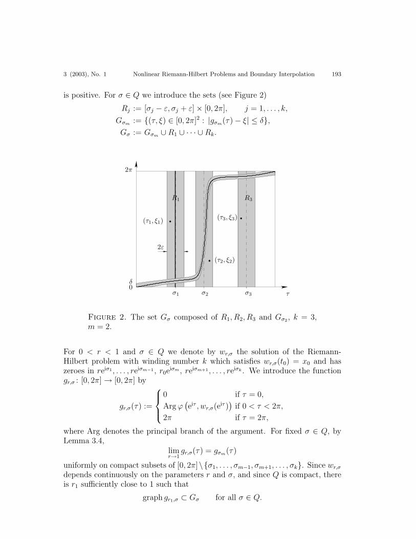
3 (2003), No. 1 Nonlinear Riemann-Hilbert Problems and Boundary Interpolation 193
is positive. For σ ∈ Q we introduce the sets (see Figure 2)
Rj := [σj − ε, σj + ε]× [0, 2π], j = 1, . . . , k,
Gσm := {(τ, ξ) ∈ [0, 2π]2 : |gσm(τ)− ξ| ≤ δ},Gσ := Gσm ∪R1 ∪ · · · ∪Rk.
δ
τ0
2π
2ε
(τ2, ξ2)
(τ1, ξ1)
σ2
(τ3, ξ3)
σ1 σ3
R1 R3
Figure 2. The set Gσ composed of R1, R2, R3 and Gσ2 , k = 3,m = 2.
For 0 < r < 1 and σ ∈ Q we denote by wr,σ the solution of the Riemann-Hilbert problem with winding number k which satisfies wr,σ(t0) = x0 and haszeroes in reiσ1 , . . . , reiσm−1 , r0eiσm , reiσm+1 , . . . , reiσk . We introduce the functiongr,σ : [0, 2π]→ [0, 2π] by
gr,σ(τ) :=
0 if τ = 0,
Argϕ(eiτ , wr,σ(eiτ )
)if 0 < τ < 2π,
2π if τ = 2π,
where Arg denotes the principal branch of the argument. For fixed σ ∈ Q, byLemma 3.4,
limr→1
gr,σ(τ) = gσm(τ)
uniformly on compact subsets of [0, 2π]\{σ1, . . . , σm−1, σm+1, . . . , σk}. Since wr,σdepends continuously on the parameters r and σ, and since Q is compact, thereis r1 sufficiently close to 1 such that
graph gr1,σ ⊂ Gσ for all σ ∈ Q.
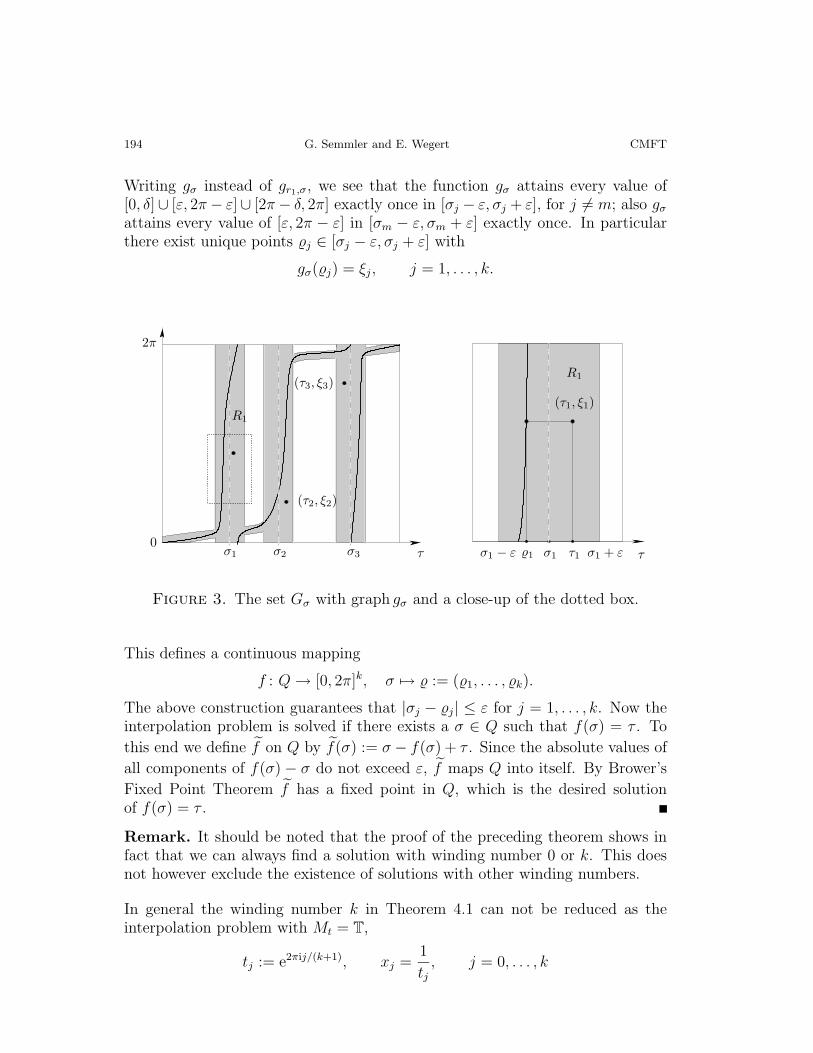
194 G. Semmler and E. Wegert CMFT
Writing gσ instead of gr1,σ, we see that the function gσ attains every value of[0, δ]∪ [ε, 2π− ε]∪ [2π− δ, 2π] exactly once in [σj − ε, σj + ε], for j 6= m; also gσattains every value of [ε, 2π − ε] in [σm − ε, σm + ε] exactly once. In particularthere exist unique points %j ∈ [σj − ε, σj + ε] with
gσ(%j) = ξj, j = 1, . . . , k.
2π
τ0
σ2 σ3σ1
R1
(τ3, ξ3)
(τ2, ξ2)
τ1
(τ1, ξ1)
R1
σ1 − ε σ1 + ε τσ1%1
Figure 3. The set Gσ with graph gσ and a close-up of the dotted box.
This defines a continuous mapping
f : Q→ [0, 2π]k, σ 7→ % := (%1, . . . , %k).
The above construction guarantees that |σj − %j| ≤ ε for j = 1, . . . , k. Now theinterpolation problem is solved if there exists a σ ∈ Q such that f(σ) = τ . To
this end we define f on Q by f(σ) := σ − f(σ) + τ . Since the absolute values of
all components of f(σ) − σ do not exceed ε, f maps Q into itself. By Brower’s
Fixed Point Theorem f has a fixed point in Q, which is the desired solutionof f(σ) = τ .
Remark. It should be noted that the proof of the preceding theorem shows infact that we can always find a solution with winding number 0 or k. This doesnot however exclude the existence of solutions with other winding numbers.
In general the winding number k in Theorem 4.1 can not be reduced as theinterpolation problem with Mt = T,
tj := e2πij/(k+1), xj =1
tj, j = 0, . . . , k
3 (2003), No. 1 Nonlinear Riemann-Hilbert Problems and Boundary Interpolation 195
shows. Nevertheless, problems involving k+1 interpolation points may very wellpossess a solution with winding number less than k. This leads to the followingproblem on minimal boundary interpolation:
For given points (tj, xj) ∈ M find the minimal winding number m of a solutionto the Riemann-Hilbert problem which satisfies w(tj) = xj for j = 0, . . . , k.
In order to get a feeling for the problem we start with three interpolation points.Comparing this situation to the problem of conformal mapping of the disk ontoa Jordan domain G we mention a classical result: if the points t1, t2, t3 ∈ T havethe same orientation as the points w1, w2, w3 ∈ ∂G, there exists a (univalent)conformal mapping w of D onto G with w(tj) = wj. In the language of Riemann-Hilbert problems this means that the boundary interpolation problem with threepoints has a solution with winding number 1.
In order to extend this result to the case of general Riemann-Hilbert problems,we introduce an orientation of point sets on M . We say that three pairwisedistinct points (t0, x0), (t1, x1), (t2, x2) ∈ M turn counterclockwise around M , ifthe triples (t0, t1, t2) and (ϕ(t0, x0), ϕ(t1, x1), ϕ(t2, x2)) have the same orientationon T (recall the definition of ϕ in (3)).
By Lemma 2.3 the existence of a solution with winding number 1 through threepoints on M implies that these points turn counterclockwise around M . Thenext theorem shows that the converse is also true.
Theorem 4.2. Let (t0, x0), (t1, x1), (t2, x2) be three points which turn counter-clockwise around M . Then there is a unique solution w ∈ H∞ ∩C with windingnumber 1 about M and
w(tj) = xj, j = 0, 1, 2.
Proof. The proof is based on a topological principle involving the winding num-ber of a continuous function on a closed contour. The lemmas of Section 3provide the necessary continuity.
1. Without loss of generality we can suppose that tj = eiτj for j = 0, 1, 2 with0 = τ0 < τ1 < τ2 < 2π and ξj = argϕ(tj, xj) are such that 0 = ξ0 < ξ1 < ξ2 < 2π.
2. It is known that the variability region Y (0) is homeomorphic to the closedunit disc. Let ω : D→ Y (0) be a homeomorphism with
ω(−i) = w−i(0)
where w−i is the solution with winding number 0 and w−i(1) = x0, and for z ∈ Tdenote by gz : [0, 2π]→ [0, 2π] the constant function
(9) gz(τ) := argϕ(eiτ , wz(eiτ ))
where wz is the solution with winding number 0 and wz(0) = ω(z) (cf. Theo-rem 1.2 (i)).
196 G. Semmler and E. Wegert CMFT
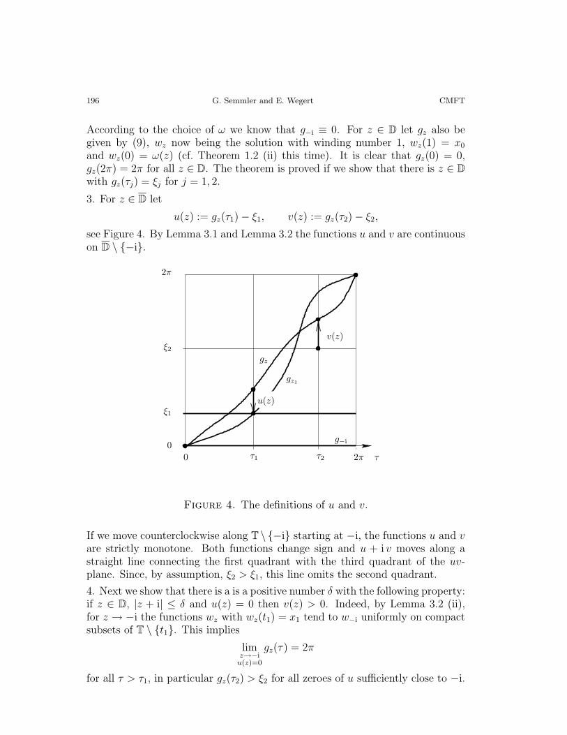
According to the choice of ω we know that g−i ≡ 0. For z ∈ D let gz also begiven by (9), wz now being the solution with winding number 1, wz(1) = x0
and wz(0) = ω(z) (cf. Theorem 1.2 (ii) this time). It is clear that gz(0) = 0,gz(2π) = 2π for all z ∈ D. The theorem is proved if we show that there is z ∈ Dwith gz(τj) = ξj for j = 1, 2.
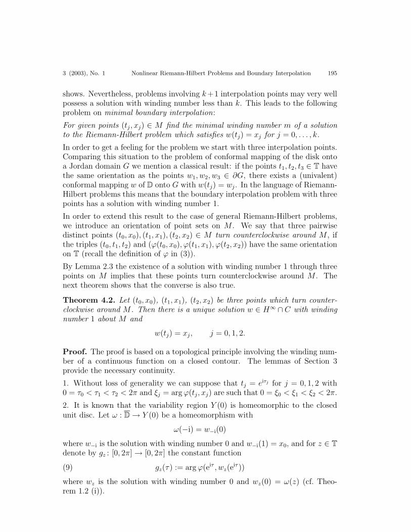
3. For z ∈ D let
u(z) := gz(τ1)− ξ1, v(z) := gz(τ2)− ξ2,
see Figure 4. By Lemma 3.1 and Lemma 3.2 the functions u and v are continuouson D \ {−i}.
ξ1
τ
ξ2
2π
gz
0
g−i0
gz1
τ2τ1
2π
u(z)
v(z)
Figure 4. The definitions of u and v.
If we move counterclockwise along T \ {−i} starting at −i, the functions u and vare strictly monotone. Both functions change sign and u + i v moves along astraight line connecting the first quadrant with the third quadrant of the uv-plane. Since, by assumption, ξ2 > ξ1, this line omits the second quadrant.
4. Next we show that there is a is a positive number δ with the following property:if z ∈ D, |z + i| ≤ δ and u(z) = 0 then v(z) > 0. Indeed, by Lemma 3.2 (ii),for z → −i the functions wz with wz(t1) = x1 tend to w−i uniformly on compactsubsets of T \ {t1}. This implies
limz→−iu(z)=0
gz(τ) = 2π
for all τ > τ1, in particular gz(τ2) > ξ2 for all zeroes of u sufficiently close to −i.

3 (2003), No. 1 Nonlinear Riemann-Hilbert Problems and Boundary Interpolation 197
5. Let D := {z ∈ D : |z + i| > δ}. The boundary K of D consists of two circulararcs – an arc with center −i and radius δ, and a subarc of T which does notcontain −i. The mapping ψ : D → C, z 7→ u(z) + i v(z) is continuous on theclosure of D. The image of the contour K consists of a segment L connectinga certain point a in the first quadrant with a point b in third quadrant, and acurve connecting b with a and omitting the set {u+ i v : v ≤ 0} (see Figure 5).
−i
D
D
K
z
u
b
a
v
Figure 5. The contour K and its image.
Consequently, the winding number of ψ(K) about zero is ±1 (the sign dependson the orientation of the homeomorphism ω), and by a well-known topologicalprinciple ψ must have a zero z ∈ D, i.e. gz(τ1) = ξ1, gz(τ2) = ξ2.
The uniqueness of the solution follows from Lemma 2.1.
If the number of interpolation points is greater than three the situation is morecomplicated. Even in the standard case M = T
2, where the solutions of theRiemann-Hilbert problem are the finite Blaschke products, we have not been ableto find a (reasonable) criterion which allows the determination of the minimaldegree of the interpolating Blaschke products, but at least we would like tomention some particular results.
Using linearization techniques and the Fredholm theory of linear Riemann-Hilbertproblems we have shown that there are three qualitatively different types ofboundary interpolation problems. The classification depends on a relation be-tween the number k of interpolation points and the minimal winding number mof their solution (note the different meaning of k compared with the statementsabove).
(i) (Fragile problems.) If 0 ≤ m < (k − 1)/2, there exist small perturbationsof the interpolation values such that the solution of the perturbed problemhas a minimal winding number greater than m.
198 G. Semmler and E. Wegert CMFT
(ii) (Rigid problems.) If m = (k− 1)/2, then for all sufficiently small perturba-tions the perturbed problem has a unique solution with minimal windingnumber equal to m.
(iii) (Flexible problems.) If (k − 1)/2 < m ≤ k − 1, the solution with minimalwinding number is not unique.
For all k > 1 the fragile problems form a thin set. If k is even, there are no rigidproblems. If k is odd, rigid and flexible problems are generic.
Fragile and flexible problems are not well-posed, which might be the reason whythe problem in Theorem 4.1 has not been extensively studied in the literatureeven for Blaschke products (see [2],[3]). D. Sarason [18] proposed a modifica-tion of the problem in order to make it well-posed. But indeed rigid minimalinterpolation problems are generic and well-posed.
We would like to encourage research on the following three problems, which havenot yet been solved to the best of our knowledge.
1. Find a criterion or an algorithm to decide if a given problem is rigid.
2. Find a constructive method to determine the solution of rigid problems.
3. Find an efficient criterion or an algorithm to classify a given problem.
Acknowledgement. We would like to thank the referee for valuable sugges-tions and comments. In particular, his (or her) critical remarks eliminated aninsufficiency in the proof of Theorem 4.2.
References
1. P. Duren, Theory of Hp Spaces, Academic Press, New York and London, 1970.2. D. G. Cantor and R. R. Phelps, An elementary interpolation theorem, Proc. Amer. Math.
Soc. 16 (1965), 623–525.3. G. T. Cargo, Blaschke products and singular inner functions with prescribed boundary
values, J. Math. Anal. Appl. 71 (1979), 287–296.4. M. Cerne, Nonlinear Riemann-Hilbert problem for bordered Riemann surfaces, to appear
in Amer. J. Math.5. M. A. Efendiev and W. L. Wendland, Nonlinear Riemann-Hilbert problems without
transversality, Math. Nachr. 183 (1997), 73–89.6. , Nonlinear Riemann-Hilbert problems for doubly connected domains and closed
boundary data, Topol. Methods Nonlinear Anal. 17 (2001), 111–124.7. G. Feyh, W. B. Jones, and C. T. Mullis, An extension of the Schur algorithm for frequency
transformations, in: Linear Circuits, Systems and Signal Processing, Sel. Pap. 8th Int.Symp. Math. Theory Networks Syst., Phoenix/Ariz. 1987 (1988), 191–196.
8. J. B. Garnett, Bounded Analytic Functions, Academic Press, New York, 1981.9. G. M. Golusin, Geometrische Funktionentheorie, VEB Deutscher Verlag der Wissen-
schaften 1957; German translation of: G. M. Golusin, Geometriqeska� teori� funkci�
kompleksnogo peremennogo , GITTL, M.-L., 1952.10. J. W. Helton and O. Merino, Classical Control Using H∞ Methods — Theory, Optimiza-
tion, and Design, Philadelphia, SIAM 1998, 292 pp.11. E. Hille, Analytic Function Theory, Vol. 2, Chelsea Publishing Company, New York, 1962.
3 (2003), No. 1 Nonlinear Riemann-Hilbert Problems and Boundary Interpolation 199
12. A. N. Kolmogorov and S. V. Fomin, Reelle Funktionen und Funktionalanalysis, DeutscherVerlag der Wissenschaften, 1975; German translation of, A. N. Kolmogorov i S. V. Fomin ,�lementy teorii funkci� i funkcional~nogo analiza , Izd. Nauka, Moskva , 1972.
13. P. Koosis, Lectures on Hp Spaces, London Math. Soc. Lect. Notes Series No. 40, CambridgeUniv. Press, London, 1980.
14. A. Kufner, Weighted Sobolev Spaces, Teubner, Leipzig, 1980.15. M. H. A. Newman, Elements of the Topology of Plane Sets of Points, Dover Publications,
1992.16. M. Rosenblum and J. Rovnyak, Topics in Hardy Classes and Univalent Functions,
Birkhauser, Basel, 1994.17. S. Ruscheweyh and W. B. Jones, Blaschke product interpolation and its application to the
design of digital filters, Constr. Approx. 3 (1987), 405–409.18. D. Sarason, Nevanlinna-Pick interpolation with boundary data, Integral Equations Oper.
Theory 30 2 (1998), 231–250.19. A. I. Shnirel’man, The degree of a quasi-linearlike mapping and the nonlinear Hilbert
problem (in Russian), Mat. Sb. 89 3 (1972), 366–389; English transl.: Math. USSR Sbornik18 (1974), 373–396.
20. E. Wegert, Nonlinear Boundary Value Problems for Holomorphic Functions and SingularIntegral Equations, Akademie Verlag, Berlin, 1992.
21. , Nonlinear Riemann-Hilbert problems — history and perspectives, in: N. Papa-michael et al. (eds.), Computational Methods in Function Theory, World Scientific Pub-lishing Company, 1999, 583–615.
22. , Interpolation by holomorphic functions with restricted boundary values, in: Th.Vougiouklis, Proceed. Int. Congr. Vissa-Orestiada Sept. 2000, Hadronic Press, 2001, 61–79.
23. M. A. Whittlesey, Polynomial hulls and H∞ control for a hypoconvex constraint, Math.Ann. 317 4 (2000), 677–701.
Gunter Semmler E-mail: [email protected]: Institute of Applied Analysis, University of Mining and Technology, 09596 Freiberg,Germany.
Elias Wegert E-mail: [email protected]: Institute of Applied Analysis, University of Mining and Technology, 09596 Freiberg,Germany.