Ursinus College Ursinus College

Digital Commons @ Ursinus College Digital Commons @ Ursinus College

Calculus Transforming Instruction in Undergraduate

Mathematics via Primary Historical Sources (TRIUMPHS)

Winter 2020

Beyond Riemann Sums: Fermat's Method of Integration Beyond Riemann Sums: Fermat's Method of Integration

Dominic Klyve Central Washington University, Dominic.Klyve@cwu.edu

Follow this and additional works at: https://digitalcommons.ursinus.edu/triumphs_calculus

Click here to let us know how access to this document benefits you. Click here to let us know how access to this document benefits you.

Recommended Citation Recommended Citation Klyve, Dominic, "Beyond Riemann Sums: Fermat's Method of Integration" (2020). Calculus. 12. https://digitalcommons.ursinus.edu/triumphs_calculus/12

This Course Materials is brought to you for free and open access by the Transforming Instruction in Undergraduate Mathematics via Primary Historical Sources (TRIUMPHS) at Digital Commons @ Ursinus College. It has been accepted for inclusion in Calculus by an authorized administrator of Digital Commons @ Ursinus College. For more information, please contact aprock@ursinus.edu.

Beyond Riemann Sums: Fermat’s method of integration

Dominic Klyve∗

February 8, 2020

Introduction

Finding areas of shapes, especially shapes with curved boundaries, has challenged mathematicians for

thousands of years. Today calculus students learn to graph functions, approximate the area with

rectangles of the same width, and use “Riemann Sums” to approximate the area under a curve (or, by

taking limits, to find it exactly). Centuries before Riemann used this method, and a generation before

Newton and Leibniz discovered calculus, seventeenth-century lawyer (and math fan) Pierre de Fermat

(1607–1665) used a similar method, with an interesting twist that let the widths of the rectangles get

larger as x grows. In this Primary Source Project, we will explore Fermat’s method.

Part 1: On “quadrature”

It’s worth noting that Fermat thought of area slightly differently than we usually do today. Following

the work of Ancient Greek mathematicians, his goal was “quadrature” – finding or constructing a

rectangular shape with the same area as that of the shape he wanted to measure. In English, this is

often called “squaring”, so that “squaring the circle” means to construct, using the tools of geometry,

a square with the same area as a given circle.

During Fermat’s time, there were not many curves under which mathematicians could find the area

precisely. Fermat was particularly interested in exploring not individual curves, but whole classes of

them that could be studied with the same means. In his Treatise on Quadrature1 (c. 1659), one such

class that he studied were curves that today we would write as functions of the form y = 1xn . His primary

method of finding these areas closely resembled the method of Riemann Sums, which was not introduced

until almost two centuries later.2 Fermat wanted to approximate the area under the curve with a series

∗Department of Mathematics, Central Washington University, Ellensburg, WA 98926; dominic.klyve@cwu.edu.1The full title is quite long: De aequationum localium transmutatione et emendatione ad multimodam curvilineorum

inter se vel cum rectilineis comparationem, cui annectitur proportionis geometricae in quadrandis infinitis parabolis et

hyperbolis usus, which Mahoney translates as “On the transformation and alteration of local equations for the purpose of

variously comparing curvilinear figures among themselves or to rectilinear figures, to which is attached the use of geometric

proportions in squaring an infinite number of parabolas and hyperbolas”. [?]2Bernhard Riemann (1826–1866) developed the notion of what we now call “Riemann Sums”, but they didn’t originally

look like the version we teach in Calculus today. Augustin-Louis Cauchy (1789–1857) is generally credited with being the

first to define the definite integral in our modern formulation.

1

of rectangles whose areas lay in geometric proportion. First, however, he needed to establish some basic

facts about such a series:

∞∞∞∞∞∞∞∞∞∞∞∞∞∞∞∞∞∞∞∞∞∞∞∞∞∞∞∞∞∞∞∞∞∞∞∞∞∞∞∞

Given any geometric proportion the terms of which decrease indefinitely, the difference between

two consecutive terms of this progression is to the smaller term as the greater one is to the sum

of all following terms.

∞∞∞∞∞∞∞∞∞∞∞∞∞∞∞∞∞∞∞∞∞∞∞∞∞∞∞∞∞∞∞∞∞∞∞∞∞∞∞∞

Let’s try to make sense of this. In a geometric proportion, any two consecutive terms have a constant

ratio. Consider the series∞∑n=0

1

rn= 1 +

1

r+

1

r2+ · · · .

Task 1 Is this a “ geometric proportion the terms of which decrease indefinitely”, as Fermat required?

Why or why not?

Task 2 The latter part of Fermat’s claim is an equality of two ratios. Write it out, and then solve for the

the value of the infinite series. Does the solution look familiar?

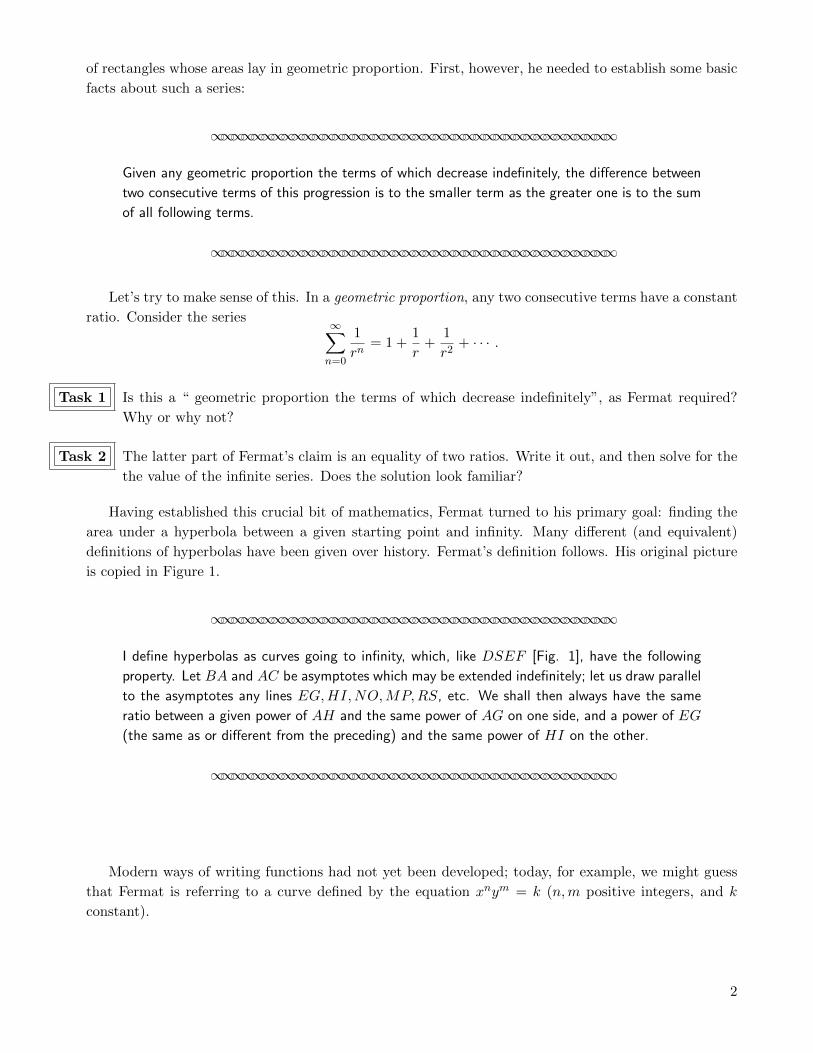
Having established this crucial bit of mathematics, Fermat turned to his primary goal: finding the

area under a hyperbola between a given starting point and infinity. Many different (and equivalent)

definitions of hyperbolas have been given over history. Fermat’s definition follows. His original picture

is copied in Figure 1.

∞∞∞∞∞∞∞∞∞∞∞∞∞∞∞∞∞∞∞∞∞∞∞∞∞∞∞∞∞∞∞∞∞∞∞∞∞∞∞∞

I define hyperbolas as curves going to infinity, which, like DSEF [Fig. 1], have the following

property. Let BA and AC be asymptotes which may be extended indefinitely; let us draw parallel

to the asymptotes any lines EG,HI,NO,MP,RS, etc. We shall then always have the same

ratio between a given power of AH and the same power of AG on one side, and a power of EG

(the same as or different from the preceding) and the same power of HI on the other.

∞∞∞∞∞∞∞∞∞∞∞∞∞∞∞∞∞∞∞∞∞∞∞∞∞∞∞∞∞∞∞∞∞∞∞∞∞∞∞∞

Modern ways of writing functions had not yet been developed; today, for example, we might guess

that Fermat is referring to a curve defined by the equation xnym = k (n,m positive integers, and k

constant).

2

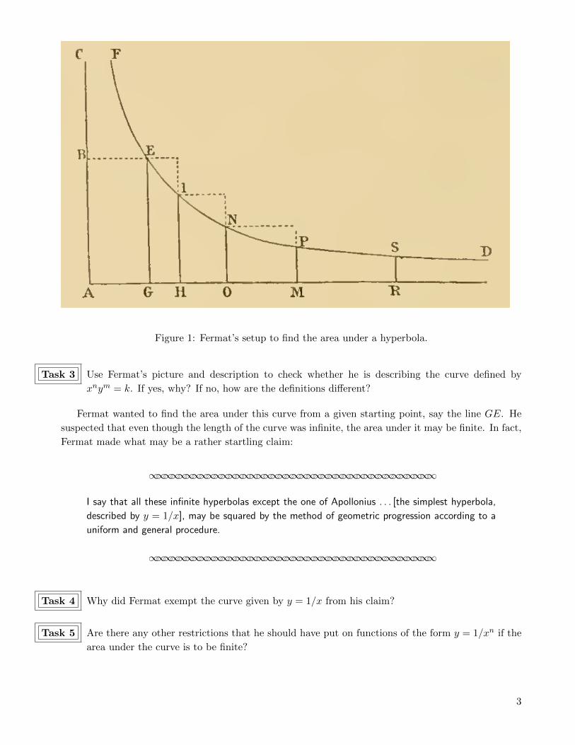
Figure 1: Fermat’s setup to find the area under a hyperbola.

Task 3 Use Fermat’s picture and description to check whether he is describing the curve defined by

xnym = k. If yes, why? If no, how are the definitions different?

Fermat wanted to find the area under this curve from a given starting point, say the line GE. He

suspected that even though the length of the curve was infinite, the area under it may be finite. In fact,

Fermat made what may be a rather startling claim:

∞∞∞∞∞∞∞∞∞∞∞∞∞∞∞∞∞∞∞∞∞∞∞∞∞∞∞∞∞∞∞∞∞∞∞∞∞∞∞∞

I say that all these infinite hyperbolas except the one of Apollonius . . . [the simplest hyperbola,

described by y = 1/x], may be squared by the method of geometric progression according to a

uniform and general procedure.

∞∞∞∞∞∞∞∞∞∞∞∞∞∞∞∞∞∞∞∞∞∞∞∞∞∞∞∞∞∞∞∞∞∞∞∞∞∞∞∞

Task 4 Why did Fermat exempt the curve given by y = 1/x from his claim?

Task 5 Are there any other restrictions that he should have put on functions of the form y = 1/xn if the

area under the curve is to be finite?

3

Fermat started to set up his solution as follows:

∞∞∞∞∞∞∞∞∞∞∞∞∞∞∞∞∞∞∞∞∞∞∞∞∞∞∞∞∞∞∞∞∞∞∞∞∞∞∞∞

Imagine the terms of a geometric progression, extended in infinitium, of which the first is AG,

the second AH, the third AO, etc., in infinitum,

∞∞∞∞∞∞∞∞∞∞∞∞∞∞∞∞∞∞∞∞∞∞∞∞∞∞∞∞∞∞∞∞∞∞∞∞∞∞∞∞

Task 6 Compare Fermat’s geometric progression with Figure 1. What do the terms correspond to? Does

it look as if the figure is drawn to scale? Explain your answer.

Having established lengths on the x-axis in geometric progression, Fermat next turned to the areas

of the rectangles seen in the figure.

∞∞∞∞∞∞∞∞∞∞∞∞∞∞∞∞∞∞∞∞∞∞∞∞∞∞∞∞∞∞∞∞∞∞∞∞∞∞∞∞

Being given this, together with the fact that

as AG is to AH, so AH is to AO, and so AO is to AM ,

it will be equally that

as AG is to AH, so the interval GH is to HO, and so the interval HO is to OM , etc.

Moreover, the parallelogram [formed by] EG and GH will be to the parallelogram formed by

HI and HO as the parallelogram formed by HI and HO is to the parallelogram formed by NO

and OM : that is to say the ratio of the parallelograms on GE and GH to the parallelogram on

HI and HO is constructed from the ratio of lines GE to HI and from the ratio of lines GH to HO,

it will be moreover that

as GH is to HO, so AG is to AH, and so on.

∞∞∞∞∞∞∞∞∞∞∞∞∞∞∞∞∞∞∞∞∞∞∞∞∞∞∞∞∞∞∞∞∞∞∞∞∞∞∞∞

In the next few tasks, let’s look at a specific example that will allow us to better understand Fermat’s

claim.

4

Task 7 Let’s assume that the curve represents the function f(x) = 1x2 .

a. For our example, we can choose values of A, G, H, O, M , etc., so that Fermat’s statement

that “as AG is to AH, so AH is to AO, and so AO is to AM” holds. Set the x-coordinate of

A to be xA = 0, of G to be xG = 1, and of H to be xH = 2. What should the values of xO,

xM , and xR be?

b. Explain why it’s true that “as AG is to AH, so the interval GH is to HO,” and also why “as

AG is to AH, so the interval HO is to OM .”

c. The most important step for Fermat was probably his claim that the areas of the paral-

lelograms form a geometric progression, which he described (as above) as “Moreover, the

parallelogram [formed by] EG and GH will be to the parallelogram formed by HI and HO as

the parallelogram formed by HI and HO is to the parallelogram formed by NO and OM :”.

Find the areas of the first few parallelograms in our example. Is Fermat’s claim true? If yes,

explain why this progression will continue to hold. If not, explain why not.

At this point, Fermat wrapped up his argument.

∞∞∞∞∞∞∞∞∞∞∞∞∞∞∞∞∞∞∞∞∞∞∞∞∞∞∞∞∞∞∞∞∞∞∞∞∞∞∞∞

But the lines AO, AH, AG, which form the ratios of the parallelograms, define by their con-

struction a geometric progression; hence the infinitely many parallelograms EG × GH,HI ×HO,NO × OM , etc., will form a geometric progression, the ratio of which will be AH/AG.

Consequently, according to the basic theorem of our method, GH, the difference of two con-

secutive terms, will be to the smaller term AG as the first term of the progression, namely, the

parallelogram GE × GH, to the sum of all the other parallelograms in infinite number . . . this

sum is the infinite figure bounded by HI, the asymptote HR, and the infinitely extended curve

IND.

∞∞∞∞∞∞∞∞∞∞∞∞∞∞∞∞∞∞∞∞∞∞∞∞∞∞∞∞∞∞∞∞∞∞∞∞∞∞∞∞

Task 8 Draw a new picture of the hyperbola defined by f(x) = 1x2 and the rectangles that Fermat

described in the previous excerpt. Lightly shade in the rectangles. Do you agree that the area

under the curve is bounded by the sum of the areas of the rectangles? Why or why not?

Task 9 Use your calculations and the results you found on the geometric progression of the areas of the

rectangles in Task 7(c) to explain why the infinite sum of the rectangles’ area for the function

f(x) = 1x2 converges, and that the area under the hyperbola is finite.

5

Task 10 Let’s try to use Fermat’s ideas to put an upper bound on the area under the curve f(x) = 1x2 to

the right of the line defined by x = a for some real number a3. Instead of choosing specific values

for our geometric series, we’ll describe the x-coordinates of all the points in terms of a starting

value (xG = a), and a ratio (xH = ar).

a. Find the “x-coordinates” of the points H,O, and M in terms of a and r.

b. Find the area of the rectangle formed by GE and GH in terms of a and r.

c. Find the area of the rectangle formed by HI and HO in terms of a and r.

d. Find the area of the rectangle formed by ON and OM in terms of a and r.

e. Find the area of the nth rectangle in terms of n, a, and r.

f. Now write down and evaluate the infinite series obtained by summing the areas of the rect-

angles. If you have learned to evaluate improper integrals, how does this area compare to

the true area under the curve?

So far we have used Fermat’s method to put an upper bound on the area under the hyperbola

defined by f(x) = 1x2 . It would, of course, be more satisfying to find the answer precisely. Fermat had

an idea of how this could be done, as well:

∞∞∞∞∞∞∞∞∞∞∞∞∞∞∞∞∞∞∞∞∞∞∞∞∞∞∞∞∞∞∞∞∞∞∞∞∞∞∞∞

. . . let them [the lengths of the intervals], by approximation, approach each other as closely as

is necessary in order that, by the Archimedean method4, the rectilinear parallelogram GE ·GHis almost equal to the fixed quadrilateral figure GHIE; and further, such that the first of the

rectilinear differences of the proportionals, GH, HO, OM , and so on, are almost equal to one

another . . . .

∞∞∞∞∞∞∞∞∞∞∞∞∞∞∞∞∞∞∞∞∞∞∞∞∞∞∞∞∞∞∞∞∞∞∞∞∞∞∞∞

Task 11 Let r be the ratio of the lengths of consecutive intervals. In modern terms, what is Fermat

suggesting about the limiting value of r?

Task 12 In practice, could one estimate the area under this curve as closely as one would like using values

of r really close to this value? Why or why not?

3Once again, we’re going to treat the line with points A,G,H,O,M,R as the x-axis.4Archimedes used a method very much like what Fermat described in this section. The idea is to break a complicated

area into small shapes (say, rectangles) that one can easily find the area of, and then repeat the process with even smaller

shapes that form a better approximation to the original area, and think about the limit of the result

6

Notes to Instructors

PSP Content: Topics and Goals

This Primary Source Project (PSP) attempts to strengthen students’ intuition for Riemann Integration

by presenting a path to finding areas reminiscent of, but distinct from, Riemann’s methods. By approx-

imating area with rectangles of increasing base length, Pierre de Fermat became the first mathematician

to be able to find the area under any (convergent) curve described by ym = xn. In this project, students

work through the type of calculation used by Fermat, with a focus on the area under y = 1/xn, n > 1.

Historical Background

The PSP has only one primary source: Pierre de Fermat’s De aequationum localium transmutatione et

emendatione ad multimodam curvilineorum inter se vel cum rectilineis comparationem, cui annectitur

proportionis geometricae in quadrandis infinitis parabolis et hyperbolis usus, (“On the transformation and

alteration of local equations for the purpose of variously comparing curvilinear figures among themselves

or to rectilinear figures, to which is attached the use of geometric proportions in squaring an infinite

number of parabolas and hyperbolas”) [?], better known to history as the Treatise on Quadrature.

Fermat wrote a generation before the calculus of Newton and Leibniz. He was interested in many of

the questions that we still teach in calculus today (especially rates of change and areas), but lacked any

of the machinery available to the modern student.

The Treatise includes a variety of methods for finding the area under different curves. Many of

these are difficult to understand from a modern point of view; Fermat wrote, for example, before the

function concept, and needed to approach these problems geometrically. The area under the “hyperbola”

y = 1/xn, however, provides both useful insight into infinite series, and a clever trick that provides a

nice example of mathematical invention.

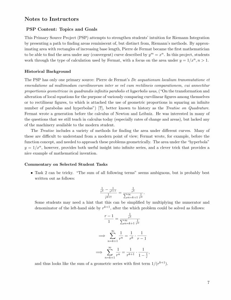
Commentary on Selected Student Tasks

• Task 2 can be tricky. “The sum of all following terms” seems ambiguous, but is probably best

written out as follows:

1rk− 1

rk+1

1rk+1

=1rk∑∞

n=k+11rn.

Some students may need a hint that this can be simplified by multiplying the numerator and

denominator of the left-hand side by rk+1, after the which problem could be solved as follows:

r − 1

1=

1rk∑∞

n=k+11rn

=⇒∞∑

n=k+1

1

rn=

1

rk· 1

r − 1

=⇒∞∑

n=k+1

1

rn=

1

rk+1· 1

1− 1r

,

and thus looks like the sum of a geometric series with first term 1/(rk+1).

7

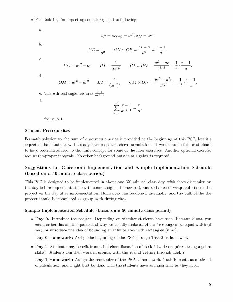
• For Task 10, I’m expecting something like the following:

a.

xH = ar, xO = ar2, xM = ar3.

b.

GE =1

a2GH ×GE =

ar − aa2

=r − 1

a.

c.

HO = ar2 − ar HI =1

(ar)2HI ×HO =

ar2 − ara2r2

=1

r· r − 1

a.

d.

OM = ar3 − ar2 HI =1

(ar2)2OM ×ON =

ar3 − a2ra2r4

=1

r2· r − 1

a.

e. The nth rectangle has area r−1arn−1 .

f.∞∑n=1

r − 1

arn−1=r

a,

for |r| > 1.

Student Prerequisites

Fermat’s solution to the sum of a geometric series is provided at the beginning of this PSP, but it’s

expected that students will already have seen a modern formulation. It would be useful for students

to have been introduced to the limit concept for some of the later exercises. Another optional exercise

requires improper integrals. No other background outside of algebra is required.

Suggestions for Classroom Implementation and Sample Implementation Schedule

(based on a 50-minute class period)

This PSP is designed to be implemented in about one (50-minute) class day, with short discussion on

the day before implementation (with some assigned homework), and a chance to wrap and discuss the

project on the day after implementation. Homework can be done individually, and the bulk of the the

project should be completed as group work during class.

Sample Implementation Schedule (based on a 50-minute class period)

• Day 0. Introduce the project. Depending on whether students have seen Riemann Sums, you

could either discuss the question of why we usually make all of our “rectangles” of equal width (if

yes), or introduce the idea of bounding an infinite area with rectangles (if no).

Day 0 Homework: Assign the beginning of the PSP through Task 3 as homework.

• Day 1. Students may benefit from a full-class discussion of Task 2 (which requires strong algebra

skills). Students can then work in groups, with the goal of getting through Task 7.

Day 1 Homework: Assign the remainder of the PSP as homework. Task 10 contains a fair bit

of calculation, and might best be done with the students have as much time as they need.

8

Day 2: Discuss results – possibly ask students to present their solutions to Task 10. This would

be an especially good time to discuss the idea that we can bound the area of f(x) = 1/x2 to the

right of x = a by r/a2 for any |r| > 1, and to think about what this means in the limiting case as

r → 1.

The LATEX source file for this mini-PSP is available from the author by request at

dominic.klyve@cwu.edu.

Connections to other Primary Source Projects

This is one of three PSPs primarily designed for a first Calculus class in the (growing) TRIUMPHS

collection. Others are:

• How to Calculate π: Machin’s Inverse Tangents, by Dominic Klyve, and

• The Derivatives of the Sine and Cosine Functions, by Dominic Klyve

These projects and others can be found at the TRIUMPHS website at https://blogs.ursinus.edu/triumphs/.

Recommendations for Further Reading

Without a doubt, the most thorough study of Fermat’s work is Michael Sean Mahoney’s The Mathemat-

ical Career of Pierre de Fermat (1601–1665) ([?]). His discussion of Fermat’s “Treatise on Quadrature”

begins on page 243 of his book. The curious reader will find a deeper discussion of his work, including

an important topic excluded from the PSP: that of adequality. The term seems to mean something

like “two things are equal in their limits”, but the details are vexingly complex to modern readers,

and contribute little to the understanding of area. After wrestling with how to introduce the idea to

students for more time than I would like to admit, I removed these sections entirely.

For a discussion of how Fermat’s work can be used in the classroom using modern notation, see

Amy Shell-Gellasch. Integration a la Fermat, in Amy Shell-Gellasch and Dick Jardine, eds., Mathe-

matical Time Capsules: Historical Modules for the Mathematics Classroom, number 77, 111–116,

MAA (2011).

The earliest discussion I could find in print of Fermat’s integration techniques is

Carl B. Boyer. Fermat’s integration of xn. National Mathematics Magazine, 20(1):29–32, 1945,

which should be read by anyone looking to understand the history of our understanding of Fermat’s

work.

Acknowledgments

The development of this student project has been partially supported by the Transforming Instruction in

Undergraduate Mathematics via Primary Historical Sources (TRIUMPHS) Program with funding from

the National Science Foundation’s Improving Undergraduate STEM Education Program under grant

number 1524098. Any opinions, findings, and conclusions or recommendations expressed in this project

9

are those of the author and do not necessarily represent the views of the National Science Foundation.

For more information about TRIUMPHS, visit http://webpages.ursinus.edu/nscoville/TRIUMPHS.

html.

This work is licensed under a Creative Commons Attribution-ShareAlike 4.0

International License. It allows re-distribution and re-use of a licensed work

on the conditions that the creator is appropriately credited and that any

derivative work is made available under “the same, similar or a compatible

license”.

10