Comparison of the generalized Riemann solver and the gas ...

Journal of Computational Physics 230 (2011) 5080–5099

Contents lists available at ScienceDirect

Journal of Computational Physics

journal homepage: www.elsevier .com/locate / jcp

Comparison of the generalized Riemann solver and the gas-kineticscheme for inviscid compressible flow simulations

Jiequan Li a, Qibing Li b, Kun Xu c,⇑a School of Mathematical Sciences, Beijing Normal University, 100875, Chinab Department of Engineering Mechanics, Tsinghua University, 100084, Chinac Department of Mathematics, Hong Kong University of Science and Technology, Kowloon, Hong Kong

a r t i c l e i n f o

Article history:Received 3 November 2010Received in revised form 10 February 2011Accepted 15 March 2011Available online 8 April 2011

Keywords:Generalized Riemann problemGas kinetic schemeInviscid Euler equationsNon-equilibrium flows

0021-9991/$ - see front matter � 2011 Elsevier Incdoi:10.1016/j.jcp.2011.03.028

⇑ Corresponding author. Tel.: +852 2358 7440; faE-mail addresses: [email protected] (J. Li), lqb

a b s t r a c t

The generalized Riemann problem (GRP) scheme for the Euler equations and gas-kineticscheme (GKS) for the Boltzmann equation are two high resolution shock capturingschemes for fluid simulations. The difference is that one is based on the characteristicsof the inviscid Euler equations and their wave interactions, and the other is based onthe particle transport and collisions. The similarity between them is that both methodscan use identical MUSCL-type initial reconstructions around a cell interface, and the spa-tial slopes on both sides of a cell interface involve in the gas evolution process and theconstruction of a time-dependent flux function. Although both methods have beenapplied successfully to the inviscid compressible flow computations, their performanceshave never been compared. Since both methods use the same initial reconstruction,any difference is solely coming from different underlying mechanism in their flux evalu-ation. Therefore, such a comparison is important to help us to understand the correspon-dence between physical modeling and numerical performances. Since GRP is so faithfullysolving the inviscid Euler equations, the comparison can be also used to show the validityof solving the Euler equations itself. The numerical comparison shows that the GRP exhib-its a slightly better computational efficiency, and has comparable accuracy with GKS forthe Euler solutions in 1D case, but the GKS is more robust than GRP. For the 2D high Machnumber flow simulations, the GKS is absent from the shock instability and converges tothe steady state solutions faster than the GRP. The GRP has carbuncle phenomena, likesa cloud hanging over exact Riemann solvers. The GRP and GKS use different physical pro-cesses to describe the flow motion starting from a discontinuity. One is based on theassumption of equilibrium state with infinite number of particle collisions, and the otherstarts from the non-equilibrium free transport process to evolve into an equilibrium onethrough particle collisions. The different mechanism in the flux evaluation deviates theirnumerical performance. Through this study, we may conclude scientifically that it mayNOT be valid to use the Euler equations as governing equations to construct numericalfluxes in a discretized space with limited cell resolution. To adapt the Navier–Stokes(NS) equations is NOT valid either because the NS equations describe the flow behavioron the hydrodynamic scale and have no any corresponding physics starting from a discon-tinuity. This fact alludes to the consistency of the Euler and Navier–Stokes equations withthe continuum assumption and the necessity of a direct modeling of the physical processin the discretized space in the construction of numerical scheme when modeling veryhigh Mach number flows. The development of numerical algorithm is similar to the

. All rights reserved.

x: +852 2358 [email protected] (Q. Li), [email protected] (K. Xu).

http://dx.doi.org/10.1016/j.jcp.2011.03.028

mailto:[email protected]



http://dx.doi.org/10.1016/j.jcp.2011.03.028

http://www.sciencedirect.com/science/journal/00219991

http://www.elsevier.com/locate/jcp

J. Li et al. / Journal of Computational Physics 230 (2011) 5080–5099 5081

modeling process in deriving the governing equations, but the control volume here cannotbe shrunk to zero.

� 2011 Elsevier Inc. All rights reserved.

1. Introduction

The modern computational fluid dynamics (CFD) method for compressible flow is based on the Riemann problem frompiecewise constant states [14]. The necessity to use discontinuous initial condition is due to the limited cell resolution torepresent physical flow structure. Due to the preparation of discontinuous initial data through the so-called nonlinear lim-iter, the numerical dissipation is implicitly added in the shock capturing schemes. In the past decades, the shock capturingCFD methods based on the exact or approximate Riemann problems are extremely successful in the engineering applicationsand the scientific study of compressible flows. In order to further increase the accuracy, generalized Riemann solvers underpiecewise linear discontinuous initial data were developed. The generalized Riemann problem (GRP) was proposed for com-pressible flows based on the Lagrangian formulation first [2,4], and a direct Eulerian version was developed in [6,5] using theconcept of Riemann invariants. Theoretically, in the GRP, a close coupling between the spatial and temporal evolution isrecovered through the analysis of detailed wave interactions. The GRP is more precise and accurate than any other approx-imate Riemann solvers. It is the most accurate description of the Euler solutions under its corresponding initial condition.The schemes based on the GRP have been applied successfully to many engineering problems [1,3,12,13,18].

On the other hand, based on the gas-kinetic theory, the Euler and Navier–Stokes equations can be derived from theBoltzmann equation using the Chapman–Enskog expansion [9]. In a gas-kinetic representation, all flow variables aremoments of a single particle distribution function. In the past years, a gas-kinetic scheme (GKS) based on the BGK model[7] has been developed for the compressible flow simulation under linear polynomials for the mass, momentum, and energydistributions separated by discontinuities at the origin [32,23]. The GKS has been successfully applied in many engineeringapplications, especially for the hypersonic viscous and heat conducting flows [33,20,21].

In this paper, we are going to compare the performance of GRP and GKS in many 1D and 2D flow computations, especially tothe test cases on which many other schemes may have difficulties, e.g. the large density ratio problem [27], highly expansionwave, and the blunt body problem. Since GRP and GKS use the identical initial reconstruction and follow explicitly their timeevolution within a time step, any difference between these two methods must come from the dynamic mechanism in their fluxconstruction. The GRP and GKS are following different physical processes in the description of flow motion starting from a dis-continuity. Their comparison definitely gives us useful information about the correspondence between the physical modelingand numerical performance. This is also the main reason why we do not use other Riemann solvers. For many other Riemannsolvers, the problem is that either the real governing equations are unknown, or they are constructed in an ad hoc ways. TheGRP truthfully follows the Euler solution and it has the most accurate Euler flux under the corresponding initial condition.

Based on the comparison and analysis in this paper, we come into the following conclusion. For algorithm development,the direct physical modeling of the gas evolution process in a discretized space is more fundamental and important thanadapting any presumed governing equation from the start point. The Euler equations can be only used to describe the equi-librium flow, which is incapable to describe the non-equilibrium effects inside a numerical strong shock layer. Due to the cellresolution, the non-equilibrium flow region has been numerically enlarged. The physical process in the GRP is inadequate indescribing the flow behavior in this region. As a result, the carbuncle phenomenon is intrinsically rooted in the exact Rie-mann solver. Since GRP is so accurate in solving the Euler equations, through this research we would like to raise the ques-tions about the validity of directly using a governing equation which has infinite wave resolution to a space with limited cellsize and time step. Due to the inclusion of both kinetic and hydrodynamic scale physics in the kinetic formulation, the GKSprovides a more reliable gas evolution model than GRP to describe flow starting from a discontinuity. We hope that throughthis study and any other following up research, the CFD will evolve from an art-based to a science-based research subject.

2. Generalized Riemann problem and gas-kinetic schemes

In this paper we will focus on the comparison of numerical results for the compressible Euler equations,

ut þ FðuÞx þ GðuÞy ¼ 0;

u ¼ ðq;qU;qV ;qEÞ>;FðuÞ ¼ ðqU;qU2 þ p;qUV ;UðqEþ pÞÞ>;GðuÞ ¼ ðqV ;qUV ;qV2 þ p;VðqEþ pÞÞ>;

ð1Þ

where q; ðqU;qVÞ and qE are conserved variables of the density, the momentum and the total energy with E ¼ U2þV2

2 þ e; e theinternal energy, p is the pressure and p ¼ ðc� 1Þqe for polytropic gases. Then following the finite volume formulation, wewrite (1) as

unþ1j ¼ un

j �1jXjj

Xm

i¼1

Z tnþ1

tnFijdt; ð2Þ

5082 J. Li et al. / Journal of Computational Physics 230 (2011) 5080–5099

where Xi is the control volume with sides Cij; j ¼ 1; . . . ;m (m ¼ 4 in this paper), n ¼ ðnj1;nj2Þ is the outer normal of Cij, andthe numerical flux Fij is

Fij ¼Z

Cij

ðF;GÞðuÞ � ðni1; ni2ÞdC; ð3Þ

where unj is the usual average of uðx; tnÞ over Xj. In one-dimensional case, Xj ¼ ðxj�1

2; xjþ1

2Þ and the center xj ¼ xj�1

2þ xjþ1

2

� �=2.

The GRP and GKS both provide a respective time-dependent flux function from a piecewise linear discontinuous initial data.In this section, we are going to first present the reconstruction used in the present paper.

As expressed in (2), at the beginning of each time step t ¼ tn only cell averaged mass, momentum and energy densities aregiven. As far as a high-resolution scheme is concerned, interpolation techniques are used to construct the subcell structure.Simple polynomials usually generate spurious oscillations if large gradients exist in the data. The most successful interpo-lation techniques known so far are those based on the concepts of limiters [8,29], and these interpolation rules can beapplied to the conservative, characteristic or primitive flow variables. In this paper, the reconstruction is solely applied tothe conservative variables. The limiter used is the van Leer limiter. With the cell averaged component of conservativevariables wj, and their differences between neighboring cells sþ ¼ ðwjþ1 �wjÞ=Dx and s� ¼ ðwj �wj�1Þ=Dx, the slope of win cell j is constructed as

Lðsþ; s�Þ ¼ Sðsþ; s�Þjsþjjs�jjsþj þ js�j

;

where Sðsþ; s�Þ ¼ signðsþÞ þ signðs�Þ. After reconstruction, the flow variable w is distributed linearly in cell j,

�wjðxÞ ¼ wj þ Lðsþ; s�Þðx� xjÞ; xj�12< x < xjþ1

2:

The interpolated flow distribution around a cell interface is shown in Fig. 1. Both the GRP and GKS are based on the aboveinitial data to evaluate a time-dependent local solution.

2.1. The Generalized Riemann problem for the inviscid Euler equations

The generalized Riemann problem (GRP) scheme starts directly from (1). Denote by Pij the middle point of Cij andFij ¼ ðF;GÞ � ðni1;ni2Þ. Then the GRP uses the middle point value to directly approximate the flux F

nþ12

ij , within the accuracyof second order,

Fnþ1

2ij � Fij u Pij; nþ 1

2

� �Dt

� �� : ð4Þ

One of main issues is how to calculate the mid-point value uðPij; nþ 12

� �DtÞ using as much characteristics of (1) as possible.

Here we use the Taylor series expansion,

uðPij; nþ 12

� �DtÞ ¼ uðPij; tn þ 0Þ þ Dt

2@u@tðPij; tn þ 0Þ þ OðDt2Þ: ð5Þ

Fix the cell interface Cij and denote by

u� ¼ uðPij; tn þ 0Þ; @u@t

� ��¼ @u@tðPij; tn þ 0Þ: ð6Þ

Fig. 1. The reconstructed initial conservative variables around a cell interface.

Fig. 2. A typical wave pattern for the GRP. The initial data u0ðxÞ ¼ u‘ þ xu0‘ for x < 0 and u0ðxÞ ¼ ur þ xu0r for x > 0.


The first instantaneous value u� is obtained with the standard Riemann solver [4,28]. The main contribution of the GRPscheme is how to obtain the instantaneous value of time derivative ð@u=@tÞ� analytically, which boils down to solving theassociated generalized Riemann problem along each cell interface Cij. For this purpose, we shift ðPij; tnÞ to the coordinate ori-gin ð0;0;0Þ and make Cij coincide with the y-axis. Then we define the quasi-one-dimensional (planar) generalized Riemannproblem for

ut þ FðuÞx ¼ 0; ð7Þ

subject to the initial data

uðx; y;0Þ ¼u‘ þ xu0x‘ þ yu0y‘; x < 0;ur þ xu0xr þ yu0yr; x > 0;

(ð8Þ

where u‘;u0x‘;u0y‘;ur ;u0xr ;u

0yr are constant vectors. In particular, as u0y‘ and u0yr vanishes, Eq. (8) becomes planar one-dimen-

sional flows. The conventional GRP solver uses the planar one-dimensional Euler equations (7) for simplicity and efficiency.Then we assume the wave configuration from the y-axis as shown in Fig. 2, in which a curved rarefaction wave moves to theleft, a shock to the right and the t-axis is located in the intermediate region. Other cases can be treated similarly. We remindthat as the initial data is uniform, i.e., piecewise constant, the rarefaction wave in Fig. 2 becomes isentropic, referred as acentered rarefaction wave (CRW). As the initial data is not uniform the instantaneous value of time derivative ð@u=@tÞ�can be solved in the following proposition.

Proposition 1. Let ð@u=@tÞ� be the instantaneous time derivative of u evaluated at the origin. Then ð@U=@tÞ� and ð@p=@tÞ� aredetermined by solving a pair of linear equations

a‘@U@t

� ��þ b‘

@p@t

� ��¼ d‘;

ar@U@t

� ��þ br

@p@t

� ��¼ dr ;

ð9Þ

where the coefficients a‘; b‘ and d‘ depends on u�;u‘ and u0‘; and ar ; br and dr depends on u�;ur and u0r . The instantaneous timederivative of the density q is given by the state equation p ¼ pðq; SÞ; S is the entropy,

dp ¼ c2dqþ @p@S

dS: ð10Þ

The velocity component V satisfies

Vt þ UVx ¼ 0: ð11Þ

It resembles the entropy variable S (cf. (17) below) and can be treated similarly.

All these coefficients can be obtained explicitly as presented in [6]. It turns out that the coding process is almost the same asa 2� 2 linear system that we will show below. In the derivation of this proposition, the fundamental idea is to extract sin-gularities (discontinuities) from the complex wave patterns:

Wave patterns ¼ a singular partþ a regular part: ð12Þ


The GRP scheme expresses and manipulates the regular part using Riemann invariants and leave the singular part aside. Thismanipulation is indispensable. Below is a heuristic example of a linear toy system in order to explain (12) clearly,

ut þ avx ¼ 0;v t þ aux ¼ 0;

ð13Þ

where a > 0 is a constant. In consistent with the notations in (8), u ¼ ðu;vÞ> here. In order to develop the second order MUS-CL-type (upwind) scheme for (13), the piecewise linear data is given

uðx;0Þ ¼u‘ þ xu0‘; x < 0;ur þ xu0r; x > 0

�ð14Þ

and we need to know the intermediate value uð0; tÞ along the t-axis. Note that the initial data contains a discontinuity at theorigin, causing nontrivial singularities (discontinuities) that propagate along characteristics x ¼ �at, which implies that boththe variables u and v are discontinuous across x ¼ �at. In order to cope with this difficulty, it is necessary to extract out thesingularities in some sense. For this purpose, we make the following manipulation for (13)

ðuþ vÞt þ aðuþ vÞx ¼ 0;ðu� vÞt � aðu� vÞx ¼ 0:

ð15Þ

Then the assembled quantity uþ v is continuous in the region fðx; tÞ; x < at; t > 0g although both u and v are discontinuousacross x ¼ �at. The same is true for u� v in the region fðx; tÞ; x > �at; t > 0g. Thus we use uþ v and u� v as new dependentvariables to easily obtain

u� þ v� ¼ u‘ þ v ‘; u� � v� ¼ ur � v r;

@u@t

� ��þ @v

@t

� ��¼ �a u0‘ þ v 0‘

� �;

@u@t

� �� @v

@t

� ��¼ a u0r � v 0‘

� �:

ð16Þ

Then, in turn, we obtain u� and ð@u=@tÞ� by solving the pairs of linear equations (16).The crucial point in the above process is that the assembled quantity uþ v (resp. u� v) is continuous across the discon-

tinuity xþ at ¼ 0 (resp. x� at ¼ 0). It has several implications:

(1) The assembled quantities uþ v and u� v , corresponding to the Riemann invariants for (1), are used to achieve theclaim (12). More precisely, take a look at the characteristic x ¼ �at, across which, as mentioned above, both u andv are discontinuous. However, uþ v is regular there and the singularity along x ¼ �at has been removed solely ontou� v . Then we can manipulate uþ v as a scalar variable for a single linear advection equation.

(2) In smooth regions, the Lax–Wendroff approach can be used to define the instantaneous time derivatives of (proper)assembled variables, which are replaced by the spatial derivatives.

(3) The resulting pair of linear equations are then solved to obtain the instantaneous time derivatives of primitive vari-ables finally.

It seems that this is the only reasonable way to extend a scalar case to the system (13) in order to construct the numerical fluxwith the least numerical dissipation under the second order MUSCL-type initial condition. The GRP methodology for (1) usesalmost the same idea: look for Riemann invariants, extract singularities, and derive a pair of linear equations (9), particularlyin the resolution of rarefaction waves. Since the entropy variable is necessarily taken as one of Riemann invariants and exactlycomputed, the rarefaction wave can be well resolved so that the resulting scheme is able to capture both (even very strong)rarefaction and shocks waves. Let us illuminate this in some detail. We fix the case of the left-moving rarefaction wave asso-ciated with the characteristic field U � c; c is the sound speed, as shown in Fig. 2. The primitive variables ðq;U; pÞ (or the con-servative variables ðq;qU;qEÞ) are singular through the rarefaction wave, particularly around the origin. Use the Riemanninvariants wðq;U; pÞ ¼ U þ 2c

c�1 and S (for polytropic gases, and similarly for general gases) to write (1) in terms of w and S as

wt þ ðU þ cÞwx ¼ TSx;

St þ USx ¼ 0;ð17Þ

where T is the temperature. Since w keeps invariant across the centered isentropic rarefaction wave (CRW) in the associatedRiemann problem, it behaves exactly like uþ v for (13) and be smooth through the entire curved rarefaction wave in the gen-eralized Riemann problem. Therefore, we can use the regularity property of w across the rarefaction wave so that usual cal-culus manipulations can be made. The singularity of the solution is removed onto another variable / ¼ U � 2c

c�1 that satisfies

/t þ ðU � cÞ/x ¼ TSx: ð18Þ

Note that / is also a Riemann invariant but associated with another characteristic field U þ c. We resolve (17) to obtain thefirst equation of (9).

The second equation of (9) can obtained through tracing the right-going shock trajectory, following van Leer’s idea [29].The source terms in (17) and (18) reflect the variation of entropy as the initial state is not uniform. This variation is well

captured in the GRP scheme, and then the variable w is resolved subsequently in an analytical way, using the Lax–Wendroff


approach. Due to the regularity of w and S and their analytical resolution, it is expected that the rarefaction wave can be cap-tured very accurately using the GRP scheme, and it is indeed. The detail can be found in [6,5].

2.2. The gas-kinetic scheme

In this section, a directional splitting method to solve the 2D BGK equation will be presented. The BGK model in the x-direction can be written as [9]

ft þ ufx ¼g � f

s; ð19Þ

where f is the gas distribution function, g is the equilibrium state approached by f, and s is the particle collision time. Both fand g are functions of space x, time t, particle velocities ðu;vÞ, and internal variable n. The particle collision time s is related tothe viscosity and heat conduction coefficients. The equilibrium state is a Maxwellian distribution,

g ¼ qkp

� �Kþ22

e�kððu�UÞ2þðv�VÞ2þn2Þ;

where q is the density, U and V are the macroscopic velocities in the x and y directions, as in (1), and k ¼ m=2kT , where m isthe molecular mass, k is the Boltzmann constant, and T is the temperature. Within the equilibrium state g, the ideal gas equa-tion of state is implicitly imposed because the pressure p evaluated from g will be equal to p ¼ q=2k ¼ qRT . For a 2D flowwith explicit account of U and V velocities, the random particle motion in the z direction is included into the internal variablen, and the total number of degrees of freedom K in n is equal to ð5� 3cÞ=ðc� 1Þ þ 1. For example, for a diatomic molecular inthe 2D simulation, K will be equal to 3, which accounts for the molecule random motion in the z-direction and two rotationaldegrees of freedom. In the equilibrium state, the internal variable n2 is equal to n2 ¼ n2

1 þ n22 þ � � � þ n2

K . The relation betweenmass q, momentum ðn ¼ qU;m ¼ qVÞ, and energy qE densities with the distribution function f is

qn

m

qE

0BBB@

1CCCA ¼

ZwafdN; a ¼ 1;2;3;4; ð20Þ

where wa is the component of the vector of moments

w ¼ ðw1;w2;w3;w4Þ> ¼ 1; u;v ;1

2ðu2 þ v2 þ n2Þ

� �>
and dN ¼ dudvdn is the volume element in the phase space with dn ¼ dn1dn2 . . . dnK . Since mass, momentum and energy areconserved during particle collisions, f and g satisfy the conservation constraint, Z
ðg � f ÞwadN ¼ 0; a ¼ 1;2;3;4; ð21Þ

at any point in space and time. For a local equilibrium state with f ¼ g, the Euler equations can be obtained by taking themoments of wa to Eq. (19). This yields
Z
waðgt þ ugxÞdN ¼ 0; a ¼ 1;2;3;4

and the corresponding Euler equations in the x-direction will be the same as Eq. (1). The general solution f of the BGK model(19) at a cell interface xjþ1=2 and time t is

f ðxjþ1=2; t;u;v ; nÞ ¼1s

Z t

0gðx0; t0;u; v; nÞe�ðt�t0 Þ=sdt0 þ e�t=sf0ðxjþ1=2 � utÞ; ð22Þ

where x0 ¼ xjþ1=2 � uðt � t0Þ is the particle trajectory and f0 is the initial gas distribution function f at the beginning of eachtime step ðt ¼ 0Þ. Two unknowns g and f0 must be specified in Eq. (22) in order to obtain the solution f. In order to simplifythe notation, xjþ1=2 ¼ 0 will be used in the following text. Based on the MUSCL-type reconstruction for the macroscopic vari-ables at a cell interface, the initial gas distribution function f0 has the corresponding form,

f0 ¼gl½1þ alx� sðaluþ AlÞ�; x 6 0;gr½1þ arx� sðaruþ ArÞ�; x P 0;

(ð23Þ

where the terms being proportional to s are the nonequilibrium states obtained from the Chapman–Enskog expansion of theBGK model. The parameters of ðal;Al

; ar;ArÞ are related to the Taylor expansion of a Maxwellian. The nonequilibrium partshave no direct contribution to the conservative variables, i.e.,
Z
ðaluþ AlÞwgldN ¼ 0;Zðaruþ ArÞwgrdN ¼ 0:

ð24Þ


After having f0, the equilibrium state g around ðx ¼ 0; t ¼ 0Þ is assumed to have two slopes,

g ¼ g0½1þ ð1�H½x�Þ�alxþH½x��arxþ At�; ð25Þ

where H½x� is the Heaviside function defined as

H½x� ¼0; x < 0;1; x P 0:

�

Here g0 is a local Maxwellian distribution function located at x ¼ 0. Even though, g is continuous at x ¼ 0, but it has differentslopes at x < 0 and x > 0. In both f0 and g; al;Al

; ar ;Ar; �al; �ar , and A are related to the derivatives of Maxwellians in space and

time. Detailed formulation can be found in [32].In the reconstruction stage, we have obtained the distributions �qjðxÞ; �mjðxÞ; �njðxÞ, and qjEjðxÞinside each cell

xj�1=2 6 x 6 xjþ1=2. At the cell interface xjþ1=2, the left and right macroscopic states are

ujðxjþ1=2Þ ¼

�qjðxjþ1=2Þ�mjðxjþ1=2Þ�njðxjþ1=2Þ�qEjðxjþ1=2Þ

0BBB@

1CCCA; ujþ1ðxjþ1=2Þ ¼

�qjþ1ðxjþ1=2Þ�mjþ1ðxjþ1=2Þ�njþ1ðxjþ1=2Þ

�qEjþ1ðxjþ1=2Þ

0BBB@

1CCCA:

x

p

0 20 40 60 80 1000

100

200

300

400BGK (N=800)BGK (N=3200)GRP (N=800)

x

u

0 20 40 60 80 1000

2

4

6

8

10

12

14

BGK (N=800)BGK (N=3200)GRP (N=800)

x

e

0 20 40 60 80 1000

200

400

600

800

1000

1200

1400

BGK (N=800)BGK (N=3200)GRP (N=800)

Fig. 3. Woodward–Colella blast wave problem. (a) pressure, (b) velocity, (c) internal energy.


By using the relation between the gas distribution function f and the macroscopic variables (Eq. (20)), at xjþ1=2 we get
ZglwdN ¼ ujðxjþ1=2Þ;
ZglalwdN ¼ ujðxjþ1=2Þ � ujðxjÞ

Dx�; ð26ÞZ

grwdN ¼ ujþ1ðxjþ1=2Þ;Z

grarwdN ¼ ujþ1ðxjþ1Þ � ujþ1ðxjþ1=2ÞDxþ

; ð27Þ

where Dx� ¼ xjþ1=2 � xj and Dxþ ¼ xjþ1 � xjþ1=2. Based on the above equations, all parameters in the initial distribution func-tion f0 can be fully determined.

After determining f0, the corresponding values of q0;U0;V0 and k0 in g0 of Eq. (25), i.e.,

g0 ¼ q0k0

p

� �Kþ22

e�k0ððu�U0Þ2þðv�V0Þ2þn2Þ;

can be determined as follows. Taking the limit t ! 0 in Eq. (22) and substituting its solution into Eq. (21), the conservationconstraint at ðx ¼ xjþ1=2; t ¼ 0Þ gives

Zg0wdN ¼ u0 ¼

Zu>0

ZglwdNþ

Zu<0

ZgrwdN; ð28Þ

where u0 ¼ ðq0;m0;n0;q0E0ÞT are the macroscopic conservative flow variables located at the cell interface at time t ¼ 0.

x

p

0 20 40 60 80 1000

0.1

0.2

0.3

0.4BGKGRPExact

x

u

0 20 40 60 80 100-3

-2

-1

0

1

2

3

BGKGRPExact

x

E

0 20 40 60 80 1000

1

2

3

BGKGRPExact

Fig. 4. Sjogreen’s low density problem. (a) pressure, (b) velocity, (c) energy.


Then, �al and �ar of g in Eq. (25) can be obtained through the relation of

ujþ1ðxjþ1Þ � u0

q0Dxþ¼ M0

ab

�ar1

�ar2

�ar3

�ar4

0BBB@

1CCCA ¼ M0

ab�ar

b ð29Þ

and

u0 � ujðxjÞq0Dx�

¼ M0ab

�al1

�al2

�al3

�al4

0BBB@

1CCCA ¼ M0

ab�al

b; ð30Þ

where the matrix M0ab ¼

Rg0wawbdN=q0 is known.

Up to this point, we have determined all parameters in the initial gas distribution function f0 and the equilibrium state gat the beginning of each time step t ¼ 0. After substituting Eqs. (23) and (25) into Eq. (22), the gas distribution function f at acell interface can be expressed as

f ðxjþ1=2; t;u;v ; nÞ ¼ ð1� e�t=sÞg0 þ ðsð�1þ e�t=sÞ þ te�t=sÞð�alH½u� þ �arð1�H½u�ÞÞug0 þ sðt=s� 1þ e�t=sÞAg0

þ e�t=sðð1� uðt þ sÞalÞH½u�gl þ ð1� uðt þ sÞarÞð1�H½u�ÞgrÞþ e�t=sð�sAlH½u�gl � sArð1�H½u�ÞgrÞ: ð31Þ

x

ρ

0 20 40 60 80 100100

101

102

103

104

BGK (N=100)BGK (N=400)GRP (N=100)GRP (N=400)Exact

x

p

0 20 40 60 80 100100

101

102

103

104


x

u

0 20 40 60 80 1000

1

2

3

4BGK (N=100)BGK (N=400)GRP (N=100)GRP (N=400)Exact

x

e

0 20 40 60 80 1000

2

4

6

8

10

12BGK (N=100)BGK (N=400)GRP (N=100)GRP (N=400)Exact

Fig. 5. Large density ratio problem. (a) density, (b) pressure, (c) velocity, (d) internal energy.


The only unknown left in the above expression is A. Since both f (Eq. (31)) and g (Eq. (25)) contain A, the integration of theconservation constraint Eq. (21) at xjþ1=2 over the whole time step Dt gives
Z Dt
0

Zðg � f ÞwdtdN ¼ 0:

The evaluation of A is about to get time variation of macroscopic variables at a cell interface, which is similar to the GRP inthe evaluations of ð@U=@tÞ� and ð@p=@tÞ�.

Finally, the time-dependent numerical fluxes in the x-direction across the cell interface can be computed as

Fq

Fm

Fn

FqE

0BBB@

1CCCA

jþ1=2

¼Z

u

1uv

12 ðu2 þ v2 þ n2Þ

0BBB@

1CCCAf ðxjþ1=2; t;u;v ; nÞdN; ð32Þ

where f ðxjþ1=2; t; u;v ; nÞ is given in Eq. (31). By integrating the above equation to the whole time step, we can get the totalmass, momentum and energy transport. For the Euler solutions, theoretically the particle collision time s should approachto zero in order to keep the equilibrium state everywhere. As a result, the only terms left in (31) will be these related to theequilibrium one, which has the similar mechanism as the Riemann solver. However, the molecules in any flow system havelimited mean free path and particle collision time. Starting from a discontinuity, the flow behavior will depend on the ratiobetween the time passed and particle collision time. The formulation (31) describes such a relaxation process from the mol-

x

ρ

0 20 40 60 80 100100

101

102

103

104

BGK (N=100)BGK (N=400)Exact

x

p

0 20 40 60 80 100100

101

102

103

104

BGK (N=100)BGK (N=400)Exact

x

u

0 20 40 60 80 1000

1

2

3

4BGK (N=100)BGK (N=400)Exact

x

e

0 20 40 60 80 1000

2

4

6

8

10

12BGK (N=100)BGK (N=400)Exact

Fig. 6. Large density ratio problem. (a) density, (b) pressure, (c) velocity, (d) internal energy.


ecule free transport to the equilibrium state formation. The Euler solution is achieved only in the limiting case of t=s!1.Theoretically, the particle collision time s is equal to the mean free path over particle speed. In a discretized space, due to thelimited cell resolution we will not have infinite flow structure resolution. Therefore, the particle mean free path needs to takeaccount of the cell resolution as well. For the Euler solution, which has no any characteristic scale, the mean free pathcan be assumed to be proportional to the cell size. The collision time used in all test cases in this paper have the followingform,

s ¼ Dxffiffiffiffiffik0

pðaþ bjpl � pr j=ðpl þ prÞÞ ð33Þ

with a ¼ 0:05 and b ¼ 1:0, where k0 is given in the equilibrium state g0, and pl and pr are the pressure jump at the cell inter-face in the initial reconstructed data. The consideration for the above formulation is the following. As mesh size goes to zero,s will go to zero as well, and the GKS converges to the Euler solutions. In comparison with flux vector splitting scheme, withthe above definition of particle collision time there will have tens of particle collisions within each time step. In other words,the numerical dissipation introduced in the above formulation is much less than that in the flux vector splitting method.

In the continuum flow regime, the initial free transport part in the gas distribution function (31) disappears. The evolutionof continuous flow will converge to the equilibrium state quickly. However, in the dissipative shock region, the numericalparticle mean free path is much enlarged to capture the non-equilibrium effect, such as the real physical process inside ashock layer. This is equivalent to enlarging the physical shock thickness to the cell size scale, and the GKS provides theparticle transport and collision mechanism here.

x

ρ

80 82 84 86 88 90

1

2

3

4


x

p

80 82 84 86 88 900

0.2

0.4

0.6

0.8

1

1.2

1.4


x

u

80 82 84 86 88 90

-1.2

-1

-0.8

-0.6

-0.4


x

e

80 82 84 86 88 90

0

0.2

0.4

0.6


Fig. 7. Slowly moving shock problem. (a) density, (b) pressure, (c) velocity, (d) internal energy.


3. Details of the test cases

In this section we will present quite full comparison of numerical results by the GRP and GKS schemes. These examplesare all very challenging, ranging from several one-dimensional blast wave problem to the high speed flow impinging on acylinder. Unless otherwise stated, the van Leer limiter is adopted and the CFL number is set to be 0.5. Since GRP and GKSuse the identical van Leer limiter for the conservative flow variables reconstruction, any difference in the simulation resultsis due to the flux function, i.e., the mechanism of gas evolution models around a cell interface. Since GRP is truthfully solvingthe Euler equations and the GKS is following the kinetic equation, the comparison distinguishes the effects of different phys-ical processes on the simulation results.

3.1. Problems in one-dimensional space

3.1.1. Woodward–Colella blast wave problemWe first show the interacting blast wave problem proposed in [30]. The diatomic gas is initially at rest, and the density is

everywhere unit. The pressure is p ¼ 1000 for 0 6 x < 10 and p ¼ 100 for 90 < x 6 100, while it is only p ¼ 0:01 in10 < x < 90. Reflecting boundary conditions are applied at both ends. Numerical results with 800 grid points are shownin Fig. 3 to exhibit the performance of both schemes. This test case clearly demonstrates the capability of both schemesin the capturing of strong shock waves. The GRP presents a little bit sharper solution than the GKS in the internal energydistribution.

Fig. 8. Formation of spiral in the 2D Riemann problem.

Fig. 9. Meshes in cylinder case. (a) 54� 20, (b) 54� 20, (c) 80� 14, (d) 160� 28.


3.1.2. Low density problemThis example was first proposed in [10] for demonstrating the ability of a numerical scheme to preserve the positivity of

density and internal energy. In contrast to the blast wave problem, this test shows strong rarefaction waves. The initial datais given with ðq;U; pÞ ¼ ð1;�2;0:4Þ for 0 6 x < 50 and ðq;U; pÞ ¼ ð1;2;0:4Þ for 50 6 x 6 100. The number of grid points usedhere is 100. Both schemes work well, as shown in Fig. 4. Many approximate Riemann solvers may fail in this test case [10].

3.2. Large density ratio problem

This example was proposed in [27] to test the ability to capture extremely strong rarefaction wave and its influence onthe shock location. In the original paper, it shows that most MUSCL-type schemes have defects in resolving, even withvery fine mesh, the correct wave structures. In this problem, initially the pressure and density ratio between two neigh-boring states are very high. The initial data is ðq;U; pÞ ¼ ð10000;0;10000Þ for 0 6 x < 30 and ðq;U; pÞ ¼ ð1;0;1Þ for

M1.91.71.51.31.10.90.70.50.30.1

M1.91.71.51.31.10.90.70.50.30.1

T

220210200190180170160150140130

T

220210200190180170160150140130

Fig. 10. M ¼ 2 Case with mesh (a). The left column is computed by the GKS and the right by the GRP.


30 6 x 6 100. CFL number is set as 0.32. The results with 100 and 400 points from both GRP and GKS are shown in Fig. 5.For GRP, from 100 to 400 grid points, the shock location converges to the correct position. With 400 grid points, the GRPscheme gives perfect results, which can be comparable to those from very high resolution schemes, i.e., the fifth orderWENO scheme with 10000 grid points [27]. Surprisingly, the GKS presents the same shock front location with 100 and400 grid points. One of the reason is that the GKS solves viscous governing equations, but the exact solution is the inviscidone. In order to clarify the situation, we reduce the particle collision time in Eq. (33) to a ¼ b ¼ 10�4. With the reducing ofdissipation, the GKS results with 100 and 400 grid points are shown in Fig. 6. Again, the GKS keeps almost the same shocklocation for 100 and 400 grid points. Even with 100 grid points, it can capture the solution very well. This clearly dem-onstrates that the GKS converges to the inviscid Euler solution as the particle collision time reduces. In the coarse meshcases, this test clearly shows that the shock speed of GRP is slower than that of GKS. This is probably due to the startingerror in the first few time steps from the initial strong discontinuity. The detail reason needs further investigation.

3.3. Slowly moving shock

This is a test case for strong slowly moving shock with the minmod limiter for both schemes. The initial data is:ðq;U; pÞ ¼ ð4:0;0:3;4=3Þ for 0 6 x < 20; and ðq;U; pÞ ¼ ð1:0;�1:3;10�6Þ for 20 < x 6 100. The polytropic index is taken tobe c ¼ 5=3. This is an almost infinite strong shock in the sense that the density ratio is close to its maximum.

The simulation results from both 100 and 400 grid points are shown in Fig. 7. The shock fronts are captured crisply byboth schemes. In the coarse mesh with 100 grid points, the GKS has a better shock location. As the mesh is refined, bothschemes converge to the exact solution. The GKS generates less magnitude of post-shock oscillation than GRP.

The above several examples are fully recognized as severe test problems and many shock capturing schemes may fail toprovide accurate or even correct results, such as the correct position of shock front in [27]. The GRP and GKS encounter nodifficulties for these cases. One of the reason is that both schemes can compute the entropy accurately. As a result, the rar-efaction wave is resolved perfectly, so is the shock location. Also, through the comparison we can realize that the accuracy ofGKS in obtaining the inviscid Euler solutions even though it targets on the kinetic model.

3.4. Problems in two-dimensions

In comparison with the 1D test cases, two-dimensional simulations are much more interesting and challenging. The GRPis basically 1D gas evolution model. In order to make GKS be consistent with GRP, we adapt the direction splitting GKS herein all simulations. A multi-dimensional GKS scheme has been developed as well [33]. In the 2D case, some classical testproblems such as double Mach reflection have been reported in [15,32] using these two schemes. Here we choose two prob-lems of interaction of (compressible) vortex sheets and the flow impinging on a cylinder. The CFL number is set to be 0.5 and0.7, respectively.

3.4.1. Formation of spiral through the interaction of vortex sheetsThis is a special case of 2D Riemann problems formulated in [34] to simulate the formation of spirals, see also [19,15] for

the solution structure. The initial data is a constant state in each quadrant: ðq;U;V ; pÞ ¼ ð0:5;0:5;�0:5;5Þ forx > 0; y > 0; ðq;U;V ; pÞ ¼ ð1:0;0:5;0:5;5Þ for x < 0; y > 0; ðq;U;V ; pÞ ¼ ð2:0;�0:5;0:5;5Þ for x < 0; y < 0; ðq;U;V ; pÞ ¼ ð1:5;

Time Step

Res_ρ

5000 10000 1500010-10

10-8

10-6

10-4

10-2

100

102BGKGRP

Fig. 11. M ¼ 2 Case with mesh (a). Convergence residue distribution.


�0:5;�0:5;5Þ for x > 0; y < 0. Initially four vortex sheets are supported, respectively, on the x- and y-axes with the same sign,but they have different amounts of measures. They interact immediately after t > 0 to generate a spiral in the center and thestate there closes to the vacuum. We can see the wonderful performance of both schemes from Fig. 8 by the comparison withthose in [26,22,17].

3.4.2. Flow impinging on a cylinderFor the blunt body simulations, we test flows with Mach number 2, 5 and 10. Also, four meshes have been used, which are

shown in Fig. 9. We call them mesh (a), (b), (c) and (d). The difference between mesh (a) and (b) comes from the different sizeof the computational domains to account for the standoff distance of the bow shock. The length–width (circumferential-radial) ratio of Mesh (c) is a little smaller. Mesh (d) is a refined version of mesh (c) with double grid points in both directions.At M ¼ 2 with mesh (a), GRP and GKS can capture the flow structure nicely in front of the cylinder, which are shown inFig. 10 for the Mach number and temperature distributions. The residual for both calculation is shown in Fig. 11. The GKS

M

4.64.23.83.43.02.62.21.81.41.00.60.2

M

4.64.23.83.43.02.62.21.81.41.00.60.2

T740700660620580540500460420380340300260220180140

T740700660620580540500460420380340300260220180140

Fig. 12. M ¼ 5 Case with mesh (b). The left column is computed by the GKS and the right by the GRP.

Time Step

Res_ρ

0 10000 20000 3000010-10

10-8

10-6

10-4

10-2

100

102

104BGKGRP

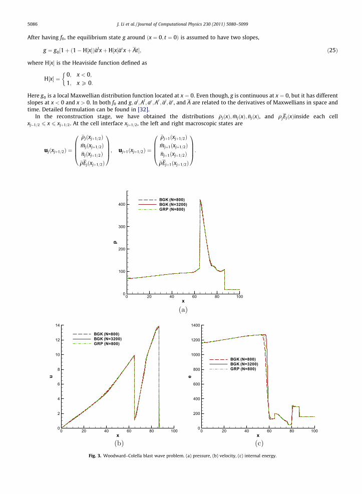
Fig. 13. M ¼ 5 Case with mesh (b). Convergence residue distribution.


converges to machine zero quickly and the convergence of GRP is saturated at 10�4. At M ¼ 5 with mesh (b), the simulationresults from GRP and GKS are shown in Fig. 12 as well as the convergence rate in Fig. 13. At M ¼ 5, even with convergentresults, GRP has difficulty in capturing a smooth solution in front of the cylinder. It seems that GRP converges to anothersolution. This may raise the question about the uniqueness of the Euler solution. For GKS, the same as M ¼ 2 case, it presentsa nice result. As we increase the Mach number to 10, with the same mesh (b), the GKS and GRP results are shown in Fig. 14.Surprisingly, GRP presents a smooth solution in comparison with M ¼ 5 case, even though it still has wiggles around soniclines. However, for the M ¼ 10 case, with mesh (c) the simulation results from GKS and GRP are shown in Fig. 15. To furthervalidate mesh convergence, the computation is also done with mesh (d), as shown in Fig. 16. Again, GRP presents oscillatoryresults and the calculations break down eventually. Even with the first order Godunov method, an oscillatory solutions willbe obtained as well. In both M ¼ 10 calculation with different meshes, GKS converges to machine zero in the same way asM ¼ 5 case.

In the cylinder case, both GKS and GRP are using the identical mesh and reconstruction scheme. Any difference is comingfrom the flux evaluation. Since GRP is so truthfully solving the Euler equations under the corresponding initial condition, thesimulation results clearly demonstrate the fundamental flaws in solving the inviscid Euler equations for the capturing ofhypersonic flow in the blunt body calculation. Even with the fatal results from GRP, theoretically we do not know how tofix it, since the GRP is so accurately solving the Euler equations. In the cylinder case, the flow structure is relatively simple.The flaws in the GRP must come from its representation of the numerical shock layer in multi-dimensional case. As we know,with limited cell resolution, a physical shock structure is enlarged up to the mesh size scale. Inside the shock layer, a highlynon-equilibrium state is present. This non-equilibrium state can be captured by following real physical process of particletransport and collision. This is somehow consistent the mechanism underlying the GKS, where the free transport and colli-sion are both included in the flux evaluation. However, from the starting point, GRP assumes an equilibrium state every-where, even inside the numerical shock layer. GRP lacks the mechanism to construct a non-equilibrium shock layer onthe mesh size scale, and it has inappropriate physical mechanism in its flux construction there. Therefore, it is fundamentallyflawed to use the Euler equations as a foundation in the construction of shock capturing scheme. More analysis will be pre-sented in the next section.

In terms of computational efficiency, the flux calculation of GRP spends only a little bit more time, say 5%, than the first-order exact Riemann solver (Godunov). At Mach number 2, the times of GRP and GKS spending on flux calculation includingreconstruction are nearly the same, which is about 1:1.04 between GRP and GKS for M ¼ 2 case. Here the computational timeis the averaged one over the whole flow field, since the cost of GRP solver is different in different flow region due to its dif-ferent number of inner iteration. Furthermore, with the current computational power, the time spending on the flux eval-uation in a code takes only a small fraction of total computational time in a software. With the same order ofcomputational cost, the accuracy of the modeling seems more important than using inaccurate cheaper flux replacements.

4. Discussion

In terms of Riemann solver, the GRP provides the most accurate flux function for the Euler equations under piecewiselinearly discontinuous initial distribution. The wave interaction and modification of the characteristics due to spatial varia-tion of initial flow variables have been fully included in GRP. The scheme used in this paper is probably the ultimate onepeople can construct under the piecewise discontinuous initial condition. Different from many other approximate Riemannsolvers, the GRP is truthfully solving the Euler equations. This is also the reason why the current comparison is important.

M9.89.08.27.46.65.85.04.23.42.61.81.00.2

M9.89.08.27.46.65.85.04.23.42.61.81.00.2

T260024002200200018001600140012001000800600400200

T260024002200200018001600140012001000800600400200

Fig. 14. M ¼ 10 Case with mesh (b). The left column is computed by the GKS and the right by the GRP.


Through the numerical tests, we may answer the question about the validity of using and solving the Euler equations in adiscretized space, even for the inviscid flow. Even though the GKS solves the Boltzmann equation, it presents accurate Eulersolutions as well. In all tests, GRP and GKS are using the identical initial reconstruction, any difference in the simulation re-sults is coming from the mechanism of constructing the flux function. Even with different underlying governing equations,the GRP and GKS have close similarity in the construction of local solution. Both schemes present a time-dependent flowevolution from an initially discontinuous data. In smooth flow regions, both methods go back to the traditional Lax–Wendr-off method, where the spatial derivatives are used to get the temporal variation.

The GRP and GKS present different mechanism to describe the flow evolution from a discontinuity. For the GRP, in orderto get all kinds of distinct waves in the generalized Riemann solution, it assumes that there is intensive particle collision andthe gas sets down to the equilibrium state instantaneously everywhere, even inside a highly dissipative shock layer. Thisassumption may not be valid in a highly dissipative flow region. The GKS first presents particle free transport process froman initially discontinuous data, then through the particle collision it generates the dissipative wave structure. With intensive

T260024002200200018001600140012001000800600400200

T260024002200200018001600140012001000800600400200

Fig. 15. M ¼ 10 Case with mesh (c). The left is temperature distribution computed by the GKS and the right by the GRP.

T260024002200200018001600140012001000800600400200

T260024002200200018001600140012001000800600400200

Fig. 16. M ¼ 10 Case with mesh (d). The left is temperature distribution computed by the GKS and the right by the GRP.


particle collisions within a time step, a Navier–Stokes gas distribution function can be obtained from the GKS. The Euler solu-tion is considered only as a limiting case when t=s!1. The physical mechanism of the GKS can be hardly described usingany macroscopic governing equation. Theoretically, the BGK equation itself provides a mechanism for the transport and col-lision on a scale of Dx! 0 and Dt ! 0. Through the inclusion of initial discontinuity in a scale of Dx – 0 and Dt – 0, the localgas evolution in the GKS takes account of cell resolution effect, and its solution may not be fully consistent with the BGKequation. More importantly, the GKS uses the transport and collision mechanism of the BGK equation in its modeling andconstruction of numerical algorithm.

A numerical shock layer needs to be considered as an enlarged physical shock structure. Since the shock thickness is onthe order of particle mean free path, an enlarged numerical shock layer, i.e., across a few mesh size, requires a numerical cellsize to be comparable with the pseudo-particle mean free path. Therefore, on the scale of mesh size, the non-equilibrium


flow physics has to be taken into account in the gas evolution process in the discontinuous region. As we know, as a particlemoves across a shock layer, there is only limited number of particles collisions. The non-equilibrium shock structure is con-structed through the competition between particle free transport and collisions. This non-equilibrium process provides theappropriate dissipation for the smooth transition from one equilibrium upstream state to another equilibrium downstreamstate. For the same numerical shock layer, the GRP replaces the non-equilibrium physical reality by an equilibrium one withthe assumption of infinite number of particle collisions. The equilibrium state used inside a shock layer cannot provide en-ough numerical dissipation, especially in multi-dimensional case. Therefore, the use of the Euler equations in the flux mod-eling is not valid in the non-equilibrium region. The GKS follows closely the flow physics. The initial free transport, whichprovides the dissipation, depends closely on the jump of the discontinuity. This amount of dissipation can be hardly pre-as-signed in a governing equation because the jump itself has numerical uncertainties, such as the use of different limiters. Thetrigger of shock instability for GRP in high Mach number cases is due to the absence of non-equilibrium mechanism to pro-vide ‘‘adjustable’’ dissipation in its flux function. Certainly, there exists various on-going studies in carbuncle problem[24,11,16,25,31], and the problem is not yet resolved. The paper provides an alternative explanation for this problem. Thevalue of the current analysis is that it is based on the mechanism beyond the Euler equations itself. Actually, this analysisis consistent with the reason given in [24], which states ‘‘the carbuncle phenomenon is connected to those solutions ofthe Riemann Problem that explicitly take into account the contact surface; this fact is usually shown by its occurrence influx difference splitting approaches; the explicit treatment of the contact surface seems to be the essential point of the prob-lem’’. As we know, for the exact Euler solution, there are infinite number of particle collisions which prevent the penetrationof particles crossing each other at the contact surface, the so-called keeping the sharp contact surface. For GKS, the particlepenetration due to the relaxation process exist all the time and cannot be fully removed.

Through this study, we may think of the possible direction for the further development of CFD algorithms. Since GRP istruthfully solving the Euler equations under the generalized initial condition, the absence of non-equilibrium mechanism inthe Euler solutions shows that the Euler equations cannot be properly used as governing equations for numerical fluid in adiscretized space. Due to the limited cell resolution, any zero thickness discontinuity in the Euler solution will be enlargednumerically. As a consequence, the corresponding flow physics inside this dissipative layer has to be accounted for by thenumerical scheme. One may think of using the Navier–Stokes equations with dissipative terms to capture the correspondingphysical process inside the non-equilibrium layer. But, this cannot be valid as well, because the NS equations have only thephysical dissipation on the hydrodynamic scale, which cannot be properly used to describe the flow behavior in the kineticscale, such the flow evolution starting from an initial discontinuity. In other words, the dissipation provided in the governingequations should be able to adjust itself according to the locally reconstructed data.

Due to the cell resolution, to introduce a numerical discontinuity in a shock capturing scheme is necessary. The main ideawe would like to deliver through this research is that for a shock capturing scheme we need a correct physical mechanism tomodel the gas evolution from such a discontinuity in the discretized space. The Euler equations cannot provide such a correctphysical mechanism. The real physics from a discontinuity is that the particles take free transport first, then particle colli-sions drive the system towards to equilibrium state. The GKS constructs such a physical process from a discontinuity withthe help of the gas-kinetic BGK equation.

5. Conclusion

In this paper, we have made a detailed comparison between two well-developed numerical methods for compressibleflow computations, i.e., the generalized Riemann solver and the gas-kinetic scheme, by simulating many 1D and 2D testcases. The comparison is made in terms of the accuracy, efficiency, and robustness of each method. The present study indi-cates that the GRP and GKS can both be applied to inviscid compressible flow computations in 1D case, and can give com-parable predictions. GRP is slightly more computational efficient than GKS, but GKS is more robust than GRP. For the 2Dblunt body simulations, the performance of GRP and GKS deviates. Like many other Riemann solvers, the GRP has intrinsicshock instability in the high Mach number flow computations. Since the initial reconstruction used in both GRP and GKS areidentical, any difference is coming from the flux evaluation mechanism. Through the comparison of evolution mechanism inGRP and GKS, it is realized that, even for the inviscid flow in a space with limited resolution, the Euler equations cannot pro-vide a valid physical mechanism in the numerical strong shock layer. When modeling high Mach number flows, it is neces-sary to introduce discontinuities and to enlarge the non-equilibrium layer to the cell size scale in the discretized space. Totake account of the physics in such a scale, the direct modeling of the particle evolution process is preferred, rather thandirect adaptation of well-defined macroscopic governing equations which are valid in continuous space and time.

Acknowledgements

This paper is done when the first two authors visit Hong Kong University of Science and Technology, whose hospitalityand support are greatly appreciated. J. Li is partially supported by the Key Program from Beijing Educational Commission(KZ200910028002), PHR (IHLB) and NSFC (10971142, 11031001). Q. B. Li is supported by National Natural Science Founda-tion of China (Project No. 10872112 and 10932005). K. Xu is supported by Hong Kong Research Grant Council 621709 and


RPC10SC11, National Natural Science Foundation of China (Project No. 10928205), National Key Basic Research Program(2009CB724101).

References

[1] M. Ben-Artzi, The generalized Riemann problem for reactive flows, J. Comput. Phys. 81 (1989) 70–101.[2] M. Ben-Artzi, J. Falcovitz, A second-order Godunov-type scheme for compressible fluid dynamics, J. Comput. Phys. 55 (1984) 1–32.[3] M. Ben-Artzi, J. Falcovitz, An upwind second-order scheme for compressible duct flows, SIAM J. Sci. Stat. Comput. 7 (1986) 744–768.[4] M. Ben-Artzi, J. Falcovitz, Generalized Riemann Problems in Computational Fluid Dynamics, Cambridge University Press, 2003.[5] M. Ben-Artzi, J. Li, Hyperbolic balance laws: Riemann invariants and the generalized Riemann problem, Numer. Math. 106 (2007) 369–425.[6] M. Ben-Artzi, J. Li, G. Warnecke, A direct Eulerian GRP scheme for compressible fluid flows, J. Comput. Phys. 218 (2006) 19–34.[7] P.L. Bhatnagar, E.P. Gross, M. Krook, A model for collision processes in gases I: small amplitude processes in charged and neutral one-component

systems, Phys. Rev. 94 (1954) 511–525.[8] J.P. Boris, D.L. Book, Flux-corrected transport. I. SHASTA, a fluid transport algorithm that works, J. Comput. Phys. 11 (1973) 38–69.[9] S. Chapman, T.G. Cowling, The Mathematical Theory of Non-Uniform Gases, third ed., Cambridge University Press, Cambridge, 1970.

[10] B. Einfeldt, C.D. Munz, P.L. Roe, B. Sjögreen, On Godunov-type methods near low densities, J. Comput. Phys. 92 (1991) 273–295.[11] V. Elling, The carbuncle phenomenon is incurable, Acta Math. Sci. 29 (2009) 1647–1656.[12] J. Falcovitz, G. Alfandary, G. Hanoch, A 2-D conservation laws scheme for compressible ows with moving boundaries, J. Comput. Phys. 138 (1997) 83–

102.[13] J. Falcovitz, A. Birman, A singularities tracking conservation laws scheme for compressible duct flows, J. Comput. Phys. 115 (1994) 431–439.[14] S.K. Godunov, A finite difference method for the numerical computation and discontinuous solutions of the equations of fluid dynamics, Mat. Sb. 47

(1959) 271–295.[15] E. Han, J. Li, H.Z. Tang, Accuracy of the adaptive GRP scheme and the simulation of 2-D Riemann problems for compressible Euler equations, Commun.

Comput. Phys., in press.[16] K. Kitamura, P. Roe, F. Ismail, Evaluation of Euler fluxes for hypersonic flow computations, AIAA J. 47 (2009) 44–53.[17] A. Kurganov, E. Tadmor, Solution of two-dimensional Riemann problems for gas dynamics without Riemann problem solvers, Numer. Methods Part.

Diff. Eqs. 18 (2002) 584–608.[18] J. Li, G. Chen, The generalized Riemann problem method for the shallow water equations with bottom topography, Int. J. Numer. Methods Eng. 65

(2006) 834–862.[19] J. Li, T. Zhang, S. Yang, The Two-Dimensional Riemann Problem in Gas Dynamics, Addison Wesley Longman, 1998.[20] Q.B. Li, S. Fu, K. Xu, A compressible Navier–Stokes flow solver with scalar transport, J. Comput. Phys. 204 (2005) 692–714.[21] Q.B. Li, S. Fu, K. Xu, Application of BGK scheme with kinetic boundary conditions in hypersonic flow, AIAA J. 43 (2005) 2170–2176.[22] X.D. Liu, P.D. Lax, Solution of two-dimensional Riemann problems of gas dynamics by positive schemes, SIAM J. Sci. Comput. 19 (1998) 319–340.[23] T. Ohwada, On the construction of kinetic schemes, J. Comput. Phys. 166 (2001) 271–301.[24] M. Pandolfi, D. D’Ambrosio, Numerical instabilities in upwind methods: analysis and cures for the Carbuncle phenomenon, J. Comput. Phys. 177 (2002)

156–175.[25] X.Y. Ren, A robust shock-capturing scheme based on rotated Riemann solvers, Comput. Fluids 32 (2003) 1379–1403.[26] C.W. Schulz-Rinne, J.P. Collins, H.M. Glaz, Numerical solution of the Riemann problem for two-dimensional gas dynamics, SIAM J. Sci. Comput. 14

(1993) 1394–1414.[27] H.Z. Tang, T.G. Liu, A note on the conservative schemes for the Euler equations, J. Comput. Phys. 218 (2006) 451–459..[28] E.F. Toro, Riemann Solvers and Numerical Methods for Fluid Dynamics: A Practical Introduction, Springer, 1997.[29] B. van Leer, Towards the ultimate conservative difference scheme V, J. Comput. Phys. 32 (1979) 101–136.[30] P. Woodward, P. Colella, The numerical simulation of two-dimensional fluid flow with strong shocks, J. Comput. Phys. 54 (1984) 115–173.[31] H. Wu, L. Shen, Z. Shen, Numerical method to cure numerical shock instability, Commun. Comput. Phys. 8 (2010) 1264–1271.[32] K. Xu, A gas-kinetic BGK scheme for the Navier–Stokes equations and its connection with artificial dissipation and Godunov method, J. Comput. Phys.

171 (2001) 289–335.[33] K. Xu, M.L. Mao, L. Tang, A multidimensional gas-kinetic BGK scheme for hypersonic viscous flow, J. Comput. Phys. 203 (2005) 405–421.[34] T. Zhang, Y. Zheng, Conjecture on the structure of solutions of the Riemann problem for two-dimensional gas dynamics systems, SIAM J. Math. Anal. 21

(1990) 593–630.

Comparison of the generalized Riemann solver and the gas ...

Documents

Transcript of Comparison of the generalized Riemann solver and the gas ...