arX

iv:0

912.

4692

v1 [

astr

o-ph

.IM

] 2

3 D

ec 2

009

Draft version December 23, 2009Preprint typeset using LATEX style emulateapj v. 08/22/09

RELATIVISTIC MAGNETOHYDRODYNAMICS: RENORMALIZED EIGENVECTORSAND FULL WAVE DECOMPOSITION RIEMANN SOLVER

Luis Anton1, Juan A. Miralles2, Jose Ma Martı1,

Jose Ma Ibanez1, Miguel A. Aloy1, Petar Mimica1

Draft version December 23, 2009

ABSTRACT

We obtain renormalized sets of right and left eigenvectors of the flux vector Jacobians of the rela-tivistic MHD equations, which are regular and span a complete basis in any physical state includingdegenerate ones. The renormalization procedure relies on the characterization of the degeneracytypes in terms of the normal and tangential components of the magnetic field to the wavefront inthe fluid rest frame. Proper expressions of the renormalized eigenvectors in conserved variables areobtained through the corresponding matrix transformations. Our work completes previous analysisthat present different sets of right eigenvectors for non-degenerate and degenerate states, and can beseen as a relativistic generalization of earlier work performed in classical MHD. Based on the full wavedecomposition (FWD) provided by the the renormalized set of eigenvectors in conserved variables, wehave also developed a linearized (Roe-type) Riemann solver. Extensive testing against one- and two-dimensional standard numerical problems allows us to conclude that our solver is very robust. Whencompared with a family of simpler solvers that avoid the knowledge of the full characteristic structureof the equations in the computation of the numerical fluxes, our solver turns out to be less diffusivethan HLL and HLLC, and comparable in accuracy to the HLLD solver. The amount of operationsneeded by the FWD solver makes it less efficient computationally than those of the HLL family inone-dimensional problems. However its relative efficiency increases in multidimensional simulations.Subject headings: MHD – relativity – methods: numerical

1. INTRODUCTION

Astrophysical plasma is probably the most exciting, complex, physically entangled state of matter in Nature. Evenunder the restrictive assumption that such plasma can be modeled as a fluid, rather than as a statistical ensemble ofinteracting particles, the diversity of physical phenomena it can host deserves a careful study. This is particularly trueif the magnetic fields providing the coupling for the plasma constituents become dynamically important. Additionalchallenges for the physical modeling of astrophysical plasma pop up if its constituents are relativistic, if the plasmamoves either at bulk speeds very close to the speed of light, or if it is embedded in ultra-intense gravitational fields.This is so because relativistic flows in association with intense gravitational and magnetic fields are commonly linkedup to extremely energetic phenomena in the Universe, viz. pulsar winds (Rees & Gunn 1974), anomalous X-ray pulsars(van Paradijs et al. 1995), soft gamma-ray repeaters (SGR; Kouveliotou et al. 1998), gamma-ray bursts (GRBs; Piran2004), relativistic jets in active galactic nuclei (AGNs; Begelman et al. 1984), etc.

Neutron stars are among the astrophysical objects, which may harbor ultra-intense magnetic fields. Dipole magneticfields in excess of 1012 G have been inferred from the spin-down rates of radio pulsars (Taylor & Stinebring 1986;Kulkarni 1992). As the total magnetic energy of the star is probably much greater than the exterior dipole component,it is expected that the neutron star interior will be pierced by even larger field values (∼ 1014 G). Also huge magneticfields (∼ 1014 G) are attributed to anomalous X-ray pulsars (Kouveliotou et al. 1998). Extreme magnetars as SGRs hostdipole magnetic fields as large as 1014−1015 G, and interior fields in the range (5−10)×1015 G, (Thompson & Duncan1996; Woods & Thompson 2006). The mechanism to build up such superlative fields is still disputed, but they shallbe produced in the course of the collapse of massive stellar cores, not only as a result of the compression of the stellarprogenitor field, but also, most likely, because of the efficient field amplification by means of the magneto-rotationalinstability (e.g., Akiyama et al. 2003; Obergaulinger et al. 2009b) or the dynamo action of in the proto neutron star(Thompson & Duncan 1993).

Low–mass X–ray binaries containing a black-hole candidate display high-frequency quasi-periodic oscillations (QPOs)in their spectra. The QPO activity has been theoretically attributed to the normal modes of oscillation of thickaccretion disks (tori) girding stellar-mas black holes (Rezzolla et al. 2003). Recently, Montero et al. (2007) haveshown that such oscillations also happen if the tori (assumed to obey an ideal gas equation of state) are pierced bytoroidal magnetic fields of non-negligible strength; the fundamental mode and its overtones being very similar to thoseof unmagnetized tori (but see Barkov & Baushev 2009, for the damping properties that a realistic equation of estateand more elaborated microphysics may have on the normal modes of oscillation). QPOs have also been observed inthe X–ray tail of giant flares of SGRs (Israel et al. 2005; Strohmayer & Watts 2005). These flares are attributed to

1 Departamento de Astronomıa y Astrofısica, Universidad de Valencia, 46100 Burjassot (Valencia), Spain2 Departament de Fısica Aplicada, Universitat d’Alacant, Ap. Correus 99, 03080 Alacant, Spain

2

crust-quakes in magnetars (Duncan & Thompson 1996). Recent general relativistic magnetohydrodynamic (GRMHD)studies show that the QPOs can be created by the oscillation modes of the crust (Samuelsson & Andersson 2007)coupled to Alfven oscillations of the interior (Cerda-Duran et al. 2009).

Some models of GRB progenitors link them with the formation of rapidly rotating, highly magnetized neutronstars (Usov 1994). Rotational and/or magnetic energy (a few 1051 erg), decimated in scales of seconds, in a pulsar-likemechanism is released in the form of an initially opaque fireball. The γ−radiation appears via plasma instabilities whenthe MHD approximation of the pulsar wind breaks down at scales of ∼ 1013 cm (Thompson 1994). Alternatively, therotational energy of a newly-born stellar-mass black hole can be tap into the plasma above the poles of the black hole bygigantic magnetic fields threading its ergosphere (Blandford & Znajek 1977). This mechanism has been proven to workon a number of GRMHD simulations (e.g., McKinney 2006; Barkov & Komissarov 2008, 2009; Tchekhovskoy et al.2008) provided that both the specific angular momentum of the black hole, and the magnetic field strength andtopology are adequate (see also Aloy & Obergaulinger 2007). For the subclass of short-duration GRBs a merger ofcompact objects in a close binary is the progenitor of choice (Paczynski 1986; Goodman 1986; Mochkovitch et al. 1993,, Aloy, Janka & Muller 2005). Very recently, the role played by the magnetic field in the merger of neutron stars hasstarted to be investigated by means of global GRMHD simulations (Price & Rosswog 2006; Rosswog 2007; Liu et al.2008; Anderson et al. 2008; Giacomazzo et al. 2009). These simulations suggest that intense magnetic fields, in somecases exceeding by far 1015 G, may develop because of the Kelvin-Helmholtz instabilities rising form the contact surfacebetween the two neutron stars. However, the resolution of the aforementioned global approaches is too coarse to extractdefinitive conclusions, as demonstrated by local MHD simulations (Obergaulinger et al. 2009a).

Magnetic fields might also be non-negligible, even at large distances from the formation site, in relativistic outflowsassociated to pulsar winds, AGNs, microquasars and GRBs. Even if the MHD approximation may break downwhen modeling pulsar magnetospheres, it is a good starting point for their study (Komissarov 2006). This hasmotivated a number of works where relativistic magneto-hydrodynamic (RMHD) simulations have been employed astools to increase our understanding of the flow structure, observed emission, polarization and spectral properties (e.g.,Bucciantini et al. 2006; Komissarov 2006). The plasma flowing along the channels drilled by relativistic jets in AGNs,microquasars and GRBs should be magnetized to some extent, since we observe non-thermal spectra that can bepartly produced by the synchrotron radiation emitted by leptons gyrating in a magnetic field (see, e.g., Ferrari 1998for a review). The high degree of polarization of many AGNs at parsec scale (e.g., Gabuzda et al. 2000) advocates infavor of magnetic fields not being (only) randomly oriented. At larger scales linear polarization maps reveal a certainordered topology, which varies from source to source (e.g., Walker et al. 1987; Kigure et al. 2004, etc.). For the galacticmicroquasar GRS1915+105, Rodrıguez & Mirabel (1999) find magnetic fields ∼ 0.05 G, to account for the observedspectrum. Likewise, the ejecta associated to GRBs might be moderately or highly magnetized. The paucity of opticalflashes in the afterglow of most GRBs can be readily explained if the magnetization of the flow (measured by thePoynting to inertial flux ratio) is close to unity (e.g., Giannios et al. 2008; Mimica et al. 2009).

The necessity to model the aforementioned astrophysical scenarios in the framework of (general) RMHD, togetherwith the fast increase in computing power, is pushing towards the development of more and more accurate and efficientnumerical algorithms. In the last years, considerable progress has been achieved in numerical special RMHD, mainlytrough the extension of high-resolution shock-capturing (HRSC) methods, after the success of this kind of techniquesin special relativistic hydrodynamics (see, e.g., Martı & Muller 2003). HRSC methods are written in conservation formand the time evolution of zone averaged state variables is governed by some functions, the numerical fluxes, evaluated atzone interfaces. In the so called Godunov-type methods, an important subsample of HRSC methods, numerical fluxesare evaluated through the exact or approximate solution of the Riemann problem, the decay of an initial discontinuitybetween constant states. Despite the fact that such an analytical solution in RMHD is known (Romero et al. 2005 forsome particular orientation of the magnetic field and the fluid velocity field; Giacomazzo & Rezzolla 2006), approximatealgorithms are usually preferred (because of their larger numerical efficiency). Komissarov (1999), Balsara (2001), andKoldoba et al. (2002) developed independent algorithms (Roe-type algorithms; see Martı & Muller 2003) based onlinearized Riemann solvers relying on the characteristic structure of the RMHD equations.

More recently, Del Zanna et al. (2003) have developed a third order HRSC scheme for RMHD which does not requirethe knowledge of the characteristic structure of the equations to obtain the numerical fluxes. The algorithm follows theHarten et al. (1983; HLL) approach that approximates the full structure of the Riemann solution (with seven wavesseparating the two initial states plus six intermediate states) by just two limiting waves with a single intermediate state.The algorithms developed by Leismann et al. (2005) and van der Holst et al. (2008) are also based in the simple HLLapproach. In an effort to improve the accuracy of the HLL strategy, Mignone & Bodo (2006) and Honkkila & Janhunen(2007) have extended to RMHD the so called HLLC scheme (initially devised for the Euler equations by Toro et al.(1994), and extended by Gurski (2004) and Li (2005) to classical MHD). In the HLLC scheme, the middle (entropy)wave is also captured. Finally, Mignone et al. (2009; MUB09) have developed a five-wave HLL solver for RMHD tocapture Alfven discontinuities.

Following the trail of special relativistic MHD, numerical GRMHD is blossoming. Komissarov (2005) has extendedhis code based in the linearized Riemann solver to GRMHD using the approach described in Pons et al. (1998).The codes developed by Gammie et al. (2003), Mizuno et al. (2006), Tchekhovskoy et al. (2007), and Del Zanna et al.(2007) are based in the HLL approach. The interested reader is addressed to the review of Font (2008) for an up-to-date list and description of codes in both general relativistic hydrodynamics and magnetohydrodynamics, includingapproaches not mentioned in this introduction, as symmetric TVD schemes (Koide et al. 1999) or artificial viscosity

3

methods De Villiers & Hawley (2003).The purpose of the present paper is twofold. On one hand, to present a renormalized set of right and left eigenvectors

of the flux vector Jacobians of the RMHD equations which are regular and span a complete basis in any physical state,including degenerate states. On the other hand, to evaluate numerically the performance of a RMHD Riemann solverbased on the aforementioned spectral decomposition. Both the theoretical analysis and the numerical applicationspresented in this paper are based on the work developed by Anton (2008). Moreover, the numerical proceduredescribed in this paper was already used in GRMHD calculations by Anton et al. (2006) using the method describedin Pons et al. (1998) to extend the RMHD solver to GRMHD. Our numerical approach deviates in several aspects fromprevious works based on linearized Riemann solver approaches (i.e., Komissarov 1999; Balsara 2001; Koldoba et al.2002). First, numerical fluxes are computed from the spectral decomposition in conserved variables. Second, wepresent explicit expressions also for the left eigenvectors. Third, and more important, we have extended Brio & Wu(1988) classical MHD strategy to relativistic flows, giving sets of right and left eigenvectors which are well definedthrough degenerate states.

The organization of the paper is as follows. In § 2 the equations of RMHD are presented and the suitable definitionsof variables given. In § 3 the mathematical structure of the equations is reviewed. Special attention in this sectionis paid to the characterization of degeneracies and the procedure of renormalization of the right and left eigenvectorsin covariant variables. Sect. 4 includes a brief note concerning the non-convex character of relativistic MHD. Sects. 5and 6 are devoted to obtain, respectively, the renormalized right and left eigenvectors in conserved variables. Sect. 7summarizes the properties of the numerical code based in the full wave decomposition Riemann solver built from therenormalized eigenvectors presented in the preceding sections. A thorough study of the performance of the code, basedon a battery of one and two-dimensional tests and the comparison with other numerical strategies, is presented in § 8.Sect. 9 presents the conclusions of our work.

2. THE EQUATIONS OF IDEAL RELATIVISTIC MAGNETOHYDRODYNAMICS

Let Jµ, T µν and ∗Fµν (µ, ν = 0, 1, 2, 3) be the components of the rest-mass current density, the energy–momentumtensor and the Maxwell dual tensor of an ideal magneto-fluid, respectively

Jµ = ρuµ (1)

T µν = ρh∗uµuν + gµνp∗ − bµbν (2)

∗Fµν = uµbν − uνbµ, (3)

where ρ is the proper rest-mass density, h∗ = 1 + ǫ + p/ρ + b2/ρ is the specific enthalpy including the contributionfrom the magnetic field (b2 stands for bµbµ), ǫ is the specific internal energy, p the thermal pressure, p∗ = p + b2/2 thetotal pressure, and gµν the metric of the space-time where the fluid evolves. Throughout the paper we use units inwhich the speed of light is c = 1 and the (4π)1/2 factor is absorbed in the definition of the magnetic field.

The four-vectors representing the fluid velocity, uµ, and the magnetic field measured in the fluid rest frame, bµ, satisfythe conditions uµuµ = −1 and uµbµ = 0, and there is an equation of state relating the thermodynamics variables, p, ρand ǫ, p = p(ρ, ǫ). All the discussion will be valid for a general equation of state but results will be shown for an idealgas, for which p = (γ − 1)ρǫ, where γ is the adiabatic exponent.

The equations of ideal RMHD correspond to the conservation of rest-mass and energy-momentum, and the Maxwellequations. In a flat space-time and Cartesian coordinates, these equations read:

Jµ,µ = 0 (4)

T µν,µ = 0 (5)

∗Fµν,µ = 0, (6)

where subscript ,µ denotes partial derivative with respect to the corresponding coordinate, (t, x, y, z), and the standardEinstein sum convention is assumed. Greek indices will run from 0 to 3 (or from t to z) while Roman run from 1 to 3(or from x to z).

The above system can be written as a system of conservation laws as follows

∂U

∂t+

∂Fi

∂xi= 0, (7)

where the state vector, U, and the fluxes, Fi (i = 1, 2, 3 or i = x, y, z), are the following column vectors,

4

U=

DSj

τBk

, (8)

Fi =

Dvi

Sjvi + p∗δij − bjBi/Wτvi + p∗vi − b0Bi/W

viBk − vkBi

. (9)

In the preceding equations, D, Sj and τ stand, respectively for the rest-mass density, the momentum density of themagnetized fluid in the j-direction and its total energy density as measured in the laboratory (i.e., Eulerian) frame,

D = ρW, (10)

Sj = ρh∗W 2vj − b0bj , (11)

τ = ρh∗W 2 − p∗ − (b0)2 − D. (12)

Quantities vi stand for the components of the fluid velocity trivector as measured in the laboratory frame. They arerelated with the components of the fluid four-velocity according to the following expression uµ = W (1, vx, vy, vz),where W is the flow Lorentz factor, W 2 = 1/(1 − vivi).

The following fundamental relations hold between the components of the magnetic field four-vector in the comovingframe and the three vector components Bi measured in the laboratory frame,

b0 =W B · v , (13)

bi =Bi

W+ b0vi , (14)

v and B being, respectively, the tri-vectors (vx, vy, vz) and (Bx, By, Bz).Finally, the square of the modulus of the magnetic field can be written as

b2 =B

2

W 2+ (B · v)2 . (15)

The preceding system must be complemented with the time component of equation (6), that becomes the usualdivergence constraint

∂Bi

∂xi= 0 , (16)

which should be fulfilled at all times.Fluxes F

i (i = x, y, z) are functions of the conserved variables, U, although for the RMHD this dependence, ingeneral, can not be expressed explicitly. It is therefore necessary to introduce another set of variables, the so-calledprimitive variables, derived from the conserved ones, in terms of which the fluxes can be computed explicitly. The setof primitive variables used along this work is written as the column vector

V = (ρ, p, vx, vy, vz, Bx, By, Bz)T , (17)

where the superscript T stands for the transposition. The transformation between conserved and primitive variables isdone from the following expressions (see Komissarov 1999, Leismann et al. 2005), obtained, after some algebra, fromequations (11), (12), (13) and (14),

S2 = (Z + B

2)2W 2 − 1

W 2− (2Z + B

2)(B · S)2

Z2, (18)

τ = Z + B2 − p − B

2

2W 2− (B · S)2

2Z2− D, (19)

where S is the tri-vector (Sx, Sy, Sz) and Z = ρhW 2.Equations (18) and (19), together with the definitions of D (equation 10) and Z, form a system for the unknowns

ρ, p and W , assuming the function h = h(ρ, p) is provided. In our calculations, since we restrict ourselves to an idealgas equation of state, h = 1 + γp/ρ(γ − 1).

5

3. CHARACTERISTIC STRUCTURE OF THE RMHD EQUATIONS

The hyperbolicity of the equations of RMHD including the derivation of wavespeeds and the corresponding eigen-vectors, and the analysis of various degeneracies has been studied by Anile & Pennisi (1987) and reviewed by Anile(1989). These authors did their analysis in a covariant framework, using a set of variables, the so-called covariantvariables, in which, the vector of unknows,

U = (uµ, bµ, p, s)T , (20)

is augmented to 10 variables, where s is the specific entropy. The discussion has been more recently remasterized andcast in a form more suitable for numerical applications by Komissarov (1999) (see also Balsara 2001). We shall reviewit here.

In terms of variables U (see Anile 1989), the system of RMHD equations can be written as a quasi-linear system ofthe form

AµU;µ = 0, (21)

where ;µ stands for the covariant derivative, and the 10 × 10 matrices Aµ are given by

Aµ =

Euµδαβ −bµδα

β + Pαµbβ lαµ 0αµ

bµδαβ −uµδα

β fµα 0αµ

ρhδµβ 0µ

β uµ/c2s 0µ

0µβ 0µ

β 0µ uµ

, (22)

where cs stands for the speed of sound

c2s =

(∂p

∂e

)

s

, (23)

e being the mass-energy density of the fluid e = ρ(1 + ǫ). In equation (22) the following definitions are introduced:

E =ρh + b2, (24)

Pαµ = gαµ + 2uαuµ, (25)

lµα =(ρhgµα + (ρh − b2/c2s)u

µuα)/(ρh), (26)

fµα =(uαbµ/c2s − uµbα)/(ρh), (27)

as well as the notation0µ = 0, 0αµ = (0, 0, 0, 0)T, 0µ

β = (0, 0, 0, 0). (28)

It is important to remark that the 10 covariant variables we have used to write the system of equations are notindependent, since they are related by the constraints

uαuα = −1, (29)

bαuα = 0, (30)

and∂α(uαb0 − u0bα) = 0, (31)

which reduces to the usual divergence constraint.

3.1. Wavespeeds

If φ(xµ) = 0 defines a characteristic hypersurface of the above system (21), the characteristic matrix, given by Aαφα

can be written as

Aαφα =

Eaδµ

ν mµν lµ 0µ

Bδµν aδµ

ν fµ 0µ

ρhφν 0ν a/c2s 0

0ν 0ν 0 a

(32)

6

where φµ = ∂µφ, a = uαφα, B = bαφα, G = φαφα, lµ = lµαφα = φµ +(ρh−b2/c2s)auµ/(ρh)+Bbµ/(ρh), fµ = fµαφα =

(abµ/c2s − Buµ)/(ρh), and mµ

ν = (φµ + 2auµ)bν − Bδµν . Since φ(xµ) = 0 is a characteristic surface, the determinant of

the matrix (32) must vanish, i.e.

det(Aαφα) = E a2A2N4 = 0 , (33)

where

A=Ea2 − B2, (34)

N4 =ρh

(1

c2s

− 1

)a4 −

(ρh +

b2

c2s

)a2G + B2G . (35)

The above equations, valid for a general space-time, will be applied to obtain the wavespeeds in a flat space-time inCartesian coordinates. To this end, let us consider a planar wave propagating in a given direction, that we choose asthe x-axis, with speed λ. The normal to the characteristic hypersurface describing this wave is given by the four-vector

φµ = (−λ, 1, 0, 0), (36)

and by substituting equation (36) in equation (33) we obtain the so called characteristic polynomial, whose zeroes givethe characteristic speed of the waves propagating in the x-direction. Three different kinds of waves can be obtainedaccording to which factor in equation (33) becomes zero. For entropic waves a = 0, for Alfven waves A = 0, and formagnetosonic waves N4 = 0.

The characteristic speed λ of the entropic waves propagating in the x-direction, given by the solution of the equationa = 0, is the following

λ = vx(= λe). (37)

For Alfven waves, given by A = 0, there are two solutions corresponding, in general, to different speeds of the waves,

λ =bx ±

√Eux

b0 ±√EW

(= λa,±). (38)

In the case of magnetosonic waves there are four solutions, two of them corresponding to the slow magnetosonic wavesand the other two to the fast magnetosonic waves. It is however not possible, in general, to obtain simple expressionsfor their speeds since they are given by the solutions of the quartic equation N4 = 0 with a, B and G in equation (35)explicitly written in terms of λ as

a=W (−λ + vx), (39)

B= bx − b0λ, (40)

G=1 − λ2. (41)

It is worth noticing that just as in the classical case, the seven eigenvalues corresponding to the entropic (1), Alfven(2), slow magnetosonic (2) and fast magnetosonic waves (2) can be ordered as follows

λ−f ≤ λ−

a ≤ λ−s ≤ λe ≤ λ+

s ≤ λ+a ≤ λ+

f , (42)

where the subscripts e, a, s and f stand for entropic, Alfven, slow magnetosonic and fast magnetosonic respectively,and the superscript − or + refer to the lower or higher value of each pair. This fact allows us to group the Alfven andmagnetosonic eigenvalues in two classes separated by the entropic eigenvalue. It should be also emphasized that thesuperscript does not correspond to the sign on the left hand side of equation (38). We will use subscripts to refer tothis sign whenever needed.

Let us remark that in the previous discussion about the roots of the characteristic polynomial we have omittedthe fact that the entropy waves as well as the Alfven waves appear as double roots. These superfluous eigenvaluesare associated with unphysical waves and are the result of working with the unconstrained system of equations. Wenote that van Putten (1991) derived a different augmented system of RMHD equations in constrained-free form withdifferent unphysical waves. Any attempt to develop a numerical procedure to solve the RMHD equations based onthe wave structure of the RMHD equations must remove these unphysical waves (i.e. the corresponding eigenvectors)from the wave decomposition. Komissarov (1999) and Koldoba et al. (2002) eliminate the unphysical eigenvectors bydemanding the waves to preserve the values of the invariants uµuµ = −1 and uµbµ = 0 as suggested by Anile (1989).Correspondingly, Balsara (2001) selects the physical eigenvectors by comparing with the equivalent expressions in thenonrelativistic limit.

7

In Appendix A we discuss our results obtained in the representation of the characteristic speeds for fluids underdifferent thermodynamical conditions and states of motion. These diagrams show the normal speed of planar wavefrontspropagating in different directions (phase speed diagrams). These diagrams are the generalization to relativistic,arbitrarily moving flows of the original diagrams introduced by Friedrichs (see (Jeffrey & Taniuti 1964)). In a recentpaper, Keppens & Meliani (2008) have revisited the theory for linear RMHD wave propagation showing the equivalencewith the characteristic speed approach, and the connection between the phase and group speed diagrams by means ofa Huygens construction, in arbitrary reference frames.

3.2. Degeneracies

As in the case of classical magnetohydrodynamics, the equations of RMHD present degeneracies in the sense thattwo or more eigenvalues of the system of equations coincide and, therefore, the strict hyperbolicity of the system breaksdown. The conditions for that to happen have been analyzed in the context of RMHD by Komissarov (1999) and wesummarize them here. Komissarov’s analysis is done for the characteristic wave speeds in the fluid frame and leadsto the conclusion that the conditions of degeneracy in RMHD are the same as in classical MHD. Degeneracies areencountered for waves propagating perpendicular to the magnetic field direction (Type I) and for waves propagatingalong the magnetic field direction (Type II). Finally, a particular subcase of Type II degeneracy appears when the

sound speed is equal to ca ≡√

b2/E. We will refer to this special subcase as Type II′.For Type I degeneracy, the two Alfven waves, the entropic wave and the two slow magnetosonic waves propagate

at the same speed (λ−a = λ−

s = λe = λ+s = λ+

a ). For Type II degeneracy, an Alfven wave and a magnetosonic wave(slow or fast) of the same class propagate at the same speed (λ−

f = λ−a or λ−

a = λ−s or λ+

s = λ+a or λ+

a = λ+f ). In the

special Type II′ subcase, an Alfven wave and both the slow and fast magnetosonic waves of the same class propagateat the same speed (λ−

f = λ−a = λ−

s or λ+s = λ+

a = λ+f ). We have to emphasize that in classical MHD, if Type II

degeneracy appears, both Alfven waves exhibit such a degeneracy. In RMHD however, due to aberration, the conditionfor degeneracy can be fulfilled for one Alfven wave but not for the other. Only if the tangential component of thefluid velocity vanishes, we recover the classical behaviour. In Appendix A we present a series diagrams displaying thecharacteristic wave speeds as a function of direction for fluid with different thermodynamical conditions and states ofmotion, paying attention to the manifestation of the various types of degeneracy in the laboratory frame.

Komissarov (1999) also gives a covariant characterization of the different types of degeneracy. Type I degeneracy ischaracterized by B, equation (40), being zero for the case of the Alfven wave, whereas Type II degeneracy arises whenthe quantity B2/(G+a2) for the Alfven wave equals to b2. We have made a step forward concerning the characterizationof both types of degeneracy by introducing the components of the magnetic field parallel and perpendicular to theAlfven wave in the comoving frame. To this end, let να be the unitary vector, normal to the front wave as describedby the comoving observer with the fluid (see Anile 1989). To obtain this vector, first we project the vector φα ontothe orthogonal space to the fluid four velocity and, second, we normalize this projection. It is easy to see that thisvector is given by

να =φα + auα

√G + a2

, (43)

which is well defined even for the degenerate cases.Now, we can characterize both types of degeneracies in terms of the magnetic field components normal and tangential

to the Alfven wave front in the comoving frame, bαn and bα

t respectively. The magnetic field bα can be written as

bα = bαn + bα

t = (bβνβa )να

a + bαt , (44)

where νa denotes the normal to the Alfven front wave. Using this decomposition and the definition of νa, equation (43)particularized to the Alfven wave, it is easy to check that

b2n = bnαbα

n = (bαναa )2 =

B2

G + a2. (45)

Now, Type I degeneracy reduces to the case when bαn = (0, 0, 0, 0), whereas Type II degeneracy is characterized by

b2n = b2, i.e., Type I degeneracy occurs whenever the component of bα along the direction of propagation of the Alfven

wave (normal to the Alfven wave front), bαn is equal to zero, whereas Type II degeneracy occurs when the component

of the magnetic field tangential to the Alfven wave front, bαt , is equal to zero. Finally, let us note that the condition

bαn = (0, 0, 0, 0) leads, for a wave propagation along the x direction in the laboratory frame, to Bx = 0.

3.3. Renormalized right eigenvectors

Let us start with the right eigenvectors for the eigenvalue problem (Aµφµ)r = 0, as derived by Anile (1989),Entropy eigenvector:

re = (0α, 0α, 0, 1)T. (46)

Alfven eigenvectors:

8

ra,± = (aεαβγδu

βφγbδ,Bεαβγδu

βφγbδ, 0, 0)T, (47)

where the dependence in the corresponding wavespeeds (eigenvalues), λa,±, is hidden in the quantities a, B and φα,and εαβγδ is the Levi-Civita alternating tensor.

Magnetosonic eigenvectors:

rm,± = (adα,Bdα + aAfα, a2A, 0)T, (48)

(m = s, f) where

dα =

(c2s − 1

c2s

)(a4

G(φα + auα) − a2B

ρhbα

), (49)

fα =1

ρh

(a

c2s

bα − Buα

), (50)

where, again, the dependence in the corresponding characteristic wavespeeds, λs,± and λf,±, is hidden in the quantitiesa, B, G, A and φα. Eigenvalues λm,± are defined as belonging to the same class as λa,±, i.e.,

λm,± =

λ±

m, if λa,± = λ±a

λ∓m, if λa,± = λ∓

a .

As it is well known, Alfven and magnetosonic eigenvectors just presented have a pathological behaviour at degenera-cies, since they become zero or linearly dependent and they do not form a basis. In the next we describe a procedureto renormalize them.

3.3.1. Renormalized Alfven Eigenvectors

We start by renormalizing the Alfven eigenvectors. From equation (47) we see that the eigenvectors correspondingto the Alfven waves, ra,±, become zero for Type I and Type II degeneracies. To avoid this problem, let us first considerType I degeneracy. In this case, λa,± = λe, leading to a = 0 and B = 0, which is the reason for the Alfven eigenvectorsto become zero. However, the quantity B/a is well defined for λa,± 6= λe,

(Ba

)

a,±

= ∓√E , (51)

and we can use this value to define the function B/a at λa,± = λe. Hence, we can obtain new Alfven eigenvectors justdividing the previous ones by a. These new eigenvectors are well defined even if we have a state in which the Type Idegeneracy condition is fulfilled, and can be written as follows:

ra,± = (εαβγδu

βφγbδ,∓√Eεα

βγδuβφγbδ, 0, 0)T. (52)

Let us now consider degeneracy of Type II. The new Alfven eigenvectors just derived are proportional to

εα = εαβγδu

βφγbδ. (53)

This four-vector is orthogonal to uα, φα and bα. As discussed in the previous subsection, in the case of Type IIdegeneracy, bα can be written as

bα = (bβνβa )να

a = (bβνβa )

φα + auα

√G + a2

. (54)

From this expression, it is apparent that bα becomes a linear combination of φα and uα and, therefore, the four-vectorεα is equal to zero for Type II degeneracy and so are the Alfven eigenvectors defined above.

To avoid this problem, we proceed as follows. Using equation (44), we see that only the component of bα tangentialto the wave front, bα

t , has a nonzero contribution to the four-vector εα, i.e.,

εα = εαβγδu

βφγbδt . (55)

If we are considering an Alfven wave propagating in the x-direction, the vectors uα, να, ταy = (0, 0, 1, 0) and τα

z =(0, 0, 0, 1) form a basis that we can use to decompose the vector bα

t :

bαt = g1τ

αy + g2τ

αz + g3u

α + g4να. (56)

Substituting this decomposition of bαt in equation (55), we obtain

9

εµ = g1αµ1 + g2α

µ2 , (57)

where

αµ1 = εµ

βγδuβφγτδ

y = W (vz , λvz , 0, 1 − λvx), (58)

αµ2 = εµ

βγδuβφγτδ

z = −W (vy, λvy , 1 − λvx, 0). (59)

Coefficients g1 and g2 follow from (57) once εµ is computed from its definition (equation 53),

g1 =1

W

(By +

λvy

1 − λvxBx

), (60)

g2 =1

W

(Bz +

λvz

1 − λvxBx

). (61)

Vectors αµ1 , αµ

2 are clearly well defined through Type II degeneracy. On the other hand, since they form a basis ofthe orthogonal space to uα and να they can be used to express, as we have done with the vector εµ, the tangentialmagnetic field bt as a linear combination of them,

bµt = C1α

µ1 + C2α

µ2 . (62)

Coefficients C1 and C2 are related to g1 and g2 as follows,

C1 =g1α12 + g2α22

α11α22 − α212

W (1 − λvx), (63)

C2 = −g1α11 + g2α12

α11α22 − α212

W (1 − λvx), (64)

where α11 = αµ1α1µ, α12 = αµ

1α2µ and α22 = αµ2α2µ. From here it is easy to check that the necessary and sufficient

condition for the tangential field component bαt to vanish is g1 = g2 = 0. We use this fact to renormalize the Alfven

right eigenvectors. If we divide by√

g21 + g2

2 , the right eigenvectors for Alfven waves read

ra,± =(f1α

µ1 + f2α

µ2 ,∓

√E(f1α

µ1 + f2α

µ2 ), 0, 0

)T

, (65)

where

f1,2 =g1,2√g21 + g2

2

, (66)

and we take, at points where g1 = g2 = 0, which corresponds to the Type II degeneracies, the following prescription

f1,2 =1√2. (67)

These renormalized Alfven right eigenvectors are a linear combination of the ones proposed by Komissarov (1999)for the Type II degeneracy case. However, contrary to the Komissarov’s choice, our expressions are free of pathologiesnot only in the Type II degeneracy but also in the Type I degeneracy case. Note that the renormalization of the Alfvenright eigenvectors just described is the relativistic generalization of the Brio & Wu (1988) method for classical MHDand the limiting valuse of f1,2 are chosen as in that work.

3.3.2. Renormalized Magnetosonic Eigenvectors

Let us consider the eigenvectors corresponding to magnetosonic waves. Again, if Bx = 0 (Type I degeneracy),provided that a(λ) and B(λ) vanish for λ = λe, we have that λs,± = λe are solutions for the characteristic wavespeedsof slow magnetosonic waves. Since a = 0 and B = 0, the corresponding right eigenvectors rs,± defined in (48) arezero. This pathological behaviour is removed if we divide the eigenvectors by a4 and take the appropriate value of thequantity B/a when a = 0. A simple calculation establishes that for the magnetosonic eigenvalues λm,± the followingrelation is fulfilled

(Ba

)

m,±

= ∓√(

ρh +b2

c2s

)− ρh

(1

c2s

− 1

)a2

G, (68)

10

where m = s, f .After dividing by a4 and taking into account equation (68), the new eigenvectors for the magnetosonic waves read

rm,± =

(a

G(φµ + auµ) − bµ

ρh

(Ba

)

m,±

,

(Ba

)

m,±

(φµ a

G+

(2a2

G− b2

ρh

)uµ

)− bµ

(1 +

a2

G

), b2 − ρh

a2

G, 0

)T

, (69)

where we have further divided by (c2s − 1)/c2

s.These magnetosonic eigenvectors are well behaved at Type I degeneracy as we can see by direct substitution of

a = 0 in the above equation, indicating that the pathological behaviour of the slow magnetosonic eigenvectors hasbeen removed. Actually, for Type I degeneracy, the slow magnetosonic eigenvectors are given by

rs,± =

(∓ bµ

ρh

√ρh +

b2

c2s

,∓√

ρh +b2

c2s

(b2

ρh

)uµ − bµ, b2, 0

)T

, (70)

which are a linear combination of the ones proposed by Komissarov (1999).We now turn to Type II degeneracy. First, we note that the above magnetosonic eigenvectors, equation (69), have

all their components proportional to |bt| ≡√

bνt bt ν (see Appendix B). Hence the components of the eigenvectors

associated to characteristic waves for which bνt = (0, 0, 0, 0) (Type II degeneracy) will be equal to zero. To avoid this

problem we can renormalize them by dividing by |bt|. If we denote by

rm,± = (eν , Lν , C, 0)T (71)

the renormalized eigenvectors, from the expressions in Appendix B), we have

eν = − aCρhc2

s(G + a2)(φν + auν) −

(Ba

)

m,±

1

ρh

bνt

|bt|, (72)

Lν = −(B

a

)

m,±

Cρh

uν −(

1 +a2

G

)bνt

|bt|, (73)

C = − (G + a2)c2s

a2 − (G + a2)c2s

|bt|. (74)

Taking into account equation (62), the quantity bνt /|bt| appearing in the definition of eν and Lν can be written as

bµt

| bt |=

(f1α12 + f2α22)αµ1 − (f1α11 + f2α12)αµ

2[(α11α22 − α2

12)(f21 α11 + 2f1f2α12 + f2

2α22)]1/2

. (75)

where f1,2 are given by equation (66) with f1,2 = 1/√

2 if g1 = g2 = 0.The renormalization just described can be applied to the four magnetosonic eigenvectors: corresponding to two

slow and two fast magnetosonic waves. However, in order to maintain the independence of the eigenvectors whenwe approach the degeneracy, we only apply the above renormalization to two magnetosonic eigenvectors, one of eachclass, those whose eigenvalues are closer to the Alfven eigenvalue of the same class. For them, we use expression (71).For the particular subcase Type II′, corresponding to λa,± = λs,± = λf,±, λa,+ 6= λa,−, for which the denominator ofequation (74) vanishes3, we take C = 0 and the problem is removed.

For the remaining two magnetosonic eigenvectors we obtain renormalized expressions by dividing the eigenvectors(69) by ρha2/G− b2. After some algebra, if we denote by rm,± = (eν , Lν , C, 0)T the renormalized eigenvectors, we get:

eν =a

ρhc2s(G + a2)

(φν + auν) −(B

a

)

m,±

Gbνt

ρh(ρha2 − b2G), (76)

3 This result is easily derived from the following conditions: i) for Alfven eigenvalues, a2/B2 = E; ii) for the degenerate eigenvalues inthe Type II degeneracy, B2/(a2 + G) = b2; iii) the definition of Type II′ degeneracy, c2s = b2/E.

11

Lν =

(Ba

)

m,±

1

ρhuµ −

(1 +

a2

G

)Gbν

t

ρha2 − b2G, (77)

C = −1, (78)

with the following prescription for the particular degeneracy subcase Type II′ (for which a2/G = b2/ρh)4,

bνt

ρha2 − b2G= 0. (79)

This procedure guaranties to have a complete set of right eigenvectors linearly independent for all possible states.

3.4. Renormalized left eigenvectors

We start with the vectors, l,5

Entropic wave:

le = (0α, 0α, 0, u0), (80)

Alfven waves:

la,± =

(Eu0 − E

(B/a)a,±b0

)εαβγδφ

βuγbδ

(−b0 +

E(B/a)a,±

u0

)εαβγδφ

βuγbδ + (ε0βγδφ

βuγbδ)bα

ε0βγδφ

βuγbδ

0

T

, (81)

where (B/a)a,± is given by equation (51).Magnetosonic waves:

lm,± =

φν

(Eu0 −

(Ba

)

m,±

b0

)+ bν

(G

a+ 2a

)(b0 −

(Ba

)

m,±

u0

)− A

aδ0ν

φν

(−b0 +

(Ba

)

m,±

u0

)+

(φ0 − G

au0

)bν

φ0 − au0

(1

c2s

− 1

)+

G

ρha

(b2

c2s

u0 −(B

a

)

m,±

b0

)

0

T

, (82)

where (B/a)m,± is given by equation (68).Following the same procedure we have used to renormalize the right eigenvectors, we can obtain left eigenvectors

well behaved for degenerate states. Alfven left eigenvectors take the form

4 It follows easily from i) a2 − (G + a2)c2s = 0, and ii) the definition of Type II′ degeneragy, c2s = b2/E.5 These vectors are related with those presented by Anile (1989) for the problem l(Aµφµ) = 0, with φµ = (−λ, 1, 0, 0), through l = lA0.

12

la,± =

(Eu0 ± b0√E)(f1α1µ + f2α2µ)

(−b0 ∓√Eu0)(f1α1µ + f2α2µ) + (f1α

01 + f2α

02)bµ

f1α01 + f2α

02

0

T

. (83)

where f1,2 have been defined in equation (66) and we take again f1,2 = 1/√

2 when g1 = g2 = 0.The magnetosonic left eigenvectors given by (82) are not well defined for Type I degeneracy since a = B = 0. To get

rid of this problem we multiply the eigenvectors by a so that

lm,± =

φν(Eu0a − Bb0) + bν(G + 2a2)

(b0 −

(Ba

)

m,±

u0

)−A δ0

ν

φν(−ab0 + Bu0) + (aφ0 − Gu0)bν

aφ0 − a2u0

(1

c2s

− 1

)+

G

ρh

(b2u0

c2s

−(B

a

)

m,±

b0

)

0

T

. (84)

4. A NOTE ON RELATIVISTIC MHD CONVEXITY

In a convex system, all the characteristic fields are genuinely non-linear or linearly degenerate. Brio & Wu (1988)noted that the equations of classical MHD are non-convex since at degenerate states magnetosonic waves change fromgenuinely non-linear to linearly degenerate. We have checked the non-convex character of the relativistic MHD andfound that the relativistic counterpart is also non-convex with the magnetosonic waves changing character also atdegenerate states. We refer the reader to Anton (2008), where an analysis of the characteristic fields of RMHD incovariant variables is presented.

The non-convex character of the classical (and relativistic) MHD equations is source of several pathological be-haviours, as the development of the so-called compound waves. The shock tube problem discussed in Sect. 8.1.2(proposed by Brio & Wu 1988 in classical MHD and adapted to relativistic MHD by van Putten 1993) displays thepropagation of one of such compound waves.

5. RIGHT EIGENVECTORS IN CONSERVED VARIABLES

5.1. Transformation matrix

The renormalized eigenvectors obtained in Sect. 3 are now transformed to conserved variables. To this aim, we mustconstruct the transformation matrix between the set of covariant variables, U, and the set of the conserved ones, U,namely (∂U/∂U). At this point, let us recall that our aim is to build up a Riemann solver based on the spectraldecomposition of the flux vectors Jacobians of the system in conservation form. Since the Riemann solver is used tocompute the numerical fluxes for the advance in time in a dimensional-splitting manner, only a one-dimensional versionof system (7) need to be considered. Consistently with the choice made in Sect. 3, we particularize our discussion tothe x-direction. Along this direction, the evolution equation for Bx is ∂Bx/∂t = 0, and it can be simply removedfrom the system. Hence, the desired spectral decomposition will be directly worked out for the shrunk, 7× 7 Jacobianof the flux vector along the x-direction. Accordingly, in what follows the set of conserved variables will contain onlyseven variables and the aforementioned matrix will be of dimension 7 × 10. Its elements, corresponding to the partialderivatives of the conserved variables with respect to the covariant ones, are the following6

6 The transformation matrix is not unique since the constraints can be used in different ways to give different functional dependences.However, the resulting transformed eigenvectors are independent of the matrix used.

13

(∂U

∂U

)==

ρ 0 0 0 0 0

Eux Eu0 0 0 −2b0u0ux − bx 2bxu0ux − b0

Euy 0 Eu0 0 −2b0u0uy − by 2bxu0uy

Euz 0 0 Eu0 −2b0u0uz − bz 2bxu0uz

2Eu0 0 0 0 −2b0u0u0 − b0 2bx(u0)2 − bx

by 0 −b0 0 −uy 0

bz 0 0 −b0 −uz 0

0 0 ∂pρu0 ∂sρu0

2byu0ux 2bzu0ux ∂p(ρh)u0ux ∂s(ρh)u0ux

2byu0uz − b0 2bzu0uz ∂p(ρh)u0uy ∂s(ρh)u0uy

2byu0uz 2bzu0uz − b0 ∂p(ρh)u0uz ∂s(ρh)u0uz

2by(u0)2 − by 2bz(u0)2 − bz ∂p(ρh)(u0)2 − 1∂s(ρh)(u0)2

u0 0 0 0

0 u0 0 0

(85)

where

∂p =

(∂

∂p

)

s

∂s =

(∂

∂s

)

p

.

5.2. Right eigenvectors in conserved variables

The right eigenvectors in conserved variables, R, are computed as follows

R =

(∂U

∂U

)r, (86)

where r are the corresponding (renormalized) eigenvectors in covariant variables defined in equation (46) –entropicvector–, equation (65) –Alfven vectors– and equation (71) –magnetosonic vectors, with the corresponding definitionsof eν , Lν and C, for each pair of vectors–.

5.2.1. Entropic eigenvector

The entropic eigenvector in conserved variables is

Re = u0(∂sρ, ux∂s(ρh), uy∂s(ρh), uz∂s(ρh), u0∂s(ρh), 0, 0

)T

. (87)

5.2.2. Alfven eigenvectors

Alfven eigenvectors are

Ra,± = f1Va,1,± + f2Va,2,±, (88)

where

14

Va,1,± =

ρuz

2uz(Eux ±

√Ebx)

Euyuz ±√E byuz

E((u0)2 + (uz)2 − (ux)2

)±√E(bzuz + b0u0 − bxux

)

2uz(Eu0 ±

√E b0

)

byuz ±√Euyuz

−byuy ∓√E(1 + (uy)2

)

. (89)

Va,2,± = −

ρuy

2uy(Eux ±√Ebx)

E((u0)2 + (uy)2 − (ux)2

)±√E(byuy + b0u0 − bxux

)

Euyuz ±√E bzuy

2uy(Eu0 ±

√E b0

)

−bzuz ∓√E(1 + (uz)2

)

bzuy ±√Euyuz

, (90)

Vectors Va,1,± and Va,2,± are well defined in Type I degeneracy. In the case of the Type II degeneracy, coefficients

f1 and f2 in (88) must be taken equal to 1/√

2.

5.2.3. Magnetosonic eigenvectors

Finally, in terms of eν , Lν (ν = 0, x, y, z) and C, the components of the magnetosonic eigenvectors in covariantvariables defined in equations (72)-(74) respectively, the magnetosonic eigenvectors in conserved variables are given by

Rm,± =

ρe0 + Cu0∂pρ

E(uxe0 + u0ex) + 2u0uxbαLα − bxL0 − b0Lx + u0uxC∂p(ρh)

E(uye0 + u0ey) + 2u0uybαLα − byL0 − b0Ly + u0uyC∂p(ρh)

E(uze0 + u0ez) + 2u0uzbαLα − bzL0 − b0Lz + u0uzC∂p(ρh)

2Eu0e0 +(2(u0)2 − 1

)bαLα − 2b0L0 +

(∂p(ρh)(u0)2 − 1

)C

bye0 − b0ey − uyL0 + u0Ly

bze0 − b0ez − uzL0 + u0Lz

. (91)

According to the renormalization recipes given in Sect. 3, the components of the magnetosonic eigenvectors corre-sponding to the eigenvalue closer to the Alfven one within each class, are

Rm,±, D =a|bt|

h(a2 − c2s(G + a2))

(φ0 + au0) − (B/a)m,±

h

b0t

|bt|− |bt|

(G + a2)c2s

a2 − (G + a2)c2s

u0∂pρ, (92)

15

Rm,±, Sx =

(1 +

a2

G

) |bt|a2 − c2

s(G + a2)

(a(uxφ0 + u0φx)(1 − c2

s) + 2u0uxc2sG)

−(B

a

)

m,±

(bxt u0

|bt|+

b0tu

x

|bt|

)+

(bxt b0

|bt|+

b0t b

x

|bt|

)+ u0uxC∂p(ρh), (93)

Rm,±, Sj =

(1 +

a2

G

)uj|bt|

a2 − c2s(G + a2)

(aφ0(1 − c2

s) + 2u0c2sG)

−(B

a

)

m,±

(bjtu

0

|bt|+

b0t u

j

|bt|

)+

(bjtb

0

|bt|+

b0t b

j

|bt|

)+ u0ujC∂p(ρh), (94)

Rm,±, τ =

(1 +

a2

G

)2u0|bt|

a2 − c2s(G + a2)

(aφ0(1 − c2

s) + u0c2sG)

+ |bt| +(

b0 −(B

a

)

m,±

u0

)2b0

t

|bt|

+ C

(∂p(ρh)(u0)2 − 1

), (95)

Rm,±, Bj =uxλm,± − u0

G

bjt

|bt|+ uj b0

t

|bt|, (96)

where in the preceding expressions, j stands for y and z, and a, G and φµ are computed for the correspondingmagnetosonic eigenvalue, λm,±.

These eigenvectors are already well defined in Type I degeneracy. Quantity bµt /|bt|, depending on f1,2, was defined

in equation (75). In the case of Type II degeneracy, coefficients f1 and f2 must be taken equal to 1/√

2.For the components of the two remaining magnetosonic eigenvectors we have

Rm,±, D =a

h(G + a2)c2s

(φ0 + au0) − (B/a)m,±

h

b0t G

ρha2 − b2G− u0∂pρ, (97)

Rm,±, Sx =1

Gc2s

(a(1 − c2

s)(uxφ0 + u0φx) + 2u0uxc2

sG)

+G + a2

ρha2 − b2G

(bxt b0 + b0

t bx − (bx

t u0 + b0t u

x)

(Ba

)

m,±

)− u0ux∂p(ρh), (98)

Rm,±, Sj =uj

Gc2s

(aφ0(1 − c2

s) + 2u0c2sG)

+G + a2

ρha2 − b2G

(bjtb

0 + b0t b

j − (bjtu

0 + b0t u

j)

(Ba

)

m,±

)− u0uj∂p(ρh), (99)

Rm,±, τ =1

Gc2s

(2u0(aφ0(1 − c2

s) + u0c2sG)

+ a2 − c2s(G + a2)

)

+2b0

t (G + a2)

ρha2 − b2G

(b0 −

(Ba

)

m,±

u0

)− ∂p(ρh)(u0)2 + 1, (100)

Rm,±, Bj =1

ρha2 − b2G

((uxλm,± − u0)bj

t + Gujb0t

), (101)

where, again, j = y, z, and a, G and φµ are computed for the corresponding magnetosonic eigenvalue, λm,±. In thespecial subcase of Type II′ degeneracy, bν

t /(ρha2 − b2G) must be taken equal to 0.

16

6. LEFT EIGENVECTORS IN CONSERVED VARIABLES

6.1. Transformation matrices

The calculation of the left eigenvectors in conserved variables is far more involved than that for the right eigenvectors.One possibility would be to obtain them by direct inversion of the matrix of right eigenvectors. However, in order toobtain tractable expressions, we have proceeded in a two-step process starting from the left eigenvectors in covariantvariables presented in Section 3. First we get the left eigenvectors, l, in the so-called reduced system of covariant

variables, V = (ux, uy, uz, by, bz, p, ρ), through the transformation

l = l

(∂U

∂V

), (102)

where (∂U/∂V) is the 10 × 7 matrix built with the partial derivatives of the covariant variables as functions of thecovariant variables in the reduced system.

In a second step, the left eigenvectors in the conserved variables, L, are obtained from those in the reduced systemof covariant variables through

L = l

(∂V

∂U

). (103)

We give now the expressions of the two matrices. For the first one we have

(∂U

∂V

)=

∂u0

∂ux

∂u0

∂uy

∂u0

∂uz0 0 0 0

1 0 0 0 0 0 0

0 1 0 0 0 0 0

0 0 1 0 0 0 0

∂b0

∂ux

∂b0

∂uy

∂b0

∂uz

∂b0

∂by

∂b0

∂bz0 0

∂bx

∂ux

∂bx

∂uy

∂bx

∂uz

∂bx

∂by

∂bx

∂bz0 0

0 0 0 1 0 0 0

0 0 0 0 1 0 0

0 0 0 0 0 1 0

0 0 0 0 0

(∂s

∂p

)

ρ

(∂s

∂ρ

)

p

. (104)

In the previous expression,

∂u0

∂ui=

ui

u0i = x, y, z, (105)

∂b0

∂bi=

uiu0

(u0)2 − (ux)2i = y, z, (106)

∂b0

∂ux=

bx

u0, (107)

∂b0

∂ui=

1

(u0)2 − (ux)2

(Bi − bx uxui

u0

)i = y, z, (108)

17

∂bx

∂bi=

uxui

(u0)2 − (ux)2i = y, z, (109)

∂bx

∂ux=

b0

u0, (110)

∂bx

∂ui=

1

(u0)2 − (ux)2

(Biux

u0− bxui

)i = y, z. (111)

The second matrix, (∂V/∂U), involves the derivatives of covariant variables with respect to the conserved ones.In order to obtain general expressions, we use the variable Z = ρh(u0)2, introduced in Sect. 2. Once the functionh = h(ρ, p) is provided through the equation of state, the full system is closed and the partial derivatives of Z can becalculated.

As a first step, we write u0, b0 and bx as functions of the conserved variables and Z:

u0 =Z + B

2

((Z + B2)2 − S2 − (S ·B)2

Z2(2Z + B

2)

)1/2, (112)

b0 = (S ·B)u0

Z, (113)

bx =Bx

u0+

Sxu0 + b0Bx

Z + B2

b0

u0. (114)

From these expressions, the corresponding partial derivatives with respect to the conserved variables can be writtenin terms of the derivatives of Z. Then, the covariant variables in V are written in terms of the conserved variables,u0, b0 and bx, and Z

ui =u0Si + b0Bi

Z + B2(i = x, y, z), (115)

bi =Bi + b0ui

u0(i = y, z), (116)

p = Z − τ + B2

(1 − 1

2(u0)2

)− (S · B)

2Z2, (117)

ρ =D

u0. (118)

The elements of the transformation matrix are obtained by derivation of the previous expressions and substitution,leading to:

∂ui

∂D=

−u0

Z + B2

(u0ui +

b0bi

Z

)∂Z

∂D, (119)

∂ui

∂Sj=

u0

Z + B2

δij −

(u0ui +

b0bi

Z

)∂Z

∂Sj+

(uju

i +Bjb

iu0

Z

), (120)

∂ui

∂τ=

−u0

Z + B2

(u0ui +

b0bi

Z

)∂Z

∂τ, (121)

∂ui

∂Bj=

1

Z + B2

b0δi

j − u0

(u0ui +

b0bi

Z

)∂Z

∂Bj− 2(u0)2Bju

i + b0uiuj +(u0)2Sjb

i

Z

, (122)

18

∂bi

∂D=

1

Z + B2

(bi((u0)2 − 1

)− u0uib0 2Z + b2

Z

)∂Z

∂D, (123)

∂bi

∂Sj=

1

Z + B2

(bi((u0)2 − 1

)− u0uib0 2Z + b2

Z

)∂Z

∂Sj

+ui

(Bj

(1 +

b2(u0)2

Z

)+ b0uj

)− Biuj +

b0

u0δij

, (124)

∂bi

∂τ=

1

Z + B2

(bi((u0)2 − 1

)− u0uib0 2Z + b2

Z

)∂Z

∂τ, (125)

∂bi

∂Bj=

δij

u0+

1

Z + B2

(bi((u0)2 − 1

)− u0uib0 2Z + b2

Z

)∂Z

∂Bj

+(b0)2

u0δij + Sj

(1 +

b2(u0)2

Z

)ui +

ujb0

u0

(b0ui − Bi

)− 2Bj

(u0bi − Bi

u0

), (126)

∂p

∂D=

Z + b2

Z + B2

∂Z

∂D, (127)

∂p

∂Sj=

Z + b2

Z + B2

∂Z

∂Sj+

1

(Z + B2)u0

(B

2uj − b0Bj

), (128)

∂p

∂τ=

Z + b2

Z + B2

∂Z

∂τ− 1, (129)

∂p

∂Bj=

1

Z + B2

(Z + b2)

∂Z

∂Bj− b0Sj

u0+

B2bj

u0+

(2 − 1

(u0)2

)ZBj

, (130)

∂ρ

∂D=

1

u0− D

u0(Z + B2)

(1 − (u0)2 − (b0)2

Z

)∂Z

∂D, (131)

∂ρ

∂Sj=

−D

u0(Z + B2)

(1 − (u0)2 − (b0)2

Z

)∂Z

∂Sj+ u0

(uj +

b0Bj

Z

), (132)

∂ρ

∂τ=

−D

u0(Z + B2)

(1 − (u0)2 − (b0)2

Z

)∂Z

∂τ, (133)

∂ρ

∂Bj=

−D

u0(Z + B2)

(1 − (u0)2 − (b0)2

Z

)∂Z

∂Bj+ 2Bj

(1 − (u0)2

)+ b0

(u0Sj

Z+ uj

). (134)

6.2. Left eigenvectors in the reduced system of covariant variables

6.2.1. Entropic eigenvector

Multiplication of the entropic eigenvector in covariant variables and the transformation matrix (∂U/∂V), definedin (104), leads to the entropic vector in the reduced system of covariant variables

le =

(0, 0, 0, 0, 0, u0

(∂s

∂p

)

ρ

, u0

(∂s

∂ρ

)

p

). (135)

19

6.2.2. Alfven eigenvectors

Performing the same operation with the renormalized Alfven eigenvectors in covariant variables, we get

la,± = f1wa,1,± + f2wa,2,±, (136)

where

wa,1,± =

2(−Ea + b0B/u0)uz

(− Eu0uy ±

√E(byu0 − 2b0uy)

)uz/u0

E(1 + (uy)2

)±√E(

b0(u0 − 2(uz)2/u0

)+ bzuz − bxux

)

uz(±√Euy + by)

−byuy ∓√E(1 + (uy)2

)

uz

0

T

(137)

and

wa,2,± = −

2(−Ea + b0B/u0)uy

E(1 + (uz)2

)±√E(

b0(u0 − 2(uy)2/u0

)+ byuy − bxux

)

(− Eu0uz ±

√E(bzu0 − 2b0uz)

)uy/u0

−bzuz ∓√E(1 + (uz)2

)

uy(±√Euz + bz)

uy

0

T

. (138)

Vectors wa,1,± and wa,2,± are well defined in Type I degeneracy. In the case of the Type II degeneracy, coefficients f1

and f2 in (136) must be taken equal to 1/√

2.

6.2.3. Magnetosonic eigenvectors

Finally, multiplication of the left eigenvectors in covariant variables and the transformation matrix (∂U/∂V), definedin (104), and further algebraic manipulation lead to the following expressions for the components of the magnetosoniceigenvectors in terms of A, g1, g2 and bα

t (see Anton 2008),

lm,±,ux =1

u0

(Aa

((u0)2 − (ux)2

)+ 2Bxb0

t (G + a2)

), (139)

lm,±,uy =uy

u0

(2Bxλm,±b0

t (G + a2)

u0 − λm,±ux− A

aux

)+

g1

(G + 2a2)

(b0 −

(Ba

)

m,±

u0

)− bxλm,± + b0

, (140)

20

lm,±,uz =uz

u0

(2Bxλm,±b0

t (G + a2)

u0 − λm,±ux− A

aux

)+

g2

(G + 2a2)

(b0 −

(Ba

)

m,±

u0

)− bxλm,± + b0

, (141)

lm,±,by = −g1(u0 − λm,±ux), (142)

lm,±,bz = −g2(u0 − λm,±ux), (143)

lm,±,p =b2t G

ρh(a2 − (G + a2)c2

s

) (λm,±ux − u0) − G

ρh

(Ba

)

m,±

b0t , (144)

lm,±,ρ = 0. (145)

The inspection of the previous components allows us to conclude that all of them are proportional either to A, g1,g2 or bα

t , which are all zero in the Type II degeneracy. Then the magnetosonic left eigenvectors just obtained are notwell suited for Type II degeneracy and must be renormalized.

In a first step, we eliminate A taking into acount that, for the magnetosonic eigenvectors7

A =a2(G + a2)(1 − c2

s)

a2 − (G + a2)c2s

b2t . (146)

Similarly to the case of the right magnetosonic eigenvectors, those eigenvectors, one of each class, whose eigenvaluesare closer of the Alfven eigenvalues, are then divided by |bt|. The new eigenvectors have components:

lm,±,ux =G + a2

u0

((1 − c2

s)|bt|aa2 − (G + a2)c2

s

((u0)2 − (ux)2

)+ 2Bx b0

t

|bt|

), (147)

lm,±,uy =uy(G + a2)

u0(u0 − λm,±ux)

((1 − c2

s)|bt|aux

a2 − (G + a2)c2s

(uxλm,± − u0) − 2Bxλm,±b0t

|bt|

)

+g1

|bt|

(G + 2a2)

(b0 −

(Ba

)

m,±

u0

)− bxλm,± + b0

, (148)

lm,±,uz =uz(G + a2)

u0(u0 − λm,±ux)

((1 − c2

s)|bt|aux

a2 − (G + a2)c2s

(uxλm,± − u0) − 2Bxλm,±b0t

|bt|

)

+g2

|bt|

(G + 2a2)

(b0 −

(Ba

)

m,±

u0

)− bxλm,± + b0

, (149)

lm,±,by = − g1

|bt|(u0 − λm,±ux), (150)

lm,±,bz = − g2

|bt|(u0 − λm,±ux), (151)

lm,±,p =|bt|G

ρh(a2 − (G + a2)c2s)

(λm,±ux − u0) − G

ρh

(Ba

)

m,±

b0t

|bt|, (152)

7 The way to obtain this expression is a bit tedious: substitute B2 in equation (B3), valid for the magnetosonic eigenvectors, byB2 = (G + a2)((ρh + b2t )a2 −A)/G. Previously, obtain this expression starting from the definition of B2, equation (40), then substitute b2

in E in terms of its normal and tangential parts according to equation (B2), and work out the value of B2 from the resulting expression.

21

lm,±,ρ = 0. (153)

In the previous expressions, bµt /|bt| follows from equation (75), and

g1,2

|bt|=

f1,2

((u0 − λm,±ux)2 − (1 − λ2

m,±)((uy)2 + (uz)2

)1/2

(f22 α22 + 2f1f2α12 + f2

1α11)1/2

. (154)

In the Type II degeneracy, coefficients f1 and f2, in (75) and (154), must be taken equal to 1/√

2.For the remaining two eigenvectors, those of each class whose eigenvalues are farther from the corresponding Alfven

eigenvalue, we propose to divide the original components by the expression b2t /(a2 − (G + a2)c2

s), and make thesubstitution

b2t

a2 − (G + a2)c2s

=ρha2 − b2G

G(G + a2)c2s

, (155)

valid for the magnetosonic eigenvectors. The renormalized eigenvectors are

lm,±,ux =1

u0

((1 − c2

s)a

c2s

((u0)2 − (ux)2

)+

2Bxb0tG

ρha2 − b2G

), (156)

lm,±,uy =uy

u0(u0 − λm,±ux)

((1 − c2

s)aux

c2s

(uxλm,± − u0) − 2Bxλm,±b0t G

ρha2 − b2G

)

+g1G

ρha2 − b2G

(G + 2a2)

(b0 −

(Ba

)

m,±

u0

)− bxλm,± + b0

, (157)

lm,±,uz =uz

u0(u0 − λm,±ux)

((1 − c2

s)aux

c2s

(uxλm,± − u0) − 2Bxλm,±b0t G

ρha2 − b2G

)

+g2G

ρha2 − b2G

(G + 2a2)

(b0 −

(Ba

)

m,±

u0

)− bxλm,± + b0

, (158)

lm,±,by = − g1G

ρha2 − b2G(u0 − λm,±ux), (159)

lm,±,bz = − g2G

ρha2 − b2G(u0 − λm,±ux), (160)

lm,±,p =(λm,±ux − u0)G

ρh(G + a2)c2s

− G2

ρh

b0t

ρha2 − b2G

(Ba

)

m,±

, (161)

lm,±,ρ = 0. (162)

In the case of Type II′ degeneracy, quantity bνt /(ρha2 − b2G) must be taken equal to 0.

We note that in all the expressions of this section, quantities depending on the eigenvalues, have been computed interms of the corresponding λm,±.

6.3. Left eigenvectors in conserved variables

6.3.1. Entropic eigenvector

The last step involves the multiplication of the entropic eigenvector in the reduced system of covariant variables bythe matrix (∂V/∂U), whose elements have been defined through the expressions (119)-(134). The resulting eigenvectorin conserved variables is

22

Le, D =1

W

∂s

∂ρ+

1

Z + B2

(Z + b2)

∂s

∂p− ρ

(1 − W 2 − (b0)2

Z

)∂s

∂ρ

∂Z

∂D, (163)

Le, Si =1

Z + B2

((Z + b2)

∂s

∂p− ρ

(1 − W 2 − (b0)2

Z

)∂s

∂ρ

)∂Z

∂Si+

B2ui − b0Bi

W

∂s

∂p

−D

(ui +

b0Bi

Z

)∂s

∂ρ

, (164)

with i = x, y, z,

Le, τ = −∂s

∂p+

1

Z + B2

(Z + b2)

∂s

∂p− ρ

(1 − W 2 − (b0)2

Z

)∂s

∂ρ

∂Z

∂τ, (165)

Le, Bi =1

Z + B2

((Z + b2)

∂s

∂p− ρ

(1 − W 2 − (b0)2

Z

)∂s

∂ρ

)∂Z

∂Bi

− ρ

(2Bi(1 − W 2) + b0

(WSi

Z+ ui

))∂s

∂ρ+

(B2bi − b0Si

W+

(2 − 1

W 2

)ZBi

)∂s

∂p

, (166)

with i = y, z.

6.3.2. Alfven eigenvectors

The same operation performed now with the Alfven eigenvectors leads to the corresponding eigenvectors in conservedvariables

La,± = f1Wa,1,± + f2Wa,2,±, (167)

where the components of vectors Wa,1,± and Wa,2,± are

Wa,1,±,D = Ca,1,±∂Z

∂D, (168)

Wa,1,±,Sx = Ca,1,±∂Z

∂Sx+ (B2ux − b0Bx)

uz

u0− uxby(Byuz − Bzuy)

+ (Eu0 ±√Eb0)uz(ux − 2a) ±

√E(uxBz − uzBx − uyux(uzBy − uyBz)

), (169)

Wa,1,±,Sy = Ca,1,±∂Z

∂Sy+ (B2uy − b0By)

uz

u0+ b0byuz − uyby(Byuz − Bzuy)

±√E(

byuzu0 +(1 + (uy)2

)(uyBz − uzBy)

), (170)

Wa,1,±,Sz = Ca,1,±∂Z

∂Sz+ (B2uz − b0Bz)

uz

u0− b0byuy − uzby(Byuz − Bzuy)

+ E(u0)2(u0 − λa±ux) ±√E(b0uxa + bzuzu0 − uzuy(uzBy − uyBz)

), (171)

Wa,1,±,τ = Ca,1,±∂Z

∂τ− uz(Z + B

2), (172)

Wa,1,±,By = Ca,1,±∂Z

∂By+

B

2by − b0Sy

u0+

(2 − 1

(u0)2

)ZBy

uz

+by(Bzuy − Byuz)

(uyb0

u0+ 2By 1 − (u0)2

u0

)

23

+ (Eu0 ± b0√E)

(Byuz

u0+ (1 − aux)

(b0uy − 2(u0)2By

)uz

u0− Syu0

Zbxuza

)

∓√E

Syuz

(1 +

bxBxu0

Z

)−(Eu0 − (b0)2

u0

)uyuz +

(b0uy − 2(u0)2By

)uzuxBx

u0

−(Bz + (Bzuy − Byuz)uy

)(uyb0

u0+ 2By 1 − (u0)2

u0

), (173)

Wa,1,±,Bz = Ca,1,±∂Z

∂Bz+

B

2bz − b0Sz

u0+

(2 − 1

(u0)2

)ZBz

uz

+by(Bzuy − Byuz)

(uzb0

u0+ 2Bz 1 − (u0)2

u0

)

+(Eu0 ± b0√E)

(Bzuz

u0+ (1 − aux)

(b0uz − 2(u0)2Bz

)uz

u0− Szu0

Zbxuza

)

∓√E

Szuz

(1 +

bxBxu0

Z

)+

(Eu0 − (b0)2

u0

)((u0)2 − λa±u0ux − (uz)2

)+

(b0uz − 2(u0)2Bz

)uzuxBx

u0−(Bz + (Bzuy − Byuz)uy

)(uzb0

u0+ 2Bz 1 − (u0)2

u0

). (174)

Wa,2,±,D = Ca,2,±∂Z

∂D, (175)

Wa,2,±,Sx = Ca,2,±∂Z

∂Sx+ (B2ux − b0Bx)

uy

u0− uxbz(Bzuy − Byuz)

+ (Eu0 ±√Eb0)uy(ux − 2a) ±

√E(uxBy − uyBx − uzux(uyBz − uzBy)

), (176)

Wa,2,±,Sy = Ca,2,±∂Z

∂Sy+ (B2uy − b0By)

uy

u0− b0bzuz − uybz(Bzuy − Byuz)

+ E(u0)2(u0 − λa±ux) ±√E(b0uxa + byuyu0 − uzuy(uyBz − uzBy)

), (177)

Wa,2,±,Sz = Ca,2,±∂Z

∂Sz+ (B2uz − b0Bz)

uy

u0+ b0bzuy − uzbz(Bzuy − Byuz)

±√E(

bzuyu0 +(1 + (uz)2

)(uzBy − uyBz)

), (178)

Wa,2,±,τ = Ca,2,±∂Z

∂τ− uy(Z + B

2), (179)

Wa,2,±,By = Ca,2,±∂Z

∂By+

B

2by − b0Sy

u0+

(2 − 1

(u0)2

)ZBy

uy

+bz(Byuz − Bzuy)

(uyb0

u0+ 2By 1 − (u0)2

u0

)

+ (Eu0 ± b0√E)

(Byuy

u0+ (1 − aux)

(b0uy − 2(u0)2By

)uy

u0− Syu0

Zbxuya

)

∓√E

Syuy

(1 +

bxBxu0

Z

)+

(Eu0 − (b0)2

u0

)((u0)2 − λa±u0ux − (uy)2

)

+(b0uy − 2(u0)2By

)uyuxBx

u0

−(By + (Byuz − Bzuy)uz

)(uyb0

u0+ 2By 1 − (u0)2

u0

), (180)

24

Wa,2,±,Bz = Ca,2,±∂Z

∂Bz+

B

2bz − b0Sz

u0+

(2 − 1

(u0)2

)ZBz

uy

+bz(Byuz − Bzuy)

(uzb0

u0+ 2Bz 1 − (u0)2

u0

)

+ (Eu0 ± b0√E)

(Bzuy

u0+ (1 − aux)

(b0uz − 2(u0)2Bz

)uy

u0− Szu0

Zbxuya

)

∓√E

Szuy

(1 +

bxBxu0

Z

)−(Eu0 − (b0)2

u0

)uyuz +

(b0uz − 2(u0)2Bz

)uyuxBx

u0

−(By + (Byuz − Bzuy)uz

)(uzb0

u0+ 2Bz 1 − (u0)2

u0

). (181)

In the previous expressions,

Ca,1,± = −Eu0uz(1 − aux) − (Eu0 ±√Eb0)

b0

Z

(bz(1 + aux) + uy(bzuy − byuz) − 2bxauz

)

+(Z + b2)uz − by(bzuy − byuz)((u0)2 − 1

)

±√E

uz

((u0)2uxB +

b0bxBx

Z

)−((u0)2 − 1

)(bz + uy(bzuy − byuz)

), (182)

Ca,2,± = −Eu0uy(1 − aux) − (Eu0 ±√Eb0)

b0

Z

(by(1 + aux) + uz(byuz − bzuy) − 2bxauy

)

+(Z + b2)uy − bz(byuz − bzuy)((u0)2 − 1)

±√E

uy

((u0)2uxB +

b0bxBx

Z

)−((u0)2 − 1

)(by + uz(byuz − bzuy)

). (183)

Vectors Wa,1,± and Wa,2,± are well defined in Type I degeneracy. In the case of the Type II degeneracy, coefficients

f1 and f2 in (167) must be taken equal to 1/√

2.

6.3.3. Magnetosonic eigenvectors

We present now the magnetosonic eigenvectors in conserved variables from the transformation of the correspondingeigenvectors in the reduced system of covariant variables before the renormalization process for Type II degeneracy,those defined through expressions (139)-(145). We start by defining the quantities

Hm,± = (G + 2a2)

(b0 −

(Ba

)

m,±

u0

)− (bxλm,± − b0), (184)

Cm,± =b2t

a2 − (G + a2)c2s

×

×

(c2s − 1)(G + a2)au0

(ux +

b0Bx

Z

)+

((u0)2 +

b2

ρh

)(λm,±ux − u0)G

− b0t

2(G + a2)Bxu0

u0 − λm,±ux

(u0a + λm,± +

b0BZ

)+((u0)2 +

b2

ρh

)G

(Ba

)

m,±

− g2

u0Hm,±

(u0uy +

b0by

Z

)+

(by((u0)2 − 1

)− u0uyb0 2Z + b2

Z

)(u0 − λm,±ux)

− g1

u0Hm,±

(u0uz +

b0bz

Z

)+

(bz((u0)2 − 1

)− u0uzb0 2Z + b2

Z

)(u0 − λm,±ux)

. (185)

Now, the components of the magnetosonic eigenvectors read,

Lm,±,D = Cm,±∂Z

∂D, (186)

25

Lm,±,Sx = Cm,±∂Z

∂Sx+

b2t

a2 − (G + a2)c2s

×

×

(1 − c2s)a(G + a2)

((u0)2 +

(Bx)2

ρh

)+

B2ux − b0Bx

ρhu0(λm,±ux − u0)G

+ b0t

2(G + a2)Bx

u0 − λm,±ux

((1 + aux)u0 +

BxBρh

)− B2ux − b0Bx

ρhu0

(Ba

)

m,±

G

+ g1

u0Hm,±

(uxuy +

Bxby

ρhu0

)− (u0 − λm,±ux)

(uy

(bxu0 + Bx b2

ρh

)− Byux

)

+ g2

u0Hm,±

(uxuz +

Bxbz

ρhu0

)− (u0 − λm,±ux)

(uz

(bxu0 + Bx b2

ρh

)− Bzux

), (187)

Lm,±,Sy = Cm,±∂Z

∂Sy+

b2t

a2 − (G + a2)c2s

×

×

(1 − c2s)a(G + a2)

BxBy

ρh+

B2uy − b0By

ρhu0(λm,±ux − u0)G

+ b0t

2(G + a2)Bx

u0 − λm,±ux

(auyu0 +

ByBρh

)− B2uy − b0By

ρhu0

(Ba

)

m,±

G

+ g1

u0Hm,±

(1 + (uy)2 +

Byby

ρhu0

)− (u0 − λm,±ux)

(uyBy b2

ρh+ b0

(1 + (uy)2

))

+ g2

u0Hm,±

(uyuz +

Bybz

ρhu0

)− (u0 − λm,±ux)

(uz

(byu0 + By b2

ρh

)− Bzuy

), (188)

Lm,±,Sz = Cm,±∂Z

∂Sz+

b2t

a2 − (G + a2)c2s

×

×

(1 − c2s)a(G + a2)

BxBz

ρh+

B2uz − b0Bz

ρhu0(λm,±ux − u0)G

+ b0t

2(G + a2)Bx

u0 − λm,±ux

(auzu0 +

BzBρh

)− B2uz − b0Bz

ρhu0

(Ba

)

m,±

G

+ g1

u0Hm,±

(uzuy +

Bzby

ρhu0

)− (u0 − λm,±ux)

(uy

(bzu0 + Bz b2

ρh

)− Byuz)

)

+ g2

u0Hm,±

(1 + (uz)2 +

Bzbz

ρhu0

)− (u0 − λm,±ux)

(uzBz b2

ρh+ b0

(1 + (uz)2

)), (189)

Lm,±,τ = Cm,±∂Z

∂τ−(

(u0)2 +B2

ρh

)G

b2t

a2 − (G + a2)c2s

(λm,±ux − u0) − b0t

(Ba

)

m,±

, (190)

Lm,±,By = Cm,±∂Z

∂By+

b2t

a2 − (G + a2)c2s

×

×

(1 − c2s)a(G + a2)

(SyBx

ρh− 2Byuxu0

)

+

(−b0Sy + B2by

ρh u0+(2(u0)2 − 1

)By

)G(λm,±ux − u0)

+ b0t

2Bx(G + a2)

u0 − λm,±ux

(b0auy +

SyBρh

− 2u0By(λm,± + u0a)

)

+

(b0Sy − B2by

ρhu0−(2(u0)2 − 1

)By

)(Ba

)

m,±

G

26

+ g1

Hm,±

(b0(1 + (uy)2

)+

Syby

ρh− 2(u0)2Byuy

)− (u0 − λm,±ux)

(Eu0

+Syuy

(1 +

b2

ρh

)+

uyb0

u0(b0uy − By)

)− 2By

(u0uyb0 +

1 − (u0)2

u0By

)

+ g2

Hm,±

((b0uy − 2(u0)2By

)uz +

Sybz

ρh

)− (u0 − λm,±ux)

(Syuz

(1 +

b2

ρh

)

+uyb0

u0(b0uz − Bz)

)− 2By

(u0uzb0 +

1 − (u0)2

u0Bz

), (191)

Lm,±,Bz = Cm,±∂Z

∂Bz+

b2t

a2 − (G + a2)c2s

×

×

(1 − c2s)a(G + a2)

(SzBx

ρh− 2Bzuxu0

)

+

(−b0Sz + B2bz

ρh u0+(2(u0)2 − 1

)Bz

)G(λm,±ux − u0)

+ b0t

2Bx(G + a2)

u0 − λm,±ux

(b0auz +

SzBρh

− 2u0Bz(λm,± + u0a)

)

+

(b0Sz − B2bz

ρhu0−(2(u0)2 − 1

)Bz

)(Ba

)

m,±

G

+ g1

Hm,±

((b0uz − 2(u0)2Bz

)uy +

Szby

ρh

)− (u0 − λm,±ux)

(Szuy

(1 +

b2

ρh

)

+uzb0

u0(b0uy − By)

)− 2Bz

(u0uyb0 +

1 − (u0)2

u0By

)

+ g2

Hm,±

(b0(1 + (uz)2

)+

Szbz

ρh− 2(u0)2Bzuz

)− (u0 − λm,±ux)

(Eu0

+Szuz

(1 +

b2

ρh

)+

uzb0

u0(b0uz − Bz)

)− 2Bz

(u0uzb0 +

1 − (u0)2

u0Bz

). (192)

Our proposal of renormalization for Type II degeneracy is the following. For those magnetosonic vectors, one ofeach class, whose eigenvalue is closer to the corresponding Alfven eigenvalue, we divide by |bt|. Hence the followingreplacements in the components of the eigenvector (defined previously) must be performed

b2t

a2 − (G + a2)c2s

−→ |bt|a2 − (G + a2)c2

s

, b0t −→ b0

t

|bt|, (193)

g1 −→ g1

|bt|, g2 −→ g2

|bt|, (194)

where the expressions that must be used in the case of Type II degeneracy are defined in (75) and (154).For the remaining two eigenvectors, those of each class whose eigenvalues are farther from the corresponding Alfven

eigenvalue, we propose to divide the original components by the expression b2t /(a2 − (G + a2)c2

s), and make thesubstitution

b2t

a2 − (G + a2)c2s

=ρha2 − b2G

G(G + a2)c2s

. (195)

Hence the following replacements in the vector components shall be performed

b2t

a2 − (G + a2)c2s

−→ 1, b0t −→ b0

t G(G + a2)c2s

ρha2 − b2G, (196)

27

g1 −→ g1G(G + a2)c2s

ρha2 − b2G, g2 −→ g2G(G + a2)c2

s

ρha2 − b2G, (197)

where the expressions that must be used in the case of Type II degeneracy are defined in (75) and (154).

6.3.4. Normalization factors

Finally, for the implementation in the numerical code the left eigenvectors just defined must be multiplied bynormalization factors in order to fulfill the condition Li Rj = δij .

7. HRSC SCHEME FOR RELATIVISTIC MHD

As established in the Introduction, HRSC schemes have become a standard tool in numerical relativistic hydrody-namics and magnetohydrodynamics. In this Section we describe the ingredients of our numerical algorithm, the mostimportant being the linearized Riemann solver based on the renormalized spectral decomposition of the RMHD Jaco-bians described in the preceding sections. Although the specific expressions for the spectral decomposition have beenworked out explicitly for the x-direction, symmetry arguments allows one to obtain the equivalent expressions for theremaining directions easily. The starting point are the equations of RMHD written as a first-order, flux-conservative,hyperbolic system of partial differential equations (7). All the ingredients described in this section have been imple-mented in the code RGENESIS (Leismann et al. 2005), that we have used to perform all the numerical tests andapplications presented in this paper.

7.1. Integral form of the RMHD equations

To apply this technique to the system (7) we need first to obtain an integral form of the equations. Integrating thesystem on the three-dimensional volume bounded by the surfaces Σx, Σx+∆x, Σy, Σy+∆y, Σz, Σz+∆z, that connect twotemporal slices, we obtain

dF0

dt= −

(∫

Σx+∆x

F1dydz −

∫

Σx

F1dydz

)−(∫

Σy+∆y

F2dxdz −

∫

Σy

F2dxdz

)

−(∫

Σz+∆z

F3dxdy −

∫

Σz

F3dxdy

), (198)

where

F0 =

1

∆V

∫ x+∆x

x

∫ y+∆y

y

∫ z+∆z

z

F0dxdydz (199)

and

∆V = ∆x∆y∆z. (200)

The carets appearing on the fluxes denote that these fluxes, which are calculated at cell interfaces where the flowconditions can be discontinuous, are obtained by solving Riemann problems between the corresponding numericalcells. These numerical fluxes are discussed below.

7.2. Induction equation and divergence-free condition

Independently of the particular Riemann solver we use for calculating the numerical fluxes at cell interfaces, the mainadvantage of the numerical procedure just described to advance in time the system of equations, is that those variableswhich obey a conservation law are, by construction, conserved during the evolution as long as the balance between thefluxes at the boundaries of the computational domain is zero. Although this is one of the most important properties ahydrodynamical code should fulfill, there is an additional condition we should demand to any magnetohydrodynamicalcode: at any time in the numerical evolution, the divergence of the magnetic field must be zero. This condition isnot satisfied by construction if we use equation (198) to evolve the components of the magnetic field. In order topreserve the divergence free condition, we use the constraint transport method designed by Evans & Hawley (1988),and extended to HRSC schemes by Ryu et al. (1995). The essential of this method is to use Stokes theorem afterintegration of the induction equation on the surfaces that bound our numerical cells. This allows one to obtainevolution equations for the magnetic flux at each cell interface in terms of the electromotive force around the contourdefined by the boundary of the cell. Since the sign of the electromotive force changes if the direction of the contour ischanged, the magnetic flux through the faces of a numerical cell will be constant in time. If initially this flux is zero,this condition will be fulfilled during the evolution and the divergence free condition numerically satisfied.

Taking, for example, the magnetic flux ΦΣz, through the surface Σz , defined by z = const., and the remaining two

coordinates spanning the intervals from x to x + ∆x, and from y to y + ∆y, we have

28

ΦΣz=

∫

Σz

~B · d~Σ. (201)

The discretized form of the induction equation based on the method just described is the following

dΦΣz

dt=

∫

∂(Σz)

Ωidxi. (202)

Ωi = εijkvjBk is the electric field with opposite sign, and the caret denotes again that quantities Ωi are calculated at theedges of the numerical cells, where they can be discontinuous. At each edge, as we will describe below, these quantitiesare calculated using the solution of four Riemann problems between the corresponding faces whose intersection defines

the edge. However, irrespective of the expression we use for calculating Ωi, the method to advance the magnetic fluxesat the faces of the numerical cells satisfies, by construction, the divergence constraint.

7.3. Spatial and temporal order of accuracy

In order to increase the spatial accuracy of the numerical solution, the primitive variables defined in equation (17)can be reconstructed at the cell interfaces before the actual computation of the numerical fluxes. We use standardsecond order (MINMOD) and third order (PPM) reconstruction procedures to compute the values of p, ρ, vi and Bi

(i = 1, 2, 3) at both sides of each numerical interface. However, when computing the numerical fluxes along a certaindirection, we do not allow for discontinuities in the magnetic field component along that direction. Furthermore, theequations in integral form are advanced in time using the method of lines in conjunction with a second/third order,TVD Runge-Kutta method (Shu & Osher 1988).

7.4. Numerical fluxes

As discussed in the Introduction, there are several strategies to calculate the numerical fluxes in HRSC schemes.Our procedure is based on the construction of a linearized Riemann solver after the original work of Roe (1981). Themain idea of Roe’s approach is to linearize the hyperbolic system of equations and to use the analytical solution ofthis linearized system at each interface to obtain the fluxes across the interfaces. These fluxes are then employedin the discretized equations to advance in time the variables. Linearizing the system amounts to choose a constantJacobian matrix at each interface. In the original Roe’s solver (Roe 1981), this constant Jacobian matrix is built togive the exact solution of the nonlinear Riemann problem if a discontinuous wave is located at the interface. However,it is possible to relax the conditions imposed to the Roe’s matrix and to build simply the Jacobian matrix for someintermediate state between the two states separated by the interface, and still producing accurate solutions. Riemannsolvers following this approach are commonly known as Roe-type Riemann solvers. In our numerical implementation,we use the arithmetic mean between the variables at each side of the interface to obtain the intermediate state. Thevariables we use to obtain the intermediate state are ρ, p, vx, vy, vz, By and Bz . Knowing the intermediate state weobtain the Jacobian matrix, and the eigenvalues and right and left eigenvectors in conserved variables as described inSects. 3, 5 and 6. Contrary to the HLL strategy and its sequels, Roe-type Riemann solvers calculate the numericalfluxes consistently with the breakout of the original discontinuity in the full set of characteristic waves (full wavedecomposition Riemann solver; FWD, in the next). Explicitly, numerical fluxes are computed according to

FFWD =

1

2

[F(UL) + F(UR) −

7∑

p=1

|λ(p)|α(p)R

(p)

], (203)

where

α(p) = L(p)(UR − UL), (204)

λ(p), R(p) and L

(p) being respectively the eigenvalues and right and left eigenvectors of the Jacobian matrix for theintermediate state.

One of the problems of Roe-type Riemann solvers is that the entropy condition is not satisfied through transonicrarefactions. To solve this problem, an extra viscosity term is required at these points (Harten & Hyman 1983; Yee

1987) and this can be implemented by substituting the eigenvalues λ(p) in equation (203) by max(0, |λ(p)|, (λ(p) −

λ(p)L ), (λ

(p)R − λ(p))

), where λ

(p)L and λ

(p)R are the eigenvalues associated to the left and right states, respectively.

In Sect. 3 we obtained the characteristic equation whose zeroes are the eigenvalues. In the case of the entropic andAlfven eigenvalues, the solution of the characteristic equation leads to analytical expressions which can be used directlyto compute them. Magnetosonic eigenvalues, however appear as roots of a quartic equation which is solved numerically.To solve the quartic equation, we use a Newton-Raphson algorithm to obtain the eigenvalues corresponding to the fastmagnetosonic waves using the light speed (+1 and −1, in the units of the numerical code) as seeds. Once obtained thesetwo eigenvalues, the quartic equation is reduced to a quadratic one which is solved analytically. This procedure is very

29

accurate in the determination of the eigenvalues. Only when either the kinetic or the magnetic energy of the physicalstate is much larger than thermal energy, we find eigenvalues with large uncertainties (0.1 % or larger) satisfying thequartic within the machine roundoff error (10−16, in double precision). The analytical solution of the quartic does notrepresent an improvement, since the large number of operations involved tends to increase the numerical error.

The flux formula (203) is used to advance the hydrodynamic variables according to equation (198) and to calculate

the quantities Ωi needed to advance in time the magnetic fluxes following equation (202). At each edge of the numerical

cell, Ωi is written as an average of the numerical fluxes calculated at the interfaces between the faces whose intersection

define the edge. Let us consider, for illustrative purposes, Ωx. If the indices (j, k, l) denote the center of a numericalcell, an x−edge is defined by the indices (j, k + 1/2, l + 1/2). By definition, Ωx = (vyBz − vzBy). Since

F y(Bz) = vyBz − vzBy (205)

and

F z(By) = vzBy − vyBz, (206)

we can express Ωx in terms of these fluxes as follows

Ωx j,k+1/2,l+1/2 =1

4[F y

j,k+1/2,l + F yj,k+1/2,l+1 − F z

j,k,l+1/2 − F zj,k+1,l+1/2], (207)

where F y(F z) refers to the numerical flux in the y (z) direction corresponding to the equation for Bz (By).In our numerical scheme, we need also to know the value of the magnetic field at the center of the cells in order

to obtain the primitive variables after each time step (see below) and to compute again the numerical fluxes of the

other conserved variables for the next time step. If Bxj±1/2,k,l is the x-component of the magnetic field at the interface

(j ± 1/2, k, l), then the x-component of the magnetic field at the center of the (j, k, l) cell, Bxj,k,l, is obtained by taking

the arithmetic average of the corresponding fluxes, i.e.

Bxj,k,l =

1

2(Bx

j−1/2,k,l∆Sxj−1/2,k,l + Bx

j+1/2,k,l∆Sxj+1/2,k,l)/∆Sx

j,k,l, (208)

where ∆Sxj±1/2,k,l is the area of the interface surface between two adjacent cells, located at xj±1/2 and bounded

between [yk−1/2, yk+1/2] and [zl−1/2, zl+1/2]. Analogous expressions for Ωy j+1/2,k,l+1/2 and Ωz j+1/2,k+1/2,l, and Byj,k,l

and Bzj,k,l can be easily derived.

7.5. Recovery of the primitive variables

After every integration time step, primitive variables are recovered following the procedure described in Sect. 2, asin Leismann et al. (2005).

8. NUMERICAL TESTS

In this Section, we evaluate the performance of the Riemann solver presented in Sect. 7.4 by means of a numberof one dimensional shock tube problems, as well as, some two dimensional standard tests previously computed in theliterature.

8.1. One dimensional tests

For easier comparison with previous works in the field, we perform the same one dimensional tests as proposed byMUB09, with initial states to the left and to the right of the discontinuity given in Table 1. The initial jump is setat x = 0.5 in a domain spanning the range [0, 1], which is covered by Nx uniform numerical zones (see Table 1). Aconstant γ-law with γ = 5/3 is assumed for the equation of state. We perform all the tests with a CFL number equalto 0.8. By default, RMHD equations are integrated using a second order Runge-Kutta integration with no spatialreconstruction in order to assess the performance of our FWD Riemann solver. We will refer to this basic setting asour first-order scheme (in analogy with MUB09).

To show the numerical accuracy of our Roe-type Riemann solver, we also compute the numerical solution with bothHLL (Leismann et al. 2005) and HLLC (Mignone & Bodo 2006) solvers. Tests with the newer HLLD solver are notperformed but our results are directly compared with those presented in MUB09 for the same numerical tests. Thediscrete errors in L-1 norm are computed as

εL1 =1

Nx

Nx∑

i=1

|V ani − Vi| , (209)

where Vi is the first-order numerical solution (density or magnetic field) of our scheme and V ani is the analytic solution

at xi, computed with the exact Riemann solver of Giacomazzo & Rezzolla (2006).

30

8.1.1. Contact and Alfven discontinuities

In an isolated contact wave, only the rest-mass density is discontinuous. In Fig. 1 (left), we show the solution ofthe first Riemann problem of Table 1 at t = 1 as computed with the HLL, HLLC and FWD solvers. Both HLLCand FWD solvers show no smearing of the initial profile, while HLL displays the largest numerical difussion. Thisbehavior is expected for the HLLC solver, which is specifically built to include a contact wave in the numerical solution(Mignone & Bodo 2006). Also in the FWD solver the use of the full spectral information of the RMHD system yieldsperfectly sharp contact waves.

We set up an isolated rotational wave as in MUB09, and show the variation of By across it. The right panel of Fig. 1shows that both HLL and HLLC solvers are unable to capture the initially specified jump (see Table 1), while theFWD solver captures it with very little diffusion. In this regard the Roe-type solver compares reasonably well withthe HLLD solver of MUB09, which exhibits no diffusion at all at this kind of discontinuities.

We shall note that, in spite of the fact that HLL smears both contact and rotational discontinuities, in practicalapplications, the numerical diffusion is not as bad as one may guess by extrapolating the results of Fig. 1. If we usea third order accurate scheme both in space and time (using PPM for the spatial interpolation, and a third orderRunge-Kutta time integrator 8, the numerical diffusion is drastically reduced (Fig. 2). Even HLL is able to resolve thecontact discontinuity in a couple of points (Fig. 2 left), and both HLL and HLLC need only 4 to 5 numerical cells toresolve the rotational wave.

8.1.2. Shock Tube 1: The Brio & Wu test

Balsara (2001) proposed a relativistic extension of the classical magnetized shock tube of Brio & Wu (1988),which has also been considered in a number of recent papers (e.g., Del Zanna et al. 2003; Leismann et al. 2005;Mignone & Bodo 2006; Mignone et al. 2009). In this case, the adiabatic index is γ = 2, and the initial piecewisediscontinuous state breaks into a left-going fast rarefaction, a left-going compound wave (see Sect. 4), a contactdiscontinuity, a right-going slow shock and a right-going fast rarefaction wave.

The final state of this test using the first order scheme is shown in Figs. 3 and 4. Our FWD solver performs clearlybetter than HLL or HLLC, and the quality of the results compares fairly well with the HLLD solver of MUB09. Thesuperior quality of the results using the Roe-type solver is more obvious in the central part of the Riemann fan (Fig. 4),which is much better resolved than with the HLL or HLLC solvers. A more precise quantification of how better isthe overall solution can be seen from Fig. 5 (upper left), where the L1-norm errors associated to the FWD solver are,systematically ∼ 54% and ∼ 40% smaller than those associated to the HLL and HLLC solvers, respectively.

The computational cost of the FWD solver is higher than that of the other two solvers, being the ratio of CPU timesfor this test and the first order scheme tHLL : tHLLC : tFWD = 1 : 1.02 : 2.92. Using a the third-order scheme, the CPUtimes scale as tHLL : tHLLC : tFWD = 1 : 1.05 : 2.48.

8.1.3. Shock Tube 2: Non-planar Riemann problem

In this test, proposed by Balsara (2001) and also performed by, e.g., Leismann et al. (2005); Mignone & Bodo (2006),and Mignone et al. (2009), the transverse magnetic field rotates across the discontinuity by ≃ 0.55π, and the Riemannfan is composed of three left-going waves (fast shock, Alfven wave, and slow rarefaction), a contact discontinuity (atx ≃ 0.475 when t = 0.55), and three right-going waves (slow shock, Alfven wave, and fast shock). Because of thesmall relative velocity of the different waves emerging from the break-up of the initial discontinuity, which generatesextremely narrow structures, this test is rather demanding for the different numerical algorithms which resolve thewave structure either totally (as it is the case of the FWD solver) or partially (as in the case of HLLC).

As we show in Fig. 6, all the approximate solvers yield quantitatively similar results across the fastest waves (inde-pendent on whether they are heading to the left or to the right), since the numerical flux has to be consistent with

the upwind update of the state vector, which happens either if λp > 0, ∀p, in which case F = F(UL), or if λp < 0, ∀p,

in which case F = F(UR) (see, e.g., Aloy et al. 1999).More obvious differences are noticeable across the contact discontinuity (Fig. 7 left), where both HLLC and FWD

solvers are closer to the exact solution than the HLL solver. However, because of the extra dissipation produced bythe rotation of the transverse components of the magnetic field, an unphysical undershoot is produced in the rest-massdensity (Fig. 7 left).

The narrow structure generated between the slow shock and the rotational wave (0.7 . x . 0.725) is much sharplyresolved with the HLLC and FWD solvers than with HLL, but the superiority of the Roe-type solution is obvious inthe middle and right panels of Fig. 7. For the working resolution of 800 uniform zones, none of the three schemesrepresents adequately the extremely narrow structure confined between the left-going Alfven and slow rarefaction(0.185 . x . 0.19). Indeed, this is to be expected, since resolving this region is a challenge, not only for RMHDcodes, but also for the exact solver of Giacomazzo & Rezzolla (2006) (actually, this is the reason for the impossibilityof obtaining an exact solution with an accuracy better then 3.4 × 10−4; c.f., Giacomazzo & Rezzolla 2006).

The overall similar quality of the results obtained for this test using the HLLC and the FWD solvers is also reflectedin the L1-norm errors, which are virtually the same in both cases, independent of the numerical resolution employed(Fig. 5 upper right). As expected, HLL deviates more from the exact solution and possesses L1-norm errors ∼ 24%and ∼ 19% larger than those of the FWD and HLLC solvers, respectively.

8 In the following we refer to this combination as the third order scheme

31

For future reference, we provide the ratio of CPU times for this test using the first order scheme, which are tHLL :tHLLC : tFWD = 1 : 1.03 : 3.15.

8.1.4. Shock Tube 3: Colliding streams

Figure 8 shows the results of a strong relativistic shock reflection test with two streams approaching each other ata velocity |vx| = 0.999. The test was proposed by Balsara (2001), and it has also been used for code validation in,e.g., Del Zanna et al. (2003); Leismann et al. (2005); Mignone & Bodo (2006), and MUB09. This setup results in twofast and two slow shocks. At the initial collision point (x = 0.5) a certain amount of “wall heating” occurs, which is anumerical pathology of approximate Riemann solvers (e.g. Noh 1987; Donat & Marquina 1996). The problem arisesbecause an excess of entropy is generated at the collision point at t = 0, which can diffuse numerically only slowly,because the fluid is at rest at that point. Higher order reconstruction schemes help to confine the problem to a smallnumber of points initially, but generate less diffusion. Hence the “hole” in the rest mass density is deeper with thethird order scheme than with the first order one. In a close analogy to the HLLD solver of MUB09, the FWD solverdisplays a density undershooting which is smaller than that corresponding to the HLLC solver (the error with respectto the analytic solution at x = 0.5 is 21% and 32% for the FWD and the HLLC solvers, respectively; Fig. 9). Thelarger numerical diffusion of HLL yields a relative error at the former point of only 10%, but this comes at the cost ofrequiring more zones to resolve both slow shocks.

The smallest L1-norm errors correspond systematically to the FWD solver, followed by the HLLC solver and, finally,the largest errors are obtained using the HLL solver (Fig. 5 bottom left). In this particular test, the CPU times scaleas tHLL : tHLLC : tFWD = 1 : 1.06 : 2.91.

8.1.5. Shock Tube 4: Generic Alfven test

Giacomazzo & Rezzolla (2006) proposed the so-called Generic Alfven test, which MUB09 have also adopted as abenchmark for their HLLD solver. The initial discontinuity results into a contact discontinuity which separates a fastrarefaction wave (at x ≃ 0.05), a rotational wave (at x ≃ 0.44) and a slow shock (at x ≃ 0.46), from a slow shock (atx ≃ 0.56), an Alfven wave (at x ≃ 0.57) and a fast shock (at x ≃ 0.97).

The exact solution of this test, together with the results for the FWD, HLLC and HLL solvers are shown in Fig. 10.The finest structure in this test, associated with the rotational discontinuities which travel very close to the slowshocks, is barely resolved by the first order scheme using the Roe-type solver at the working resolution of 800 uniformnumerical zones (Fig. 11). This is the reason for the considerably smaller L1-norm errors produced by the FWD solveras compared with HLL and HLLC (Fig. 5 bottom right).

For completeness, we also provide with the CPU times needed to run this test for the different solvers tHLL : tHLLC :tFWD = 1 : 1.03 : 3.01, and with the ratio of L1-norm errors obtained with the HLL, HLLC and FWD solvers, at themaximum resolution employed in Fig. 5, which is 1 : 0.66 : 0.38.

8.1.6. Ultrarelativistic shell

With the previous one dimensional tests, we have demonstrated the effectiveness and strength of accurate Riemannsolvers in the description of complex relativistic magnetized flows, although, as we pointed out in Sect. 8.1.1, the useof high-order schemes tends to reduce the differences between simpler, more diffusive Riemann solvers (like HLL) andmore elaborate ones (like our FWD solver). However, it remains true that, in multidimensional applications, even incombination with high order schemes, it may pay off to use more computationally expensive solvers, which reducesubstantially the numerical errors without the need of employing huge, perhaps in practice unreachable, numericalresolutions.

In this section we will show that the new Roe-type solver can dodge the difficulties inherent to some realisticastrophysical flows, where the other two solvers fail. For this purpose, we have set up a magnetized ultrarelativisticshell in spherical coordinates, which moves radially with a Lorentz factor W0 = 15. The magnetization parameter isσ0 ≡ b2/4πρ = 0.1, corresponding to an azimuthal (toroidal) magnetic field Bφ = 14.56 perpendicular to the purelyradial velocity (note that in Table 1, where the shell state is denominated M, the vector components (x, y, z) correspond,in this test, to the spherical components (r, φ, θ)). With this set up we model the ejecta in gamma-ray burst afterglowsas in Mimica et al. (2009), where a pure one-dimensional treatment is adequate because of the ultrarelativistic speedof propagation of the ejecta, in spite of the fact that the ejecta is axially symmetric about the direction of propagation,but it may be heterogenous in the θ-direction. Therefore, we consider here the evolution of a representative hollowwedge of the ejecta located at a small polar angle θ0 from the spherical axis. The shell has an initial radial thickness∆0 = 1015 cm (∆0 = 0.1 in the code units), and moves in a uniform medium whose density is much smaller than thatof the shell (state R in Table 1). Behind the shell (state L in Table 1), the medium is almost as light as that ahead,but moves at the same speed than the overdense shell.

Because of the numerical difficulty of the proposed set up, we have to run this test with 32000 uniform numericalzones in the radial direction, with the third-order scheme and a CFL number 0.2. The results at t = 3.5 (about106 timesteps) can be seen in Fig. 12, just before the HLLC scheme fails to continue the evolution. At this stagethe breakup of the initial sharp edges of the shell has produced a (reverse-)shock-contact-(forward-)shock structure(8.501 × 1016 cm < R < 8.512 × 1016 cm) at the front edge and a shock-contact-rarefaction at the rear one (8.393 ×1016 cm < R < 8.413 × 1016 cm)9. We point out that, because of the spherical expansion, the intermediate states

9 Note that, since the magnetic field is perpendicular to the velocity, there are only three waves emerging from the discontinuities -and

32

between the two shocks in the front of the shell are not uniform.The reason for the failure of the HLLC solver is the high frequency noise produced in the rear contact discontinuity,

which extends with time to the whole rarefied shell (see the gas pressure in the region 8.401× 1016 cm < R < 8.413×1016 cm; Fig. 12). This noise is practically nonexistent when we use the FWD solver. Another difference is noticeableat the reverse shock (R ≃ 8.501×1016 cm), where the unphysical undershooting is deeper when using the HLLC solverthan when the FWD solver is employed.

The test we have presented here argues in favor of the use of more elaborate (although more expensive computa-tionally) Riemann solvers for ultrarelativistic applications.

8.2. Two-dimensional tests

We employ the framework provided by the RGENESIS code (Leismann et al. 2005) to set up a pair of two dimensionaltest problems, with the aim of illustrating the multidimensional performance of our new Roe-type solver and theproposed renormalised full wave spectral decomposition. For the multidimensional tests we use the third-order schemeand the constraint transport method to update the magnetic field flux. Although there is no analytic solution toverify against, our results can be compared with those produced by other authors. As these tests encompass all thedegeneracies of the RMHD eigensystem, they are a challenge for our linearized, Roe-type Riemann solver.

8.2.1. Cylindrical explosion

The cylindrical explosion test consists of a strong shock propagating into a magnetically dominated medium. Resultsfor different cylindrical explosion problems in RMHD have been published by, e.g., Dubal (1991); van Putten (1995);Komissarov (1999); Del Zanna et al. (2003); Leismann et al. (2005); Mignone & Bodo (2006). We have chosen a setupvery similar to that in Komissarov (1999): a cylinder of high pressure and density is located in the center of a squareCartesian grid, which initially contains a uniform, strong magnetic field. Simulations have been carried out on gridsof 400× 400 and 800× 800 zones, spanning a region of 12× 12 units of area. In the center of the grid there is a circleof radius 0.8 where ρ = 10−2 and p = 1. Between a radius of 0.8 and 1.0 the values exponentially decrease to thoseof the homogeneous ambient medium (ρ = 10−4 and p = 3 × 10−5 ). Initially, the magnetic field is Bx = 1, and thevelocity is zero everywhere. We have chosen this particular explosion set up among several other possible because itis the strongest cylindrical explosion in Komissarov (1999). Several other possible initial states have computed withthe new Roe-type solver in Anton (2008).

The test runs with different solvers have been performed using our third-order scheme and a Courant number 0.4,for the highest resolution runs, and 0.6 for the lower resolution ones. To compute the most extreme of the Komissarov(1999) tests, the energy fix proposed by Mignone & Bodo (2006) (cf., their equation 76) has been used.

The explosion of the central overpressured region is notably confined by the presence of the strong magnetic field,which hinders the expansion of the fluid in the y−direction, and yields a pair of twin jets propagating along thex−direction. The outer fast shock has an almost spherical shape, with a hump along the x-direction, where themaximum Lorentz factor of the expanding fluid is reached10. This maximum Lorentz factor attained by the models att = 4 depends on the numerical resolution and on the solver, and ranges from Wmax = 3.5 to 4.03, with HLL yieldingthe smaller values of Wmax and the FWD solver the largest ones. On the other hand, at higher resolution Wmax isabout a 10% larger than at low resolutions. Figure 13 shows that the FWD solver produces the sharpest and bestresolved features in the distribution of the rest-mass density at t = 4. However, the results we obtain using HLLCand FWD solvers are very similar, particularly at high resolution, the only noticeable differences being in the narrowhorizontal region of high density (along which the explosion happens) and the shape of the bow shocks. Comparedwith HLL, the FWD solver delivers sharper profiles in the discontinuities even with half the resolution (compare inFig. 13 panels c and d).

In this test, whose dynamics is dominated by the fast shocks emerging from the break-up of the initial discontinuitythe ratios of CPU times are tHLL : tHLLC : tFWD = 1 : 1.07 : 1.52 and tHLL : tHLLC : tFWD = 1 : 1.07 : 1.86 at resolutionsof 400× 400 and 800× 800, respectively. This means that the FWD solver is less demanding computationally than inall the 1D cases analyzed in Sect. 8.1. The advantage of using the FWD solver over the HLLC one is questionable,provided the similitude of their respective results. However, it is possible to find a trade-off between the numericalefficiency that the HLL solver yields and the accuracy that the Roe-type solver lends.

8.2.2. The rotor problem

Del Zanna et al. (2003) adapted the rotor problem of classical MHD shown by Balsara & Spicer (1999) and Toth(2000) to the relativistic case. In a domain [−0.5, 0.5]× [−0.5, 0.5] in the xy-plane, a circular region of radius rc = 0.1rotates rigidly with an angular velocity ωc = 9.95, i.e., with linear velocities (vx, vy) = ωc(−y, x). The central circleis homogeneous, with a density ρc = 10. The medium surrounding the central circle is also homogeneous and has adensity ρ = 1. The thermal pressure, the magnetic field and the adiabatic index are constant everywhere, pc = 1,(Bx, By) = (1, 0), γ = 5/3.

We carry our computations until t = 0.4 at resolutions of 1282, 2562, 5122 and 10242 employing HLL, HLLC andFWD solvers. We use the third-order algorithm with a Courant number 0.6. We point out that this test has a

not seven as in non-degenerate RMHD-.10 One could associate these humps with the bow shocks of both relativistic, oppositely-moving, twin jets.

33

resolution-dependent complexity since the maximum Lorentz factor in the set up of the initial model depends on theresolution. Theoretically, the maximum Lorentz factor in the initial set up is reached at the circumference that boundsthe central circular region (i.e., at r = rc), where W th

max = (1 − r2cω2)−1/2. The finer the resolution, the closer is the

maximum Lorentz factor in the grid to W thmax, since the center of the cells crossed by the circle r = rc is closer to rc.

Even at the coarsest resolution employed (1282), both solvers, HLLC (Fig. 14e) and FWD (Fig. 14d), captureadequately the two rotational discontinuities that are generated from the points (x, y) = (0,±0.1), where the magneticfield is initially parallel to the velocity field. The HLL solver smooths out such discontinuities, even at the highestresolution we have considered (10242; Fig. 14a).

Both FWD and HLLC solvers yield very similar results independent of the numerical resolution, but HLLC isbetween a 40% and a 70% faster at high resolution. We note that increasing the resolution brings a reduced ratiotFWD/tHLL (Table 2), which implies that it is more favorable to use a more accurate solver (FWD) at moderate orhigh resolution than a more diffusive one (HLL).

9. SUMMARY AND CONCLUSIONS

In the first part of the paper, we present renormalized sets of right and left eigenvectors of the flux vector Jacobiansof the RMHD equations, which are regular and span a complete basis in any physical state including degenerate ones.Our starting point are the expressions of right and left eigenvectors in covariant variables (Sects. 3.3 and 3.4). Therenormalization procedure relies in the characterization of the degeneracy types in terms of the normal and tangentialcomponents of the magnetic field in the fluid rest frame (Sect. 3.2). Type I (II) degeneracy occurs whenever themagnetic field is purely tangential (normal) to the Alfven wave front. Then, proper expressions of the renormalizedright and left eigenvectors in conserved variables are obtained through the corresponding matrix transformations(Sects. 5 and 6). Our work completes previous analysis (Balsara 2001, Komissarov 1999, Koldoba et al. 2002) thatpresent different sets of right eigenvectors for non-degenerate and degenerate states, and can be regarded as a relativisticgeneralization of the work performed by Brio & Wu (1988) in classical MHD. Our theoretical analysis is completedwith a brief note about the non-convex character of the relativistic MHD (Sect. 4).

The second part of the paper deals with the development of a linearized Riemann solver based on the renormalizedspectral decomposition of the equations just obtained. Here our work departs from previous works along the same line(Balsara 2001, Komissarov 1999, Koldoba et al. 2002) in that we build the numerical fluxes from the (renormalized)analytic right and left eigenvectors in conserved variables. Technical details of the numerical code are given in Sect. 7.Intensive testing against one- and two-dimensional numerical problems (see Sect. 8) allows us to conclude that oursolver is very robust. When compared with a family of simpler solvers (HLL, HLLC, HLLD) that avoid the knowledgeof the full characteristic structure of the equations in the computation of the numerical fluxes, our solver turned outto be less diffusive than HLL and HLLC. This is clearly seen in the tests presented in Sect. 8.1.1, with both firstand third order algorithms, that involve the description of isolated contact and Alfven discontinuities. This is anexpected result since Roe-type Riemann solvers are based in the full wave decomposition of Riemann problems. Thisconclusion is confirmed by the numerical results shown through Sects. 8.1.2-8.1.5. Comparison with HLLD solver isnot as favorable. Here, the expected superiority of Roe-type Riemann solvers with respect to central TVD schemes(see, e.g., the discussion in Toro 1997) is put into question since the increased accuracy of the five-wave HLLD solveron one hand, and the large amount of operations involved in the computation of numerical fluxes in the FWD solver onthe other hand, lead to comparable numerical accuracies. This large amount of operations needed by the FWD solvermakes it, in principle, less efficient computationally than those of the HLL family. However the relative efficiency of theFWD solver increases in multidimensional simulations since the number of zones needed to achieve a given accuracyis much smaller in the case of the FWD solver than in that of more diffusive solvers.

It is well know, that choosing the adequate restrictions on characteristic variables serves optimally the purpose ofsetting boundary conditions. The computation of characteristic variables needs of the knowledge of the complete setof left and right eigenvectors. Thus, in spite of the efficiency and complexity arguments brandished in the previousparagraph, we point out that the set of computed left and right eigenvectors has the potentiallity of being usedto properly set boundary conditions in a number of numerical applications. Work along this line will be presentedelsewhere.

ACKNOWLEDGEMENTS

This research has been supported by the Spanish Ministerio de Educacion y Ciencia and the European Fund forRegional Development through grants AYA2007-67626-C03-01 and AYA2007-67626-C03-02 and by the GeneralitatValenciana (grant Prometeo-2009-103). P. M. acknowledges the support obtained through the grant CSD-2007-00050.M. A. A. is a Ramon y Cajal Fellow of the Spanish Ministry of Education and Science. The authors thankfullyacknowledge the computer resources technical expertise and assistance provided by the Barcelona SupercomputingCenter. We also thank the computer time obtained through the Spanish Supercomputing Network.

34

APPENDIX

CHARACTERISTIC WAVESPEEDS DIAGRAMS AND DEGENERACIES

Contrarily to what happens in the case of (classical and relativistic) hydrodynamics, in a homogeneous magnetofluidat rest the presence of a magnetic field leads to a dependence on direction in the propagation speed of waves. Thisdependence can be visualized by means of the characteristic wavespeeds diagram, equivalent to the phase speeddiagrams introduced by Friedrichs (see (Jeffrey & Taniuti 1964)). These diagrams show the normal speed of planarwavefronts propagating in different directions, the speed is given by the distance between the origin and the normalspeed surface along the corresponding direction.

In a recent paper, Keppens and Meliani (2008) have revisited the theory for linear RMHD wave propagation showingthe equivalence with the characteristic speed approach, and the connection between the phase and group speed diagramsby means of a Huygens construction, in arbitrary reference frames. In this Appendix, we discuss our results obtainedin the representation of the characteristic speeds for fluids under different thermodynamical conditions, focussing inthe layout of degeneracies as a function of the fluid’s motion. Our results can be directly compared with those shownin Keppens and Meliani (2008).

Top-left panel of Fig. 15 displays a cut in the xy-plane of the characteristic wavespeed surfaces corresponding to ahomogeneous magnetized fluid at rest. In this case, the surfaces exhibit two symmetries. The first one is a rotationsymmetry around the direction of the magnetic field, which justifies our choice of displaying a plane containing themagnetic field (along the x-axis in the figure). The second one is a mirror symmetry across the orthogonal plane tothe magnetic field. The two types of degeneracy present in classical and relativistic MHD are found on this orthogonalplane (Type I) and along the magnetic field direction (Type II). Top-left panel of Fig. 15 shows a particular subcaseof Type II degeneracy, namely the one in which the speeds of the Alfven waves coincide with the corresponding fastmagnetosonic waves. Top-right and bottom-left panels of the same figure display the remaining two subcases (seethe corresponding figure captions for the fluid conditions). In the top-right panel the speeds of Alfven waves alongthe magnetic field direction coincide with those of slow magnetosonic waves. The triple degeneration case in whichAlfven, slow and fast magnetosonic waves propagate at the same speed along the magnetic field direction is shown inthe bottom-left panel.

For fluids in motion, the diagrams loose the symmetry properties described in the previous paragraph. In the caseof motion along the direction of the magnetic field, as in the bottom-right panel of Fig. 15, the diagram still displaysthe rotation symmetry around the magnetic field direction and the degeneracies of types I and II still occur in theorthogonal plane to the magnetic field and along the magnetic field, respectively. When the fluid velocity is not alignedwith the magnetic field, the rotation symmetry around the magnetic field direction is lost. Figure 16 displays cuts ofthe characteristic wavespeeds surfaces on the xy and xz planes for a magnetized fluid under suitable thermodynamicalconditions moving along the y-axis (the magnetic field is still along the x axis). In this particular case in which themotion is orthogonal to the magnetic field direction, the mirror symmetry across the yz-plane is retained. Type Idegeneracy is also found on this plane. Concerning Type II degeneracy, it is remarkable to note that the degeneracy isnot present in the xz-plane, whereas in the xy-plane appears along two different directions. Moreover, contrarily to theclassical MHD case, along each of these directions only one of the Alfven waves is degenerate with the corresponding(fast) magnetosonic wave.

In the most general case (Fig. 17) a mirror symmetry across the plane defined by the magnetic field and fluid velocityvectors (the xy-plane in these figures) is still retained. Again, Type II degeneracy appears along two different directionsand only one of the Alfven waves is affected by the degeneracy.

PROOF OF THE PROPORTIONALITY BETWEEN THE MAGNETOSONIC RIGHT EIGENVECTOR AND THE MODULUSOF THE TANGENTIAL MAGNETIC FIELD

In this appendix we will proof that the components of the magnetosonic eigenvector, equation (69), are proportionalto |bt|. For a magnetosonic wave, and similarly to the Alfven wave case, we can decompose the magnetic field inperpendicular and parallel part to the magnetosonic front. If we do so, bα is written as

bα =B

G + a2(φα + auα) + bα

t , (B1)

and, from here,

b2 =B2

G + a2+ b2

t . (B2)

Substituting this decomposition in the quartic equation, N4 = 0, it is straightforward to obtain the following relation,

a2

G− B2

ρh(G + a2)=

a2b2t

ρh(a2 − (G + a2)c2

s

) . (B3)

Let us now transform the components of the magnetosonic eigenvectors (equation 69) using the above expressions.For the first four components we have

35

a

G(φν + auν) − bν

ρh

(Ba

)=

a b2t

ρh(a2 − c2

s(G + a2)) (φν + auν) − (B/a)

ρhbνt . (B4)

Similarly, for the following four components

(Ba

)(φν a

G+

(2a2

G− b2

ρh

)uν

)− bν

(1 +

a2

G

)=

(Ba

)b2t (G + a2)c2

suν

ρh(a2 − (G + a2)c2

s

) −(

1 +a2

G

)bνt . (B5)

And for the ninth component of the eigenvector,

b2 − ρha2

G= −b2

t

(G + a2)c2s

a2 − (G + a2)c2s

. (B6)

Since the tangential magnetic field bνt can be written as the product of its modulus and a unitary vector, the

proportionality is proven.

REFERENCES

Akiyama, S., Wheeler, J. C., Meier, D. L., & Lichtenstadt, I.2003, ApJ, 584, 954

Aloy, M. A., & Obergaulinger, M. 2007, in Revista Mexicana deAstronomia y Astrofisica Conference Series, Vol. 30, RevistaMexicana de Astronomia y Astrofisica Conference Series,96–103

Aloy, M. A., Pons, J. A., & Ibanez, J. M. 1999,Comput. Phys. Commun., 120, 115

Anderson, M., Hirschmann, E. W., Lehner, L., Liebling, S. L.,Motl, P. M., Neilsen, D., Palenzuela, C., & Tohline, J. E. 2008,Phys. Rev. Lett., 100, 191101

Anile, A. M. 1989, Relativistic fluids and magneto-fluids(Cambridge, England: Cambridge University Press)

Anile, A. M., & Pennisi, S. 1987, Ann. Inst. Henri Poincare, 46, 27Anton, L. 2008, PhD thesis, Universitat de ValenciaAnton, L., Zanotti, O., Miralles, J. A., Martı, J. M., Ibanez,

J. M., Font, J. A., & Pons, J. A. 2006, ApJ, 637, 296Balsara, D. 2001, ApJS, 132, 83Balsara, D. S., & Spicer, D. S. 1999, J. Comput. Phys., 149, 270Barkov, M. V., & Baushev, A. N. 2009, ArXiv e-printsBarkov, M. V., & Komissarov, S. S. 2008, MNRAS, 385, L28—. 2009, ArXiv e-printsBegelman, M. C., Blandford, R. D., & Rees, M. J. 1984,

Rev. Mod. Phys., 56, 255Blandford, R. D., & Znajek, R. L. 1977, MNRAS, 179, 433Brio, M., & Wu, C. C. 1988, J. Comput. Phys., 75, 400Bucciantini, N., Thompson, T. A., Arons, J., Quataert, E., & Del

Zanna, L. 2006, MNRAS, 368, 1717Cerda-Duran, P., Stergioulas, N., & Font, J. A. 2009, MNRAS,

397, 1607De Villiers, J., & Hawley, J. F. 2003, ApJ, 592, 1060Del Zanna, L., Bucciantini, N., & Londrillo, P. 2003, A&A, 400,

397Del Zanna, L., Zanotti, O., Bucciantini, N., & Londrillo, P. 2007,

A&A, 473, 11Donat, R., & Marquina, A. 1996, J. Comput. Phys., 125, 42Dubal, M. R. 1991, Comput. Phys. Commun., 64, 221Duncan, R. C., & Thompson, C. 1996, in American Institute of

Physics Conference Series, Vol. 366, High Velocity NeutronStars, ed. R. E. Rothschild & R. E. Lingenfelter, 111–117

Evans, C., & Hawley, J. F. 1988, ApJ, 332, 659Ferrari, A. 1998, ARA&A, 36, 539Font, J. A. 2008, Living Rev.Relativity, 11, 7Gabuzda, D. C., Pushkarev, A. B., & Cawthorne, T. V. 2000,

MNRAS, 319, 1109Gammie, C. F., McKinney, J. C., & Toth, G. 2003, ApJ, 589, 444Giacomazzo, B., & Rezzolla, L. 2006, J. Fluid Mech., 562, 223Giacomazzo, B., Rezzolla, L., & Baiotti, L. 2009, MNRAS, 399,

L164

Giannios, D., Mimica, P., & Aloy, M. A. 2008, A&A, 478, 747Goodman, J. 1986, ApJ, 308, L47Gurski, K. F. 2004, SIAM J. Sci. Comput., 25, 2165Harten, A., & Hyman, J. M. 1983, J. Comput. Phys., 50, 235Harten, A., Lax, P. D., & van Leer, B. 1983, SIAM Rev., 25, 35Honkkila, V., & Janhunen, P. 2007, J. Comput. Phys., 223, 643Israel, G. L., Belloni, T., Stella, L., Rephaeli, Y., Gruber, D. E.,

Casella, P., Dall’Osso, S., Rea, N., Persic, M., & Rothschild,R. E. 2005, ApJ, 628, L53

Jeffrey, A., & Taniuti, T. 1964, Non-linear wave propagation(Academic Press, New York)

Keppens, R., & Meliani, Z. 2008, Phys. Plasmas, 15, 102103Kigure, H., Uchida, Y., Nakamura, M., Hirose, S., & Cameron, R.

2004, ApJ, 608, 119Koide, S., Shibata, K., & Kudoh, T. 1999, ApJ, 522, 727Koldoba, A. V., Kuznetsov, O. A., & Ustyugova, G. V. 2002,

MNRAS, 333, 932Komissarov, S. S. 1999, MNRAS, 303, 343—. 2005, MNRAS, 359, 801—. 2006, MNRAS, 367, 19Kouveliotou, C., Dieters, S., Strohmayer, T., van Paradijs, J.,

Fishman, G. J., Meegan, C. A., Hurley, K., Kommers, J.,Smith, I., Frail, D., & Murakami, T. 1998, Nature, 393, 235

Kulkarni, S. R. 1992, Phil. Trans. R. Soc. A, 341, 77Leismann, T., Anton, L., Aloy, M. A., Muller, E., Martı, J. M.,

Miralles, J. A., & Ibanez, J. M. 2005, A&A, 436, 503Li, S. 2005, J. Comput. Phys., 203, 344Liu, Y. T., Shapiro, S. L., Etienne, Z. B., & Taniguchi, K. 2008,

Phys. Rev. D, 78, 024012Martı, J. M., & Muller, E. 2003, Living Rev. Relativity, 6, 7McKinney, J. C. 2006, MNRAS, 368, 1561Mignone, A., & Bodo, G. 2006, MNRAS, 368, 1040Mignone, A., Ugliano, M., & Bodo, G. 2009, MNRAS, 114,

MUB09Mimica, P., Giannios, D., & Aloy, M. A. 2009, A&A, 494, 879Mizuno, Y., Nishikawa, K.-I., Koide, S., Hardee, P., & Fishman,

G. J. 2006, ArXiv Astrophysics e-printsMochkovitch, R., Hernanz, M., Isern, J., & Martin, X. 1993,

Nature, 361, 236Montero, P. J., Zanotti, O., Font, J. A., & Rezzolla, L. 2007,

MNRAS, 378, 1101Noh, W. F. 1987, J. Comput. Phys., 72, 78Obergaulinger, M., Cerda-Duran, P., & Aloy, M. A. 2009a, A&A,

submittedObergaulinger, M., Cerda-Duran, P., Muller, E., & Aloy, M. A.

2009b, A&A, 498, 241Paczynski, B. 1986, ApJ, 308, L43Piran, T. 2004, Rev. Mod. Phys., 76, 1143

36

0.2 0.4 0.6 0.8x

-0.2

0.0

0.2

0.4

0.6

0.8

1.0 By

IsolatedRotationalWave

HLLHLLCFWDExact

0.2 0.4 0.6 0.8x

2

4

6

8

10 ρ

IsolatedContactWave

HLLHLLCFWDExact

Fig. 1.— Density and y component of magnetic field from an isolated contact (left panel) and a rotational (right panel) wave at t = 1 (asin MUB09). The different symbols show results computed with the FWD solver (triangles), the HLLC solver (diamonds) and the simplerHLL solver (plus signs). Note that both FWD and HLLC solvers are able to capture exactly an isolated contact wave, keeping it perfectlysharp without producing any grid diffusion effect. HLLC can capture the contact wave but not the rotational discontinuity, whereas HLLspreads both of them on several grid zones. The Roe-type solver captures with very small diffusion the rotational wave.

Pons, J. A., Font, J. A., Ibanez, J. M., Martı, J. M., & Miralles,J. A. 1998, A&A, 339, 638

Price, D. J., & Rosswog, S. 2006, Science, 312, 719Rees, M. J., & Gunn, J. E. 1974, MNRAS, 167, 1Rezzolla, L., Yoshida, S., Maccarone, T. J., & Zanotti, O. 2003,

MNRAS, 344, L37Rodrıguez, L. F., & Mirabel, I. F. 1999, ApJ, 511, 398Roe, P. L. 1981, J. Comput. Phys., 43, 357Romero, R., Martı, J. M., Pons, J. A., Ibanez, J. M., & Miralles,

J. A. 2005, J. Fluid Mech., 544, 323Rosswog, S. 2007, in Revista Mexicana de Astronomia y

Astrofisica Conference Series, Vol. 27, Revista Mexicana deAstronomia y Astrofisica, vol. 27, 57–79

Ryu, D., Jones, T. W., & Frank, A. 1995, ApJ, 452, 785Samuelsson, L., & Andersson, N. 2007, MNRAS, 374, 256Shu, C., & Osher, S. 1988, J. Comput. Phys., 77, 439Strohmayer, T. E., & Watts, A. L. 2005, ApJ, 632, L111Taylor, J. H., & Stinebring, D. R. 1986, ARA&A, 24, 285Tchekhovskoy, A., McKinney, J. C., & Narayan, R. 2007,

MNRAS, 379, 469—. 2008, MNRAS, 388, 551

Thompson, C. 1994, MNRAS, 270, 480Thompson, C., & Duncan, R. C. 1993, ApJ, 408, 194—. 1996, ApJ, 473, 322Toro, E. F., Spruce, M., & Speares, W. 1994, Shock Waves, 4, 25Toth, G. 2000, J. Comput. Phys., 161, 605Usov, V. V. 1994, MNRAS, 267, 1035van der Holst, B., Keppens, R., & Meliani, Z. 2008,

Comp. Phys. Commun., 179, 617van Paradijs, J., Taam, R. E., & van den Heuvel, E. P. J. 1995,

A&A, 299, L41van Putten, M. H. P. M. 1991, Comm. Math. Phys., 141, 63—. 1995, SIAM J. Num. Anal., 32, 1504Walker, R. C., Benson, J. M., & Unwin, S. C. 1987, ApJ, 316, 546Woods, P. M., & Thompson, C. 2006, Soft gamma repeaters and

anomalous X-ray pulsars: magnetar candidates (Ed. Lewin, W.H. G. and van der Klis, M., Cambridge University Press),547–586

Yee, H. C. 1987, J. Comput. Phys., 68, 151

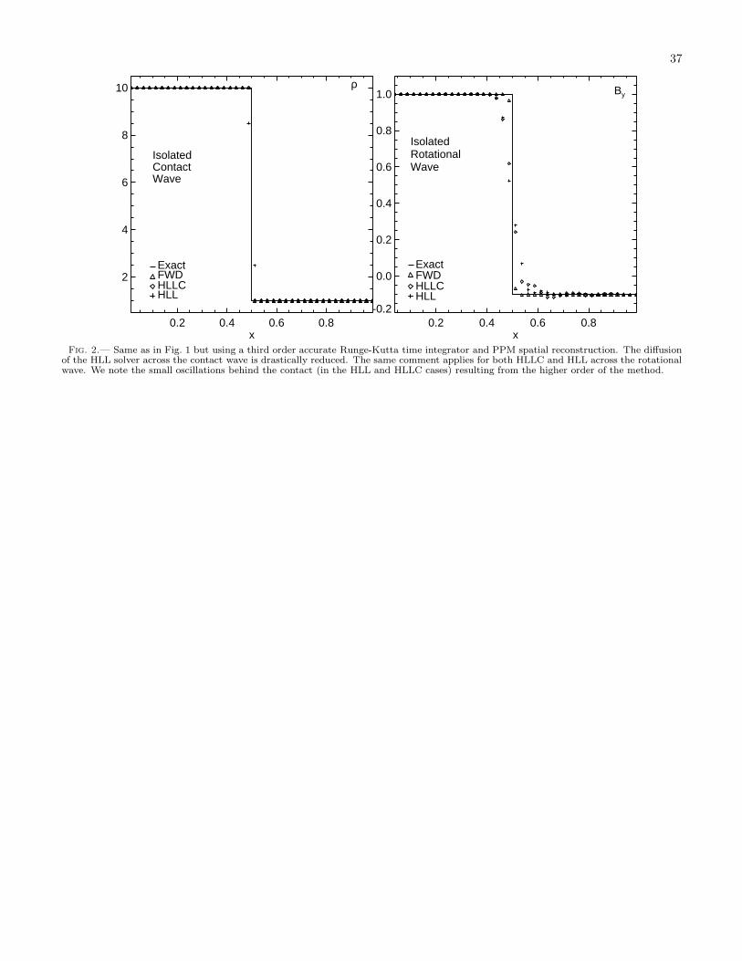
37

0.2 0.4 0.6 0.8x

-0.2

0.0

0.2

0.4

0.6

0.8

1.0 By

IsolatedRotationalWave

HLLHLLCFWDExact

0.2 0.4 0.6 0.8x

2

4

6

8

10 ρ

IsolatedContactWave

HLLHLLCFWDExact

Fig. 2.— Same as in Fig. 1 but using a third order accurate Runge-Kutta time integrator and PPM spatial reconstruction. The diffusionof the HLL solver across the contact wave is drastically reduced. The same comment applies for both HLLC and HLL across the rotationalwave. We note the small oscillations behind the contact (in the HLL and HLLC cases) resulting from the higher order of the method.

38

0.2 0.4 0.6 0.8x

0.2

0.4

0.6

0.8

1.0 ρ

HLL

HLLC

FWD

Exact0.2 0.4 0.6 0.8x

0.2

0.4

0.6

0.8

1.0 Pg

0.2 0.4 0.6 0.8x

0.8

1.0

1.2

1.4

1.6 P

0.2 0.4 0.6 0.8x

0.0

0.1

0.2

0.3

0.4Vx

0.2 0.4 0.6 0.8x

-0.6

-0.4

-0.2

0.0Vy

0.2 0.4 0.6 0.8x

-1.0

-0.5

0.0

0.5

1.0 By

Fig. 3.— Relativistic Brio-Wu shock tube test at t = 0.4. Computations are carried on 400 zones using the FWD (dashed-dotted line),HLLC (dashed line), HLL (dotted-crossed line) and exact (solid line) Riemann solver, respectively. The top panel shows, from left toright, the rest-mass density, gas pressure, total pressure. In the bottom panel the x and y components of velocity and the y componentof magnetic field are shown. The compound wave in the numerical solution between the fast left-propagating rarefaction and the contactdiscontinuity (at x ≈ 0.51 in the plots) is not captured in the analytical solution provided by Giacomazzo & Rezzolla (2006) that avoidsthis kind of solution by construction.

39

0.50 0.55 0.60 0.65 0.70x

0.2

0.4

0.6

0.8

ρ

HLL

HLLC

FWD

Exact

0.50 0.55 0.60 0.65 0.70x

0.0

0.1

0.2

0.3

Vx

0.50 0.55 0.60 0.65 0.70x

-0.6

-0.4

-0.2

0.0Vy

Fig. 4.— Zoom of the central region of Fig.3, focusing on the compound wave (at x ≃ 0.51), the contact discontinuity (at x ≃ 0.60) andthe right-going slow shock (at x ≃ 0.65). From left to right, we show the rest-mass density and the two components of velocity.

40

100 1000

1

10Shock Tube 1

εL1(ρ) x 102

HLLHLLCFWD

100 1000

1

10

Shock Tube 2εL1(By) x 102

100 10001/∆x

10

100

Shock Tube 3

εL1(By) x 102

100 10001/∆x

0.1

1.0

Shock Tube 4εL1(ρ) x 102

Fig. 5.— L-1 norm errors (in 102) for the four shock tube problems of Table 1 as function of the grid resolution ∆x = 1/Nx. The differentcombinations of lines and symbols refer to FWD (solid, diamonds), HLLC (dashed, crosses) and HLL (dotted, plus signs).

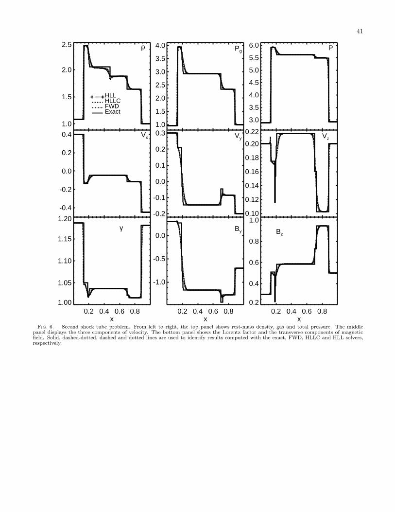
41

0.2 0.4 0.6 0.8x

1.0

1.5

2.0

2.5 ρ

HLLHLLCFWDExact

0.2 0.4 0.6 0.8x

1.0

1.5

2.0

2.5

3.0

3.5

4.0 Pg

0.2 0.4 0.6 0.8x

3.0

3.5

4.0

4.5

5.0

5.5

6.0 P

0.2 0.4 0.6 0.8x

-0.4

-0.2

0.0

0.2

0.4 Vx

0.2 0.4 0.6 0.8x

-0.2

-0.1

0.0

0.1

0.2

0.3 Vy

0.2 0.4 0.6 0.8x

0.10

0.12

0.14

0.16

0.18

0.20

0.22Vz

0.2 0.4 0.6 0.8x

1.00

1.05

1.10

1.15

1.20γ

0.2 0.4 0.6 0.8x

-1.0

-0.5

0.0By

0.2 0.4 0.6 0.8x

0.2

0.4

0.6

0.8

1.0

Bz

Fig. 6.— Second shock tube problem. From left to right, the top panel shows rest-mass density, gas and total pressure. The middlepanel displays the three components of velocity. The bottom panel shows the Lorentz factor and the transverse components of magneticfield. Solid, dashed-dotted, dashed and dotted lines are used to identify results computed with the exact, FWD, HLLC and HLL solvers,respectively.

42

0.42 0.44 0.46 0.48 0.50x

1.85

1.90

1.95

2.00

2.05 ρ

HLLHLLCFWDExact

0.68 0.70 0.72 0.74 0.76x

0.10

0.12

0.14

0.16

0.18

0.20

0.22Vz

0.68 0.70 0.72 0.74 0.76x

-1.40

-1.35

-1.30

-1.25

-1.20By

Fig. 7.— Left panel: closer look of the rest-mass density of Fig. 6 around the contact wave. Middle and right panels: enlargements ofthe z component of velocity and y component of magnetic field around the right-going slow shock and Alfven discontinuity, respectively.

43

0.2 0.4 0.6 0.8x0

10

20

30

40

50

60 ρ

0.2 0.4 0.6 0.8x0

200

400

600

800

1000

1200 Pg

0.2 0.4 0.6 0.8x0

200

400

600

800

1000

1200 P

0.2 0.4 0.6 0.8x

-1.0

-0.5

0.0

0.5

1.0 Vx

HLLHLLCFWDExact

0.2 0.4 0.6 0.8x

-0.30

-0.25

-0.20

-0.15

-0.10

-0.05

-0.00

0.05Vy

0.2 0.4 0.6 0.8x

-10

0

10

By

Fig. 8.— Results of the shock tube 3 (Table 1) using different solvers. From top to bottom, left to right, the panels show rest-massdensity, gas pressure, total pressure, x and y components of velocity and y component of magnetic field. The exact solution of this Riemannproblem is plotted with a solid line. Dash-dotted, dashed and dotted lines refer to the results obtained with FWD, HLLC and HLL solvers,respectively.

0.40 0.45 0.50 0.55 0.60x

40

45

50

55

60ρ

HLLHLLCFWDExact

0.40 0.45 0.50 0.55 0.60x

-0.30

-0.25

-0.20

-0.15

-0.10

-0.05

-0.00

0.05Vy

0.40 0.45 0.50 0.55 0.60x

-10

0

10

By

Fig. 9.— Closer view of the central region of Fig.8. Type lines have the same meaning as in Fig.7. The rest-mass density is representedin the left panel, where the wall heating pathology is notorious. Central and right panels show the profiles transverse components of thevelocity and of the magnetic field, respectively.

44

0.2 0.4 0.6 0.8x0.9

1.0

1.1

1.2

ρ

0.2 0.4 0.6 0.8x

4.5

5.0

5.5

6.0

6.5

7.0

7.5 Pg

0.2 0.4 0.6 0.8x20

21

22

23

24P

0.2 0.4 0.6 0.8x

0.00

0.02

0.04

0.06Vx

HLL

HLLC

FWD

Exact0.2 0.4 0.6 0.8x

0.0

0.1

0.2

0.3 Vy

0.2 0.4 0.6 0.8x

0.0

0.1

0.2

0.3

0.4 Vz

0.2 0.4 0.6 0.8x

1.00

1.05

1.10

1.15

1.20γ

0.2 0.4 0.6 0.8x

5.0

5.2

5.4

5.6

5.8

6.0By

0.2 0.4 0.6 0.8x

0.8

1.0

1.2

1.4

1.6

1.8

2.0Bz

Fig. 10.— Same as Fig. 6, but for the general Alfven test (Table 1).

45

0.40 0.45 0.50 0.55 0.60x

0.9

1.0

1.1

1.2

ρ

0.40 0.45 0.50 0.55 0.60x

0.0

0.1

0.2

0.3

Vy

HLLHLLCFWDExact

0.40 0.45 0.50 0.55 0.60x

5.1

5.2

5.3

5.4

5.5

5.6

5.7By

Fig. 11.— Enlargement of the central region of Fig.10 where the profiles of the rest-mass density (left), vy (middle) and By are displayed.The contact wave at x ≃ 0.52 separating the two slow shocks is better captured by the FWD solver. Both HLLC and FWD solversundershoot the true solution to the right of the contact wave. The Alfven modes at x ≈ 0.44 and x ≈ 0.58 are not fully smeared at thisresolution using the FWD solver, although they are obviously unresolved using 800 uniform numerical zones.

HLLC FWD

W

W

W

W

Fig. 12.— Ultrarelativistic shell at t = 3.5 (simulation units, which correspond to 1.1× 106 s) run with 32000 numerical zones (Table 1).The left and right panels show the results using HLLC and FWD solvers, respectively. Different line styles are used to display a numberof physical variables.

46

b c

e f

a

d

Fig. 13.— The rest-mass density distribution of the two-dimensional cylindrical explosion problem at t = 4.0. The upper (bottom) panelshave been run with a grid of 800× 800 (400× 400) numerical zones, a CFL number 0.4 (0.6), PPM spatial reconstruction and a third-orderaccurate Runge-Kutta integration scheme. Left, middle and right panels show the results obtained using FWD, HLLC and HLL solvers,respectively.

b c

e f

a

d

Fig. 14.— The rest-mass density distribution of the two-dimensional rotor problem at t = 4.0. The upper (bottom) panels have been runwith a resolution of 10242 (1282). Left, middle and right panels show the results obtained using FWD, HLLC and HLL solvers, respectively.

47

Fig. 15.— Characteristic wavespeeds. Ideal gas with γ = 4/3. Dashed lines correpond to fast magnetosonic waves, continuous lines toAlfven wavespeeds, and dash-dotted lines to slow magnetosonic waves. Top-left panel: Fluid at rest with ρ = 1.0, ε = 1.0, Bx = 5.0,By = 0.0, Bz = 0.0. Top-right panel: Fluid at rest with ρ = 1.0, ε = 50.0, Bx = 5.0, By = 0.0, Bz = 0.0. Bottom-left panel: Fluid atrest with ρ = 1.0, ε = 37.864, Bx = 5.0, By = 0.0, Bz = 0.0. In these three panels, the curve associated to the entropy wave degeneratesin a point located at the origin, and Type I degeneracy is along y axis, whereas the three subcases of Type II degeneracy are along thex axis. Bottom-right panel: Fluid state as in the top-right panel but moving along the x-axis at a speed vx = 0.9. Entropic wavespeedcorresponds to dash-triple-dotted line. Type I and II degeneracies are again along y and x axis, respectively.

48

Fig. 16.— Characteristic wavespeeds. Ideal gas with γ = 4/3, ρ = 1.0, ε = 1.0, vx = 0.0, vy = −0.50, vz = 0.0, Bx = 5.0, By = 0.0,Bz = 0.0. Line types as in Fig. 15. Left panel: xy-plane. Type I degeneracy is along y axis. Type II degeneracy is along the directionspointed by the arrows. Right panel: xz-plane. Type I degeneracy is along z axis. There is no Type II degeneracy on this plane.

Fig. 17.— Characteristic wavespeeds. Ideal gas with γ = 4/3, ρ = 1.0, ε = 1.0, vx = 0.634, vy = 0.634, vz = 0.0, Bx = 5.0, By = 0.0,Bz = 0.0. Line types as in Fig. 15. Left panel: xy-plane. Type I degeneracy is along y axis. Type II degeneracy is along the directionspointed by the arrows. Right panel: xz-plane. Type I degeneracy is along z axis. There is no Type II degeneracy on this plane.

49

TABLE 1Initial conditions for the test problems of Sect. 8.1

Test State ρ pg vx vy vz Bx By Bz Time Zones

Contact WaveL 10 1 0 0.7 0.2 5 1 0.5

1 40R 1 1 0 0.7 0.2 5 1 0.5

Rotational WaveL 1 1 0.4 −0.3 0.5 2.4 1 −1.6

1 40R 1 1 0.377347 −0.482389 0.424190 2.4 −0.1 −2.178213

Shock Tube 1L 1 1 0 0 0 0.5 1 0

0.4 400R 0.125 0.1 0 0 0 0.5 −1 0

Shock Tube 2L 1.08 0.95 0.4 0.3 0.2 2 0.3 0.3

0.55 800R 1 1 −0.45 −0.2 0.2 2 −0.7 0.5

Shock Tube 3L 1 0.1 0.999 0 0 10 7 7

0.4 400R 1 0.1 −0.999 0 0 10 −7 −7

Shock Tube 4L 1 5 0 0.3 0.4 1 6 2

0.5 800R 0.9 5.3 0 0 0 1 5 2

UR shellL 10−3 10−5 0 0 0 0 0 0

3.5 32000M 1 2.5 × 10−3 0.997775 0 0 0 4.60706 0R 3.297 × 10−4 8.2424 × 10−7 0.997775 0 0 0 0 0

Note. — The last two columns give, respectively, the time at which the solution is shown in the figures and the number of numericalzones used in the computation. The last test is set up in spherical coordinates, and the vector components (x, y, z) correspond to thespherical ones (r, φ, θ)

50

TABLE 2CPU times for the two-dimensional

rotor problem.

Resolution tHLLC/tHLL tFWD/tHLL

1282 1.75 2.532562 1.45 2.845122 1.08 1.5010242 1.13 1.93

Note. — Execution times for test casesrun with the HLLC and FWD solvers arenormalized to those corresponding to theHLL solver. In all cases the third-orderscheme with a Courant number 0.3 has beenused