The Geometry of Wulff Crystal Shapes and Its Relations with Riemann Problems
Upload
independentCategory
view
0download
0
arX
iv:1
107.
6036
v2 [
mat
h.SP
] 6
Nov
201
1
THE HESSENBERG MATRIX AND THE RIEMANN MAPPINGFUNCTION
C. ESCRIBANO, A. GIRALDO, M. A. SASTRE, AND E. TORRANO
Abstract. We consider a Jordan arc Γ in the complex plane C and a regularmeasure µ whose support is Γ. We denote by D the upper Hessenberg matrixof the multiplication by z operator with respect to the orthonormal polynomialbasis associated with µ. We show in this work that, if the Hessenberg matrix D
is uniformly asymptotically Toeplitz, then the symbol of the limit operator is therestriction to the unit circle of the Riemann mapping function φ(z) which mapsconformally the exterior of the unit disk onto the exterior of the support of themeasure µ.
We use this result to show how to approximate the Riemann mapping functionfor the support of µ from the entries of the Hessenberg matrix D.
1. Introduction
In this paper, we consider regular measures µ defined on subsets of the complexplane that are Jordan arcs, or finite union of Jordan arcs such that its complementis simply connected, and we show how the entries of the Hessenberg matrix D asso-ciated with µ determines the Riemann mapping function that takes the complementof the closed unit disk D to the complement of the support of µ.
The Riemann mapping theorem says, in its most common statement (see, forexample, [1]), that given a simply connected domain Ω ( C and given z0 ∈ Ω, thereis a unique analytic map φ : Ω −→ D (D the open unit disk), normalized by theconditions φ(z0) = 0 and φ′(z0) > 0, such that φ defines a one-to-one mapping of Ωonto D. However, we will use an equivalent formulation for domains containing ∞which can be found, for example, in [28, 22, 18]. In this case, the Riemann mappingtheorem states that, for every Γ ⊂ C compact that is not a point, such that C∞ \Γis simply connected, there is a unique conformal mapping φ : C∞ \ D → C∞ \Γsuch that φ(∞) = ∞ and φ′(∞) > 0, where φ′(∞) = cap(Γ), the capacity of Γ.Moreover, if Γ is a simple Jordan curve, φ(z) is continuous in the unit circle T.
There exists a well-known link between the Riemann mapping function and theGreen function, which has been described in the literature on potential theory (see,for example, [11]). If we denote by Φ(z) the inverse of φ(z) as defined in the previousparagraph, then the Green function for a compact set K with cap(K) > 0, gK(z,∞),can be obtained from the Riemann conformal mapping Φ(z) which takes C∞ \Pc(K)onto the exterior of D, where Pc(K) is the polynomial convex hull of K. Moreover,
if Φ(z) =
∞∑
k=−1
c−kz−k, c1 > 0, in a neighborhood of ∞, then
gK(z,∞) =
log |Φ(z)| if z ∈ C∞ \Pc(K)0 otherwise.
1

2 C. ESCRIBANO, A. GIRALDO, M. A. SASTRE, AND E. TORRANO
In particular, c1 =1
cap(K).
An infinite matrix T = (ai,j)∞i,j=1 is a Toeplitz matrix if each descending diagonal
from left to right is constant, i.e, there exists (ai)i∈Z such that
T =
a0 a−1 a−2 . . .a1 a0 a−1 . . .a2 a1 a0 . . .a3 a2 a1 . . ....
......
. . .
.
Given a Toeplitz matrix T , the Laurent series whose coefficients are the entries aidefines a function known as the symbol of T .
J.Barrıa and P.R.Halmos [3] called an operator A on ℓ2 asymptotically Toeplitz ifthe sequence of operators S∗nASn converges strongly to a bounded operator on ℓ2,where S is the forward shift and S∗ its adjoint. Later, A.Feintuch [10] established thedefinitions of weak and uniform operator convergence. Hence there are actually threedifferent kinds of asymptotic toeplitzness. In this work we deal with the uniformone: a bounded operator A on ℓ2 is uniformly asymptotically Toeplitz provided thereis a bounded operator T on ℓ2 such that
limn→∞
‖S∗nASn − T‖ = 0.
By Theorem 2.4 in [10], uniformly asymptotically Toeplitz operators are character-ized as the compact perturbations of Toeplitz operators.
In the real case, the Hessenberg matrix agrees with the tridiagonal Jacobi matrix.Rakhmanov’s theorem [23, 24] states that, if the support of a Borel measure is [−1, 1]with µ′ > 0 almost everywhere in [−1, 1], and
J =
b0 a1 0 . . .a1 b1 a2 . . .0 a2 b2 . . .0 0 a3 . . ....
......
. . .
is the Jacobi matrix associated with µ, then an → 1
2and bn → 0. We observe that
this matrix operator is a compact perturbation of a Toeplitz operator, so that J isuniformly asymptotic Toeplitz.
Note that in this case, the Riemann mapping function for the interval [−1, 1] is
φ(z) =1
2
(z +
1
z
)=
1
2z + 0 +
1
2
1
z
Moreover, under the conditions of Rakhmanov’s theorem, if supp(µ) = [a, b], then
the above limits are an → b− a
4and bn → a+ b
2. In this case, the Riemann mapping
function is
φ(z) =b− a
4z +
a+ b
2+
b− a
4
1
z.
THE HESSENBERG MATRIX AND THE RIEMANN MAPPING FUNCTION 3
Conversely, P.Nevai established in [21] that, if an → a > 0 and bn → b, then thesupport is [−2a + b, b + 2a] ∪ e (where e is at most a denumerable set of isolatedpoints). Moreover, Nevai proved the equivalence between the existence of thoselimits and the ratio asymptotics of orthonormal polynomials.
Generalizations of Rakhmanov’s theorem to orthogonal polynomials, and to or-thogonal matrix polynomials on the unit circle, have been given in [20] and [30].The case of orthogonal polynomials on an arc of circle has been studied in [4].
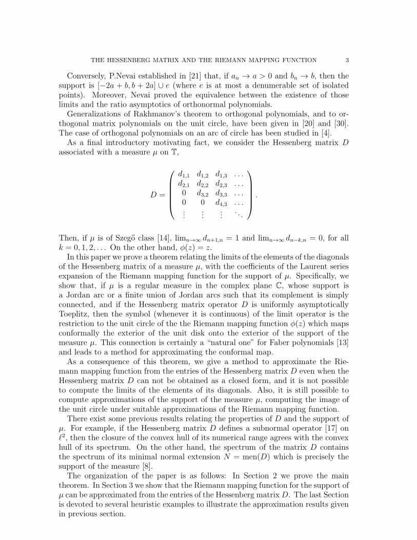
As a final introductory motivating fact, we consider the Hessenberg matrix Dassociated with a measure µ on T,
D =
d1,1 d1,2 d1,3 . . .d2,1 d2,2 d2,3 . . .0 d3,2 d3,3 . . .0 0 d4,3 . . ....
......
. . .
.
Then, if µ is of Szego class [14], limn→∞ dn+1,n = 1 and limn→∞ dn−k,n = 0, for allk = 0, 1, 2, . . . On the other hand, φ(z) = z.
In this paper we prove a theorem relating the limits of the elements of the diagonalsof the Hessenberg matrix of a measure µ, with the coefficients of the Laurent seriesexpansion of the Riemann mapping function for the support of µ. Specifically, weshow that, if µ is a regular measure in the complex plane C, whose support isa Jordan arc or a finite union of Jordan arcs such that its complement is simplyconnected, and if the Hessenberg matrix operator D is uniformly asymptoticallyToeplitz, then the symbol (whenever it is continuous) of the limit operator is therestriction to the unit circle of the the Riemann mapping function φ(z) which mapsconformally the exterior of the unit disk onto the exterior of the support of themeasure µ. This connection is certainly a “natural one” for Faber polynomials [13]and leads to a method for approximating the conformal map.
As a consequence of this theorem, we give a method to approximate the Rie-mann mapping function from the entries of the Hessenberg matrix D even when theHessenberg matrix D can not be obtained as a closed form, and it is not possibleto compute the limits of the elements of its diagonals. Also, it is still possible tocompute approximations of the support of the measure µ, computing the image ofthe unit circle under suitable approximations of the Riemann mapping function.
There exist some previous results relating the properties of D and the support ofµ. For example, if the Hessenberg matrix D defines a subnormal operator [17] onℓ2, then the closure of the convex hull of its numerical range agrees with the convexhull of its spectrum. On the other hand, the spectrum of the matrix D containsthe spectrum of its minimal normal extension N = men(D) which is precisely thesupport of the measure [8].
The organization of the paper is as follows: In Section 2 we prove the maintheorem. In Section 3 we show that the Riemann mapping function for the support ofµ can be approximated from the entries of the Hessenberg matrixD. The last Sectionis devoted to several heuristic examples to illustrate the approximation results givenin previous section.
4 C. ESCRIBANO, A. GIRALDO, M. A. SASTRE, AND E. TORRANO
For general information on the theory of orthogonal polynomials, we recommendthe books [6, 28] by T. S. Chihara and G. Szego, respectively, and the survey [16]by L. Golinskii and V. Totik.
2. The Diagonals Theorem
Let µ be a Borel probability measure in the complex plane, with support supp(µ)containing infinitely many points. Let P be the space of polynomials. The associatedinner product is given by the expression
〈Q(z), R(z)〉µ =
∫
supp(µ)
Q(z)R(z)dµ(z),
forQ,R ∈ P. Then there exists a unique orthonormal polynomials sequence (ONPS)Pn(z)∞n=0 associated to the measure µ [6, 12, 28].
In the space P2(µ), closure of the polynomials space P in L2µ(Ω), we consider the
multiplication by z operator. Let D = (dij)∞i,j=1 be the infinite upper Hessenberg
matrix of this operator in the basis of ONPS Pn(z)∞n=0, hence
(1) zPn(z) =n+1∑
k=0
dk+1,n+1Pk(z), n ≥ 0,
with P0(z) = 1.It is a well-known fact that the monic polynomials are the characteristic polyno-
mials of the finite sections of D.To state our main result, we will require the measure µ to be regular with support
a finite union of Jordan arcs such that its complement is simply connected, and wewill also need to consider an auxiliary Toeplitz matrix. We next recall the definitionsof all these notions.
A Jordan arc in C is any subset of C homeomorphic to the closed interval [0, 1]on the real line.
A measure µ is regular if limn→∞
1n
√γn
= cap(supp(µ)), the capacity of the support
of µ, where the γn are the leading coefficients of the orthonormal polynomials, i.e.,Pn(z) = γnz
n + · · · .We are now in a position to state and prove the main result of the paper.
Theorem 1 (The diagonals theorem). Let D = (dij)∞i,j=1 be the Hessenberg matrix
associated with a measure µ with compact support on the complex plane. Assume
that:
(1) The measure µ is regular with support supp(µ) a Jordan arc or a finite union
of Jordan arcs Γ such that C∞ \Γ is a simply connected set of the Riemann
sphere C∞.
(2) The Hessenberg matrix operator D is uniformly asymptotically Toeplitz and
the corresponding limit matrix T has a continuous symbol.
Then, the symbol of T is the restriction to the unit circle of the the Riemann mapping
function φ : C∞ \D → C∞ \Γ which maps conformally the exterior of the unit disk
onto the exterior of the support of the measure µ.
THE HESSENBERG MATRIX AND THE RIEMANN MAPPING FUNCTION 5
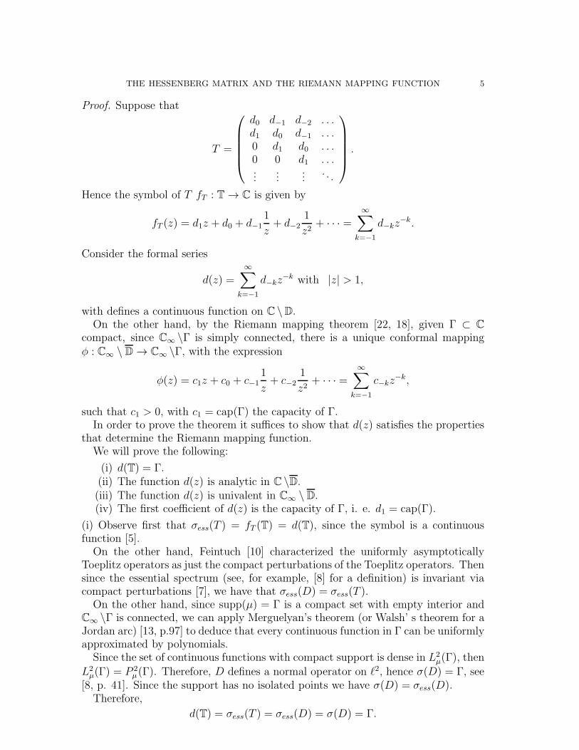
Proof. Suppose that
T =
d0 d−1 d−2 . . .d1 d0 d−1 . . .0 d1 d0 . . .0 0 d1 . . ....
......
. . .
.
Hence the symbol of T fT : T → C is given by
fT (z) = d1z + d0 + d−11
z+ d−2
1
z2+ · · · =
∞∑
k=−1
d−kz−k.
Consider the formal series
d(z) =∞∑
k=−1
d−kz−k with |z| > 1,
with defines a continuous function on C \D.On the other hand, by the Riemann mapping theorem [22, 18], given Γ ⊂ C
compact, since C∞ \Γ is simply connected, there is a unique conformal mappingφ : C∞ \ D → C∞ \Γ, with the expression
φ(z) = c1z + c0 + c−11
z+ c−2
1
z2+ · · · =
∞∑
k=−1
c−kz−k,
such that c1 > 0, with c1 = cap(Γ) the capacity of Γ.In order to prove the theorem it suffices to show that d(z) satisfies the properties
that determine the Riemann mapping function.We will prove the following:
(i) d(T) = Γ.(ii) The function d(z) is analytic in C \D.(iii) The function d(z) is univalent in C∞ \D.(iv) The first coefficient of d(z) is the capacity of Γ, i. e. d1 = cap(Γ).
(i) Observe first that σess(T ) = fT (T) = d(T), since the symbol is a continuousfunction [5].
On the other hand, Feintuch [10] characterized the uniformly asymptoticallyToeplitz operators as just the compact perturbations of the Toeplitz operators. Thensince the essential spectrum (see, for example, [8] for a definition) is invariant viacompact perturbations [7], we have that σess(D) = σess(T ).
On the other hand, since supp(µ) = Γ is a compact set with empty interior andC∞ \Γ is connected, we can apply Merguelyan’s theorem (or Walsh’ s theorem for aJordan arc) [13, p.97] to deduce that every continuous function in Γ can be uniformlyapproximated by polynomials.
Since the set of continuous functions with compact support is dense in L2µ(Γ), then
L2µ(Γ) = P 2
µ(Γ). Therefore, D defines a normal operator on ℓ2, hence σ(D) = Γ, see[8, p. 41]. Since the support has no isolated points we have σ(D) = σess(D).
Therefore,
d(T) = σess(T ) = σess(D) = σ(D) = Γ.
6 C. ESCRIBANO, A. GIRALDO, M. A. SASTRE, AND E. TORRANO
(ii) To show that d(z) = d1z +∞∑
k=0
d−kz−k is analytic in C \D, we have, on the one
hand, that the function given by the first summand d1z is analytic in C. On the
other hand, consider d(z) =
∞∑
k=0
d−kz−k.
If |z| > 1, applying Chauchy-Schwarz inequality we have
∞∑
k=0
∣∣∣∣d−k
zk
∣∣∣∣ ≤
√√√√∞∑
k=0
|d−k|2√√√√
∞∑
k=0
|z|−2k ≤ ||d||2
√1
1− |z|2 < ∞.
Therefore, d(z) is analytic in C \D.(iii) Now, we have that d(z) is analytic in C \D and it is continuous in C \D.Moreover, the set of limit points of d(z) as |z| → 1 agrees with d(T) = Γ whichis bounded, without interior points and does not disconnect C∞. Therefore d(z) isa conformal map in C∞ \D (see [22, Th 1.1]).
(iv) We finally show that d1 = cap(Γ).The elements dn+1,n of the subdiagonal of the matrix D agree with the quotients
γn/γn+1. Since limn→∞
dn+1,n = d1, then
d1 = limn→∞
dn+1,n = limn→∞
γnγn+1
= limn→∞
1n
√γn
.
On the other hand, since µ is regular, then [27]
limn→∞
1n
√γn
= cap(supp(µ)).
Therefore, d1 = cap(supp(µ)) = cap(Γ).
Corollary 1. Let D = (dij)∞i,j=1 be the Hessenberg matrix associated with a measure
µ with compact support on the complex plane. Assume that:
(1) The measure µ is regular with Γ = supp(µ) a Jordan arc or a finite union
of Jordan arcs such that C∞ \Γ is a simply connected set of the Riemann
sphere C∞.
(2) The Hessenberg matrix operator D is uniformly asymptotically Toeplitz and
the corresponding limit matrix T has its rows in ℓ1.
Then, the symbol of T is the restriction to the unit circle of the the Riemann mapping
function φ : C∞ \D → C∞ \Γ which maps conformally the exterior of the unit disk
onto the exterior of the support of the measure µ.
Proof. It is well known that every function∑∞
k=0
∣∣∣∣d−k
zk
∣∣∣∣ with∑∞
k=0 |d−k| ≤ ∞ is
continuous on unit circle |z| = 1.
As an illustration of Theorem 1 we consider the following example.
Example 1 (Arc of circle). We consider Γ an arc of the unit circle T. In thiscase [15] (see also [25, 26]), there exists a regular measure for which the diagonals ofthe Hessenberg matrix stabilize from the second element on. The monic orthogonal

THE HESSENBERG MATRIX AND THE RIEMANN MAPPING FUNCTION 7
polynomials associated to this measure satisfy Ψ0(0) = 1 and Ψn(0) =1
a(a > 1), if
n ≥ 1, and the corresponding Hessenberg matrix is the following unitary matrix D
−1
a−(a2 − 1)1/2
a2−(a2 − 1)2/2
a3−(a2 − 1)3/2
a4−(a2 − 1)4/2
a5· · ·
(a2 − 1)1/2
a− 1
a2−(a2 − 1)1/2
a3−(a2 − 1)2/2
a4−(a2 − 1)3/2
a5· · ·
0(a2 − 1)1/2
a− 1
a2−(a2 − 1)1/2
a3−(a2 − 1)2/2
a4· · ·
0 0(a2 − 1)1/2
a− 1
a2(a2 − 1)1/2
a3· · ·
......
......
.... . .
.
Note that S∗nDSn = T for all n ≥ 1 is a Toeplitz matrix such that the first row is
a geometric series of ratio
√a2 − 1
a< 1 (because a > 1). Hence the rows of T are
in ℓ1.On the other hand,
D − T =
−a− 1
a2−(a2 − 1)1/2(a− 1)
a3−(a2 − 1)(a− 1)
a4. . .
0 0 0 . . .0 0 0 . . ....
......
. . .
,
is compact because it is Hilbert-Schmidt:
√√√√∞∑
i,j=1
|aij|2 =
√√√√∞∑
n=0
((a− 1)(a2 − 1)n/2
a2+n
)2
=a− 1
a< +∞.
Then we have that D = T +K where T is a Toeplitz operator and K is compact,therefore D is asymptotically uniformly Toeplitz [10] and the hypothesis of Theorem1 are satisfied. Then, the expression of the Riemann mapping function as a Laurentseries is
φ(z) =z(a−
√a2 − 1 z
)√a2 − 1− az
=
√a2 − 1
az −
∞∑
n=0
(a2 − 1)n
2
an+2z−n.

8 C. ESCRIBANO, A. GIRALDO, M. A. SASTRE, AND E. TORRANO
Figure 1. The Riemann mapping function for the arc for a = 2
3. Approximation of the Riemann mapping function
When the Hessenberg matrix D can not obtained as a closed form and it is notpossible to compute the limits of the elements of its diagonals, we may ask if it isstill possible to compute approximations of the Riemann mapping function.
Specifically, under the hypothesis of theorem 1, since the coefficients of the Rie-mann mapping function are the limits of the elements in each of the diagonals ofthe Hessenberg matrix, we may ask if the functions
hn(z) = dn+1,nz + dn,n +dn−1,n
z+
dn−2,n
z2+ . . .+
d1,nzn−1
,
defined from the n-th column cn of the Hessenberg matrix, are suitable approxima-tions of the Riemann mapping function φ(z).
We show in this section that this is indeed the case.In what follows we will denote by Θn the norm in ℓ2 the of n-th column of the
matrix D − T as a vector of ℓ2, i.e.,
Θn =
√√√√n−1∑
k=−1
|d−k − dn−k,n|2.
Lemma 1. Suppose that D is an asymptotically uniformly Toeplitz operator on ℓ2.Then
limn→∞
Θn = 0.
Proof. Note that D−T is a compact operator [10]. Since en is a sequence weaklyconvergent to 0, then (D − T )en−1 converges strongly to 0.
Therefore, Θn = ‖(D − T )en−1‖2 → 0.
Theorem 2. Under the hypothesis of Theorem 1, the sequence of functions
hn(z) = dn+1,nz + dn,n +dn−1,n
z+
dn−2,n
z2+ . . .+
d1,nzn−1
converges uniformly to the Riemann mapping function φ(z) on any compact set
K ⊂ C \D.

THE HESSENBERG MATRIX AND THE RIEMANN MAPPING FUNCTION 9
Proof. Consider a compact subset K ⊂ C \D and consider ε > 0. Since K iscompact, there exist r, R ∈ R such that 1 < r ≤ |z| ≤ R for every z ∈ K.
For every z ∈ K, we have
|hn(z)− φ(z)| =
=
∣∣∣∣(d1 − dn+1,n)z + (d0 − dn,n) +d−1 − dn−1,n
z+ · · ·
· · ·+ d1−n − d1,nzn−1
+
∞∑
k=n
d−k1
z−k
∣∣∣∣∣
≤n−1∑
k=−1
∣∣∣∣d−k − dn−k,n
zk
∣∣∣∣+∞∑
k=n
∣∣∣∣d−k
zk
∣∣∣∣ .(2)
Applying Cauchy-Schwarz inequality to the second summand of inequality 2, wehave
∞∑
k=n
∣∣∣∣d−k
zk
∣∣∣∣ ≤
√√√√∞∑
k=n
|d−k|2√√√√
∞∑
k=n
|z|−2k ≤√
1
r2 − 1
√√√√∞∑
k=n
|d−k|2.
The last factor is the tail of a vector in ℓ2. Therefore, given ε > 0, there exists
N0 ∈ N such that, for every n < N0,√∑∞
k=n |d−k|2 <√r2 − 1
ε
2.
In a similar way, for the first summand of inequality (2), we have
n−1∑
k=−1
∣∣∣∣d−k − dn−k,n
zk
∣∣∣∣ ≤
√√√√n−1∑
k=−1
|d−k − dn−k,n|2√√√√
n−1∑
k=−1
|z|−2k = Θn
√√√√n−1∑
k=−1
|z|−2k.
Then, for every z ∈ K,
n−1∑
k=−1
|z|−2k ≤ R2 +
∞∑
k=0
r−2k = R2 +1
r2 − 1= C.
Since Θn converges to zero, there exists N1 ∈ N such that, for every n > N1,
Θn <ε
2√C.
Taking N = maxN0, N1 we have that
|hn(z)− φ(z)| < ǫ
for every z ∈ K, for every n > N .
Remark 1. Under the hypothesis of Theorem 1 we consider the sequence cn∞n=1 ofcolumn vectors of the matrix D−T . Since every cn has at most n non null elements,we can calculate its norm in ℓ1 and in ℓ2. We denote these norms by θn and Θn:
θn = ‖cn‖1 =n∑
k=−1
|dn−k,n − d−k|,
Θn = ‖cn‖2 =
√√√√n∑
k=−1
|dn−k,n − d−k|2.
10 C. ESCRIBANO, A. GIRALDO, M. A. SASTRE, AND E. TORRANO
Theorem 2 assures the uniform convergence of hn(z) to the Riemann mappingfunction φ(z) on any compact set K ⊂ C \D.
Now we analyse this convergence when z = reiθ for r ≥ 1.
i) For r > 1, applying Cauchy-Schwarz inequality we have
|hn(reiθ)− φ(reiθ)| ≤
n−1∑
k=−1
∣∣∣∣d−k − dn−k,n
zk
∣∣∣∣ +∞∑
k=n
∣∣∣∣d−k
zk
∣∣∣∣
≤ Θn
√r2 +
1
r2 − 1+ ||φ||2
r√r2 − 1
1
rn.
Therefore, on each circle of radius r, the order of convergence of hn to φwill be at least that of Θn to zero because the other summand is of the orderof 1
rn, r > 1.
ii) For r = 1, we need some additional hypothesis. Under the hypothesis ofCorollary 1, the coefficients of φ are in ℓ1. Now we have
|hn(eiθ)− φ(eiθ)| ≤
n−1∑
k=−1
|d−k − dn−k,n|+∞∑
k=n
|d−k| ≤ θn +
∞∑
k=n
|d−k|
The last summand is the tail of a vector in ℓ1 which goes to zero. Then,the convergence θn −→ 0 assures the convergence of hn −→ φ on the unitcircle.
Theorem 3. Under the hypothesis of Theorem 1, for every ε > 0 there is a δ > 0such that for every r ∈ (1, δ + 1) there is a natural number N , such that for all
n ≥ N we have
|hn(reiθ)− φ(eiθ)| ≤ ε,
for every θ ∈ [0, 2π].
Proof. Consider ε > 0. Consider the compact set K = z : 1 ≤ |z| ≤ 2. Since thefunction φ(z) is uniformly continuous in K, there exists δ > 0, such that for everyr ∈ [1, 1 + δ), we have
|φ(reiθ)− φ(eiθ)| < ε
2,
for every θ ∈ [0, 2π].We consider now, for every r ∈ (1, 1+ δ), the compact set Kr = z ∈ C : |z| = r.
By the uniform convergence of hn on compact sets of C \D, established in Proposition1, there exists n ∈ N such that, for every n ≥ N , we have
|hn(reiθ)− φ(reiθ)| < ε
2
for all θ ∈ [0, 2π]. Then,
|hn(reiθ)− φ(eiθ)| ≤ |hn(re
iθ)− φ(reiθ)|+ |φ(reiθ)− φ(eiθ)| ≤ ε
for every θ ∈ [0, 2π]
We will use this result, in the last section, to approximate the support of themeasure by equipotential curves of the function hn(re
iθ), for suitable n and r.
THE HESSENBERG MATRIX AND THE RIEMANN MAPPING FUNCTION 11
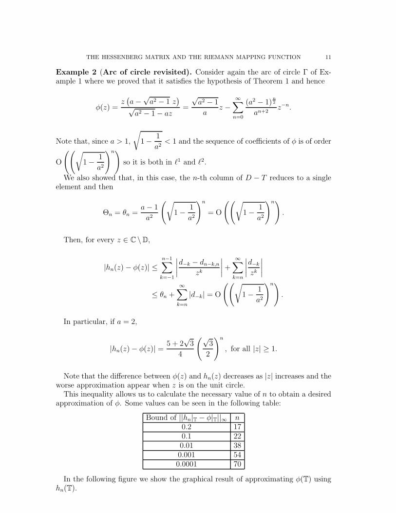
Example 2 (Arc of circle revisited). Consider again the arc of circle Γ of Ex-ample 1 where we proved that it satisfies the hypothesis of Theorem 1 and hence
φ(z) =z(a−
√a2 − 1 z
)√a2 − 1− az
=
√a2 − 1
az −
∞∑
n=0
(a2 − 1)n
2
an+2z−n.
Note that, since a > 1,
√1− 1
a2< 1 and the sequence of coefficients of φ is of order
O
((√1− 1
a2
)n)so it is both in ℓ1 and ℓ2.
We also showed that, in this case, the n-th column of D − T reduces to a singleelement and then
Θn = θn =a− 1
a2
(√1− 1
a2
)n
= O
((√1− 1
a2
)n).
Then, for every z ∈ C \D,
|hn(z)− φ(z)| ≤n−1∑
k=−1
∣∣∣∣d−k − dn−k,n
zk
∣∣∣∣+∞∑
k=n
∣∣∣∣d−k
zk
∣∣∣∣
≤ θn +
∞∑
k=n
|d−k| = O
((√1− 1
a2
)n).
In particular, if a = 2,
|hn(z)− φ(z)| = 5 + 2√3
4
(√3
2
)n
, for all |z| ≥ 1.
Note that the difference between φ(z) and hn(z) decreases as |z| increases and theworse approximation appear when z is on the unit circle.
This inequality allows us to calculate the necessary value of n to obtain a desiredapproximation of φ. Some values can be seen in the following table:
Bound of ||hn|T − φ|T||∞ n0.2 170.1 220.01 380.001 540.0001 70
In the following figure we show the graphical result of approximating φ(T) usinghn(T).
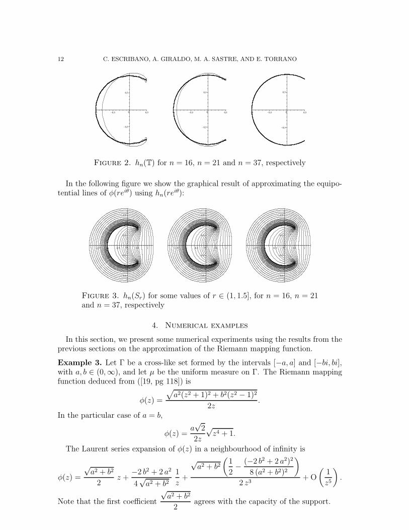
12 C. ESCRIBANO, A. GIRALDO, M. A. SASTRE, AND E. TORRANO
Figure 2. hn(T) for n = 16, n = 21 and n = 37, respectively
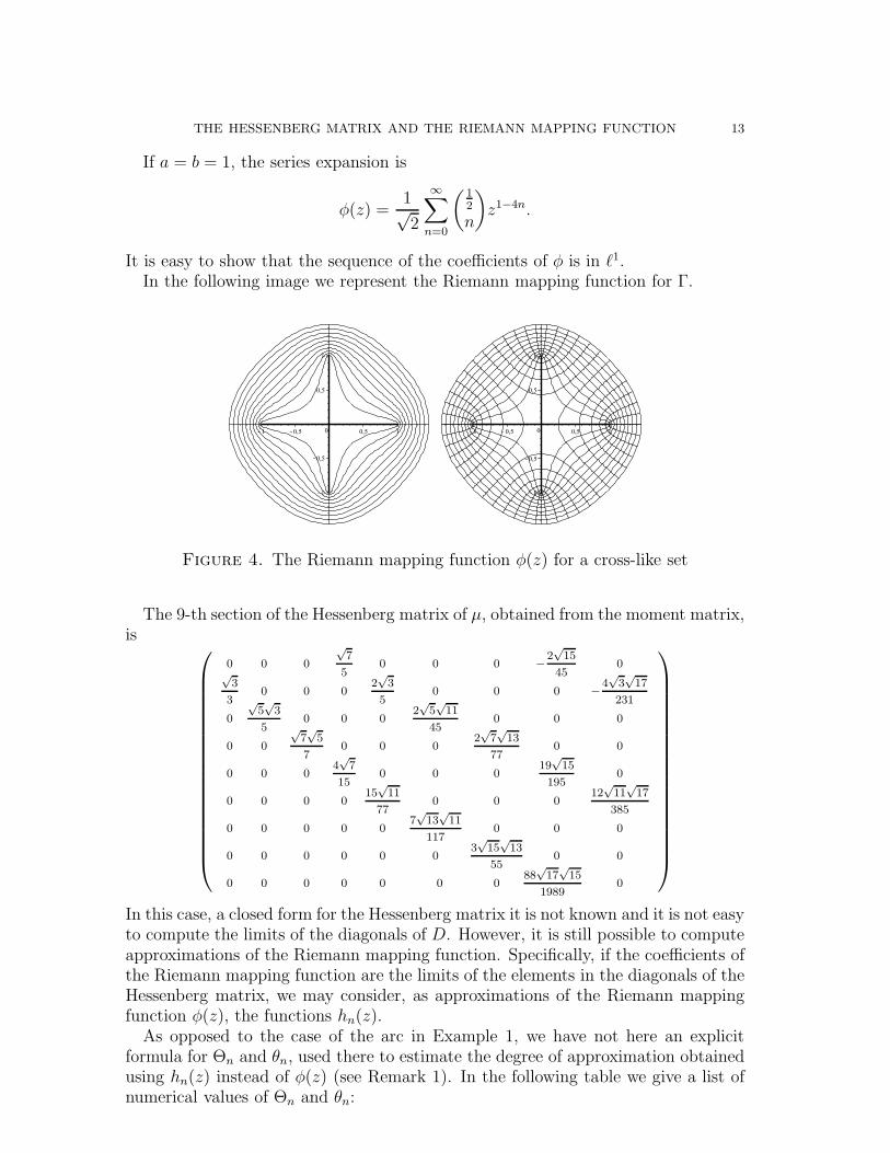
In the following figure we show the graphical result of approximating the equipo-tential lines of φ(reiθ) using hn(re
iθ):
Figure 3. hn(Sr) for some values of r ∈ (1, 1.5], for n = 16, n = 21and n = 37, respectively
4. Numerical examples
In this section, we present some numerical experiments using the results from theprevious sections on the approximation of the Riemann mapping function.
Example 3. Let Γ be a cross-like set formed by the intervals [−a, a] and [−bi, bi],with a, b ∈ (0,∞), and let µ be the uniform measure on Γ. The Riemann mappingfunction deduced from ([19, pg 118]) is
φ(z) =
√a2(z2 + 1)2 + b2(z2 − 1)2
2z.
In the particular case of a = b,
φ(z) =a√2
2z
√z4 + 1.
The Laurent series expansion of φ(z) in a neighbourhood of infinity is
φ(z) =
√a2 + b2
2z +
−2 b2 + 2 a2
4√a2 + b2
1
z+
√a2 + b2
(1
2− (−2 b2 + 2 a2)2
8 (a2 + b2)2
)
2 z3+O
(1
z5
).
Note that the first coefficient
√a2 + b2
2agrees with the capacity of the support.
THE HESSENBERG MATRIX AND THE RIEMANN MAPPING FUNCTION 13
If a = b = 1, the series expansion is
φ(z) =1√2
∞∑
n=0
(12
n
)z1−4n.
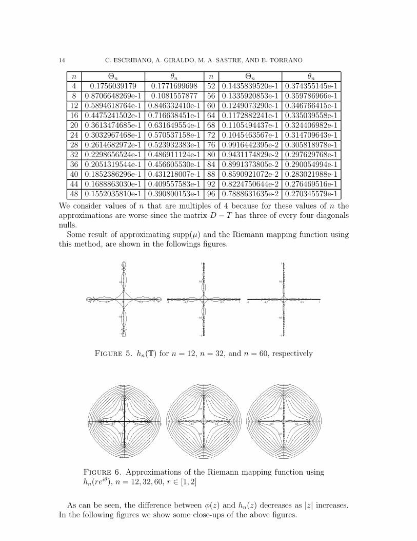
It is easy to show that the sequence of the coefficients of φ is in ℓ1.In the following image we represent the Riemann mapping function for Γ.
Figure 4. The Riemann mapping function φ(z) for a cross-like set
The 9-th section of the Hessenberg matrix of µ, obtained from the moment matrix,is
0 0 0
√7
50 0 0 −
2√15
450
√3
30 0 0
2√3
50 0 0 −
4√3√17
231
0
√5√3
50 0 0
2√5√11
450 0 0
0 0
√7√5
70 0 0
2√7√13
770 0
0 0 04√7
150 0 0
19√15
1950
0 0 0 015
√11
770 0 0
12√11
√17
385
0 0 0 0 07√13
√11
1170 0 0
0 0 0 0 0 03√15
√13
550 0
0 0 0 0 0 0 088
√17
√15
19890
In this case, a closed form for the Hessenberg matrix it is not known and it is not easyto compute the limits of the diagonals of D. However, it is still possible to computeapproximations of the Riemann mapping function. Specifically, if the coefficients ofthe Riemann mapping function are the limits of the elements in the diagonals of theHessenberg matrix, we may consider, as approximations of the Riemann mappingfunction φ(z), the functions hn(z).
As opposed to the case of the arc in Example 1, we have not here an explicitformula for Θn and θn, used there to estimate the degree of approximation obtainedusing hn(z) instead of φ(z) (see Remark 1). In the following table we give a list ofnumerical values of Θn and θn:
14 C. ESCRIBANO, A. GIRALDO, M. A. SASTRE, AND E. TORRANO
n Θn θn n Θn θn4 0.1756039179 0.1771699698 52 0.1435839520e-1 0.374355145e-18 0.8706648269e-1 0.1081557877 56 0.1335920853e-1 0.359786966e-112 0.5894618764e-1 0.846332410e-1 60 0.1249073290e-1 0.346766415e-116 0.4475241502e-1 0.716638451e-1 64 0.1172882241e-1 0.335039558e-120 0.3613474685e-1 0.631649554e-1 68 0.1105494437e-1 0.324406982e-124 0.3032967468e-1 0.570537158e-1 72 0.1045463567e-1 0.314709643e-128 0.2614682972e-1 0.523932383e-1 76 0.9916442395e-2 0.305818978e-132 0.2298656524e-1 0.486911124e-1 80 0.9431174829e-2 0.297629768e-136 0.2051319544e-1 0.456605530e-1 84 0.8991373805e-2 0.290054994e-140 0.1852386296e-1 0.431218007e-1 88 0.8590921072e-2 0.283021988e-144 0.1688863030e-1 0.409557583e-1 92 0.8224750644e-2 0.276469516e-148 0.1552035810e-1 0.390800153e-1 96 0.7888631635e-2 0.270345579e-1
We consider values of n that are multiples of 4 because for these values of n theapproximations are worse since the matrix D − T has three of every four diagonalsnulls.
Some result of approximating supp(µ) and the Riemann mapping function usingthis method, are shown in the followings figures.
Figure 5. hn(T) for n = 12, n = 32, and n = 60, respectively
Figure 6. Approximations of the Riemann mapping function usinghn(re
iθ), n = 12, 32, 60, r ∈ [1, 2]
As can be seen, the difference between φ(z) and hn(z) decreases as |z| increases.In the following figures we show some close-ups of the above figures.

THE HESSENBERG MATRIX AND THE RIEMANN MAPPING FUNCTION 15
Figure 7. Approximations of the Riemann mapping function usinghn(re
iθ), n = 12, 32, 60, r ∈ [1, 1.1]
Example 4. In the following example we take Γ as the half part of a drop-like setof parametric equation
z(t) =(eit)2
1 + 2eit, t ∈ [0, π],
and µ the uniform measure on Γ.Although in this case we do not know if the matrix D − T defines a compact
operator, the following figures seem to indicate that the convergence of hn(T) is veryfast to Γ. In the following figure we show several approximations of the support ofµ using this method.
Figure 8. hn(T) for n = 5, n = 8 and n = 11, respectively
Example 5. For the last example we take Γ as the spiral with parametric equation
z(t) = teit
6, t ∈ [0, 2π]
and we consider µ the uniform measure on Γ.Although in this case we do not know if the matrix D − T defines a compact
operator, the following figures seem to indicate that the convergence of hn(T) toΓ is worse than in the previous example. In the following figure we show severalapproximations of the support of µ using this method.

16 C. ESCRIBANO, A. GIRALDO, M. A. SASTRE, AND E. TORRANO
Figure 9. hn(T) for n = 7 and n = 11, respectively
Acknowledgements
The authors have been supported by Comunidad Autonoma de Madrid and Uni-versidad Politecnica de Madrid (UPM-CAM Q061010133).
References
[1] L. Ahlfors, Complex analysis, McGraw-Hill, 1979.[2] N. I. Akhiezer and I. M. Glazman, Theory of linear operators in Hilbert space, Vol.I and II,
Pitman, London, 1981.[3] J. Barrıa and P. R. Halmos, Asymptotic Toeplitz operators, Trans. Amer. Math. Soc., 92
(1982) 621-630.[4] M. Bello and G. Lopez, Ratio and relative asymptotics of polynomials orthogonal on an arc of
the unit circle, J. Approx. Theory, 92 (1998) 216-244.[5] A. Bottcher and S. M. Grudsky, Spectral properties of banded Toeplitz matrices, SIAM,
Philadelphia, 2005.[6] T. S. Chihara, An introduction to orthogonal polynomials, Gordon and Breach, New York,
1978.[7] J. B. Conway, A course in functional analysis, Graduate Texts in Mathematics, Springer-
Verlag, New York, 1985.[8] J. B. Conway, The theory of subnormal operators, Mathematical Surveys and Monographs,
vol. 36, AMS, Providence, Rhode Island, 1985.[9] P. L. Duren, Theory of Hp spaces, Dover, New York, 1970.
[10] A. Feintuch, On asymptotic Toeplitz and Hankel operators, Operator Theory, Advances andApplications, 41 (1989) 241-254.
[11] A. Martınez Finkelshtein, Equilibrium problems of potential theory in the complex plane, inOrthogonal polynomials nad special functions, F. Marcellan and W. Van Assche (eds.), LectureNotes in Mathematic 1886, Springer, 2006, pp. 79-117.
[12] G. Freud, Orthogonal polynomials, Consultants Bureau, New York, 1961.[13] D. Gaier, Lectures on complex approximations, Birkhauser, Boston, 1985.[14] Ya. L. Geronimus, Orthogonal Polynomials, Consultans Bureau, New York, 1971.[15] L. Golinskii, P. Nevai and W. Van Assche, Perturbation of orthogonal polynomials on an arc
of the unit circle, J. Approx. Theory 83 (3) (1995) 392–422.[16] L. Golinskii and V. Totik, Orthogonal polynomials: from Jacobi to Simon, in Spectral Theory
and Mathematical Physics: A Festschrift in Honor of Barry Simon’s 60th Birthday, P. Deift,F. Gesztesy, P. Perry, and W. Schlag (eds.), Proceedings of Symposia in Pure Mathematics,76, Amer. Math. Soc., Providence, RI, 2007, pp. 821-874.
[17] P. R. Halmos, Ten problems in Hilbert space, Bull. Amer. Math. Soc. 76 (5) (1970) 887–933.[18] A. Jakimovski, A. Sharma and J. Szabados Walsh equiconvergence of complex interpolating
polynomials, Springer, 2006.
THE HESSENBERG MATRIX AND THE RIEMANN MAPPING FUNCTION 17
[19] M. A. Lavrentiev, B.V. Shabat, The methods of theory of functions of complex variables (inRussian), Nauka, Moscow, 1987.
[20] A. Mate, P. Nevai and V. Totik, Asymptotics for the ratio of leading coefficients of orthonormal
polynomials on the unit circle, Constr. Approx. 1 (1985) 63-69.[21] P. Nevai, Orthonormal polynomials, Memoires AMS, Vol. 213, Providence (1979).[22] C. Pommerenke, Univalent functions, Vandenhoeck and Ruprecht in Gottingen, Studia Math-
ematica, 1975.[23] E. A. Rakhmanov, On the asymptotics of the ratio of orthogonal polynomials, Math. USSR
Sb. 32 (1977) 199–213.[24] E. A Rakhmanov, On the asymptotics of the ratio of orthogonal polynomials II, Math. USSR
Sb. 47 (1983) 105–117.[25] B. Simon, Orthogonal polynomials on the unit circle, Part1: Classical Theory, AMS Collo-
quium Publications, American Mathematical Society, Providence, RI, 2005.[26] B. Simon, Orthogonal polynomials on the unit circle, Part 2: Spectral Theory, AMS Collo-
quium Publications, American Mathematical Society, Providence, RI, 2005.[27] H. Stahl and V. Totik, General Orthogonal Polynomials, Cambridge University Press, 1992.[28] G. Szego, Orthogonal polynomials, American Mathematical Society, Coloquium Publications,
Vol. 32, first ed. 1939, fourth ed. 1975.[29] V. Tomeo, La subnormalidad de la matriz de Hessenberg asociada a los polinomios ortogonales
en el caso hermitiano, Tesis Doctoral, Madrid, 2004.[30] W. Van Assche, Rakhmanov’s theorem for orthogonal matrix polynomials on the unit circle,
J. Approx. Th. 146 (2007) 227–242.
E-mail address : [email protected]
E-mail address : [email protected]
E-mail address : [email protected]
E-mail address : [email protected]
Departamento de Matematica Aplicada, Facultad de Informatica, Campus de
Montegancedo, Universidad Politecnica de Madrid, 28660 Boadilla del Monte,
Spain
Copyright © 2022 FDOKUMEN


![Matrix floating[1]](https://static.fdokumen.com/doc/165x107/63234342078ed8e56c0ac6f9/matrix-floating1.jpg)