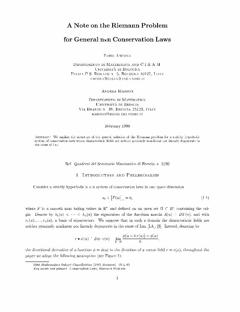
ANote on the Riemann Problemfor General nn Conservation LawsFabio AnconaDipartimento di Matematica and C.I.R.A.M.Universita di BolognaPiazza P.S. Donato n. 5, Bologna 40127, Italyancona@ciram3.ing.unibo.itAndrea MarsonDipartimento di MatematicaUniversita di BresciaVia Branze n. 38, Brescia 25123, Italymarson@bsing.ing.unibs.itFebruary 1999Abstract. We analize the structure of the general solution of the Riemann problem for a striclty hyperbolicsystem of conservation laws whose characteristic elds are neither genuinely non-linear nor linearly degenerate inthe sense of Lax. Ref. Quaderni del Seminario Matematico di Brescia, n. 9/991. Introduction and PreliminariesConsider a strictly hyperbolic n n system of conservation laws in one space dimensionut + F (u)x = 0; (1.1)where F is a smooth map taking values in Rn and dened on an open set Rn containing the ori-gin. Denote by 1(u) < < n(u) the eigenvalues of the Jacobian matrix A(u) := DF (u); and withr1(u); : : : ; rn(u); a basis of eigenvectors. We suppose that in such a domain the characteristic elds areneither genuinely nonlinear nor linearly degenerate in the sense of Lax [LA], [S]. Instead, denoting byr (u) := D r(u) = limh!0 u+ h r(u) (u)h :the directional derivative of a function = (u) in the direction of a vector eld r = r(u), throughout thepaper we adopt the following assumption (see Figure 1):1980 Mathematics Subject Classication (1985 Revision). 35 L 65.Key words and phrases. Conservation Laws, Riemann Problem.1

2 F. Ancona and A. Marson(A) There exist n smooth n1-dimensional manifolds 0i , i = 1; : : : ; n, such that0i := fu 2 ; ri i(u) = 0 g; (1.2)ri ri i u0 6= 0; 8 u0 2 0i : (1.3)

ri

λ iri >0.λ i <0.r

i

u0

R ( )i

Ω 0i

u0.

Figure 1Systems of conservations laws which are neither genuinely non-linear nor linearly degenerate arise inseveral contexts, in particular in studying elastodynamic or rigid heat conductors at low temperature.The purpose of this note is to analyze the structure of the general solution of the Riemann problemassociated with (1.1), i.e. of the Cauchy problem (1.1) with arbitrary initial datau(0; x) = uL if x < 0,uR if x > 0. (1.4)The Riemann Problem plays a key role in the theory of hyperbolic systems of conservation laws. In fact, thesolution of the Riemann problem represents the basic building block towards the construction of solutionsto the general Cauchy Problem for (1.1).We recall that, for hyperbolic systems of conservation laws, to achieve uniqueness of solutions it isnecessary to consider weak solutions that satisfy some additional admissibility condition, possibly motivatedby physical considerations. In [LI1], [LI2], T.P. Liu proposed an admissibility criterion valid for nn systemsof conservation laws having the property that, for each characteristic speed i; the directional derivative riivanishes on a nite, disjoin union of n1-dimensional manifolds. This criterion, in the case of a systemwhere ri i = 0 on a single hypersurface in the u-space, is equivalent to the stability condition introducedby Lax:

A Note on the Riemann Problem 3(L) A shock connecting the left state uL and the right state uR; travelling with speed s is an admissiblediscontinuity of the i-th family if i(uL) s i(uR):In this setting, an entropy weak solution of (1.1) will be a weak solution of (1.1) that has admissible discon-tinuities in the sense of Lax. The existence of a unique, self-similar, entropy weak solution of the Riemannproblem (1.1), (1.4), was established by T.P. Liu in [LI1], [LI2]. Such solution consists of elementarywaves that can be compressive shocks, centered rarefactions or composed waves made of one-side contact-discontinuities adjacent to rarefaction waves.For each characteristic family, one can dene an elementary curve that characterizes the set of all leftand right states uL; uR; which are connected by means of an elementary wave of that family. In this note,in particular, we shall derive some basic properties of the elementary curves associated to each characteristicfamily.Here, we make some standard assumptions and introduce some basic notations. We choose right andleft eigenvectors ri(u); li(u) of A(u) normalized so thatri(u) = 1; (1.5)hli(u); rj(u)i = 1 if i = j0 if i 6= j. (1.6)For any xed u0 2 ; and i = 1; : : : ; n; as usual we dene the i-th rarefaction curve s 7! Riu0)(s)as the integral curve of ri through u0; parametrized by arc-length. We shall often use also the nota-tion exp sri(u0) := Riu0)(s): Moreover, by the implicit function theorem one can dene the i-th shockcurve Si(u0) as the set of points u such thathlj(u; u0); u u0i = 0 8j 6= i; (1.7)where lj(u; u0) is the j-th left eigenvector of the averaged matrixA(u; u0) = Z 10 Au0 + (u0 u)dnormalized as in (1.6). We parametrize also the curve s 7! Si(u0)(s) by arc-length.It is well known [S] that the two curves Ri(u0); Si(u0) have second order tangency at s = 0: Thus thefollowing hold ddsSi(u0)(s)s=0 = riu0; (1.8)d2ds2Si(u0)(s)s=0 = ri riu0: (1.9)The speed of the shock wave connecting the left state uL to the right state Si(uL)(s) = uR is denotedsi u0; s or iuL; uR and satises si uL; 0 = iuL; (1.10)ddssi uL; ss=0 = 12ri iuL: (1.11)

4 F. Ancona and A. MarsonWe shall focus our attention, in particular, on the Riemann problem with constant states uL, uR in (1.4)satisfying rk kuL rk kuR < 0; (1.12)for some k 2 f1; : : : ; ng, i.e. on the case in which the left state uL and the right state uR lie on oppositesides w.r.t. the hypersurface 0k. In this case, by the analysis in [LI1], [LI3], the solution of the Riemannproblem (1.1), (1.4) contains a composed wave of the k-th characteristic family that consists ofCase 1: a rarefaction wave followed by a left contact discontinuity both of the k-th family, ifrk rk ku0 < 0; 8 u0 2 0k; (1.13)i.e. if, for each u0 2 0k; the function s 7! k(exp srk)u0 attains its maximum value at s = 0;Case 2: a right contact discontinuity followed by a rarefaction wave both of the k-th family, ifrk rk ku0 > 0; 8 u0 2 k0 ; (1.14)i.e. if, for each u0 2 0k; the function s 7! k(exp srk)u0 attains its minimum value at s = 0.To take advantage of the symmetry of the system, we shall express the general solution of the Riemannproblem in terms of two types of elementary curves:1. If Case 1 holds, then we construct the elementary curve of right states of the k-th family, that consists ofall right states that are connected with a given left state by an elementary wave of the k-th characteristicfamily.2. If Case 2 holds, then we construct the elementary curve of left states of the k-th family, that consists ofall left states that are connected with a given right state by an elementary wave of the k-th characteristicfamily.In particular, this means that, if Case 1 holds, for any xed u0 2 0k we dene a mixed curve of right statesof the k-th family, denoted s 7! Tku0)(s; having the propertyM1. For every point uR 2 Tk(u0); there exists a unique point uL 2 Rk(u0) such that uR 2 Sk(uL) andk(uL; uR) = k(uL):Instead, if Case 2 holds, for any xed u0 2 0k we dene a mixed curve of left states of the k-th family, stilldenoted s 7! Tku0)(s, having the propertyM2. For every point uL 2 Tk(u0); there exists a unique point uR 2 Rk(u0) such that uR 2 Sk(uL) andk(uL; uR) = k(uR):Throughout, for a one-parameter map s 7! (s); s 2 I R; we shall often use a dot to denote thedierentiation of w.r.t. s: 2. The Mixed CurvesIn this section we want to study the properties of the mixed curves of a xed k-th characteristic family,k 2 f1; : : : ; ng. For sake of simplicity, we assume that (1.13) holds, the other case being entirely similarbecause of the above denitions.

A Note on the Riemann Problem 5Given a point u0 2 0k; i.e. such that rk ku0 = 0, the curve of states in a neighborhood of u0which can be connected to the left by a composed wave made of a rarefaction followed by a left contactdiscontinuity of the k-th characteristic family can be determined by solving the equationF (u) F (exp s rk)(u0) = k(exp s rk)(u0) u (exp s rk)(u0) (2.1)in terms of (s; u) 2 R . Notice that (2.1) implies that the point u = uR lies on the shock curve trough(exp s rk)u0 = uL and that the speed of the shock wave connecting (exp s rk)(u0) with u is preciselyk(exp s rk)(u0): Therefore the vector equation (2.1) is equivalent to the scalar equationsk(exp s rk)(u0); t = k(exp s rk)(u0): (2.2)Indeed, (s; t) is a solution of (2.2) i s; Sk(exp s rk)(u0); t is a solution of (2.1). Clearly a trivial solutionof (2.2) is (s; t) = (s; 0): A non-trivial solution of (2.2) will be determined by rst nding a curve of solutionsof the equation @@tsk(exp s rk)(u0); t = 0 (2.3)and then using such a curve to determine an approximate solution of (2.2) which in turn allows to determinethe exact solution of (2.2) by applying the Newton-Kantorovich Theorem [De]. The main result of this noteis the followingTheorem 2.1. Let k 2 f1; : : : ; ng be such that (1.13) holds. Then for any u0 2 0k; there exists a smoothcurve T := T (u0) = Tk(u0) : s 7! T (u0)(s) 2 , together with two smooth maps := (u0) = k(u0) : s 7!(u0)(s) 2 R; := (u0) = k(u0) : s 7! (u0)(s) 2 R; dened in a neighborhood of zero J , such thatF T (s) F(exp (s) rk)(u0) = k(exp (s) rk)(u0) T (s) (exp (s) rk)u0; (2.4)ddsT (s) = ddtSk (exp (s) rk)u0; t t=(s); (2.5)for all s 2 J : Moreover, the map s 7! (s) + (s) is strictly increasing and, at s = 0; one hasT (0) = u0; (2.6)ddsT (s)s=0 = rku0; (2.7)d2ds2T (s)s=0 = rk rku0: (2.8)Remark 2.1. If we x some k 2 f1; : : : ; ng for which (1.14) holds, then the statement of Theorem 2.1continue to hold, except for the fact that the map s 7! (s) +(s) is strictly decreasing. Towards a proof ofTheorem 2.1, we rst establish two intermediate results.Proposition 2.1. For every u0 2 0k, there exists a unique smooth map := u0 : s 7! u0(s) 2 Rdened in a neighborhood of zero J , such that (0) = 0; (2.9)@@tskh(exp s rk)u0; tit=(s) = 0 8s 2 J : (2.10)

6 F. Ancona and A. MarsonMoreover, one has _(0) = 32 : (2.11)Proof. Since u0 2 0k; by (1.11) we have ddtsku0; tt=0 = 0: (2.12)Then, by dierentiating three times the Rankine-Hugoniot equation as in [LI3] p.8, one obtainsAu0 k(u0) d3dt3Sk(u0)(t)t=0 d2dt2 rkSk(u0)(t)t=0 == 3 d2dt2sku0; tt=0 d2dt2kSk(u0)(t)t=0rk(u0): (2.13)But, the left hand side of (2.13) is proportional to r2u0 and hence we deduce thatd2dt2sku0; tt=0 = 13 d2dt2kSk(u0)(t)t=0: (2.14)Thus, since d2dt2kSk(u0)(t)t=0 = rk rk ku0; (2.15)from (2.14) and because of (1.11) it follows that@2@t2sk(exp s rk)u0; t(s;t)=(0;0) = d2dt2sku0; tt=0 6= 0: (2.16)Therefore, by the implicit function theorem, (2.3) admits a unique smooth solution : s 7! (s) in aneighborhood of zero and by (1.11), (2.14), we nd_(0) = @2@s@tsk(exp s rk)u0; t(s;t)=(0;0)@2@t2sk(exp s rk)u0; t(s;t)=(0;0) = rk rk ku02 d2dt2 sku0; tt=0 = 32 : Proposition 2.2. For every u0 2 0k; there exists a unique smooth map := u0 : s 7! u0(s) 2 Rdened in a neighborhood of zero J , such that (s) 6= 0 whenever s 6= 0, and(0) = 0; (2.17)k(exp s rk)u0 = skh(exp s rk)u0; (s)i 8s 2 J : (2.18)Proof. For any xed u0 2 0k; and s 2 R, consider the mapt 7! Gs(t) := k(exp s rk)u0 skh(exp s rk)u0; ti: (2.19)Then (s) is precisely the non trivial solution ofGs(t) = 0: (2.20)

A Note on the Riemann Problem 7Let be the map dened by Proposition 2.1 and consider the map s 7! ~(s) dened by~(s) = (s)+2k(exp s rk)u0 2kSk(exp s rk)u0; (s) 12 d2dt2 sk(exp s rk)u0; tt=(s) 12;if s 0;~(s) = (s)2k(exp s rk)u0 2kSk(exp s rk)u0; (s) 12 d2dt2 sk(exp s rk)u0; tt=(s) 12;if s > 0:We will show that ~(s) is an approximate solution of (2.20) in the sense thatGs(~(s)) = o(s2); ddtGs(t)t=~(s) = c s+ o(s); (2.21)where o(s); o(s2); are the usual Landau symbols and c 6= 0 a suitable constant. This is sucient to establishthe Proposition which then follows by applying the Newton-Kantorovich Theorem [De]. To prove (2.21) rstobserve that, since satises (2.10) and hencesk (exp s rk)u0; (s) = k Sk(exp s rk)u0; (s) ;it follows thatk (exp s rk)u0 = kSk(exp s rk)(u0)(s)+ 12 d2dt2 sk (exp s rk)u0; t t=(s)((s))2 + o(2(s)):(2.22)Therefore, by using (2.11) and observing that by construction s 7! d2dt2 sk (exp s rk)u0; t t=(s) isbounded away from zero in a neighborhood of zero, we deduce that~(s) = 2(s) + o((s)) = 3s+ o(s); (2.23)and thatGs(~(s)) = kSk(exp s rk)(u0)(s)+ 12 d2dt2sk (exp s rk)u0; t t=(s)(~(s) (s))2 sk (exp s rk)u0; ~(s) == o((~(s) (s))2) = o(s2); (2.24)ddtGs(t)t=~(s) = d2dt2sk (exp s rk)u0; t t=(s)(~(s) (s)) + o((~(s) (s)) == 32 d2dt2sk (exp s rk)u0; t t=(s) s+ o(s): (2.25)

8 F. Ancona and A. MarsonProof of Theorem 2.1 Let be the map dened by Proposition 2.2 and the identity. Then, by (2.17),(2.18), the curve T (s) := Sk(exp (s) rk)(u0)(s) (2.26)satises (2.4), (2.6). Regarding (2.5), (2.7) and (2.8), rst riparametrize by its arclength the curve denedby (2.26) and use ; ; T; to denote the corresponding riparametrized maps as well. Then observe that sinceT (s) belongs to the shock curve through !(s) := (exp (s) rk)u0, dierentiating twice the Rankine-Hugoniotcondition and setting_k(s) := ddt sk!(s); tt=(s); _Sk(s) := ddtSk!(s)(t)t=(s); _T (s) := ddsT (s);k(s) := d2dt2 sk!(s); tt=(s); Sk(s) := d2dt2Sk!(s)(t)t=(s); T (s) := d2ds2T (s);we have DF (T (s)) k (!(s)) _Sk(s) = _k(s)T (s) !(s) (2.27)andDF T (s) k(!(s)) Sk(s) = k(s)T (s) !(s)+ 2 _k(s) _Sk(s)D2F T (s) _Sk(s) _Sk(s): (2.28)On the other hand, dierentiating twice (2.4) w.r.t s; one ndsDF (T (s)) k (!(s)) _T (s) = _(s)DF (!(s)) k (!(s)) rk(!(s))++ _(s) rk k!(s)T (s) !(s)= _(s) rk k!(s)T (s) !(s); (2.29)andDF T (s) k(!(s)) T (s) = ( _(s))2 rk rk k!(s)T (s) !(s)+ 2 _(s) rk k!(s) _T (s)D2F T (s) _T (s) _T (s) ( _(s))2 rk k!(s) rk!(s): (2.30)By comparing (2.27) and (2.29), we deriveDF (T (s)) k (!(s)) _T (s) _(s) rk k!(s)_k(s) _Sk(s)! = 0 8 s: (2.31)Since k(!(s)) > k(T (s)) for all s 6= 0; and since j _Sk(s)j = j _T (s)j 1; from (2.31) we recover (2.5) in thecase s 6= 0. By continuity, (2.5) still holds if s = 0 and hence, recalling that _Sk(0) = rku; we derive (2.7).Finally, using (2.7) and evaluating (2.28), (2.30) at s = 0; we obtainDF u0 ku0 T (0) Sk(0) = 0which, recalling that Sk(0) = Drk rku0; yields (2.8). To conclude the proof we only need to observe that,dierentiating (2.26) at s = 0 one nds _T (0) = _(0) + _(0)rku0; which by (2.7) implies _(0) + _(0) = 1:Hence the map s 7! (s) + (s) is strictly increasing in a neighborhood of zero.

A Note on the Riemann Problem 9Remark 2.2. Since by Theorem 2.1 the map s 7! k(u0)(s) + k(u0)(s); u0 2 0k; is strictly increasing, wecan riparametrize the map s 7! Tk(u0)(s) = SkRk(u0)k(u0)(s)k(u0)(s) (2.32)as 7! Tku0&k(u0)1(); &k(u0) := k(u0) + k(u0): (2.33)Thus, using still k; k; Tk to denote the riparametrized maps, we can write the mixed curve in the formTk(u0)() = SkRk(u0) k(u0)()k(u0)(): (2.34)Notice that, in the new parametrization one has k(u0)() = k(u0)(): On the other hand, by construc-tion, there holds d=d k(u0)() < 0 for all ; which, in turn, impliesddk(u0)() > 1 8 : (2.35)3. The Elementary CurvesThrough each point u 2 ; we construct now the n elementary curves, one for each characteristicfamily, that are used to dene the general entropy-admissible solution of the Riemann problem (1.1), (1.4).As observed in the introduction, we shall construct, alternatively, the elementary curve of right states, or theelementary curve of left states of the k-th characteristic family, depending on which inequality holds between(1.13) and (1.14).First we need some more notations. For each i = 1; : : : ; n, we introduce two mapsi) i : ! R, implicitly dened by Ri(u) i(u) 2 0i ; (3.1)ii) i : ! 0i , dened by i(u) := Ri(u) i(u): (3.2)Recalling the denition (1.2), one clearly hasri ii(u) = 0 8 u 2 : (3.3)By construction, the maps i, i; i = 1; : : : ; n are smooth. From (2.35) it follows that, for any i = 1; : : : ; n;the map 7! i(u0)(s) := s i(u0)(s) is strictly decreasing. Denote 7! 1i (u0)() the inverse map ofs 7! iu0)(s); and set i(u) := ii(u)h1i i(u)i(u)i; u 2 : (3.4)Notice that, since 1i i(u)i(u) = i(u) + i(u)one has Rii(u)hii(u)i(u) + i(u)i = u:

10 F. Ancona and A. MarsonThus, from (2.34) we deduceTii(u)hi(u) + i(u)i = Si(u)hii(u)i(u) + i(u)i = Si(v)i(u): (3.5)Call +i := fu 2 : ri i(u) > 0gi := fu 2 : ri i(u) < 0g i = 1; : : : ; n: (3.6)Fix u 2 ; k 2 f1; : : : ; ng; and let J be the neighborhood of zero at Theorem 2.1. Then, dene theelementary curve of the k-th characteristic family through u; k(u) : J ! ; as follows:1. If (1.13) holds, thenk(u)(s) =

8>>>>>>>>>>>>>>>>>><>>>>>>>>>>>>>>>>>>:Sk(u)(s) 8 s if u 2 0k,8>>><>>>: Sk(u)(s) if s < 0Rk(u)(s) if 0 s k(u)Tkk(u)s+ k(u) if k(u) < s k(u)Sk(u; s) if s > k(u) if u 2 +k ,8>>><>>>: Sk(u)(s) if s > 0Rk(u; s) if k(u) s 0Tkk(u)s+ k(u) if k(u) s < k(u)Sk(u)(s) if s < k(u) if u 2 k . (3.7)

2. If (1.14) holds, thenk(u)(s) =

8>>>>>>>>>>>>>>>>>><>>>>>>>>>>>>>>>>>>:Sk(u)(s) 8 s if u 2 0k,8>>><>>>: Sk(u)(s) if s > 0Rk(u)(s) if k(u) s 0Tkk(u)s+ k(u) if k(u) s < k(u)Sk(u; s) if s < k(u) if u 2 +k ,8>>><>>>: Sk(u)(s) if s < 0Rk(u)(s) if 0 s k(u)Tkk(u)s+ k(u) if k(u) < s k(u)Sk(u)(s) if s > k(u) if u 2 k . (3.8)

Notice that (1.8), (2.5), (2.7) and (3.5) together, imply that, for any xed u 2 ; k 2 f1; : : : ; ng;the map s 7! k(u)(s) is everywhere continuously dierentiable. Thus, by the implicit function theorem,given uL; uR 2 , we can uniquely determine intermediate states uL = !0; !1; : : : ; !n = uR and wave sizes1; : : : ; n 2 J ; such that there holds!k = k(!k1)(k) if (1:13) occurs,!k1 = k(!k)(k) if (1:14) occurs: (3.9)Then the solution to the Riemann Problem with initial data (1.4) can be constructed by piecing togetherthe solutions to the Riemann problems with initial datauk(x) = uk(0; x) = !k1 if x < 0,!k if x < 0, k = 1; : : : ; n: (3.10)

A Note on the Riemann Problem 11The solution to each Riemann problem with initial data uk; k = 1; : : : ; n, is dened as follows.1. Assume that (1.13) holds. There are 3 possibilities:1) !k1 2 0k: the solution consists of a compressive shock of the k-th characteristic family travelling withspeed sk!k1; k:2) !k1 2 +k : the solution consists ofa) 0 k k(!k1): a rarefaction wave of the k-th characteristic family, with characteristic speedsranging over the interval k(!k1); k(!k);b) k < 0 or k k(!k1): a compressive shock of the k-th characteristic family travelling withspeed sk!k1; k;c)k(!k1) < k < k(!k1): a composed wave of the k-th characteristic family made of a a rarefactionwave of size ek := k kk(!k1); k + k(!k1);with characteristic speeds ranging over the intervalk(!k1); k(e!k1); e!k1 := Rk!k1; ek;followed by a left-contact discontinuity bk := k ek; travelling with speedske!k1; bk = k(e!k1):3) !k1 2 k : the solution consists ofa) k(!k1) k 0: a rarefaction wave as in 2-a);b) k > 0 or k < i(!k1): a compressive shock as in 2-b);c) k(!k1) < k < k(!k1): a composed wave as in 2-c), made of a rarefaction wave followed bya left-contact discontinuity.2. Assume that (1.14) holds. There are 3 possibilities:1) !k 2 0k: the solution consists of a compressive shock of the k-th characteristic family travelling withspeed sk!k; k:2) !k 2 +k : the solution consists ofa) k(!k) k 0: a rarefaction wave of the k-th characteristic family, with characteristic speedsranging over the interval k(!k1); k(!k);b) k > 0 or k < k(!k): a compressive shock of the k-th characteristic family travelling withspeed sk!k; k;c) k(!k) < k < k(!k): a composed wave of the k-th characteristic family made of a right-contactdiscontinuity of size bk := kk(!k); k + k(!k);

12 F. Ancona and A. Marsontravelling with speed ske!k; bk = k(e!k); e!k := Rk!k; k bk;followed by a rarefaction wave of size ek := k bk; with characteristic speeds ranging over theinterval k(e!k); k(!k):3) !k 2 k : the solution consists ofa) 0 k k(!k): a rarefaction wave as in 2-a);b) k < 0 or k k(!k): a compressive shock as in 2-b);c) k(!k) < k < k(!k): a composed wave as in 2-c), made of a right-contact discontinuity followedby a rarefaction wave.Acknowledgments This research was partially supported by TMR project HCL ERBFMRXCT360033.References[Da] C.M. Dafermos, Regularity and large time behaviour of solutions of a conservation law withoutconvexity, Proc. Royal Soc. Edinburgh. , 99 A (1985), pp. 201-239.[De] K. Deimling, Nonlinear Functional Analysis, Springer-Verlag, 1985.[LA] P.D. Lax, Hyperbolic Systems of Conservation Laws II, Comm. on Pure and Applied Math., 10 (1957),pp. 537-566.[LI1] T.P. Liu, The Riemann problem for general 2 2 conservation laws, Trans. Amer. Math. Soc., 199(1974), pp. 89-112.[LI2] T.P. Liu, The Riemann problem for general systems of conservation laws, J. Dierential Equations, 18(1975), pp. 218-234.[LI3] T.P. Liu, Admissible solutions of hyperbolic conservation laws, Memoir Amer. Math. Soc., 30 (1981),no. 240.[S] J. Smoller, Shock Waves and Reaction-Diusion Equations, Second Edition, Springer-Verlag, 1994.