A Wavefront Tracking Algorithm for N×N Nongenuinely Nonlinear Conservation Laws

454

⁄0022-0396/01 $35.00© 2001 Elsevier ScienceAll rights reserved.

Journal of Differential Equations 177, 454–493 (2001)doi:10.1006/jdeq.2000.4012, available online at http://www.idealibrary.com on

A Wavefront Tracking Algorithm for N×N NongenuinelyNonlinear Conservation Laws1

1 This work has been partially supported by TMR Project HCL ERBFMRXCT960033.

Fabio Ancona

Dipartimento di Matematica and C.I.R.A.M., Università degli Studi di Bologna,P.zza Porta S. Donato 5, 40123 Bologna, Italy

E-mail: [email protected]

and

Andrea Marson

Dipartimento di Matematica, Università di Brescia, Via Valotti 9, 25133 Brescia, ItalyE-mail: [email protected]

Received July 20, 2000

We introduce a wavefront tracking algorithm for N×N hyperbolic systems ofconservation laws

ut+F(u)x=0,

that admits characteristic fields that are neither genuinely nonlinear nor linearlydegenerate in the sense of Lax. Instead we assume that, for any nongenuinely non-linear ith characteristic family, the derivative of the ith eigenvalue li(u) of DF(u)in the direction of the ith right eigenvector ri(u), vanishes on a single (N−1)-dimensional hypersurface in the u-space, transversal to the field ri(u). Systems thatfulfill this type of assumptions are of particular interest in studying elastodynamic orrigid heat conductors at low temperature. The first proof of the existence of weaksolutions for nongenuinely nonlinear systems was given by T. P. Liu (Mem. Amer.Math. Soc. 30 (1981), no. 240), based on a Glimm scheme. Our construction hereprovides an alternative method for establishing the global existence of weak solutionsfor such systems. Moreover, relying on the stability analysis developed in Ancona andMarson, preprint S.I.S.S.A.-I.S.A.S. 27/99/11, 1999, and preprint, 2000, we showthat these solutions are entropy admissible in the sense of Lax. © 2001 Elsevier Science

Key Words: hyperbolic systems; conservation laws; nongenuinely nonlinearity;front tracking approximations.

1. INTRODUCTION

Consider the Cauchy problem for an N×N strictly hyperbolic system ofconservation laws

ut+F(u)x=0=0 (1.1)

u(0, x)=u(x). (1.2)

Here, t \ 0 and x ¥ R are, respectively, the time and the space variable,while the vector u=u(t, x) ¥ RN represents the conserved quantities. Theflux function F is assumed to be a smooth vector field defined on a neigh-borhood of the origin W ı RN and taking values in RN. Denote withl1(u) < · · · < lN(u) the eigenvalues of the Jacobian matrix DF(u), and withr1(u), ..., rN(u) a corresponding basis of eigenvectors. We assume thatsystem (1.1) admits nongenuinely nonlinear (NGNL) characteristic fields, i.e.characteristic fields that are neither genuinely nonlinear (GNL) nor linearlydegenerate (LD) in the sense of Lax [La, Sm]. Instead, we require that, foreach NGNL characteristic field rk, the directional derivative of lk in thedirection of rk

Drk lk(u) q limh Q 0

lk(u+hrk(u))− lk(u)h

vanishes on a smooth hypersurface transversal to the field rk. Moreprecisely, we make the following assumption (see Fig. 1):

(A) If the kth characteristic family is NGNL, then there exists an(N−1)-dimensional smooth manifold W0

k, k=1, ..., N, such that

W0k={u ¥ W : Drk lk(u)=0}, (1.3)

D2rk lk(u) q Drk (Drk lk)(u) ] 0, -u ¥ W0

k. (1.4)

Systems of conservation laws with characteristic fields that fulfill theassumption (A) physically arise in several contexts, for instance in studyingelastodynamic (e.g., see [Dp2]) or rigid heat conductors at low tempera-ture [RMS1, RMS2]. An example is given by the generalized Cattaneomodel proposed by T. Ruggeri and co-workers [RMS1, RMS2] to describethe heat propagation in high-purity crystals (He, NaF, Bi):

[re]t+qx=0, [aq]t+nx=−nŒ

oq. (1.5)

A WAVEFRONT TRACKING ALGORITHM 455

FIG. 1. Assumption (A).

Here r denotes the constant mass density, q=q(t, x) the one-dimensionalheat flux, e=e(h) the internal energy depending on the absolute tempera-ture h=h(t, x), while a=a(h) and n=n(h) are constitutive scalar func-tions (depending on the material), nŒ is the derivative of n with respect to h,and o=o(h) is the heat conductivity. Equation (1.5)1 represents the energybalance, while (1.5)2 is a generalization of the Maxwell–Cattaneo equation.In the range of temperature in which one can observe the so-called ‘‘secondsound’’ effect, the heat conductivity becomes very high and thus the sys-tem (1.5) can be assumed to be homogeneous. A direct computation of thecorresponding characteristic speeds shows that such a system shares theproperty (A).

It is well known that, because of the nonlinear dependence of the char-acteristic speeds lk(u) on the state variable u, systems of conservation laws,in general, do not admit smooth solutions globally defined in time. There-fore, weak solutions in the sense of distributions are considered. We recallthat a continuous map t W u(t, · ), with values in L1

loc(R; RN), is a weaksolution to the Cauchy problem (1.1)–(1.2) if the initial condition (1.2) isverified and, for any smooth function f with compact support contained in(0, +.)×R, there holds

F.

0F.

−.[u(t, x) ft(t, x)+F(u(t, x)) fx(t, x)] dx dt=0. (1.6)

Since, in general, weak solutions to (1.1)–(1.2) are not unique, an entropycriterion for admissibility is usually added to rule out nonphysical discon-tinuities. In [Li1, Li2] T. P. Liu proposed an admissibility criterion validfor general systems of conservation laws with NGNL characteristic fields.In the case of systems satisfying the assumption (A), this criterion isequivalent to the classical stability condition introduced by Lax [La, Sm](cfr. Def. 3.1).

456 ANCONA AND MARSON

For general N×N systems of the type considered in [Li2] the existenceof global weak solutions to (1.1)–(1.2), with small total variation, was firstobtained in [Li3], using the Glimm scheme. An alternative method forconstructing solutions of the Cauchy problem, as limit of a sequence ofpiecewise constant approximate solutions defined by a front tracking algo-rithm, is developed in [AM2, AM3] for systems of two equations in whichboth characteristic families satisfy the assumption (A).

The main goal of the present paper is to extend the result in [AM2,AM3] providing a front tracking algorithm valid for N×N systems withNGNL characteristic fields that satisfy the assumption (A). We remarkthat the construction of weak solutions of (1.1) obtained as limit of asequence of front tracking approximations, together with the L1-stabilityanalysis developed in [AM3, AM5], is fundamental to establish the well-posedness theory for the Cauchy problem (1.1)–(1.2). Indeed, the L1-stability estimates obtained in [AM3, AM5] imply that any sequence offront tracking approximate solutions of (1.1)–(1.2) converges to a uniquelimit u=u(t, x), and that the resulting map (u, t) W St u q u(t, · ) defines auniformly Lipschitz continuous semigroup, whose trajectories are weaksolutions to (1.1). Relying on these results, and using the same technique in[B3], we show here that a Lipschitz continuous semigroup of solutions to(1.1), compatible with the standard solutions of the Riemann problem, isnecessarily unique (up to the domain) and that the trajectories of such asemigroup are entropy weak solutions of (1.1) in the sense of Lax. One canthen obtain the well-posedness theory with similar arguments as in [B-G,B-L], showing that any entropy weak solution to (1.1)–(1.2) must coincidewith the trajectory of the semigroup, provided that the total variation ofthe solution does not grow too wildly.

The basic ideas involved in the construction of piecewise constantapproximate solutions, based on wave-front tracking, were introduced inthe papers of Dafermos [Da] for scalar equations and DiPerna [Dp1] for2×2 systems, then extended in [B1, R, BJ] to general N×N systems withGNL or LD characteristic fields. The construction starts at time t=0 bytaking a piecewise constant approximation u(0, x) of the initial data u(x).At each point of discontinuity of u the resulting Riemann problems arethen solved within the class of piecewise constant functions by using anapproximate Riemann solver that replace centered rarefaction waves withrarefaction fans containing several small jumps traveling with a speed closeto the characteristic speed. Next, one tracks the outgoing fronts until thefirst time two waves interact. The corresponding Riemann problems can besolved applying again the approximate Riemann solver, etc. The mainsource of technical difficulty in this construction stems from the fact thatthe number of lines of discontinuity may approach infinity in finite time.To overcome such a difficulty, the algorithms in [B1, BJ] adopt two


different procedures for approximate solving a Riemann problem withinthe class of piecewise constant functions: an Accurate Riemann Solver,which introduces several new wavefronts, and a Simplified Riemann Solver,which involves a minimum number of outgoing wavefronts and collect allthe remaining new waves into a single nonphysical front, traveling with aspeed strictly larger than all characteristic speeds. This second procedure isused whenever the product of the strengths of the incoming waves becomessmaller than a threshold parameter r, so to generate a new nonphysicalfront with very small amplitude.

Unfortunately, in the case of NGNL systems, this algorithm fails toprevent the number of wave-fronts from approaching infinity within afinite time. This is the consequence of the different structure for suchsystems of the elementary waves contained in the exact solution of theRiemann Problem. In fact, in contrast with the standard GNL systems, thesolution of a Riemann problem for NGNL systems may contain composedwaves made of several contact discontinuities separated by centered rare-faction waves (see [Li2]). In particular, for systems satisfying the assump-tion (A), the general self-similar solution of a Riemann problem consists ofrarefaction waves, compressive shocks and composed waves made of asingle one-sided contact-discontinuity adjacent to a rarefaction wave[AM1]. The presence of such composed waves in the solution of theSimplified Riemann Solver can possibly determine a blow-up of thenumber of wavefronts.

We thus need to modify the algorithm by introducing two different typesof Simplified Riemann Solvers. If e is the small parameter that controls themaximum strength of the rarefaction fronts generated by the AccurateRiemann Solver, and if the exact solution of the Riemann problem con-tains rarefaction waves of strength greater than 3e, then we basically definethe approximate solution of the Riemann problem with the same procedureas for the Simplified Riemann Solvers in [B1, BJ]. In the case where thestrength of an outgoing rarefaction wave is smaller than the thresholdparameter 3e, we lump together all new fronts of the outgoing (possiblycomposed) wave that contains the rarefaction into a single wavefront. Inboth cases we still collect the remaining new waves into a single nonphysi-cal front as in [B1, BJ]. This procedure allows to keep finite the totalnumber of wave-fronts for any time t > 0.

A key part of the proof of the global existence of approximate solutionsgenerated by wavefront tracking consists in deriving a-priori bounds on thetotal variation. As customary, these a priori estimates are obtained using afunctional Q that measures the potential interaction of waves in the solu-tion. In particular, for NGNL systems, T. P. Liu [Li3] introduced a func-tional Q in which the amount of potential interaction between waves of thesame family is proportional to the product of the strengths of the waves


and of the negative part of their angle. This choice is motivated by the factthat no interaction between two waves is expected when their angle is non-negative.

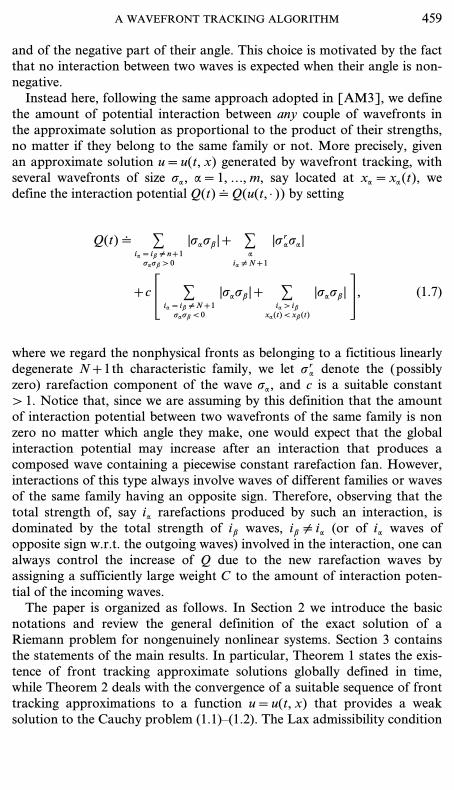
Instead here, following the same approach adopted in [AM3], we definethe amount of potential interaction between any couple of wavefronts inthe approximate solution as proportional to the product of their strengths,no matter if they belong to the same family or not. More precisely, givenan approximate solution u=u(t, x) generated by wavefront tracking, withseveral wavefronts of size sa, a=1, ..., m, say located at xa=xa(t), wedefine the interaction potential Q(t) q Q(u(t, · )) by setting

Q(t) q Cia=ib ] n+1sasb > 0

|sasb |+ Ca

ia ] N+1

|s rasa |

+c r Cia=ib ] N+1sasb < 0

|sasb |+ Cia > ib

xa(t) < xb(t)

|sasb |s , (1.7)

where we regard the nonphysical fronts as belonging to a fictitious linearlydegenerate N+1th characteristic family, we let s r

a denote the (possiblyzero) rarefaction component of the wave sa, and c is a suitable constant> 1. Notice that, since we are assuming by this definition that the amountof interaction potential between two wavefronts of the same family is nonzero no matter which angle they make, one would expect that the globalinteraction potential may increase after an interaction that produces acomposed wave containing a piecewise constant rarefaction fan. However,interactions of this type always involve waves of different families or wavesof the same family having an opposite sign. Therefore, observing that thetotal strength of, say ia rarefactions produced by such an interaction, isdominated by the total strength of ib waves, ib ] ia (or of ia waves ofopposite sign w.r.t. the outgoing waves) involved in the interaction, one canalways control the increase of Q due to the new rarefaction waves byassigning a sufficiently large weight C to the amount of interaction poten-tial of the incoming waves.

The paper is organized as follows. In Section 2 we introduce the basicnotations and review the general definition of the exact solution of aRiemann problem for nongenuinely nonlinear systems. Section 3 containsthe statements of the main results. In particular, Theorem 1 states the exis-tence of front tracking approximate solutions globally defined in time,while Theorem 2 deals with the convergence of a suitable sequence of fronttracking approximations to a function u=u(t, x) that provides a weaksolution to the Cauchy problem (1.1)–(1.2). The Lax admissibility condition


for the weak solution follows from Theorem 3 which also states theuniqueness of a Lipschitz continuous semigroup of solutions to (1.1),compatible with the Lax admissible solutions of the Riemann problem.Section 3 contains the proofs of Theorem 2–3, while the proof ofTheorem 1 is given in Section 5. The wavefront tracking algorithm isdescribed in Section 4.

2. PRELIMINARIES

Since the system at (1.1) is supposed to be strictly hyperbolic andbecause we will consider only solutions with small total variation, we shallassume throughout the paper that there exists a positive constant l suchthat

|lk(u)| < l, -u ¥ W, k=1, ..., N. (2.1)

For any fixed u0 ¥ W, and k=1, ..., N, let

s W Rk(u0)[s], s W Sk(u0)[s], (2.2)

denote, respectively, the k-rarefaction and the k-shock curve throughu0 ¥ W. Without loss of generality, by possibly performing a linear changeof coordinates, we may assume that the kth component uk of the vectoru ¥ Rk(u0) (u ¥ Sk(u0)) is strictly monotone along Rk(u0) (Sk(u0)). Thus, asin [Li3], we choose the parameter s in (2.2) so that

(Rk(u0)[s])k=(Sk(u0)[s])k=u0k+s. (2.3)

This, in particular, means that the strength of a k-wave (uL, uR) will bedefined as

|(uL, uR)| q |uLk −uRk |, (2.4)

where uLk , uRk denote, respectively, the kth component of the left state uL

and of the right state uR. Recalling that, using a suitable parameterization,the shock curve Sk(u0)[ · ] and the rarefaction curve Rk(u0)[ · ] have asecond-order contact at their initial state u0, we may normalize the kthright eigenvector rk(u) of the Jacobian matrix A(u)=DF(u) so that

dds

Sk(u)[s]:s=0

=rk(u). (2.5)


In this way, with the parameterization in (2.3), the two curves Rk(u0)[ · ],Sk(u0)[ · ] have a second-order tangency at s=0. The speed of a shockwave connecting the left state uL to the right state uR=Sk(uL)[s] by thekth eigenvalue l s

k(uL, uR) of the averaged matrix

A(uL, uR) q F1

0A(uR+t(uR−uS)) dt

and will be equivalently denoted l sk(uL)[s].

The general entropy admissible solution of a Riemann problem (uL, uR)for a system with NGNL characteristic fields satisfying the assumption (A)consists of rarefaction waves, compressive shocks and composed wavesmade of one-sided contact-discontinuities adjacent to rarefaction waves(see [Li1, Li2, AM1]). In particular, if the kth characteristic family isNGNL, because of (1.3)–(1.4) a composed wave of the kth characteristicfamily, connecting a left state uL with a right state uR, may appear only inthe case where uL and uR lie on opposite sides with respect to the manifoldW0

k. Such a wave consists of

Case 1. a left contact-discontinuity on the right of a rarefaction wave,both of the kth characteristic family, if

D2rk lk(u0) < 0, u0 ¥ W0

k, (2.6)

i.e., if, for each u ¥ W, the characteristic speed lk attains its maximum valuealong the rarefaction curve Rk(u) at the intersection point Rk(u) 5 W0

k;

Case 2. a right contact-discontinuity on the left of a rarefaction wave,both of the kth characteristic family, if

D2rk lk(u0) > 0, u0 ¥ W0

k, (2.7)

i.e., if, for each u ¥ W, the characteristic speed lk attains its maximum valuealong the rarefaction curve Rk(u) at the intersection point Rk(u) 5 W0

k;

In order to express the general solution of the Riemann problem, to takeadvantage of the symmetry of the system we define for the NGNL charac-teristic families two different types of elementary curves, according towhich of the above two cases occurs (see [AM1]).

If (2.6) holds: we define the elementary curve through u0 of right states ofthe kth characteristic family, that consists of all right states connected withthe left state u0 by an elementary wave (rarefaction, shock or composedwave) of the kth characteristic family.If (2.7) holds: we define the elementary curve through u0 of left states of

the kth characteristic family, that consists of all left states connected with


the right state u0 by an elementary wave (rarefaction, shock or composedwave) of the kth characteristic family.

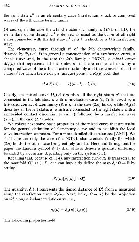
Of course, in the case the kth characteristic family is GNL or LD, theelementary curve through u0 is defined as usual as the curve of all rightstates connected with the left state u0 by a kth shock or a kth rarefactionwave.

The elementary curve through u0 of the kth characteristic family,denoted by Yk(u0), is in general a concatenation of a rarefaction curve, ashock curve and, in the case the kth family is NGNL, a mixed curvesMk(u) that represents all the states u1 that are connected to u by acomposed wave of the kth characteristic family and thus consists of all thestates u1 for which there exists a (unique) point u ¥ Rk(u) such that

u1 ¥ Sk(u), l sk(u, u1)=lk(u). (2.8)

Clearly, the mixed curve Mk(u) describes all the right states u1 that areconnected to the left state u with a rarefaction wave (u, u) followed by aleft-sided contact discontinuity (u, u1), in the case (2.6) holds, while Mk(u)describes all the left states u1 which are connected to the right state u with aright-sided contact discontinuity (u1, u) followed by a rarefaction wave(u, u), in the case (2.7) holds.

We collect next some basic properties of the mixed curve that are usefulfor the general definition of elementary curve and to establish the localwave interaction estimates. For a more detailed discussion see [AM1]. Weshall consider only the case of a NGNL characteristic family for which(2.6) holds, the other case being entirely similar. Here and throughout thepaper the Landau symbol O(1) shall always denote a quantity uniformlybounded by a constant depending only on the system (1.1).

Recalling that, because of (1.4), any rarefaction curve Rk is transversal tothe manifold W0

k at (1.3), one can implicitly define the map dk: W Q R bysetting

Rk(u)[dk(u)] ¥ W0k. (2.9)

The quantity, dk(u) represents the signed distance of W0k from u measured

along the rarefaction curve Rk(u). Next, let pk: W Q W0k be the projection

on W0k along a k-characteristic curve, i.e.,

pk(u)=Rk(u)[dk(u)]. (2.10)

The following properties hold.


1. There exists a smooth map u W nk(u) such that

l sk(u)[nk(u)]=lk(u) -u ¥ W. (2.11)

The quantity nk(u) represents the size of a left-sided contact discontinuityconnecting the left state u with the right state Sk(u)[nk(u)]. The map nk hasthe following expansion

nk(u)=3dk(u)+O(1) |dk(u)|2 -u ¥ W. (2.12)

2. For any fixed u0 ¥ W with Drk lk(u0) > 0, there exists a smooth map

s W zk(u0)[s] s ¥ [dk(u0), nk(u0)], (2.13)

such that

zk(u0)[dk(u0)]=dk(u0), zk(u0)[nk(u0)]=0, (2.14)

lk(Rk(u0)[zk(u0)[s]])=l sk(Rk(u0)[zk(u0)[s]])[s − zk(u0)[s]].

(2.15)

The relation (2.15) says that the left state u0 and the right state

Sk(Rk(u0)[zk(u0)[s]])[s − zk(u0)[s]]

are connected by a composed wave of size s consisting of a rarefactionwave of size zk(u0)[s] followed by a left-sided contact discontinuity of sizes − zk(u0)[s]. The map zk(u0) has the expansion

zk(u0)[s]=(3d r

k(u0)− s)2

+O(1) |s − d rk(u0)|2. (2.16)

3. For any fixed u0 ¥ W, the mixed curve Mk(u0) is given by

Mk(u0)[s]=Sk(Rk(u0)[zk(u0)[s]])[s − zk(u0)[s]]. (2.17)

Moreover, Mk(u0) has a second order tangency at Mk(u0)[dk(u0)] withRk(u0), and has a firs-order tangency at Mk(u0)[nk(u0)] with Sk(u0).

For any NGNL kth characteristic family, consider the sets

W+k q {u ¥ W : Drk lk(u) > 0}, W−

k q {u ¥ W : Drk lk(u) < 0}. (2.18)

Then, in case (2.6) holds, define the elementary curve s Q Yk(u)[s] asfollows


Yk(u)[s]=˛Sk(u)[s] -s if u ¥ W0

k,

˛Sk(u)[s]Rk(u)[s]Mk(u)[s]Sk(u)[s]

if s < 0if 0 [ s [ dk(u)if dk(u) < s [ nk(u)if s > nk(u)

if u ¥ W+k ,

˛Sk(u)[s]Rk(u)[s]Mk(u)[s]Sk(u)[s]

if s > 0if dk(u) [ s [ 0if nk(u) [ s < dk(u)if s < nk(u)

if u ¥ W−k .

(2.19)

Entirely similar definitions are given for Yk(u)[ · ] in the case (2.7) holdsinstead of (2.6). Notice that, whenever a left state uL and a right state uR

are connected by an entropy admissible discontinuity of the kth NGNLfamily, one of the following two cases occurs:

E1. The two states uL, uR lie on the same side w.r.t. the manifold W0k

and

if (2.6) holds, letting s be the size of the corresponding jump, i.e.,uR=Yk(uL)[s], one has

sgn(s) ] sgn(Drk lk(uL));

if (2.7) holds, letting s be the size of the corresponding jump, i.e.,uL=Yk(uR)[s], one has

sgn(s)=sgn(Drk lk(uR)).

E2. The two states uL, uR lie on opposite sides w.r.t. the manifold W0k

and

if (2.6) holds, letting s be the size of the corresponding jump, i.e.,uR=Yk(uL)[s], one has

sgn(s)=sgn(Drk lk(uL)), |s| \ |nk(uL)|; (2.20)

if (2.7) holds, letting s be the size of the corresponding jump, i.e.,uL=Yk(uR)[s], one has

sgn(s) ] sgn(Drk lk(uR)), |s| \ |nk(uR)|. (2.21)

In the case the kth characteristic family is LD or GNL with

Drk lk(u) > 0 -u ¥ W, (2.22)


the corresponding elementary curve is defined as usual by setting

Yk(u)[s]=˛Rk(u)[s] if s \ 0,Sk(u)[s] if s < 0.

(2.23)

Thus, for any uL, uR in a sufficiently small neighborhood of the originWŒ … W, by the Implicit Function Theorem we can uniquely determineintermediate states uL=w0, w1, ..., wN=uR, and wave sizes s1, ..., sN, suchthat there holds

wk=Yk(wk−1)[sk] if (2.6) occurs,

wk−1=Yk(wk)[sk] if (2.7) occurs.(2.24)

Then the solution to the Riemann problem with initial data (uL, uR) can beconstructed by piecing together the solutions to the Riemann problemswith initial data

uk(x)=uk(0, x)=˛wk−1 if x < 0,wk if x < 0,

k=1, ..., N.

If (2.24) holds, we say that wk−1 and wk are connected by a k-wave of sizesk. Throughout the paper, with a slight abuse of notations, we shall simplycall s a wave of size s.

Remark 2.1. Given a wave (uL, uR) of size s, belonging to the kthNGNL family, we will often use a superscript r and a superscript s todenote, respectively, the sizes of its rarefaction and shock components, i.e.

(uL, uR) r q s r q zk(uL)[s], if (2.6) holds,

(uL, uR) r q s r q zk(uR)[s], if (2.7) holds,

(uL, uR) s q s s q s − s r,

(2.25)

where s Q zk(u)[s] denotes the map defined at (2.13)–(2.15).

We collect next the basic estimates on the change of wave-size after aninteraction whose proofs are quite standard and can be derived with thesame arguments in [B2, Section 7], using the implicit function theorem, thegeometrical properties of rarefaction, shock and mixed curves, and theexpansions (2.12), (2.16). Let us give first the following.

Definition 2.1. Given two incoming waves of size sŒ, sœ, we define thequantity of interaction I(sŒ, sœ) between sŒ and sœ as


I(sŒ, sœ) q ˛[|(sŒ+sœ) r − s −r|+|s −s|] |sœ|

if sŒ, sœ belong to the kth NGNLcharacteristic family, sŒsœ > 0and 2.6 holds,

[|(sŒ+sœ) r − s'r|+|s's|] |sŒ|if s, sœ belong to the kth NGNLcharacteristic family, sŒsœ > 0and 2.7 holds,

|sŒsœ| in all the other cases,

(2.26)

where, in the case sŒ, sœ belong to the same kth NGNL characteristicfamily, we interpret sŒ+sœ as the size of a k-wave having the same left(right) state as sŒ (sœ) if (2.6) ((2.7)) holds.

Lemma 2.1. For any compact set K … W, there exists constants C0, C1,m1 > 0, such that, whenever uL, uR ¥ K, |s −i |, |s'i | |s −j | [ m1, the followingstatements hold.

(i) Let s −i, s −j be the sizes of two incoming waves belonging to the dis-tinct characteristic families i > j. Assume that s −i is located on the left of s −j,and that uL, uR are, respectively, the left state of s −i and the right state of s −j.Then, the sizes of the outgoing waves sk, k=1, ..., N, defined at (2.24),satisfy

|si − s −i |+|sj − s −j |+ Ck ] i, j

|sk | [ C1I(s −i, s −j). (2.27)

If si, sj are composed waves and s ri , s r

j are the sizes of their rarefactioncomponents, then there holds

C0 min{|s −j |, |s −i |} [ |s ri − s −ri |, |s r

j − s −rj | [ C1 min{|s −j |, |s −i |}.(2.28)

Moreover, if we consider the auxiliary right state u, connected on the left touL by a j-wave of size s −j followed by an i-wave of size s −i, then one has

|uR−u| [ C1I(s −i, s'j ). (2.29)

(ii) Let s −i, s'i be the sizes of two incoming waves, both belonging to theith characteristic family. As before, assume that s −i is located on the left ofs'i , and that uL, uR are, respectively, the left state of s −i and the right state of


s'i . Then, the sizes of the outgoing waves sk, k=1, ..., N, defined at (2.24),satisfy

|si − s −i − s'i |+Ck ] i

|sk | [ C1I(s −i, s'i ). (2.30)

If si is a composed wave, s ri is the size of its rarefaction component, and

sŒ+sœ represents the size of an i-wave having left state uL, then one has

|s ri −(s −i+s'i ) r| [ C1I(s −i, s'i ). (2.31)

Furthermore, whenever s −i · s'i < 0, there holds

C0 min{|s −i |, |s'i |} [ |s ri − s −ri +s'r

i | [ C1 min{|s −i |, |s'i |}. (2.32)

Moreover, if we consider the auxiliary right state u, connected on the left touL by an i-wave of size s −i+s'i , then one has

|uR−u| [ C1I(s −i, s'i ). (2.33)

(iii) Let (uL, uR), (vL, vR), vL, vR ¥ K, be two i-waves of size s, andassume that |s|, |uL−vL| [ m1. Then one has

|vR−uR|− |vL−uL| [ C1 |s| |vL−uL|. (2.34)

3. STATEMENTS OF MAIN RESULTS

In this section we first present a result that states the existence of fronttracking approximate solutions to (1.1)–(1.2) defined for all time t > 0,whose proof is postponed to Sections 4 and 5. Next, we establish the con-vergence of a suitable sequence of approximate solutions to a limit u=u(t, x) that provides a weak solution of (1.1)–(1.2). Finally, relying on theL1-stability estimates obtained in [AM3, AM5], we show that weak solu-tions of the Cauchy problem constructed as limit of front tracking approx-imations actually satisfy the Lax entropy conditions and generate a uniqueLipschitz continuous semigroup of solutions to (1.1)–(1.2), compatible withthe Lax entropy admissible solutions of the Riemann problem.

Theorem 1. Assume that system (1.1) is strictly hyperbolic and that eachNGNL characteristic family satisfy the assumption (A). Then, there existsd0 > 0 with the following property. For every initial condition u ¥ L1 satisfying

Tot.Var.(u) < d0, (3.1)


and for every e > 0 there exists a uniformly (in e) Lipschitz continuous map

t W ue(t, · ), t ¥ [0,.),

with values in L1loc(R; RN), that provides an e-approximate solution of

(1.1)–(1.2) in the following sense:

1.

||ue(0, · )− u ||L1 < e. (3.2)

2. There exists d > 0 such that

Tot.Var.(ue(t, · )) [ d, -t > 0, e > 0. (3.3)

3. As a function of two variables, ue=ue(t, x) is piecewise constantwith discontinuities occurring along finitely many straight lines in the t-xplane. Only finitely many wavefronts interactions occur, each involvingexactly two incoming fronts. Jumps can be of three types: shocks (or one-sided contact discontinuities), rarefactions and nonphysical waves, denoted,respectively, as S, R, NP. The set of all jumps is denoted J=S 2R 2NP.

4. Along each shock (or contact discontinuity) x=xa(t), a ¥S, thevalues uL q ue(t, xa−) and uR q ue(t, xa+) satisfy one of the followingconditions.

(a) There exists some wave size sa and some index ka ¥ {1, ..., N}corresponding to a NGNL characteristic family for which (2.6) holds, suchthat

|uR−Ska (uL)[sa]|=O(1) · e |sa |. (3.4)

If the states uL, Ska (uL)[sa] lie on the same side w.r.t. the manifold W0

ka , theLax entropy admissibility conditions E1 for (uL, Ska (u

L)[sa] also holds.Otherwise, there holds

sgn(sa)=sgn(Drkalka (u

L)), |sa | \ |nka (uL)| −O(1) · e. (3.5)

(b) There exists some wave size sa and some index ka ¥ {1, ..., N}corresponding to a NGNL characteristic family for which (2.7) holds, suchthat

|uL−Ska (uR)[sa]|=O(1) · e |sa |. (3.6)


If the states Ska (uR)[sa], uR lie on the same side w.r.t. the manifold W0

ka , theLax entropy admissibility conditions E2 for (Ska (u

R)[sa], uR) also holds.Otherwise, there holds

sgn(sa) ] sgn(Drkalka (u

R)), |sa | \ |nka (uR)|−O(1) · e. (3.7)

(c) There exists some wave size sa and some index ka ¥ {1, ..., N}corresponding to a GNL or LD characteristic family, such that

|uR−Ska (uL)[sa]|=O(1) · e |sa |. (3.8)

If the ka th family is GNL, then the Lax entropy admissibility conditionsa < 0 also holds.

Moreover, in any of the above cases, the speed xa of the shock front satisfies

|xa− l ska (u

L, uR)|=O(1) · e. (3.9)

5. Along each rarefaction front x=xa(t), a ¥R, the values uL que(t, xa−) and uR q ue(t, xa+) are related by

uR=Rka (uL)[sa],

for some ka ¥ {1, ..., N} corresponding to a GNL or NGNL characteristicfamily satisfying (2.6), and some wave size sa such that

sa=O(1) · e, sgn(sa)=sgn(Drkalka (u

L)), (3.10)

or by

uL=Rka (uR)[sa],

for some ka ¥ {1, ..., N} corresponding to a NGNL characteristic familysatisfying (2.7), and some wave size sa such that

sa=O(1) · e, sgn(sa) ] sgn(Drkalka (u

L)). (3.11)

Moreover, the speed xa of the rarefaction front satisfies

|xa− lka (uL)|=O(1) · e. (3.12)

6. All nonphysical fronts x=xa(t), a ¥NP have the same speed

xa — l, (3.13)


where l is a fixed constant strictly greater than all characteristic speedslk(u), u ¥ W, k=1, ..., N, i.e.,

l > li(u), -u ¥ W, i=1, ..., N. (3.14)

The total strength of all nonphysical fronts in u(t, · ) remains uniformly small,namely one has

Ca ¥NP

|ue(t, xa+)−ue(t, xa−)|=O(1) · e -t \ 0. (3.15)

The proofs of the next two theorems rely only on the qualitative proper-ties (3.2)–(3.15) of the approximate solutions stated in Theorem 1, and noton the particular front-tracking algorithm used to construct them.

Theorem 2. In the same setting as Theorem 1, assume that the initialcondition u ¥ L1 satisfies (3.1). Let {en}n ¥N be a sequence of positive realnumber converging to zero, and let un q uen (t, x) be an en-approximate solu-tion of (1.1)–(1.2) constructed as in Theorem 1. Then there exists a sub-sequence of {un}n ¥N converging in L1

loc([0, +.)×R; RN) to a weak solutionu=u(t, x) of the Cauchy problem (1.1)–(1.2).

Proof. The proof is standard and relies on Helly’s CompactnessTheorem (see [B2] and references therein). Since the functions t W un(t, · )are uniformly Lipschitz continuous and thanks to (3.3), by Helly’sTheorem there exists a subsequence of {un}n ¥N which converges inL1loc((0, +.)×R) to a function u=u(t, x). Because of (3.2), the initial

condition (1.2) clearly holds. Hence, by (1.6), in order to prove that u is aweak solution to (1.1)–(1.2) it suffices to show that, for any smooth func-tion f with compact support in (0, +.)×R, there holds

limnQ+.

F.

0F.

−.[un(t, x) ft(t, x)+F(un(t, x)) fx(t, x)] dx dt=0. (3.16)

Choose T > 0 so that f is supported in (0, T)×R. By the divergencetheorem we have

F+.

0FR

[un(t, x) ft(t, x)+f(un(t, x)) fx(t, x)] dx dt

=FT

0Ca

(xa[un(t, xa+)−un(t, xa−)]

+[F(un(t, xa+))−F(un(t, xa−))]) f(t, xa) dt,


where xa=xa(t) denotes a line of discontinuity of un in the strip [0, T]×R.Denote with R(t), S(t), NP(t), respectively, the sets of all rarefactions,shocks and non-physical fronts of un(t, · ). Relying on (3.3)–(3.12), (3.15),and proceeding as in [B2], we obtain

FT

0Ca

(xa[un(t, xa+)−un(t, xa−)]

−[F(un(t, xa+))−F(un(t, xa−))]) f(t, xa) dt

=O(1) ·maxt, x

|f| FT

0

1 Ca ¥R(t)

|sa | (en+|sa |)+ Ca ¥S(t)

en |sa |+ Ca ¥NP(t)

|sa |2 dt

=O(1) · en(d+1) T maxt, x

|f|.

By letting n Q+., the limit (3.16) follows, thus proving that u is a weaksolution to (1.1)–(1.2). L

Before stating the last theorem proved in the paper, we recall here theLax stability condition [La] as reformulated in [B2] and the definition ofStandard Riemann Semigroup [B2, B3] generated by system (1.1).

Definition 3.1. Let u=u(t, x) be a function with values in W. A point(y, t) is of approximate jump for u if there exist states uL, uR ¥ W, and aspeed l ¥ R such that, calling

U(t, x) q ˛uL if x < lt,

uR if x > lt,(3.17)

there holds

lims Q 0+

1s2 F

y+s

y−sFt+s

t−s|u(t, x)−U(t− y, x− t)| dx dt=0. (3.18)

A weak solution u=u(t, x) of (1.1) is Lax entropy admissible if, at everypoint (y, t) of approximate jump, the states uL, uR ¥ W and the speed l ¥ Rdetermined by (3.17)–(3.18) satisfy the Lax entropy inequality

lk(uL) \ l \ lk(uR), (3.19)

for some k ¥ {1, ..., N}.

Definition 3.2. Let D … L1(R; RN) be a closed domain. A map S:D×[0, +.) QD is a Standard Riemann Semigroup generated by thesystem of conservation laws (1.1) if the following conditions hold.


1. For every u ¥D, t, s \ 0, one has

S0 u=u, StSs u=St+s u.

2. There exists a Lipschitz constant L such that, for all u, v ¥D,t, s \ 0, one has

||St u−Ss v ||L1 [ L(|u− v |L1+|t−s|).

3. Given any piecewise constant initial data u ¥D, there exists d > 0such that, for all t ¥ [0, d], the trajectory u(t, · )=St u coincides with thesolution of the Cauchy problem (1.1)–(1.2) obtained by piecing together theLax entropy admissible solutions of the Riemann problem determined bythe jumps of u.

Theorem 3. In the same setting as Theorem 1, there exists a closeddomain D … L1(R; RN) containing all functions with sufficiently small totalvariation such that, for any initial data u ¥D, any sequence of e-approximatefront tracking solutions of the Cauchy problem (1.1)–(1.2) converges to aunique limit u=u(t, x), as e Q 0. The map

(u, t) W St u q u(t, · ) (3.20)

defines a Standard Riemann Semigroup, whose trajectories are entropy weaksolutions of (1.1) in the sense of Lax. Moreover, if another StandardRiemann Semigroup

S : D×[0, +.) Q D

exists on a domain D `D, then

St u=St u -u ¥D, t \ 0. (3.21)

Proof. Consider a domain of the form

D=cl{u ¥ L1(R; RN); u is piecewise constant, V(u)+c1 ·Q(u) < d1},

where V, Q are functionals measuring, respectively, the total strength ofwaves in u and the wave interaction potential (for a precise definition see(5.1), (5.2)), while cl denotes closure in L1, and c1, d1 > 0 are suitable con-stants. Then, a proof of the uniqueness of the limit of front trackingapproximate solutions to (1.1)–(1.2), with u ¥D, can be obtained with thesame arguments in [BLY, Theorem 2], relying on the L1-stability estimatesestablished in [AM3, AM5]. In turn, the semigroup property is an imme-diate consequence of uniqueness, and the trajectories of the semigroup areweak solutions of (1.1) because of Theorem 2. Regarding the uniqueness of


the Standard Riemann Semigroup generated by system (1.1), proceeding asin [B2, Theorem 9.1] we provide a bound on the distance between anye-approximate front tracking solution ue=ue(t, x), satisfying the additionalproperty ue(t, · ) ¥D for all t \ 0, and the corresponding semigroup trajec-tory t W St u, by means of the error estimate

||ue(t)− Stue(0)|| [ L·Ft

0

3 lim infh Q 0+

||ue(y+h)−Shue(y)||h4 dy, (3.22)

valid for every Lipschitz continuous map ue: [0, t] WD. To estimate theright-hand side of (3.22), consider any time y ¥ [0, t] where no wave-frontinteraction occurs. Then, using (3.4)–(3.12), (3.14)–(3.15), with the samearguments in [B2, Theorem 9.1] we derive

lim suph Q 0+

||ue(y+h, · )− Shue(y)||L1

h

= Ca ¥S

O(1) · e |sa |+ Ca ¥R

O(1) · |sa | (e+|sa |)+ Ca ¥NP

O(1) · |sa |

[ O(1) · e. (3.23)

Thus, if we construct a sequence {un}n ¥N of en-approximate solution of(1.1)–(1.2) that converges to the semigroup trajectory u(t, · )=St u, relyingon (3.22)–(3.23) and (3.2), we obtain

lim supnQ.

||un(t)− St u ||L1 [ lim supnQ.

(||un(t)− Stun(0)||L1+||Stun(0)− St u ||L1)

[ O(1) · lim supnQ.

(t · en+||un(0)− u ||L1)=0,

proving that u(t, · )=St u for all t \ 0.Finally, to conclude the proof of the Theorem, it remains to show that

the semigroup trajectories satisfy the Lax entropy admissibility condition.To this purpose first observe that, calling UÄ

(u; y, t) the solution of theRiemann problem with data

uL= limx Q t−

u(y, x), uR= limx Q t+

u(y, x),

and relying on the same type of error estimate in (3.22), one can obtain asin [B2, Theorem 9.2] the equality

lim suph Q 0+

1hFt+hl

t−hl|u(y+h, x)−UÄ

(u; y, t)(h, x− t)| dx=0. (3.24)


Next, consider any point (y, t) of approximate jump for u(t, x)=St u(x),and let U=U(x, t) be the map defined according with (3.17)–(3.18). Then,observing that both U and UÄ are self-similar, and using (3.18), (3.24), onededuces as in [B2] that UÄ

(u; y, t)=U. Since, by construction, UÄ

(u; y, t) satisfiescondition (3.19), it follows that the same is true for U, thus proving that uis entropy admissible in the sense of Lax. L

4. CONSTRUCTION OF THE APPROXIMATE SOLUTIONS

In order to construct a piecewise constant approximate solution of (1.1)defined for all positive times, we shall introduce three different ways ofsolving a Riemann Problem generated by wavefronts interactions. We willuse accurate solvers whenever the quantity of interactions is sufficientlylarge, while we will use two types of simplified solvers when the quantity ofinteraction is ‘‘small’’. In particular, to construct the simplified solvers weshall define the following two kinds of wave-fronts that satisfy, respec-tively, conditions (3.4)–(3.9) and (3.14)–(3.15).

• Sometimes we will force a composed wave (rarefaction plus contactdiscontinuity) to behave like a single front. More precisely, let e be theparameter controlling the maximum strength of rarefaction fronts definedby the accurate Riemann Solver, and let (uL, uR) be a composed k-wave ofsize s, with rarefaction and shock components s r, s s defined as inRemark 2.1. In our approximate solution, provided s r is smaller than 3e,we treat (uL, uR) as a single wavefront traveling with speed

lck(uL, uR) q ˛s rlk(uL)+s sl sk(Rk(uL)[s r])[s s]

sif (2.6) holds,

s rlk(uR)+s sl sk(Rk(uR)[s r])[s s]s

if (2.7) holds.(4.1)

• Following [BJ, B1], in the simplified solution we collect all the‘‘small’’ waves into a so-called nonphysical wavefront. All non-physicalwaves travel with a fixed speed l satisfying (3.14). For notational conve-nience, we regard a nonphysical front as belonging to a fictitious linearlydegenerate (N+1)th characteristic family.

Fix a positive parameter e controlling the maximum strength of a rare-faction front defined by the Accurate Riemann Solver. Assume that at apositive time t an interaction occurs at x involving two wave-fronts of sizessŒ, sœ and families kŒ, kœ, respectively. Here sŒ is the left incoming wave.Denote uL, uM, uR the left, middle, and right states before the interaction.


4.1. Approximation of a kth wave

In the previous setting, assume that the Riemann problem (uL, uR) isexactly solved by a k-wave of size s. We describe now two different proce-dures adopted to construct a piecewise constant approximate solution of(uL, uR).

Shock wave. Assume that (uL, uR) is (exactly) solved by an entropyadmissible shock wave. Then we set

R sk(uL, uR)(t, x) q ˛u

L if x < x+l sk(uL, uR)(t− t),uR if x > x+l sk(uL, uR)(t− t).

(4.2)

Rarefaction wave. Assume that (uL, uR) is (exactly) solved by a rarefac-tion wave. We can solve the Riemann problem (uL, uR) in two ways. In thefirst case we treat (uL, uR) as a single front. Call

x rk(t) q ˛ x+lk(uL)(t− t) if the kth family is GNL or is NGNLand (2.6) holds,

x+lk(uR)(t− t) if the kth family is NGNL and (2.7) holds.(4.3)

Then we set

R ruk (uL, uR)(t, x) q ˛u

L if x < x rk(t),uR if x > x rk(t).

(4.4)

In the second case, we split (uL, uR) into a rarefaction fan. Let

pk q N|s|/eM,

where NsM denote the smallest integer number greater than s. Then define

wk, a q ˛Rk(uL)[ask/pk]

if the kth family is GNL oris NGNL and (2.6) holds,

Rk(uR)[(pk − a) sk/pk]if the kth family is NGNLand (2.7) holds,

a=0, ..., pk (4.5)


x rk, a(t) q ˛x+lk(wk, a−1)(t− t)

if the kth family is GNL oris NGNL and (2.6) holds,

x+lk(wk, a)(t− t)if the kth family is NGNLand (2.7) holds,

a=1, ..., pk. (4.6)

Notice that wk, 0=uL and wk, pk=uR. Then we define the approximate

solution as

R rfk (uL, uR)(t, x)=˛u

L if x < x rk, 1(t),wk, a if x rk, a(t) < x < x rk, a+1,uR if x > x rk, pk

(t).a=1, ..., pk −1,

(4.7)

Composed wave. Assume that (uL, uR) is (exactly) solved by an entropyadmissible composed wave. Again, we can solve the Riemann problem(uL, uR) in two ways. In the first case we look at (uL, uR) as a singlewavefront traveling with speed lc

k(uL, uR) defined at (4.1). Hence we call

xck(t) q x+lck(uL, uR)(t− t), (4.8)

and set

Rcuk (uL, uR)(t, x) q ˛u

L if x < xck(t),uR if x > xck(t).

(4.9)

In the second case, we split the rarefaction component of (uL, uR) into ararefaction fan. First assume that (2.6) holds: the approximate solutionRcf

k (uL, uR) consists of a rarefaction fan followed by a left contact discon-tinuity. Let w rk be such that

w rk=Rk(uL)[zk(uL)[s]].

Observe that

uR=Sk(w rk)[nk(w r

k)].

Set

qk q #|zk(uL)[s]|

e$.


Then consider the rarefaction fan consisting of the states

wk, a q Rk(uL) 5a zk(uL)[sk]qk

6 ,

where a=0, ..., qk. Notice that wk, qk=w rk. Set

xk, a(t) q x+lk(wk, a−1)(t− t), a=1, ..., qk+1.

We have

Rcfk (uL, uR)(t, x) q ˛u

L if x < xk, 1(t),wk, a if xk, a(t) < x < xk, a+1(t),uR if x > xk, qk+1(t).

a=1, ..., qk,(4.10)

Whenever (2.7) holds, Rcfk (uL, uR) consists of a right contact discontinuity

followed by a rarefaction fan. The construction of the approximate solu-tion is symmetric of the case in which (2.6) holds, with the rarefactioncomponent split as at (4.7)–(4.6).

4.2. Riemann Solvers

We describe now how construct a piecewise constant approximate solu-tion for a general Riemann problem (uL, uR) that is not necessarily exactlysolved by an elementary wave of a single characteristic family.

Let w1, ..., wN and s1, ..., sN be as in (2.24). Fix constants l1, ..., lN−1

such that

li(u) < li < li+1(u), -u ¥ W, i=1, ..., N−1. (4.11)

Moreover, call

xi(t) q x+li(t− t). (4.12)

Accurate solvers. Here we define the approximate solution uk=uk(t, x)of the Riemann Problem (wk−1, wk), k=1, ..., N. The general solution ofthe Riemann Problem (uL, uR) is then obtained by piecing together all ofthe uk’s. In this case we always use the accurate solvers (4.2), (4.7), (4.10)describe in Section 4.1. Hence we set

uk q ˛R s

k(wk−1, wk) if (wk−1, wk) is an entropyadmissible shock wave,

R rfk (wk−1, wk) if (wk−1, wk) is a rarefaction wave,

Rcfk (wk−1, wk) if (wk−1, wk) is an entropy

admissible composed wave.

(4.13)


Simplified solvers. Define

xNP(t) q x+l(t− t).

We consider two cases

1. Assume that sŒ, sœ belong to different characteristic families, i.e.,kŒ > kœ. Let uM, uR be such that

uM=Ykœ(uL)[sœ] if the kœth family is GNL, LD or

is NGNL and (2.6) holds for k=kœ,

uL=Ykœ(uM)[sœ] if the kœth family is NGNL and (2.7) holds for k=kœ.(4.15)

uR=Ykœ(uM)[sŒ] if the kœth family is GNL, LD or

is NGNL and (2.6) holds for k=kœ,

uM=Ykœ(uR)[sŒ] if the kœth family is NGNL and (2.7) holds for k=kœ.(4.16)

Then the approximate solution of the Riemann problem (uL, uR) willconsist of three waves, one, (uL, uM), of the kœth characteristic family,another, (uM, uR), of the kŒth characteristic family, and the third, (uR, uR),will be a non-physical front, traveling with speed l. Each physical wave(uL, uM), (uM, uR) will be solved according to the following scheme. Wedescribe the solver Rkœ(uL, uM) of (uL, uM), the one of (uM, uR) beingentirely similar. Roughly speaking, whenever the rarefaction component(uL, uM) r of (uL, uM) is nonzero, we compare its strength |(uL, uM) r| with 3e

in order to decide to treat (uL, uM) as a single front or not. More preciselywe set

Rkœ(uL, uM) q ˛R s

k(uL, uM) if (uL, uM) is an entropy admissibleshock wave,

R ruk (uL, uM) if (uL, uM) is a rarefaction wave

and |(uL, uM)| [ 3e,R rf

k (uL, uM) if (uL, uM) is a rarefaction waveand |(uL, uM)| > 3e,

Rcuk (uL, uM) if (uL, uM) is an entropy admissible

composed wave and |(uL, uM) r| [ 3e,Rcf

k (uL, uM) if (uL, uM) is an entropy admissiblecomposed wave and |(uL, uM) r| > 3e.

(4.17)


Hence, recalling (4.11), (4.12), (4.14), the approximate solution of theRiemann problem (uL, uR) will be

u(t, x) q ˛Rkœ(uL, uM)(t, x) if x < xkœ(t),RkŒ(uM, uR)(t, x) if xkœ(t) < x < xNP(t),uR if x > xNP(t).

(4.18)

Observe that we collect all of the waves not belonging to the families kŒ, kœinto the nonphysical front (uR, uR), traveling with speed l.

2. Assume that sŒ, sœ belong to the same characteristic families, i.e.kŒ=kœ q k. Let uR be such that

uR=Yk(uL)[sŒ+sœ] if the kth family is GNL, LD or

is NGNL and (2.6) holds,

uL=Yk(uR)[sŒ+sœ] if the kth family is NGNL and (2.7) holds.

(4.19)

Now we define Rk(uL, uR) similarly to (4.17), looking at the rarefactioncomponent of the wave (uL, uR). Hence the solution of the Riemannproblem (uL, uR) is defined in the following way.

u(t, x) q ˛Rk(uL, uR)(t, x) if x < xNP(t),uR if x > xNP(t).

(4.20)

Observe that we collect all of the waves not belonging to the kth familyinto the non-physical front (uR, uR), traveling with speed l.

Crude solvers. Assume that (uM, uR) is a physical wavefront, i.e., ararefaction front, a shock front, or a composed wave traveling as a singlefront. Let (uL, uM) be a nonphysical wavefront, traveling with speedl > li(u), -u, i=1, ..., N and with strength |sŒ| defined by

|sŒ| q |uL−uM|. (4.21)

Let uR be defined as in (4.19) with sŒ=0. Set

Rk(uL, uR) q ˛R s

k(uL, uR) if (uL, uM) is an entropyadmissible shock wave,

R ruk (uL, uR) if (uL, uM) is a rarefaction wave,

Rcuk (uL, uR) if (uL, uM) is an entropy

admissible composed wave.

(4.22)


Then the approximate solution of the Riemann problem (uL, uR) is

u(t, x) q ˛Rk(uL, uR) if x < xNP(t),uR if x > xNP(t).

(4.23)

Observe that

|uR−uR| [ C1 |sŒsœ|, (4.24)

holds, where C1 > 0 is the constant at Lemma 2.1.

4.3. The Approximate Solutions

For any fixed e > 0, now we construct an approximate solutionue=ue(t, x) of (1.1)–(1.2). For a given initial data u, let ue(0, · )=ue be apiecewise constant L1 function satisfying (3.2) and such that

Tot.Var.(ue) [ Tot.Var.(u).

At time t=0 we use Accurate Solvers to construct approximate solutionsto the Riemann problems at the points of discontinuity of ue. By perform-ing a slight perturbation of the speeds of the waves, we can assume that atany positive time any interaction involves only two wavefronts. Nowsuppose that at time t > 0 a collision occurs involving two wavefronts ofsizes sŒ, sœ respectively, sŒ on the left of sœ. The Riemann Problem gener-ated by this interaction is solved as follows. Let I(sŒ, sœ) be defined as inDefinition 2.1. Let r ° e be a small positive parameter to be specifiedlater. We will use

• an Accurate Solver if none of the waves is a non-physical wavefrontand I(sŒ, sœ) > r ;

• a Simplified Solver if none of the waves is a non-physical wavefrontand I(sŒ, sœ) [ r ;

• a Crude Solver if one of the wave is a non-physical wavefront.

Observe that, due to the choice of the speed l at (3.14), a nonphysical frontcan interact only with physical ones.

Remark 4.1. By construction, a rarefaction front of a NGNL kthcharacteristic family

(uL, uR), uR=Rk(uL, s),


always travels with speed l, which satisfies

l=lk(uL) [ lk[Rk(uL, s)], if (2.6) holds,

l=lk(uR) \ lk[rk(uL, s)], if (2.7) holds,(4.25)

for any s such that |s| [ |s|, sgn s=sgn s. In particular this implies thattwo wavefronts sŒ, sœ, which belong to the same characteristic family andsuch that s −rs'r > 0, never interact. Indeed, by construction the speedlck(uL, uR) of a wavefront (uL, uR) satisfies

lck(uL, uR) > lk(uL), if (2.6) holds,

lck(uL, uR) < lk(uR), if (2.7) holds.

Remark 4.2. Assume that an interaction involves two wavefronts sŒ, sœ

belonging to the same NGNL kth characteristic family and sŒsœ > 0. Then,due to the choice of the speed of a rarefaction front (4.25), and to thedefinitions (2.11), (2.17), if

• one of them is a rarefaction front,• s −r=s'r=0,

then there is only one outgoing wavefront of the k-family and it is a shockfront. Moreover, in case one of them, say sŒ, has a nonzero rarefactioncomponent s −r, i.e., it is a composed wave behaving like a single front, thenusing a Simplified Solver the outgoing kth wave has a rarefaction compo-nent whose strength does not exceed |s −r|.

Remark 4.3. Observe that the strength of any rarefaction front belong-ing to a GNL characteristic family does not exceed e. Indeed, using anAccurate Solver, by construction the outgoing rarefaction fronts havestrength that at most e. The use of a Simplified Solver cannot origin rare-faction fronts whose strength is larger than e. In fact, a rarefaction front ofa GNL characteristic family has always positive size, while a shock fronthas negative size. Moreover, there is no composed wave belonging to aGNL family. If an interaction involves a wave front sŒ of a GNL kthcharacteristic family and we use a Simplified Solver, two cases can occur:

1. the interacting wave fronts belong to different characteristicfamilies: in this case, due to (4.17)–(4.18), the size of the outgoing wave ofthe kth characteristic family equals sŒ. Hence, if a shock front enter theinteraction point, a shock front exit, and if a rarefaction front of strengthless than e enter, a rarefaction front of strength less than e exit the interac-tion point.


2. the interacting wave fronts both belong to the kth family: in thiscase at least one of the interacting waves is a shock wave. Hence the sizesof the interacting waves, say sŒ and sœ, have opposite signs. Due to (4.20),it follows that if a rarefaction front outcomes from the interaction point, itssize s satisfies

0 [ s=sŒ+sœ [ e.

Moreover, if we use a Crude Solver, due to (4.22)–(4.23) again an outgoingrarefaction wave has the same size of the physical wave involved in theinteraction. Hence its strength can not exceed e.

5. PROOF OF THEOREM 1

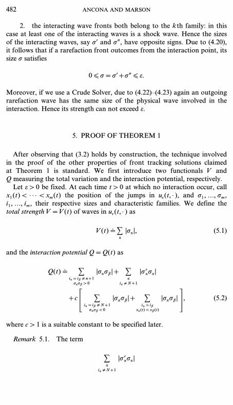
After observing that (3.2) holds by construction, the technique involvedin the proof of the other properties of front tracking solutions claimedat Theorem 1 is standard. We first introduce two functionals V andQ measuring the total variation and the interaction potential, respectively.

Let e > 0 be fixed. At each time t > 0 at which no interaction occur, callx1(t) < · · · < xm(t) the position of the jumps in ue(t, · ), and s1, ..., sm,i1, ..., im, their respective sizes and characteristic families. We define thetotal strength V=V(t) of waves in un(t, · ) as

V(t) qCa

|sa |, (5.1)

and the interaction potential Q=Q(t) as

Q(t) q Cia=ib ] n+1sasb > 0

|sasb |+ Ca

ia ] N+1

|s rasa |

+c r Cia=ib ] N+1sasb < 0

|sasb |+ Cia > ib

xa(t) < xb(t)

|sasb |s , (5.2)

where c > 1 is a suitable constant to be specified later.

Remark 5.1. The term

Ca

ia ] N+1

|s rasa |


in the above definition of the interaction potential takes into account of thepossible splitting, after an interaction, into two or more wavefronts of anincoming wave s belonging to a NGNL characteristic family, with

s rs s ] 0 or |s r| > e.

Indeed, in such a case the sizes of the new outgoing wavefronts cannot becontrolled by the size of the other interacting front, by means of (2.28) or(2.32) at Lemma 2.1.

5.1. Bound on the Total Variation

First we need a technical Lemma, whose proof is standard and relies onLemma 2.1.

Lemma 5.1. For any compact set K … W there exist constants C2, m2 > 0such that the following holds. Let ue=ue(t, x) be a piecewise constantapproximate solution of (1.1), constructed as above and defined on the strip[0, T[×R. Assume that Tot.Var.(ue(0, · )) < m2, limx Q −. u(0, x) ¥ K. Then

Tot.Var.(ue(t, · )) [ C2 Tot.Var.(ue(0, · )), -t > 0. (5.3)

Moreover, if at time y > 0 two wavefronts of sizes sŒ, sœ interact, then

DQ(y) [ −12 I(sŒ, sœ), (5.4)

DV(y)+2C1DQ(y) [ 0, (5.5)

with I(sŒ, sœ) defined at (2.26).

Proof. Let y be as in the assumptions and call iŒ, iœ the characteristicfamily of sŒ, sœ respectively. Assume that sŒ connect uL to uM, and sœuM touR Hence, from (2.27), (2.30), (4.24) we derive

DV(y)=V(y+)−V(y −) [ C1I(sŒ, sœ). (5.6)

Concerning Q, we will prove (5.4) only for I(sŒ, sœ) > r, and assumingthat both the iŒth and the iœth characteristic families are NGNL, the othercases being similar.

After time y the two fronts sŒ, sœ are no longer approaching. On theother hand new wavefronts, which appear after the interaction and belongto characteristic families different to both iŒ, iœ, may approach all the otherwaves. Call s ra, j the outgoing rarefaction fronts of the ath family,j=1, ..., ma, and s sa the outgoing shock front, whenever they exist. Here weconsider two cases


Case 1. iŒ ] iœ or iŒ=iœ=i and sŒsœ < 0. Assume iŒ ] iœ, the other casebeing similar. By definition

I(sŒ, sœ)=|sŒsœ|. (5.7)

Due to (2.28) we have

: |s −r|− Cmi Œ

j=1|s riŒ, j | : [ C1 min{|sŒ|, |sœ|},

| |s −s|− |s siŒ | | [ C1 min{|sŒ|, |sœ|},

whenever a composed wave of the iŒ th family outgoes. Entirely similarestimates hold for the iœth characteristic family. We obtain

DQ(y)−c |sŒsœ|− |s −rsŒ|− |s'rsœ|+12 Ca=iŒ, iœ

Cma

j, k=1|s ra, js

ra, k |

+ Ca=iŒ, iœ

1 |s sa | Cma

j=1|s ra, j |2+cC1 |sŒsœ| V(y −)

[ −(c−8C1 −4C21 −cC1V(y −)) |sŒsœ|.

By choosing

V(y −) <1

2C1, c > 1+16C1+8C2

1, (5.8)

we get (5.4).

Case 2. iŒ=iœ=i and sŒsœ > 0. For sake of simplicity, assume that(2.6) holds for k=i and that Dri li(uL) \ 0, the other cases being entirelysimilar. If

s −rs −s=s'rs's=0,

using Remark 4.2, we get (5.7). Hence, with arguments similar to the onesused above and choosing

V(y −) <1

2cC1, (5.9)

we get (5.4).Otherwise, due to Remark 4.1 we have

s −rs −s ] 0, sŒ > 0 sœ=s's > 0.


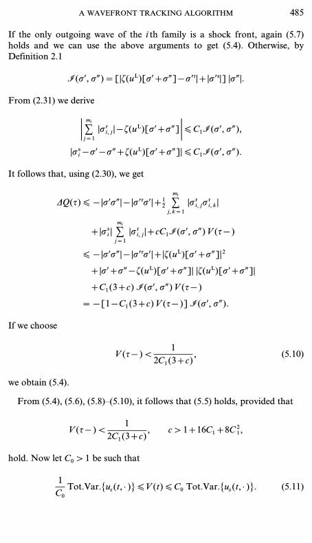
If the only outgoing wave of the ith family is a shock front, again (5.7)holds and we can use the above arguments to get (5.4). Otherwise, byDefinition 2.1

I(sŒ, sœ)=[|z(uL)[sŒ+sœ]− s −r|+|s −s|] |sœ|.

From (2.31) we derive

: Cmi

j=1|s ri, j | − z(uL)[sŒ+sœ] : [ C1I(sŒ, sœ),

|s si − sŒ− sœ+z(uL)[sŒ+sœ]| [ C1I(sŒ, sœ).

It follows that, using (2.30), we get

DQ(y) [ −|sŒsœ|− |s −rsŒ|+12 C

mi

j, k=1|s ri, js

ri, k |

+|s si | Cmi

j=1|s ri, j |+cC1I(sŒ, sœ) V(y −)

[ −|sŒsœ|− |s −rsŒ|+|z(uL)[sŒ+sœ]|2

+|sŒ+sœ− z(uL)[sŒ+sœ]| |z(uL)[sŒ+sœ]|

+C1(3+c) I(sŒ, sœ) V(y −)

=−[1−C1(3+c) V(y −)] I(sŒ, sœ).

If we choose

V(y −) <1

2C1(3+c), (5.10)

we obtain (5.4).

From (5.4), (5.6), (5.8)–(5.10), it follows that (5.5) holds, provided that

V(y −) <1

2C1(3+c), c > 1+16C1+8C2

1,

hold. Now let C0 > 1 be such that

1C0

Tot.Var.{ue(t, · )} [ V(t) [ C0 Tot.Var.{ue(t, · )}. (5.11)


Let

Tot.Var.{ue(0, · )} <1

3C0C1(1+2cC1)(3+c)q m2, (5.12)

and call y the first interaction time. We have

V(y −) [ C0 Tot.Var.{ue(0, · )} [1

3C1(1+2cC1)(3+c)<

12C1(3+c)

,

and hence, due to (5.5) and observing that Q(t) [ cV2(t) [ cV(t),

V(y+) [ V(y+)+2C1Q(y+) [ V(y −)+2C1Q(y −)

[1

3C1(3+c)<

12C1(3+c)

, (5.13)

holds. By an induction argument, (5.13), and hence (5.5), holds for anyy > 0. To complete the proof of the Lemma, we need to prove (5.3). Thisfollows easily from (5.5) and (5.11)–(5.12). Indeed

Tot.Var.{ue(t, · )} [ C0[V(t)+2C1Q(t)]

[ C0[V(0)+2C1Q(0)]

[ C0(1+2cC1) V(0)

[ C20(1+2cC1) Tot.Var.{ue(0, · )},

which is (5.3) with C2=C20(1+2cC1). L

From Lemma 5.1, (3.3) follows easily, provided that in (3.1) we choosed0=m2.

5.2. Bound on the Number of Wavefronts

Observe that new wavefronts can origin only at interaction points.Moreover, it suffices to prove that the total number of physical fronts isfinite. Indeed, a new nonphysical wavefront can origin only at the interac-tion between two physical fronts. Now, observe that, due to (5.4), the totalnumber of interactions involving two wavefronts sŒ, sœ such thatI(sŒ, sœ) > r, is finite, and by construction, when an interaction involves anonphysical wavefront, no new physical front outgoes. Hence we can takeinto account only of interactions involving two physical wavefronts sŒ, sœ

with I(sŒ, sœ) [ r. Moreover, due to definitions (4.17)–(4.20), whenever inthe outgoing wave fronts the strength of the rarefaction components do notexceed 3e, then the total number of physical wavefronts do not increase. It


follows that we can take into account only of interactions between twophysical fronts sŒ, sœ such that I(sŒ, sœ) [ r and at least one of thestrengths of the rarefaction components of the outgoing wavefronts isgreater than 3e. We claim that the total number of this kind of interactionsis finite. This follows from the next lemma.

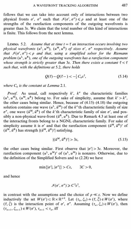
Lemma 5.2. Assume that at time t=y an interaction occurs involving twophysical wavefronts (uL, uM), (uM, uR) of sizes sŒ, sœ respectively. Assumethat I(sŒ, sœ) < r and that, using a simplified solver for the Riemannproblem (uL, uR), one of the outgoing wavefronts has a rarefaction componentwhose strength is strictly greater than 3e. Then there exists a constant y < y

such that, with the definitions at 5.2, there holds

Q(y)−Q(y −) < −12 C0e2, (5.14)

where C0 is the constant at Lemma 2.1.

Proof. As usual, call respectively kŒ, kœ the characteristic families(uL, uM), (uM, uR) belong to. For sake of simplicity, assume that kŒ > kœ,the other cases being similar. Hence, because of (4.15)–(4.18) the outgoingsolution contains one wave (uL, uM) of the kœth characteristic family of sizesœ, one wave (uM, uR) of the kŒ th characteristic family of size sŒ, and pos-sibly a non-physical wave-front (uR, uR). Due to Remark 4.3 at least one ofthe interacting fronts belong to a NGNL characteristic family. For sake ofsimplicity assume it is sŒ and that the rarefaction component (uM, uR) r of(uM, uR) has strength |(uM, uR) r| satisfying.

|(uM, uR) r| > 3e, (5.15)

the other cases being similar. First observe that |sŒ| > 3e. Moreover, therarefaction component (uL, uM) r of (uL, uM) is nonzero. Otherwise, due tothe definition of the Simplified Solvers and to (2.28) we have

min{|sŒ|, |sœ|} > Ce, ,C > 0,

and hence

I(sŒ, sœ) \ C2e2,

in contrast with the assumptions and the choice of r ° e. Now we defineinductively the set W(sŒ) … R×R\ 0. Let (y0, t0) q (y, t) ¥ W(sŒ), where(y, t) is the interaction point of sŒ, sœ. Assuming (yn, tn) ¥ W(sŒ), then(yn+1, tn+1) ¥ W(sŒ), yn+1 < yn, iff


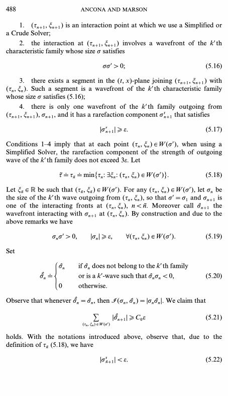
1. (yn+1, tn+1) is an interaction point at which we use a Simplified ora Crude Solver;

2. the interaction at (yn+1, tn+1) involves a wavefront of the kŒthcharacteristic family whose size s satisfies

ssŒ > 0; (5.16)

3. there exists a segment in the (t, x)-plane joining (yn+1, tn+1) with(yn, tn). Such a segment is a wavefront of the kŒ th characteristic familywhose size s satisfies (5.16);

4. there is only one wavefront of the kŒ th family outgoing from(yn+1, tn+1), sn+1, and it has a rarefaction component s rn+1 that satisfies

|s rn+1 | \ e. (5.17)

Conditions 1–4 imply that at each point (yn, tn) ¥ W(sŒ), when using aSimplified Solver, the rarefaction component of the strength of outgoingwave of the kŒth family does not exceed 3e. Let

y q yn q min{yn: ,tn: (yn, tn) ¥ W(sŒ)}. (5.18)

Let tn ¥ R be such that (yn, tn) ¥ W(sŒ). For any (yn, tn) ¥ W(sŒ), let sn bethe size of the kŒth wave outgoing from (yn, tn), so that sŒ=s1 and sn+1 isone of the interacting fronts at (yn, tn), n < n. Moreover call sn+1 thewavefront interacting with sn+1 at (yn, tn). By construction and due to theabove remarks we have

snsŒ > 0, |sn | \ e, -(yn, tn) ¥ W(sŒ). (5.19)

Set

sn q ˛sn if sn does not belong to the kŒth family

or is a kŒ-wave such that snsn < 0,0 otherwise.

(5.20)

Observe that whenever sn=sn, then I(sn, sn)=|snsn |. We claim that

C(yn, tn) ¥ W(sŒ)

|sn+1 | \ C0e (5.21)

holds. With the notations introduced above, observe that, due to thedefinition of yn (5.18), we have

|s rn+1 | < e. (5.22)


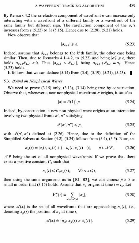
By Remark 4.2 the rarefaction component of wavefront s can increase onlyinteracting with a wavefront of a different family or a wavefront of thesame family but different sign. The rarefaction component of the sn’sincreases from e (5.22) to 3e (5.15). Hence due to (2.28), (5.21) holds.

Now observe that

|sn+1 | \ e. (5.23)

Indeed, assume that sn+1 belongs to the kŒ th family, the other case beingsimilar. Then, due to Remarks 4.1–4.2, to (5.22) and being |s r

n | \ e, thereholds sn+1sn+1 < 0. Thus |sn+1 | > |sn+1 |, being sn+1+sn+1=sn. Hence(5.23) holds.

It follows that we can deduce (5.14) from (5.4), (5.19), (5.21), (5.23). L

5.3. Bound on Nonphysical Waves

We need to prove (3.15) only, (3.13), (3.14) being true by construction.Observe that, whenever a new nonphysical wavefront s origins, it satisfies

|s|=O(1) · r. (5.24)

Indeed, by construction, a new non-physical wave origins at an interactioninvolving two physical fronts sŒ, sœ satisfying

I(sŒ, sœ) [ r, (5.25)

with I(sŒ, sœ) defined at (2.26). Hence, due to the definition of theSimplified Solvers at Section (4.2), (5.24) follows from (5.4), (5.5). Now, set

sa(t)=|ue(t, xa(t)+)−ue(t, xa(t)−)|, a ¥NP, (5.26)

NP being the set of all nonphysical wavefronts. If we prove that thereexists a positive constant C3 such that

sa(t) [ C3sa(s), -0 < s [ t, (5.27)

then using the same arguments as in [BJ, B2], we can choose r > 0 sosmall in order that (3.15) holds. Assume that sa origins at time t=ta. Let

Vga (t) q C

sa ¥A(a)|sa |, (5.28)

where A(a) is the set of all wavefronts that are approaching sa(t), i.e.,denoting xb(t) the position of sb at time t,

A(a) q {sb: xb(t) > xa(t)}. (5.29)


Now consider an interaction time y > ta. Two cases can occur:

1. The interaction does not involve sa. Then, due to (5.5), we have

Dsa(y)=0, DVga (y)+2C1DQ(y) [ 0. (5.30)

2. The interaction does involve sa. Call sb the other interactingwavefront. Then, due to the definition of Vg

a (5.28)–(5.29), to (5.4) and tothe interaction estimates at Lemma 2.1, we deduce that there exists apositive constant c2 such that

DVga (y)=−|sb |, DQ(y) < 0, |Dsa(y)| [ c2sa(y −) |sb |. (5.31)

In any case, we can choose a positive constant c3 in order to make the map

t W sa(t) exp{c3[Vga (t)+2C1Q(t)]},

decreasing. Hence, if t > s, we have

sa(t) [ sa(s) exp{c3[Vga (s)−Vg

a (t)+2C1(Q(s)−Q(t))]},

from which (5.27) follows, due to (3.3).

5.4. Estimates on Shock and Rarefaction Fronts

First we need a preliminary Lemma.

Lemma 5.3. There exists r > 0 such that, in connection with the con-struction of an approximate solution ue=ue(t, x) at Section 4.3, the followingholds. Let l be chosen as in (3.14). Let x=xl(t) be any time-like polygonalline in the (t, x)-plane with slope strictly less than l, i.e.,

|xl(t)| < l. (5.32)

Call x1(t), ..., xn(t) the nonphysical wavefronts in the approximate solutionue. Let (ta, xa), ta \ 0, a=1, ..., n be the intersecting point in the (t, x) planeof x=xa(t) with x=xl(t), whenever it exists, i.e.,

xa(ta)=xl(ta)=xa, a=1, ..., n. (5.33)

Then we have

Cn

a=1|ue(ta, xa+)−ue(ta, xa−)|=O(1) · e. (5.34)


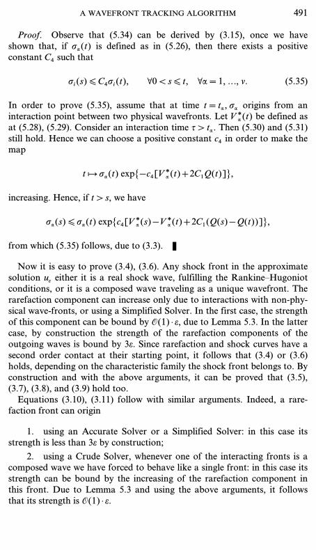
Proof. Observe that (5.34) can be derived by (3.15), once we haveshown that, if sa(t) is defined as in (5.26), then there exists a positiveconstant C4 such that

si(s) [ C4si(t), -0 < s [ t, -a=1, ..., n. (5.35)

In order to prove (5.35), assume that at time t=ta, sa origins from aninteraction point between two physical wavefronts. Let Vg

a (t) be defined asat (5.28), (5.29). Consider an interaction time y > ta. Then (5.30) and (5.31)still hold. Hence we can choose a positive constant c4 in order to make themap

t W sa(t) exp{−c4[Vga (t)+2C1Q(t)]},

increasing. Hence, if t > s, we have

sa(s) [ sa(t) exp{c4[Vga (s)−Vg

a (t)+2C1(Q(s)−Q(t))]},

from which (5.35) follows, due to (3.3). L

Now it is easy to prove (3.4), (3.6). Any shock front in the approximatesolution ue either it is a real shock wave, fulfilling the Rankine–Hugoniotconditions, or it is a composed wave traveling as a unique wavefront. Therarefaction component can increase only due to interactions with non-phy-sical wave-fronts, or using a Simplified Solver. In the first case, the strengthof this component can be bound by O(1) · e, due to Lemma 5.3. In the lattercase, by construction the strength of the rarefaction components of theoutgoing waves is bound by 3e. Since rarefaction and shock curves have asecond order contact at their starting point, it follows that (3.4) or (3.6)holds, depending on the characteristic family the shock front belongs to. Byconstruction and with the above arguments, it can be proved that (3.5),(3.7), (3.8), and (3.9) hold too.

Equations (3.10), (3.11) follow with similar arguments. Indeed, a rare-faction front can origin

1. using an Accurate Solver or a Simplified Solver: in this case itsstrength is less than 3e by construction;

2. using a Crude Solver, whenever one of the interacting fronts is acomposed wave we have forced to behave like a single front: in this case itsstrength can be bound by the increasing of the rarefaction component inthis front. Due to Lemma 5.3 and using the above arguments, it followsthat its strength is O(1) · e.


Hence at the origin the strength of a rarefaction front is O(1) · e. Following[B2] and with arguments similar to the ones used for the non-physicalfronts, it can be proved that an estimate similar to (5.27) holds for a rare-faction front, proving (3.10)1 and (3.11)1. Moreover, (3.10)2, (3.10)2, and(3.12) hold by construction.

This ends the proof of Theorem 1.

REFERENCES

[AM1] F. Ancona and A. Marson, A note on the Riemann problem for general n×nsystems of conservation laws, J. Math. Anal. Appl., in press.

[AM2] F. Ancona and A. Marson, Basic estimates for a front tracking algorithm forgeneral 2×2 conservation laws, Math. Models Methods Appl. Sci., in press.

[AM3] F. Ancona and A. Marson, Well-posedness for general 2×2 systems of conservationlaws, Mem. Amer. Math. Soc., in press.

[AM4] F. Ancona and A. Marson, Well-posedness for non genuinely nonlinear conserva-tion laws, in ‘‘Proc. 8th Intern. Conf. on Hyperb. Probl.—Theory Numeric andAppl., Magdeburg,’’ in press.

[AM5] F. Ancona and A. Marson, L1-Stability of weak solutions for N×N non genuinelynonlinear conservation laws, preprint, 2000.

[BJ] P. Baiti and H. K. Jenssen, On the front-tracking algorithm, J. Math. Anal. Appl.217 (1998), 395–404.

[B1] A. Bressan, Global solutions to systems of conservation laws by wave-fronttracking, J. Math. Anal. Appl. 170 (1992), 414–432.

[B2] A. Bressan, ‘‘Hyperbolic Systems of Conservation Laws—The One-DimensionalCauchy Problem,’’ Oxford Univ. Press, Oxford, in press.

[B3] A. Bressan, The unique limit of the Glimm scheme, Arch. Rational Mech. Anal. 130(1995), 205–230.

[B-G] A. Bressan and P. Goatin, Oleinik type estimates and uniqueness for n×n conser-vation laws, J. Differential Equations 156 (1999), 26–49.

[B-L] A. Bressan and M. Lewicka, A uniqueness condition for hyperbolic systems ofconservation laws, Discrete Contin. Dynam. Systems 6 (2000), 673–682.

[BLY] A. Bressan, T. P. Liu, and T. Yang, L1 stability estimates for n×n conservationlaws, Arch. Rational Mech. Anal. 149 (1999), 1–22.

[BM] A. Bressan and A. Marson, Error bounds for a deterministic version of the Glimmscheme, Arch. Rational Mech. Anal. 142 (1998), 155–176.

[Da] C. Dafermos, Polygonal approximations of solutions of the initial value problem fora conservation law, J. Math. Anal. Appl. 38 (1972), 33–41.

[Dp1] R. DiPerna, Global existence of solutions to nonlinear hyperbolic systems ofconservation laws, J. Differential Equations 20 (1976), 187–212.

[Dp2] R. DiPerna, Uniqueness of solutions to hyperbolic conservation laws, Indiana Univ.Math. J. 28 (1979), 137–188.

[Gl] J. Glimm, Solutions in the large for nonlinear hyperbolic systems of equations,Comm. Pure Appl. Math. 18 (1965), 697–715.

[La] P. D. Lax, Hyperbolic systems of conservation laws II, Comm. Pure Appl. Math. 10(1957), 537–566.

[Li1] T. P. Liu, The Riemann problem for general 2×2 conservation laws, Trans. Amer.Math. Soc. 199 (1974), 89–112.


[Li2] T. P. Liu, The Riemann problem for general systems of conservation laws,J. Differential Equations 18 (1975), 218–234.

[Li3] T. P. Liu, Admissible solutions of hyperbolic conservation laws, Mem. Amer. Math.Soc. 30 (1981), no. 240.

[L-Y] T. P. Liu and T. Yang, Weak solutions of general systems of hyperbolic conser-vation laws, submitted.

[R] N. H. Risebro, A front-tracking alternative to the random choice method, Proc.Amer. Math. Soc. 117 (1993), 1125–1139.

[RMS1] T. Ruggeri, A. Muracchini, and L. Seccia, Continuum approach to phonon gas andshape changes of second sound via shock waves theory, Nuovo Cimento D 16 (1994),15–44.

[RMS2] T. Ruggeri, A. Muracchini, and L. Seccia, Second sound and characteristictemperature in solids, Phys. Rev. B 54 (1996), 332–339.

[Sm] J. Smoller, ‘‘Shock Waves and Reaction-Diffusion Equations,’’ second ed., Springer-Verlag, Berlin, 1994.


A Wavefront Tracking Algorithm for N×N Nongenuinely Nonlinear Conservation Laws

Documents

Transcript of A Wavefront Tracking Algorithm for N×N Nongenuinely Nonlinear Conservation Laws