The Geometry of Wul� Crystal Shapes and ItsRelations with Riemann Problems�Danping Peng, Stanley Osher, Barry Merriman, Hong-Kai ZhaoDepartment of MathematicsUniversity of CaliforniaLos Angeles, CA 90095-1555December 8, 1998AbstractIn this paper we begin to explore the mathematical connection between equilibriumshapes of crystalline materials (Wul� shapes) and shock wave structures in compressiblegas dynamics (Riemann problems). These are radically di�erent physical phenomena,but the similar nature of their discontinuous solutions suggests a connection.We show there is a precise sense in which any two dimensional crystalline formcan be described in terms of rarefactions and contact discontinuities for an associatedscalar hyperbolic conservation law. As a byproduct of this connection, we obtain a newanalytical formula for crystal shapes in two dimension. We explore a possible extensionto high dimensions.We also formulate the problem in the level set framework and present a simplealgorithm using the level set method to plot the approximate equilibrium crystal shapecorresponding to a given surface energy function in two and three dimensions.Our greater motivation for establishing this connection is to encourage a transferof theoretical and numerical techniques between the rich but disparate disciplines ofcrystal growth and gas dynamics. The work reported here represents a �rst steptowards this goal.Contents1 Introduction 22 The Wul� Problem and the Legendre Transformation 52.1 The Formulation of Wul� Problem . . . . . . . . . . . . . . . . . . . . . . . 52.2 Wul�'s Geometric Construction of the Solution . . . . . . . . . . . . . . . . 62.3 The Wul� Shape and the Legendre Transformation . . . . . . . . . . . . . . 72.4 Growing a Wul� Crystal . . . . . . . . . . . . . . . . . . . . . . . . . . . . . 142.5 Typical Forms for Surface Tension . . . . . . . . . . . . . . . . . . . . . . . . 14�Research supported by DARPA/NSF VIP grant:NSF grant DMS9615854 and NSF grant DMS9706827.1

3 The Wul� Crystal Shape in 2D 163.1 The Legendre Transformation in 2D . . . . . . . . . . . . . . . . . . . . . . . 163.2 The Euler-Lagrange Equation . . . . . . . . . . . . . . . . . . . . . . . . . . 193.3 Multivalued Solutions . . . . . . . . . . . . . . . . . . . . . . . . . . . . . . . 203.4 Frank's Convexi�cation of Surface Tension . . . . . . . . . . . . . . . . . . . 213.5 Two Formulae for the Normal Direction . . . . . . . . . . . . . . . . . . . . 234 The Riemann Problem 254.1 The Riemann Problem Formulation . . . . . . . . . . . . . . . . . . . . . . . 254.2 Multiple-Valued Solutions . . . . . . . . . . . . . . . . . . . . . . . . . . . . 264.3 Geometric Construction of the Solution . . . . . . . . . . . . . . . . . . . . . 275 The 2D Wul� Crystal as the Solution of a Riemann Problem 285.1 From the Euler-Lagrange Equation to a Scalar Conservation Law . . . . . . 295.1.1 The Basic Connection . . . . . . . . . . . . . . . . . . . . . . . . . . 295.1.2 Di�erences Between Wul� and Riemann Jump Conditions . . . . . . 305.1.3 Reparameterization of Euler-Lagrange Equation . . . . . . . . . . . . 315.2 Self-Similar Growth of Wul� Shape and Riemann Problem . . . . . . . . . . 325.3 Main Theorem and Its Consequences . . . . . . . . . . . . . . . . . . . . . . 335.4 A Convex Example . . . . . . . . . . . . . . . . . . . . . . . . . . . . . . . . 345.5 A Nonconvex Example . . . . . . . . . . . . . . . . . . . . . . . . . . . . . . 386 Some Comments on The Wul� Problem in Higher Dimensions 407 The Level Set Formulation for the Wul� Problem 407.1 The Level Set Representation of Surface Energy . . . . . . . . . . . . . . . . 407.2 The Euler-Lagrange Equation for the Wul� Problem . . . . . . . . . . . . . 417.3 The Hamilton-Jacobi Equation for a Growing Wul� Crystal . . . . . . . . . 428 Numerical Examples 429 Appendix 51I Proof of Lemma 2 . . . . . . . . . . . . . . . . . . . . . . . . . . . . . . . . . 51II The Evolution Equation for the Normal Angle in 2D . . . . . . . . . . . . . 54III The Euler-Lagrange Equation of Surface Energy . . . . . . . . . . . . . . . . 571 IntroductionIn this paper we develop a mathematical connection between two quite di�erent physicalphenomena: the shapes of crystalline materials, and dynamics of shock waves in a gas.Both of these phenomena have long research histories: The problem of determining theequilibrium shape of a perfect crystal was posed and �rst solved by Wul� in 1901 [26]. Innature this ideal \Wul� shape" (see �gure 1) is observed in crystals that are small enoughto relax to their lowest energy state without becoming stuck in local minima.2

(a) −1 −0.5 0 0.5 1−1

−0.8

−0.6

−0.4

−0.2

0

0.2

0.4

0.6

0.8

1

(b)Figure 1: (a) A 2D Wul� crystal. (b) A 3D Wul� crystal.The problem of determining the dynamics of a gas initialized with an arbitrary initialjump in state was posed and partially solved by Riemann in 1860 [19]. Solutions to this\Riemann problem" can be observed experimentally in shock tubes, where a membraneseparating gases in di�erent uniform states is rapidly removed. The Riemann problem hassince been generalized to mean the solution of any system of hyperbolic conservation lawssubject to initial data prepared with a single jump in state separating two regions withdi�erent constant states.The intuitive link between Wul� crystals and Riemann problems is the similar natureof the discontinuous solutions. Crystalline shapes are characterized by perfectly at faces|facets|separated by sharp edges, whereas shocked gases are characterized by regions ofconstant pressure separated by steep jumps. Refer to �gure 2. It is tempting to imaginethat the sharp edges in a crystal shape can be though of as shock waves in some sense.To explore this shock wave-crystal edge analogy more precisely, we represent the crystalsurface by its unit normal vector. The normal has regions of constant direction separatedby jumps in direction, which suggests it may be governed by the same sort of equations|hyperbolic conservation laws|that govern shocks in nonlinear gas dynamics. The analogycontinues to hold if we consider the most general behaviors of Wul� crystals and Riemannproblems: Wul� shapes are constructed entirely from facets, rounded faces and sharp edges,for which the normal direction has regions of constancy, smooth variation, and isolatedjumps. Correspondingly, the solution to a Riemann problem for any hyperbolic conservationlaw is constructed entirely from constant states, rarefactions (smooth variation), and shocksor contacts (isolated jumps).We will show that the precise connection is this: the normal vector to the Wul� shapeof a crystal in two dimensions is the time self-similar solution of an associated Riemannproblem for a hyperbolic conservation law. In this representation, it does indeed turn out3

ν = π/2

ν = 0ν = π

n

n

n

n

ν = 3π/2

θ

ν = 2π

3π/4π/4 5π/4 7π/4 2π

π/2

π

3π/2

2π

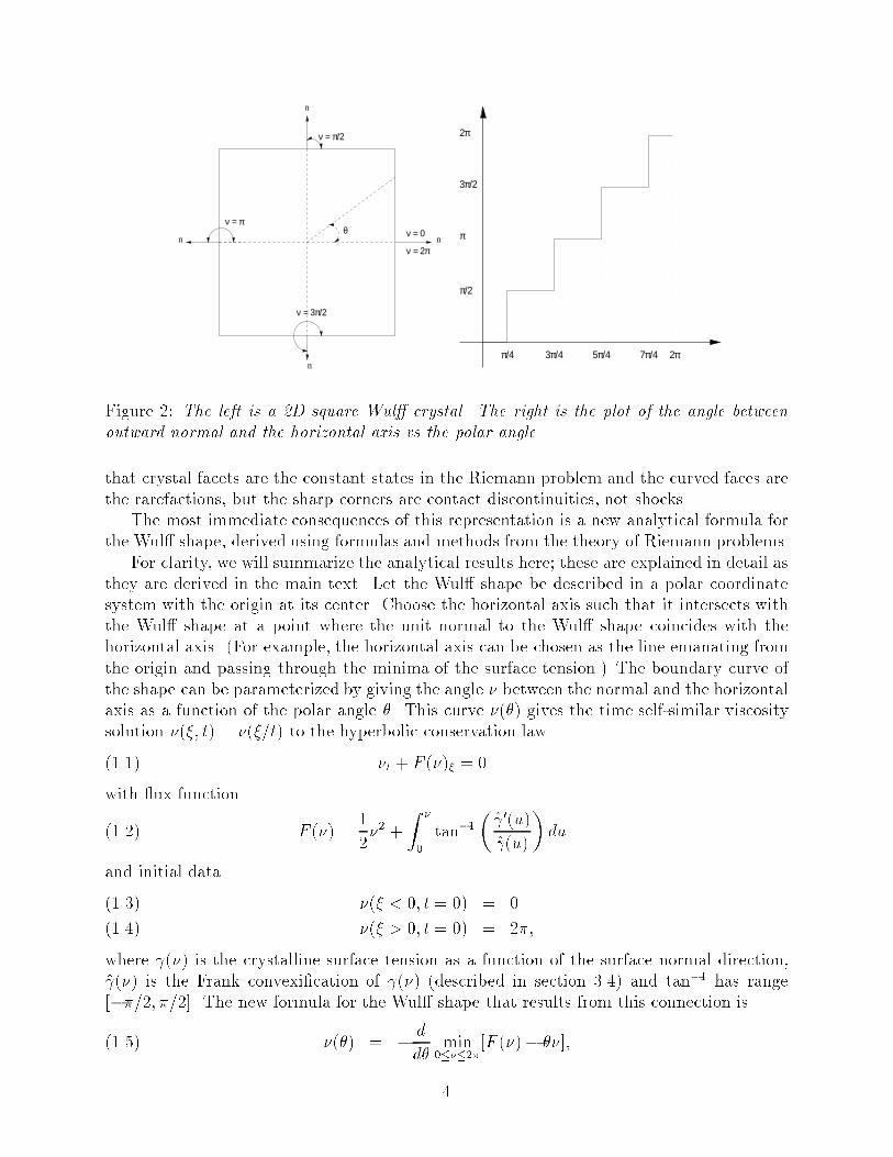
Figure 2: The left is a 2D square Wul� crystal. The right is the plot of the angle betweenoutward normal and the horizontal axis vs the polar angle.that crystal facets are the constant states in the Riemann problem and the curved faces arethe rarefactions, but the sharp corners are contact discontinuities, not shocks.The most immediate consequences of this representation is a new analytical formula forthe Wul� shape, derived using formulas and methods from the theory of Riemann problems.For clarity, we will summarize the analytical results here; these are explained in detail asthey are derived in the main text. Let the Wul� shape be described in a polar coordinatesystem with the origin at its center. Choose the horizontal axis such that it intersects withthe Wul� shape at a point where the unit normal to the Wul� shape coincides with thehorizontal axis. (For example, the horizontal axis can be chosen as the line emanating fromthe origin and passing through the minima of the surface tension.) The boundary curve ofthe shape can be parameterized by giving the angle � between the normal and the horizontalaxis as a function of the polar angle �. This curve �(�) gives the time self-similar viscositysolution �(�; t) = �(�=t) to the hyperbolic conservation law�t + F (�)� = 0(1.1)with ux function F (�) = 12�2 + Z �0 tan�1� 0(u) (u)� du(1.2)and initial data �(� < 0; t = 0) = 0(1.3) �(� > 0; t = 0) = 2�;(1.4)where (�) is the crystalline surface tension as a function of the surface normal direction, (�) is the Frank convexi�cation of (�) (described in section 3.4) and tan�1 has range[��=2; �=2]. The new formula for the Wul� shape that results from this connection is�(�) = � dd� min0���2�[F (�)� ��];(1.5) 4

where F is the ux function from the conservation law.The primary goal of this paper is to expose the connection between faceted crystal shapesand shock waves and related phenomena from gas dynamics. Because readers familiar withthe theory of Wul� shapes come from a materials science background, they are unlikely toknow the theory of Riemann problems from the �eld of gas dynamics, and vice versa. To �llin these likely gaps, we will present the elementary background for both problems prior toderiving our new results. In addition to making the present paper more readable, we hopethis inclusive approach will foster future interaction between these two disparate researchcommunities.The paper is organized as follows: we start with the essential background on the Wul�problem and the Riemann problem, emphasizing their similarities. Then we show how torepresent the Wul� shape as the solution to a Riemann problem, via two seemingly quitedi�erent approaches: the �rst approach starts from the Euler-Lagrange equation of thesurface energy and connects it with the Riemann problem of a scalar conservation law undera suitable choice of variables. The other approach uses the self-similar growth property of theWul� shape and shows that it solves a Riemann problem for the same conservation law. Inthe process, we develop the new formula (1.5). We present two simple illustrative examplesand comment on further possible extensions of these ideas. We then formulate the Wul�problem in the level set setting and use it to derive some theoretical results about Wul�shape. This method is also a convenient and versatile tool for plotting the Wul� shape ofa given surface tension function in both two and three dimensions. We present numerousexamples demonstrating this and verify some recently obtained theoretical results in [17]concerning the Wul� shape in the numerical section. The appendix contains proofs of someresults in the main text that require certain degrees of technicality.2 The Wul� Problem and the Legendre Transforma-tionThis section will brie y review and develop some general results about the Wul� crystalshape that are valid in any dimension. The next section will concentrate on the Wul�crystal shape in 2D.2.1 The Formulation of Wul� ProblemThe Wul� problem is to determine the equilibrium shape of a perfect crystal of one materialin contact with a single surrounding medium. The equilibrium shape is determined byminimizing the total system energy, which is composed of contributions from the bulk andsurface of the crystal. If we consider a �xed volume of material, the bulk energy is also �xed,and the problem becomes that of �nding a shape of given volume with minimal surfaceenergy.If the surface energy density|that is, the \surface tension"|is constant, the solutionis the shape of minimal surface area, which is a circle in 2D and a sphere in 3D. However,in many solid materials the surface tension depends on how the surface is directed relativeto the bulk crystalline lattice, due to the detailed structure of the bonding between atoms.5

Assuming some standard orientation of the bulk lattice, the surface tension, , will be ade�nite function of the normal vector to the surface, n, say = (n). In that case, if thematerial is bounded by a surface �, the total surface energy isE = Z� (n)dA;(2.1)which must be minimized subject to the constraint of constant volume enclosed by �.This problem makes sense both in two and three dimensions, and essentially 2D crystalsdo arise experimentally in the growth of thin �lms. The formula we derive in this sectionapplies equally well in both dimensions. In the next section, we will concentrate our attentionon the 2D problem, where we can make the precise connection to a Riemann problem. Inthis case, (n) is the energy per unit length on the boundary, and we we seek to determinethe bounding curve, �, of minimal surface energy that encloses a given area.2.2 Wul�'s Geometric Construction of the SolutionWul� presented the solution to this minimization problem as an ingenious geometric con-struction, based on the geometry of the surface tension. Let : Sd�1 ! R+ be the surfacetension which is a continuous function, where d = 2 or 3. Wul�'s construction is as follows(refer to �gure 3):p

p

Figure 3: Wul�'s geometric construction.� Step 1. Construct a \polar plot" of (�). In 2D, this is simply the curve de�ned inr-� polar coordinates by r = (�), 0 � � � 2�. In 3D, this is a surface around theorigin in sphere coordinates r-�. 6

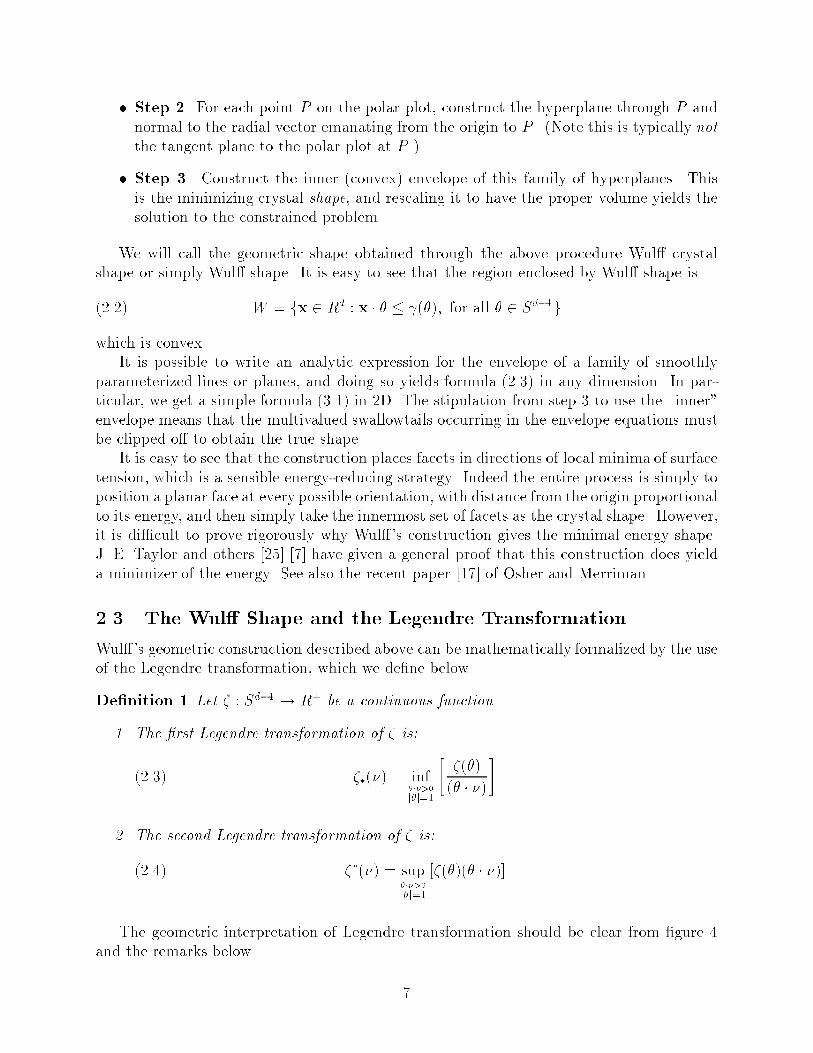
� Step 2. For each point P on the polar plot, construct the hyperplane through P andnormal to the radial vector emanating from the origin to P . (Note this is typically notthe tangent plane to the polar plot at P .)� Step 3. Construct the inner (convex) envelope of this family of hyperplanes. Thisis the minimizing crystal shape, and rescaling it to have the proper volume yields thesolution to the constrained problem.We will call the geometric shape obtained through the above procedure Wul� crystalshape or simply Wul� shape. It is easy to see that the region enclosed by Wul� shape isW = fx 2 Rd : x � � � (�); for all � 2 Sd�1g(2.2)which is convex.It is possible to write an analytic expression for the envelope of a family of smoothlyparameterized lines or planes, and doing so yields formula (2.3) in any dimension. In par-ticular, we get a simple formula (3.1) in 2D. The stipulation from step 3 to use the \inner"envelope means that the multivalued swallowtails occurring in the envelope equations mustbe clipped o� to obtain the true shape.It is easy to see that the construction places facets in directions of local minima of surfacetension, which is a sensible energy-reducing strategy. Indeed the entire process is simply toposition a planar face at every possible orientation, with distance from the origin proportionalto its energy, and then simply take the innermost set of facets as the crystal shape. However,it is di�cult to prove rigorously why Wul�'s construction gives the minimal energy shape.J. E. Taylor and others [25] [7] have given a general proof that this construction does yielda minimizer of the energy. See also the recent paper [17] of Osher and Merriman.2.3 The Wul� Shape and the Legendre TransformationWul�'s geometric construction described above can be mathematically formalized by the useof the Legendre transformation, which we de�ne below.De�nition 1 Let � : Sd�1 ! R+ be a continuous function.1. The �rst Legendre transformation of � is:��(�) = inf���>0j�j=1 � �(�)(� � �)�(2.3)2. The second Legendre transformation of � is:��(�) = sup���>0j�j=1 [�(�)(� � �)](2.4)The geometric interpretation of Legendre transformation should be clear from �gure 4and the remarks below. 7

νθζ(θ)θν ζ(θ)

Figure 4: Left: the �rst Legendre transformation. The solid line is the plot of �, and thedashed line is the plot of ��, the corresponding Wul� shape. Right: second Legendre trans-formation. The solid line is the plot of �, and the dashed line is the plot of ��, the supportfunction.Remark 1. The �rst Legendre transformation ��(�) gives the Wul� crystal shape. This iseasy to see from equation (2.2) in polar coordinates:W = f(r; �) : r(� � �) � �(�); for all � 2 Sd�1g= f(r; �) : r � inf���>0j�j=1 � �(�)(� � �)�g= f(r; �) : r � ��(�)gRemark 2. The second Legendre transformation ��(�) gives the support function of theregion enclosed by the polar plot of �. Recall that the support function p of a boundedregion which contains the origin is de�ned byp(�) = maxfx � � : x 2 g; for � 2 Sd�1(2.5)We will see shortly that the �rst and second Legendre transformation are dual to eachother in certain sense. The following relations are obvious by de�nition:Lemma 1 ��(�) � �(�) � ��(�)(2.6) 1�� = �1��� ; 1�� = �1���(2.7) 8

Since � is de�ned on a curved space Sd�1, sometimes it is convenient to study the exten-sion of � to the whole Rd. We extend � : Sd�1 ! R+ to Rd by de�ning��(x) = jxj�( xjxj); for x 2 Rd(2.8)Such an extension �� is homogeneous of degree 1. If �� is di�erentiable, we have the followingimportant relation due to Euler: nXj=1 xj @��@xj (x) = ��(x)(2.9)Note that each of the �rst partial derivatives of �� is homogeneous of degree 0, and the secondpartial derivatives are homogeneous of degree �1. We will abuse the notation and write ��as � when no ambiguity arise.De�nition 2 � is convex if the polar plot of 1� is convex. � is polar convex if the polar plotof � is convex.The following lemma gives the necessary and su�cient condition for � to be convex interm of its extension.Lemma 2 � is convex if and only if its homogeneous extension of degree 1 �� : Rd ! R+ isa convex function on Rd.See Appendix I for the proof.As we have seen, the Wul� shape W = f x : jxj � ��( xjxj) g is always convex. Byde�nition, �� is polar convex. From lemma 1, �� is convex. We put these facts inLemma 3 �� is always polar convex and �� is always convex.Now let us introduce �(�) = (��)�(�) , ��(�) = (��)�(�)(2.10)From the de�nitions and the lemma above, we know that � is always convex and ��polar-convex.De�nition 3 We call �(�) the Frank convexi�cation of �, and ��(�) the polar convexi�cationof �.We proceed to prove the following important relations:Lemma 4 �(�) � �(�) � ��(�)(2.11) �1��^ = 1�� ; �1��_ = 1�(2.12) 9

Proof: From the de�nition,�(�) = sup���>0[��(�)(� � �)] = sup��� [( inf���>0 �(�)(� � �)(� � �)]� sup���>0[ �(�)(� � �)(� � �)] = �(�)The other inequality can be proved similarly.The key ingredient in proving the two equalities is the repeated use of the duality relations(2.7): �1��^ = ��1����� = � 1���� = 1= 1� 1����= 1= 11�� !� = 1(��)� = 1��The other equality follows from the above and the duality relations (2.7).Both � and �� have simple geometric interpretations. From the de�nition, the steps usedto obtain �� can be described in words as following: draw the polar-plot � of �. Let be theregion enclosed by �. Through each point on �, draw the hyperplane(s) tangent to � whichlie outside . Note that such a plane may not exist, such as at points that curved inward, andmay not be unique, such as at the points that bulge outward. This corresponds to the stepsused in constructing the support function. Then �nd the inner envelope of all such tangentplanes. This corresponds to the construction of the Wul� shape of the support function.The inner envelope is the smallest convex set that contains , i.e. the convexi�cation of. We thus get a simple procedure to obtain �� : plot the graph of � in polar coordinates,convexify the plot and obtain a convex graph. This is the polar plot of ��. Using the dualityrelation (2.12), we can obtain � by �rst drawing the polar plot of 1� , then convexifying theregion enclosed to get �1��_ = 1� , then inverting it to get �. See the �gures in section 5.5.These arguments show thatLemma 5 If � is convex, then � = �. If � is polar-convex, then �� = �.We now show the following importantTheorem 1 1. The Wul� shape of � and � are the same. That is,���� = ��(2.13)2. The support function of � and �� are the same. That is,����� = ��(2.14) 10

Proof: We already know that � � �. Hence (�)� � ��. One the other hand,�(�) = max���>0j�j=1[��(�)(� � �)] � ��(�)(� � �); for all � 2 Sd�1Using this inequality and the de�nitions, we have:(�)�(�) = inf���>0j�j=1" �(�)(� � �)# � inf���>0j�j=1 ���(�)(� � �)(� � �) � = ��(�)From the above discussion, we see that given a convex body K � Rd, the surface tensionwhose Wul� shape is K is not uniquely de�ned. However, if we require that the surfacetension is convex, then it is uniquely determined by K. If the boundary of K is given byr : Sd�1 ! R+, then the convex surface tension function whose Wul� shape is K is given bythe second Legendre transformation = r�.Now let us further assume that � : Sd�1 ! R+ is a C1 function. We extend � to Rdto be a homogeneous function of degree 1. Then the �rst Legendre transformation can berewritten as ��(�) = infx��>0 ��(x)x � � � = infx��>0 � � xx � ��(2.15)Suppose the in�mum is reached at certain x = x(�) 2 Rd, and let p = xx�� . We have0 = @@xi� � xx � �� =Xj @�@pj @pj@xi= Xj @�@pj � �ijx � � � �ixj(x � �)2�= @�@pi 1x � � � Xj @�@pj pj! �ix � �= 1x � � � @�@pi � �(p)�i�using relation (2.9). Thus we have �(p)�i = @�@pi (p)Since p = xx�� = nn�� , where n = n(�) is the unit normal to the Wul� shape at R = ��(�)�,and ��(�) = �(n)n�� , we get ��(�)� = D�(n)(2.16) ��(�) = jD�(n)j(2.17) � = D�(n)jD�(n)j(2.18) 11

For a given �, the n determined by (2.18) may not be unique unless � is strictly convex.Equation (2.16) gives us a convenient way to get the Wul� shape for a given surfacetension function . We simply draw the surface (in 3D) or curve (in 2D) parameterized byn. The surface or curve will generally self-intersect, except when is convex. We may clipo� the intersecting part, and obtain the Wul� crystal shape. See next section for examplesin 2D.There are equally simple relations for the second Legendre transformation. From theduality relations (2.7), we have 1��(n) = jD1� (�)jn = D��1jD��1j(�)Note that here it is 1=� that is extended as a homogeneous function of degree 1, and hence� itself is extended as a homogeneous function of degree �1. From the above relations, weget ��(n)n = ��2D�jD�j2 (�)(2.19) ��(n) = �2jD�j(�)(2.20) n = � D�jD�j(�)(2.21)Let us look at two examples.Example 1. In 2D, the surface tension function is usually given in term of the angle � ofnormal n to a �xed horizontal axis, i.e. = (�). We extend as a homogeneous functionof degree 1 in the following way (x; y) =px2 + y2 (tan�1 yx)(2.22)and easily get �(�)n(�) = D (�) = (�)n(�) + 0(�)� (�)(2.23)where n(�) = (cos �; sin �)� (�) = (� sin �; cos �)When is convex, that is when + 00 � 0 , equation (2.23) is a parameterization of theWul� shape in term of � and the �rst Legendre transformation of is given by �(�) =p 2(�) + 02(�)(2.24) 12

where � is determined by � = � + tan�1� 0(�) (�)�(2.25)See section 3 for details.To �nd the second Legendre transformation, we extend to the whole space as a homo-geneous function of degree �1 by de�ning (x; y) = 1px2 + y2 (tan�1 yx)(2.26)From the general relations (2.19){(2.21), we obtain �(�)n(�) = 2(�) 2(�) + 02(�) [ (�)n(�)� 0(�)� (�)](2.27) �(�) = 2(�)p 2(�) + 02(�)(2.28)where � is determined by � = � � tan�1� 0(�) (�)�(2.29)Example 2. In 3D, suppose the surface tension function is given in terms of sphericalcoordinates, = (�; ), where 0 � � < 2� and ��2 < < �2 . We extend to the wholespace by de�ning (x; y; z) =px2 + y2 + z2 (tan�1 yx; tan�1 zpx2 + y2 )(2.30)and direct calculation gives:D = (�; )r + 1cos @ @� � + @ @ (2.31)where r = (cos cos �; cos sin �; sin )� = (� sin �; cos �; 0) = (� sin cos �;� sin sin �; cos )Equation (2.31) is a parameterization of Wul� shape in terms of � and when isconvex. The �rst Legendre transformation is given by �(�; �) =s 2(�; ) + ���� 1cos @ @� ����2 + ����@ @ ����2(2.32)where � and are implicitly de�ned by equation (2.18).13

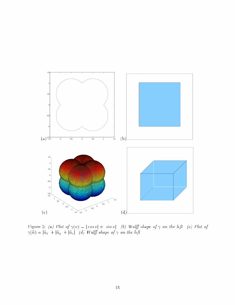
2.4 Growing a Wul� CrystalNow we consider a surprising and interesting property of objects moving outward with normalvelocity equal to the surface tension function . This is discussed in more detail in section7.3 below.In [17], Osher and Merriman proved a generalization of a conjecture made by Chernov[3, 4]. Namely, starting from any (not necessarily convex or even connected) region, if we growit with normal velocity equal to (not necessarily convex) (�) : Sd�1 ! R+, where � 2 Sd�1is the unit normal direction, the region asymptotes to a single Wul� shape correspondingto the surface tension . This is not totally surprising, because if we start with a convexregion whose support function is p(�) and move it outward with normal velocity (�), with (�) convex, the evolution of p(�; t), the support function of the growing region at time t,satis�es: � @p@t (�; t) = (�)p(�; 0) = p(�)(2.33)Thus the evolving region has support functionp(�; t) = p(�) + t (�);so the growing region asymptotes to the Wul� shape associated with (�). This argumentis only valid for convex initial shape and convex . In particular, it shows that a growingWul� shape under this motion just expands itself similarly, since p(�) = (�) for a convex . This is also true for a nonconvex . See [17] and section 7.3 below for more details.2.5 Typical Forms for Surface TensionFrom Wul�'s construction, we see that the crystalline form depends on the geometry ofthe polar plot of the surface tension. While Wul�'s construction is valid for an arbitrarysurface tension function, the polar plots of physically relevant surface tensions have severalcharacteristic features. These are worth noting in order to appreciate the crystalline formsin nature and also in order to formulate representative examples.A physical surface tension should have re ection symmetry, (n) = (�n). Further,it is known that modeling a crystalline material as a regular lattice of atoms with givenbonding energies between neighbors necessarily leads to a continuum limit in which thepolar plot of consists of portions of spheres (circles in 2D) passing through the origin[8]. In particular, a 2D plot consists of outward bulging circular arcs that meet at inwardpointing cusps. A simple example coming from a square lattice (X-Y) model of a 2D crystalis (�) = j sin(�)j+ j cos(�)j. The polar plot consists of four semicircular arcs arranged in aclover-leaf fashion. The cubic lattice (X-Y-Z) model of a 3D crystal is (n) = jnxj+jnyj+jnzj.Its plot in spherical coordinates consists of eight spherical pieces in a similar fashion. ItsWul� shape is a cube. See �gure 5.Physical surface tensions depend on the material temperature as well, and increasingtemperature tends to smooth out the cusps in the surface tension plot.From Wul�'s construction, we can see that each cusp in the plot will result in a faceton the crystal shape. Increasing the material temperature smoothes out the cusps, which inturn rounds out the original facets of the Wul� shape.14

(a) −1.5 −1 −0.5 0 0.5 1 1.5−1.5

−1

−0.5

0

0.5

1

1.5

(b)(c) −1.5

−1−0.5

00.5

11.5

−1.5

−1

−0.5

0

0.5

1

1.5−1.5

−1

−0.5

0

0.5

1

1.5

(d)Figure 5: (a) Plot of (�) = j cos �j + j sin �j. (b) Wul� shape of on the left. (c) Plot of (n) = jnxj+ jnyj+ jnzj. (d) Wul� shape of on the left.15

3 The Wul� Crystal Shape in 2DIn 2D, a unit vector can be represented by its angle to a horizontal axis. Many of the generalresults developed in the last section have interesting concrete expressions. Although we canobtain many of the results in this section by a simple change of variables and then applythe general results, as we did in the example above, we will see that 2D Wul� problem hasits own fascinating properties which may be missed by this \general-to-special" approach.Instead, we will use the general results as a guideline and develop the 2D theory from theground up. A comprehensive discussion of the 2D Wul� problem and related matters canbe found in the book of Gurtin [9].Choosing the angle between the outward unit normal to the horizontal axis as parameter,the 2D version of the Legendre transformations of a function � : S1 ! R+ are��(�) = inf���2<�<�+�2 � �(�)cos(� � �)�(3.1) ��(�) = sup���2<�<�+�2 [�(�) cos(� � �)](3.2)3.1 The Legendre Transformation in 2DWe brie y review some basic facts about plane curves. For convenience, we will change thenotation of the Legendre transformation in the section. Given r : S1 ! R+, a continuousfunction. Let r : S1 ! R2 be the polar plot of r, i.e. r(�) = r(�)(cos �; sin �), and denote thecurve as �. The second Legendre transformation of r is the support function of � and willbe denoted as p. One the other hand, given a positive continuous function p : S1 ! R+, its�rst Legendre transformation gives the Wul� shape and will be denoted as r.We will use s to denote the arclength parameter of �, and � the angle between r and thehorizontal x-axis. Let � = drds be the tangent vector and n be the outwards unit normal. Let� 2 [0; 2�) be the angle between n and x-axis.Then n = (cos �; sin �); � = (� sin �; cos �).The curvature of the curve � has a simple expression in term of �:� = d�ds(3.3)Recall that the support function of the curve � is de�ned asp(�) = max� fr(�) � n(�)g(3.4)Suppose the maximum is obtained at � = �(�). Di�erentiate with respect to �, we get:p0(�) = r(�) � � (�)(3.5)Note that r = (r � n)n+ (r � � )� . Combining the de�nition of p and the above equation,we get r(�) = p(�)n(�) + p0(�)� (�)(3.6)which gives us a simple way to express the curve if we know its support function.16

Di�erentiating equation ( 3.5) with respect to � givesp00(�) = 1� � p(�)(3.7)or equivalently: � = 1p(�) + p00(�)(3.8)This gives us a convenient way to express the curvature of a curve given its support function.Recall from the last section that for a positive function on S1 to be a support function,it must be convex in the sense that the polar plot of its reciprocal be convex. The curvatureof the polar plot of 1=p is easily shown to be� = p3(p + p00)(p2 + p02)3=2(3.9)Thus p is convex if and only if p+ p00 � 0.From the above results, we can �nd explicit formulae for the �rst and second Legendretransformations in 2D. Given p : S1 ! R+, its �rst Legendre transformation r(�) = p�(�) issimply: r(�) =pp2(�) + p02(�)(3.10)To determine � for a given �, let� = tan�1�p0(�)p(�)�(3.11)We have r(�) = r(�) �p(�)r(�) n(�) + p0(�)r(�) �(�)�= r(�)(cos(�+ �); sin(� + �))So � = � + tan�1�p0(�)p(�)�(3.12)which implicitly de�nes � for a given �. To ensure the inverse exists, we need@�@� = p(p + p00)p2 + p02 � 0or equivalently p(�) + p00(�) � 0(3.13)That is to say, p has to be convex. 17

On the other hand, suppose we are given r : S1 ! R+. To �nd its second Legendretransformation, i.e. its support function p, we note thatr0(�) = r0(�)n(�) + r(�)� (�)De�ne � = tan�1�r0(�)r(�)�(3.14)We have the following expression for the tangent vector at r(�)� (�) = r0(�)jr0(�)j = sin�n(�) + cos ��(�)= (� sin(� � �); cos(� � �))Thus � = � � tan�1�r0(�)r(�)�(3.15)which determines � for a given �. To ensure that the inverse exists, we require@�@� = r2 + 2jr0j2 � r00rr2 + jr0j2 = R(R +R00)R2 + jR0j2 � 0or equivalently R(�) +R00(�) � 0where R = 1r . This is equivalent to that r is polar convex.The support function is found to bep(�) = r(�) � n(�) = r(�)n(�) � n(�)= r(�) cos(� � �) = r(�) cos(�)= r2(�)pr2(�) + r02(�)and p(�) = p(�)(cos(� � �); sin(� � �))= r2(�)r2(�) + r02(�) [r(�)n(�)� r0(�)� (�)]where � is de�ned by equation (3.15).We summarize the results in this section in the following18

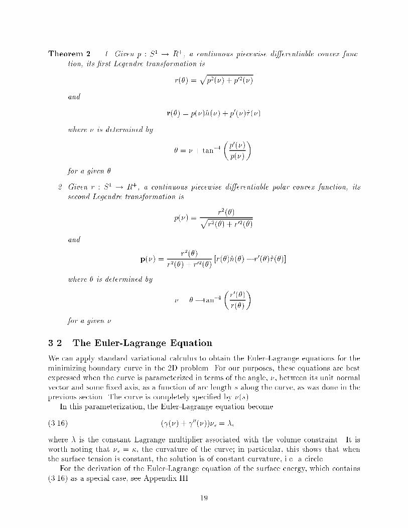
Theorem 2 1. Given p : S1 ! R+, a continuous piecewise di�erentiable convex func-tion, its �rst Legendre transformation isr(�) =pp2(�) + p02(�)and r(�) = p(�)n(�) + p0(�)� (�)where � is determined by � = � + tan�1�p0(�)p(�)�for a given �.2. Given r : S1 ! R+, a continuous piecewise di�erentiable polar convex function, itssecond Legendre transformation isp(�) = r2(�)pr2(�) + r02(�)and p(�) = r2(�)r2(�) + r02(�) [r(�)n(�)� r0(�)� (�)]where � is determined by � = � � tan�1�r0(�)r(�)�for a given �.3.2 The Euler-Lagrange EquationWe can apply standard variational calculus to obtain the Euler-Lagrange equations for theminimizing boundary curve in the 2D problem. For our purposes, these equations are bestexpressed when the curve is parameterized in terms of the angle, �, between its unit normalvector and some �xed axis, as a function of arc length s along the curve, as was done in theprevious section. The curve is completely speci�ed by �(s).In this parameterization, the Euler-Lagrange equation become( (�) + 00(�))�s = �;(3.16)where � is the constant Lagrange multiplier associated with the volume constraint. It isworth noting that �s = �, the curvature of the curve; in particular, this shows that whenthe surface tension is constant, the solution is of constant curvature, i.e. a circle.For the derivation of the Euler-Lagrange equation of the surface energy, which contains(3.16) as a special case, see Appendix III. 19

3.3 Multivalued SolutionsEquation (3.6) give us a simple ways to obtain the Wul� shape given the surface tensionfunction . We can represent the Wul� shape of using � as parameter:x(�) = (�)n(�) + 0(�)� (�)(3.17)This is true only when is convex, i.e. + 00 � 0. In this case, the curve � de�ned by x(�)is convex. When the convexity condition fails, the curve will self-intersect and thus haveswallowtails. See �gure 6. This can be easily seen by noting thatx0(�) = ( (�) + 00(�))� (�)(3.18)−2.5 −2 −1.5 −1 −0.5 0 0.5 1 1.5 2 2.5

−2.5

−2

−1.5

−1

−0.5

0

0.5

1

1.5

2

2.5

−2 −1.5 −1 −0.5 0 0.5 1 1.5 2−2

−1.5

−1

−0.5

0

0.5

1

1.5

2

Figure 6: Left: Plot of formula (3.17) when (�) = 1 + sin2(2�). Swallowtails appear sincethis is not convex. Right: Wul� shape from Wul�'s geometric construction. Notice thatby clipping o� the swallowtails in the graph on the left, we get the true Wul� shape.It is clear that the curve kinks and reverses direction whenever (�)+ 00(�) changes sign,as it does at each corner of a swallowtail. Suppose the curve x self-intersects at � = �L and� = �R, then the following condition must be satis�ed (�L)n(�L) + 0(�L)� (�L) = (�R)n(�R) + 0(�R)� (�R)(3.19)In this case, we can obtain the Wul� shape simply by clipping o� the swallowtail.There is yet another way to obtain the Wul� shape from . The Euler-Lagrange equationcan be written as a simple �rst order ordinary di�erential equation (taking � as 1, which isamounts to a rescaling of the length of the curve �)d�ds = 1( (�) + 00(�))(3.20)which completely speci�es the curve up to a scaling.20

If + 00 does not change sign, there are two possibilities. If + 00 stays positive, the righthand side is always �nite and can be integrated to compute a convex (since the curvature� = �s is positive) shape. This is the unique solution to Wul�'s problem. If + 00 � 0, andbecomes 0 at some points, the resulting curve is still convex, and yet has kinks at pointswhere + 00 vanishes.However, if + 00 does change sign, the curve one obtains from this integration willnot be convex, can have kinks (points where curvature � = �s is in�nite), and will typicallycross over itself, so that it does not even de�ne a possible material shape. The result canbe considered as a multiple valued solution to the problem, since in polar coordinates withorigin at the crystal center it corresponds to having a multivalued radius as a function ofpolar angle. This multivalued solution can be regularized to obtain the desired solution by\clipping o�" the non-physical parts of the shape created by self-crossings.3.4 Frank's Convexi�cation of Surface TensionMany di�erent surface tension functions can lead to the same Wul� shape. This is clearfrom Wul�'s geometric construction, which e�ectively ignores the behavior of the parts ofthe polar plot farthest from the origin, i.e. the high energy parts of the surface tensionfunction. Thus in general we have the freedom of using a surface tension that is equivalentto the original , in the sense that it has the same Wul� shape.The breakdown of equation (3.17) and (3.20) ultimately stems from a change in sign of + 00. We would thus like to use our freedom to de�ne an equivalent surface tension, , forwhich + 00 � 0:(3.21)It turns out there is a classical procedure known as Frank convexi�cation which yields suchan equivalent surface tension.The Frank convexi�cation of , denoted , involves two Legendre transformations andappears complicated. See formula (2.10) in section 2.3. But there exists a simple geometricprocedure to obtain from by taking the polar plot of 1= (�), forming its outer convexhull, and de�ning this to be the polar plot of 1= (�). The results in section 2.3 shows thatthe relationship between the surface tension plot and the Wul� shape becomes a standardgeometric duality when viewed under the inversion mapping. See also the article of Frank[8].Now let us take a closer look at the above procedure. The normal direction to the curver(�) = 1 (�) is � = � + tan�1� 0(�) (�)�(3.22)Thus �� = ( + 00) 2 + 02(3.23) 21

The curve fails to be convex only when + 00 < 0. There are basically two situationswhere this can happen. One situation is that there is a region on the plot of r = (�) that\bumps" out. For the plot of r = 1 (�) , it corresponds to a region that curves inward. Thusthe convexifying curve r = 1 (�) is a straight line, tangent to the curve r = 1 (�) at two points(�L; 1 (�L)) and (�R; 1 (�R)). The other situation is that the plot of r = (�) has a inward cuspat � = �M . Then the curve r = 1 (�) has a kink at � = �M , and this curve can be convexi�edby two lines which meet at the tip (�M ; 1 (�M )), and are tangent to the curve at two points(�L; 1 (�L)) and (�R; 1 (�R)). See �gure 7.1

---γ(ν )

1−−−1−−−

γ(ν )

L

R γ(ν)

1−−γ(ν )

1−−−γ(ν)

1−−γ(ν )L

R

1−−−γ(ν )MFigure 7: Left: the �rst case; Right: the second case.In the �rst case, the polar plot of contains a circular arc whose extension passes throughthe origin and (�) = (�R) sin(� � �L) + (�L) sin(�R � �)sin(�R � �L) , for �L � � � �R(3.24)One can easily derive the following jump conditions (�L) cos �L � 0(�L) sin �L = (�R) cos �R � 0(�R) sin �R(3.25) (�L) sin �L + 0(�L) cos �L = (�R) sin �R + 0(�R) cos �R(3.26)from the second order contact of the line with the original curve. Note that these equationsare exactly the self-intersection condition (3.19).In the second case, the polar plot of has two circular arcs and meet at � = �M andform a cusp there, and we have (�) = (�L) sin(�M � �) + (�M ) sin(� � �L)sin(�M � �L) , for �L � � � �M(3.27) (�) = (�M ) sin(�R � �) + (�R) sin(� � �M )sin(�R � �M ) , for �M � � � �R(3.28)At �M the convexi�ed surface tension is continuous and (�M) = (�M ), but and each have a jump in derivative there. The following inequalities are satis�ed: 0(��M ) � 0(��M ) < 0 < 0(�+M) � 0(�+M )(3.29) 22

where 0(��M ) = (�M) cos(�L � �M) � (�L)sin(�M � �L) 0(�+M ) = (�R)� (�M) cos(�L � �M)sin(�R � �M)In both cases, we have the following inequality (�) � (�); for �L � � � �R:(3.30)We note that when this convexi�ed surface tension is used within the general formula(3.17) for the multivalued solution to Wul�'s problem, the resulting curvex(�) = (�)n(�) + 0(�)� (�)(3.31)has no self-intersections and thus is the correct Wul� shape. In the �rst case discussed above, (�)+ 00(�) = 0 on [�L; �R], thus the Wul� shape de�ned by (3.31) has a sharp corner wherethe normal jumps from �L to �R. In the second case, (�) + 00(�) = 0 on [�L; �M) and(�M ; �R] and (�M) + (�M ) = 1. The normal to the Wul� shape jumps from �L to �M ,forming a corner there, then stays equal to �M and forms a facet, and then jumps againfrom �M to �R, forming another corner. Thus the second case corresponds to two cornersconnected with a facet.The Frank convexi�ed surface tension provides the basis for our general Riemann problemrepresentation of the Wul� shape.3.5 Two Formulae for the Normal DirectionRecall that the Wul� shape is given by the �rst Legendre transformation �(�) = inf���2<�<�+�2 � (�)cos(� � �)�So the problem of �nding the Wul� shape for a given is reduced to �nd the �(�) for agiven � where the in�mum is reached. This section concerns �nding explicit formulae for�(�) which we will see shortly is closely connected with the Riemann problem for a scalarconservation law.We point out some technical di�culties here. First of all, for a given �, there may existmore than one � that minimizes (�)cos(���) . This occurs partly because may not be convex.We can get rid of this di�culty by replacing by , since and have the same Wul�shape. But even if this convexity condition is satis�ed, there is still no uniqueness when (�) + 00(�) = 0. Such a situation arise at the corner of a Wul� shape. We deal with thisambiguity by requiring �(�) to be increasing and continuous from the right in �. Secondly,it is a subtle matter how to choose the range for the normal angle � and the polar angle � ofthe convex Wul� shape so that under the above assumptions on and �(�), the one to onecorrespondence between � and � is naturally de�ned. This can be achieved by choosing thehorizontal axis so that it intersects with the Wul� shape at a (global) minima of the surface23

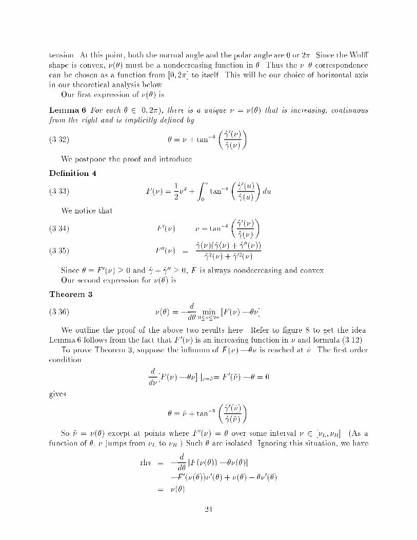
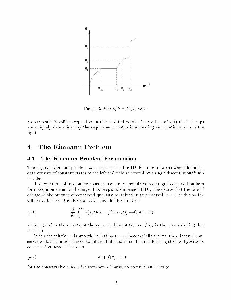
tension. At this point, both the normal angle and the polar angle are 0 or 2�. Since the Wul�shape is convex, �(�) must be a nondecreasing function in �. Thus the �{� correspondencecan be chosen as a function from [0; 2�] to itself. This will be our choice of horizontal axisin our theoretical analysis below.Our �rst expression of �(�) isLemma 6 For each � 2 [0; 2�), there is a unique � = �(�) that is increasing, continuousfrom the right and is implicitly de�ned by� = � + tan�1� 0(�) (�)�(3.32)We postpone the proof and introduceDe�nition 4 F (�) = 12�2 + Z �0 tan�1� 0(u) (u)� du(3.33)We notice that F 0(�) = � + tan�1� 0(�) (�)�(3.34) F 00(�) = (�)( (�) + 00(�)) 2(�) + 02(�)(3.35)Since � = F 0(�) � 0 and + 00 � 0, F is always nondecreasing and convex.Our second expression for �(�) isTheorem 3 �(�) = � dd� min0���2� [F (�)� ��](3.36)We outline the proof of the above two results here. Refer to �gure 8 to get the idea.Lemma 6 follows from the fact that F 0(�) is an increasing function in � and formula (3.12).To prove Theorem 3, suppose the in�mum of F (�)� �� is reached at ~�. The �rst ordercondition dd� [F (�)� ��] j�=~�= F 0(~�)� � = 0gives � = ~� + tan�1� 0(~�) (~�)�So ~� = �(�) except at points where F 0(�) = � over some interval � 2 [�L; �R]. (As afunction of �, � jumps from �L to �R.) Such � are isolated. Ignoring this situation, we haverhs = � dd� [F (�(�))� ��(�)]= �F 0(�(�))� 0(�) + �(�) + �� 0(�)= �(�) 24

θ

θ

θ

θ

1

2

3

L1ν 1Rν ν 2 ν 3

νFigure 8: Plot of � = F 0(�) vs �.So our result is valid except at countable isolated points. The values of �(�) at the jumpsare uniquely determined by the requirement that � is increasing and continuous from theright.4 The Riemann Problem4.1 The Riemann Problem FormulationThe original Riemann problem was to determine the 1D dynamics of a gas when the initialdata consists of constant states to the left and right separated by a single discontinuous jumpin value.The equations of motion for a gas are generally formulated as integral conservation lawsfor mass, momentum and energy. In one spatial dimension (1D), these state that the rate ofchange of the amount of conserved quantity contained in any interval [x1; x2] is due to thedi�erence between the ux out at x2 and the ux in at x1:ddt Z x2x1 u(x; t)dx = f(u(x2; t))� f(u(x1; t))(4.1)where u(x; t) is the density of the conserved quantity, and f(u) is the corresponding uxfunction.When the solution u is smooth, by letting x1�x2 become in�nitesimal these integral con-servation laws can be reduced to di�erential equations. The result is a system of hyperbolicconservation laws of the form ut + f(u)x = 0(4.2)for the conservative convective transport of mass, momentum and energy.25

Riemann's problem was to �nd the solution of equation (4.2) for arbitrary piecewiseconstant initial data u = uL; x < 0(4.3) u = uR; x > 0;(4.4)where uL and uR are the constant states to the left and right of the origin.The problem as posed is physically idealized, since the conservation law (4.2) does notinclude any viscous or di�usive transport e�ects. In a real gas the viscous e�ects are usuallysmall, but they do play a role when the states have steep spatial gradients as in the Riemannproblem. Indeed, it turns out that idealized Riemann problem allows multiple solutions. Theunique physically relevant one is the \viscosity solution", i.e. the limiting solution as viscositygoes to zero u = lim�#0 u� from the viscous version of the conservation law:u�t + f(u�)x = �u�xx:(4.5)In contrast, this regularized equation has unique well behaved solutions for any � > 0.Both the Riemann problem and the viscosity solution make sense for general systems ofhyperbolic conservation laws, and the names commonly refer to this more general context.The Riemann problem solutions provide insight into the fundamental propagation of discon-tinuities in the system. For our purposes, we will only need to consider a single conservationequation, so that u is a scalar state, with scalar ux f(u).A comprehensive discussion of the the Riemann problem for gas dynamics and relatedmatters can be found in the text of Courant and Friedrichs [5].4.2 Multiple-Valued SolutionsThe solutions to the Riemann problem have a simple form in which a disturbance emanatesfrom initial discontinuity at x = 0. These solutions can be found by assuming the timeself-similar form u(x; t) = u(x=t), which implies the graph of u(x; t) has the same shape atall times, di�ering only by a spatial rescaling. Substituting this form into the conservationlaw 4.2 results in the equation (�� + f 0(u))u� = 0;(4.6)where � = x=t is the similarity variable. The formal solution consists of regions on the left andright where u is constant with values uL and uR, joined by a region in which u(�) = (f 0)�1(�).If f 00(u) changes sign between uL and uR, then the inverse of f 0 is multivalued and this ucan be considered a multivalued solution of the Riemann problem.Such a multivalued solution is not physically meaningful, so some additional principle isrequired to extract a single valued solution by "clipping o�" extra values. However, from aplot of the multivalued solution it is not immediately obvious where to clip.The proper single-valued, self-similar solution to the Riemann problem is given analyti-cally by u(�) = � dd� minuL�u�uR(f(u)� �u); if uL � uR(4.7) u(�) = � dd� maxuL�u�uR(f(u)� �u); if uL � uR(4.8) 26

This formula was �rst derived by Osher in [13] and [14]; It can be understood as an analyticalinterpretation of the geometric construction given in the next section.Note that in (4.7) f can be replaced by the convexi�ed f . In the case when uL < uR, fis de�ned by f�(�) = minuL�u�uR [f(u)� �u](4.9) f(u) = max�1<�<1 [f�(�) + �u](4.10)The case uL > uR can be de�ned similarly.It follows that f(u) � f(u) if f 00(u) � 0 on the interval uL � u � uR. f is always convexand has a nondecreasing derivative.The solution to the Riemann problem at � = xt is de�ned as follows.� Case 1. There exists a unique u(�) such that f 0(u(�)) = � and f 00(u) > 0 in aneighborhood of u(�). In this case u(�) = (f 0)�1(�). This point lies in a rarefactionfan.� Case 2. f 0(u) is constant over aL � u � aR (f(u) is linear over aL � u � aR) and� = f 0(aL) = f 0(aR). In this case, the resulting solution has a jump at �: u(��) = uLand u(�+) = uR. This increasing jump in u corresponds to a contact discontinuity.� Case 3. f 0 has an increasing jump at u = u0 (f has a kink at u = u0). Thenu(�) = u0; for f 0(u�0 ) < � < f 0(u+0 ):This corresponds to a constant state.We shall show that these three situations corresponds to three scenarios in Wul� crystalshape. The rarefaction wave corresponds to regions where the angle of the normal increasessmoothly with the polar angle. The contact discontinuities correspond to the corner on aWul� crystal where the angle of the normal jumps. The constant states correspond to thefacets, where the normal to the Wul� shape points to a constant direction as the polar angleincreases.4.3 Geometric Construction of the SolutionThe general conservation law (4.2) can formally be written as the convection equation ut +v(u)ux = 0, where the convective velocity is v(u) = f 0(u). The solutions to this can bevisualized by letting each value u on the graph move horizontally with constant speed v(u).Based on this we obtain a simple geometric construction of the (possibly multiple-valued)solution to the Riemann problem. Each value from the initial step function u simply movesat its constant speed; in particular, each u value from the \step" itself, where u rangesbetween uL to uR at the single point x = 0, will propagate at its constant speed v(u). Thusthe resulting graph of u at any t > 0 will, when turned on its side, simply reproduce thegraph of v(u), u between uL and uR. This implies that u(x; t) will be a multivalued solution27

of the Riemann problem if the graph of v(u) is not monotone, i.e. if v0 = f 00 changes sign,as mentioned in the previous section.To extract the physically correct single valued solution|the viscosity solution|we applya geometric generalization of the conservation of the area under the graph of u implied by theoriginal conservation law (4.2): At each overhang in the multiple-valued graph, introduce ajump that clips o� the same amount overhanging area as it �lls in on the underhang. Referto �gure 9.u

u

L

R

x

u

Figure 9: The clipping procedure to the multivalued solution.The application of this clipping procedure to the multivalued solution at any time t > 0will yield the proper single valued, time-self similar solution. Due to the self-similarity intime, the same shape results independent of t. Note the pro�le consists of constant regions tothe far left and right, smooth regions where no clipping was necessary|\rarefactions"|andjumps where a clip was performed. These jumps in turn are classi�ed as a \contact" if thevelocity v(u) is the same on each side of the jump, or a \shock" if the velocity causes uvalues one one side to overtake those on the other. Thus values appear to ow into a shockfrom both sides as time goes by.While this clipping procedure is reasonable from the perspective of conserving u, it isnot so easy to understand why it yields the true viscosity solution, i.e. the solution selectedby the action of a small viscous dissipation.5 The 2D Wul� Crystal as the Solution of a RiemannProblemFrom the summaries of the Wul� Crystal and the Riemann problems, we can see a number ofpoints of similarity in addition to the discontinuous nature of the solutions. Both problemsadmit self-similar solutions. Both are generally formulated in terms of integral equations.Both lead to governing di�erential equations that formally have multiple-valued \solutions".In both cases the multiple-valued solutions occur due to a lack of convexity, in the sense that28

a second derivative changes sign (in the Wul� problem its the sign of + 00, in the Riemannproblem, it is f 00). And in both cases, there is a geometric construction that e�ectivelytruncates these multi valued solutions to yield the unique physical solution.With this background in place, we are prepared to discuss the precise connection anddi�erences between the two problems. There are several approaches that we can connect theWul� shape with a Riemann problem of a scalar conservation law.5.1 From the Euler-Lagrange Equation to a Scalar ConservationLaw5.1.1 The Basic ConnectionThe �rst precise formal connection comes from rewriting the Euler-Lagrange equation (3.16)fromWul�'s problem as the equation for the time self-similar solution of a Riemann problem4.6. To do this, we de�ne a function \ ux function" F (�) by the relation (assuming � = 1)F 00 = + 00(5.1)Then the Euler-Lagrange equation (3.16) can be written as(F 0(�))s = 1;(5.2)and integrating this yields (F 0(�(s))) � s = C;(5.3)where C is the constant of integration. By appropriate choice of the origin for the arclengthparameter s, we can have C = 0. In this normalization, multiplying through by �s yields(F 0(�) � s)�s = 0;(5.4)which is identical in form to the time self-similar equation (4.6). This in turn is the equationfor the Riemann problem for the conservation law�t + (F (�))x = 0:(5.5)Thus at least formally the normal angle �(s) is the time self-similar solution to a Riemannproblem for this conservation law. This would explain the crystal facets as constant states,the smooth faces as rarefactions, and the jumps in normal angle at crystal edges as shocksor contacts. However, this formal connection is not generally valid, because the di�erentialequations used in the derivation only govern smooth solutions, i.e. crystal shapes with noedges and Riemann problems with no jumps. Whether a crystal shape with edges is thesolution to this Riemann problem must be investigated separately. It turns out that theconditions at jumps are di�erent in the two problems, as described in the next subsection.Thus to completely realize the Wul� crystal as a Riemann problem solution requires a moresubtle connection. 29

5.1.2 Di�erences Between Wul� and Riemann Jump ConditionsIf the solution to a Riemann problem contains a propagating discontinuous jump, the dif-ferential equation for the conservation law (4.2) is not applicable at that point. However,the more general integral conservation law (4.1) still holds, and applied to a small intervalcontaining the jump it yields the Rankine-Hugoniot jump conditionV (u+ � u�) = f(u+)� f(u�)(5.6)where V is the constant propagation speed of the discontinuity and u+ and u� are the rightand left side values of u at the jump. This condition constrains the allowed jumps in aRiemann problem.Similarly, if a Wul� crystal has a sharp edge with a jump in normal angle �, the Euler-Lagrange equation (3.16) does not apply at that point. In this case, we can still identifya condition that governs the allowed jumps in angle. In the formal solution curve (3.17),the sharp corners on a crystal occur at points of self-intersection of the curve. These pointsseparate the primary crystal shape from the arti�cial \swallowtail" shaped appendages thatmust be removed. Thus the jump condition at the edge is simply the condition for selfintersection of this curve at two distinct normal angles �L and �R (corresponding to thenormal direction on either side of the edge): x(�L) = x(�R), or by the formula (3.17) (�L)n(�L) + 0(�L)� (�L) = (�R)n(�R) + 0(�R)� (�R):(5.7)Taking the two components of this vector condition yields two scalar jump conditions.If we compare the jump conditions for the speci�c Riemann problem (5.5) we formallyassociated with the Wul� crystal (i.e. f = F from (5.1)), and the jump conditions (5.7) thathold for the true Wul� shape, it turns out they are di�erent. The former has one constraintwhile the latter has two, and in addition, they allow di�erent jumps. As we will see, theadditional constraint comes from the fact that the allowed jumps is a contact discontinuityand must satisfy f 0(uL) = f 0(uR) = f(uR)� f(uL)uR � uL(5.8)One can easily check that the ux F de�ned above does not possess this property at thecorner.This di�erence in jump conditions means that the discontinuous physical solutions tothe Riemann problem (5.5) for �(s) do not yield the correct normal angle function for Wul�shape. Thus for crystals with corners, a more careful construction is required to realize themas the solution to a Riemann problem.The origin of this di�erence for discontinuous solutions can be traced back to the viscosityregularization used to de�ne the unique solution of Riemann problem for conservation law(4.2). Evidently, this is not the proper regularization technique for use on the Euler-Lagrangedi�erential equations for the Wul� problem. In retrospect this is not so surprising, since aproper regularizing correction for these equations should be derived by adding a physicallyreasonable energy penalty term to the original crystal energy (2.1), and using the variationalcalculus to derive the corresponding additional term in the Euler-Lagrange equations. Theproper form of such a regularizing energy correction is considered in Gurtin's book [9].30

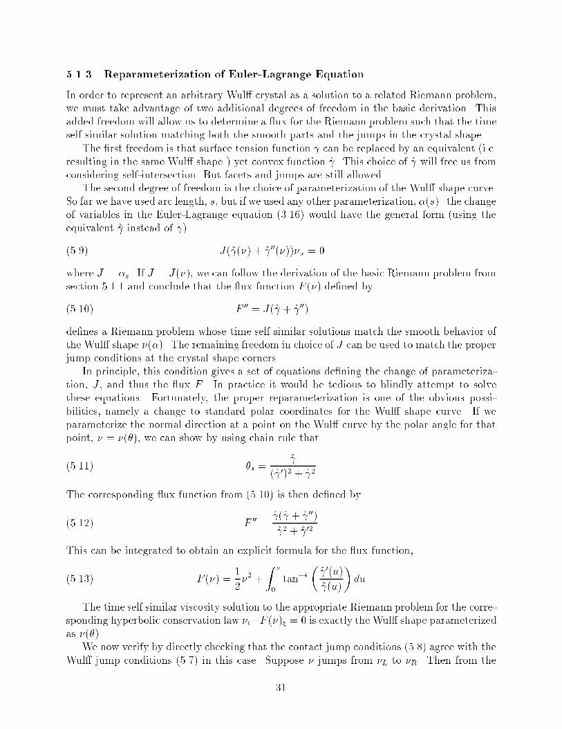
5.1.3 Reparameterization of Euler-Lagrange EquationIn order to represent an arbitrary Wul� crystal as a solution to a related Riemann problem,we must take advantage of two additional degrees of freedom in the basic derivation. Thisadded freedom will allow us to determine a ux for the Riemann problem such that the timeself similar solution matching both the smooth parts and the jumps in the crystal shape.The �rst freedom is that surface tension function can be replaced by an equivalent (i.e.resulting in the same Wul� shape ) yet convex function . This choice of will free us fromconsidering self-intersection. But facets and jumps are still allowed.The second degree of freedom is the choice of parameterization of the Wul� shape curve.So far we have used arc length, s, but if we used any other parameterization, �(s). the changeof variables in the Euler-Lagrange equation (3.16) would have the general form (using theequivalent instead of ) J( (�) + 00(�))�� = 0(5.9)where J = �s. If J = J(�), we can follow the derivation of the basic Riemann problem fromsection 5.1.1 and conclude that the ux function F (�) de�ned byF 00 = J( + 00)(5.10)de�nes a Riemann problem whose time self similar solutions match the smooth behavior ofthe Wul� shape �(�). The remaining freedom in choice of J can be used to match the properjump conditions at the crystal shape corners.In principle, this condition gives a set of equations de�ning the change of parameteriza-tion, J , and thus the ux F . In practice it would be tedious to blindly attempt to solvethese equations. Fortunately, the proper reparameterization is one of the obvious possi-bilities, namely a change to standard polar coordinates for the Wul� shape curve. If weparameterize the normal direction at a point on the Wul� curve by the polar angle for thatpoint, � = �(�), we can show by using chain rule that�s = ( 0)2 + 2(5.11)The corresponding ux function from (5.10) is then de�ned byF 00 = ( + 00) 2 + 02(5.12)This can be integrated to obtain an explicit formula for the ux function,F (�) = 12�2 + Z �0 tan�1� 0(u) (u)� du(5.13)The time self similar viscosity solution to the appropriate Riemann problem for the corre-sponding hyperbolic conservation law �t+F (�)� = 0 is exactly the Wul� shape parameterizedas �(�).We now verify by directly checking that the contact jump conditions (5.8) agree with theWul� jump conditions (5.7) in this case. Suppose � jumps from �L to �R. Then from the31

discussion in section 4.2, (�)+ 00(�) � 0 for �L � � � �R and F is linear over this interval.Note that � = F 0(�) = � + tan�1� 0(�) (�)�So the �rst equality in contact jump condition (5.8) means�L = �RThe conclusion follows from (3.24) in section 3.4.In retrospect, the correct form of ux is also the most natural one if we write the corre-sponding conservation law as @�@t + F 0(�)@�@� = 0(5.14)whose characteristic equations are � d�dt = �(�)d�dt = 0(5.15)which simply say that � is constant along the ray emanating from the origin with polar angle� = �=t . This is obviously true for the self-similar growth of Wul� crystal shape.5.2 Self-Similar Growth of Wul� Shape and Riemann ProblemIn section 2.3, we have seen that Wul� shape growing with the normal velocity equal to itssurface tension is a simple self-similar dilation. We now try to �nd the evolution equationthat governs the normal angle. We assume is convex in this section. Otherwise just replace with its Frank convexi�cation .To start with, choose the x-axis so that it intersects with Wul� shape at a minima of thesurface energy. From Wul�'s construction, the normal at this point and the x-axis coincide.Since the growth is self similar, this point will remain on the x-axis. As before, let � bethe normal angle to the positive x-axis. and s the arclength parameter. In Appendix II, wederive the evolution equation of � to be@�@t + Z �0 [ (u) + 00(u)] du@�@s = 0(5.16)If we let F 00(�) = (�) + 00(�), then the above equation becomes@�@t + F (�)@s = 0(5.17)This is the same as (5.5) which we derived above.Note that using the arclength s as a parameter is not a good choice, because for a selfsimilar growth, the point on the interface that moves on a straight line away from the origincorresponds to di�erent values of s at di�erent time. This issue actually predicts a problem32

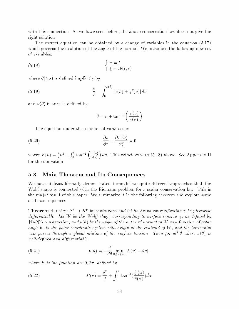
with this connection. As we have seen before, the above conservation law does not give theright solution.The correct equation can be obtained by a change of variables in the equation (5.17)which governs the evolution of the angle of the normal. We introduce the following new setof variables: � � = t� = t�(t; s)(5.18)where �(t; s) is de�ned implicitly by:st = Z �(�)0 [ (�) + 00(�)] d�(5.19)and �(�) in turn is de�ned by � = � + tan�1� 0(�) (�)�The equation under this new set of variables is@�@� + @F (�)@� = 0(5.20)where F (�) = 12�2 + R �0 tan�1 � 0(u) (u) � du. This coincides with (5.13) above. See Appendix IIfor the derivation.5.3 Main Theorem and Its ConsequencesWe have at least formally demonstrated through two quite di�erent approaches that theWul� shape is connected with the Riemann problem for a scalar conservation law. This isthe major result of this paper. We summarize it in the following theorem and explore someof its consequences.Theorem 4 Let : S1 ! R+ be continuous and let its Frank convexi�cation be piecewisedi�erentiable. Let W be the Wul� shape corresponding to surface tension , as de�ned byWul�'s construction, and �(�) be the angle of the outward normal toW as a function of polarangle �, in the polar coordinate system with origin at the centroid of W , and the horizontalaxis passes through a global minima of the surface tension. Then for all � where �(�) iswell-de�ned and di�erentiable �(�) = � dd� min0���2�[F (�)� ��];(5.21)where F is the function on [0; 2�] de�ned byF (�) = �22 + Z �0 tan�1( 0(�) (�) )d�:(5.22) 33

Furthermore, �(�; t) � �( �t ) is the time self-similar viscosity solution to the Riemann problem�t + (F (�))� = 0(5.23) �(� < 0; t = 0) = 0(5.24) �(� > 0; t = 0) = 2�:(5.25)The proof follows from Theorem 3 and Osher's formula (4.7) for the Riemann problemfor a scalar conservation law.This theorem serves as a bridge that connect the world of gas dynamics, which has a longhistory and has been extensively studied (See the book by Courant and Friedrich [5]) withthe fascinating world of crystal shapes which is characterized by facets, edges and corners.We can characterize these shapes in term of the ux F , which is a convex function. Thefacet corresponds to a kink in the graph of F in R2, which in turn corresponds to constantstates in the world of gas dynamics; The corner corresponds to a piece of a straight linein the graph of F , which in the world of gas dynamics corresponds to contact jumps; Weobserve rounded edges when a crystal melts, and the sharp corners become smooth out.These regions correspond to the smooth region in the graph of F , and, in the conservationlaw analogue, they correspond to rarefaction waves.We can also characterize these phenomena with the polar plot of . Here the facetscorrespond to cusps, and the corners correspond to circular arcs in the polar plot of .Conceptually, we have fully clari�ed the initial intuitive similarity between these disparateproblems: at least in 2D, it is completely accurate to say that the corners on a crystal arecontact discontinuities, the smooth faces are rarefactions, the facets are constant states, fora generally discontinuous solution of a hyperbolic conservation law.5.4 A Convex ExampleWe consider the surface tension (�) = j cos(�)j+ j sin(�)j:(5.26)This is an important example, since this surface tension arises in the continuum limit of thesimple X-Y lattice model of a crystal. However, it is also quite simple to analyze. We willalso remark on how it relates to the general case where appropriate.Note that the key measure of convexity, + 00, vanishes almost everywhere, but doesnot change sign. In fact, as a distribution it is (�) + 00(�) = 3Xk=0 �(� � k�2 )(5.27) � 0:(5.28)Because this quantity appears in the Euler-Lagrange equation (3.16) and in the generalizedsolution (3.17), these are both degenerate. The solution curve x(�) = (�)n(�) + 0(�)� (�)34

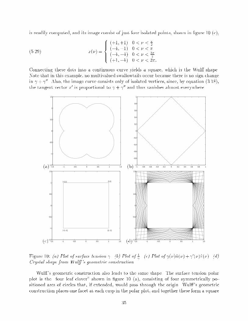
is readily computed, and its image consist of just four isolated points, shown in �gure 10 (c),x(�) = 8>><>>: (+1;+1) 0 < � < �2(�1;+1) 0 < � < �(�1;�1) 0 < � < 3�2(+1;�1) 0 < � < 2�:(5.29)Connecting these dots into a continuous curve yields a square, which is the Wul� shape.Note that in this example, no multivalued swallowtails occur because there is no sign changein + 00. Also, the image curve consists only of isolated vertices, since, by equation (3.18),the tangent vector x0 is proportional to + 00 and thus vanishes almost everywhere.(a) −1.5 −1 −0.5 0 0.5 1 1.5

−1.5

−1

−0.5

0

0.5

1

1.5

(b) −1 −0.8 −0.6 −0.4 −0.2 0 0.2 0.4 0.6 0.8 1−1

−0.8

−0.6

−0.4

−0.2

0

0.2

0.4

0.6

0.8

1

(c) −1.5 −1 −0.5 0 0.5 1 1.5−1.5

−1

−0.5

0

0.5

1

1.5

(1,−1)

(1,1)(−1,1)

(−1,−1) (d) −1.5 −1 −0.5 0 0.5 1 1.5−1.5

−1

−0.5

0

0.5

1

1.5

Figure 10: (a) Plot of surface tension . (b) Plot of 1 . (c) Plot of (�)n(�)+ 0(�)� (�). (d)Crystal shape from Wul�'s geometric construction.Wul�'s geometric construction also leads to the same shape. The surface tension polarplot is the \four leaf clover" shown in �gure 10 (a), consisting of four symmetrically po-sitioned arcs of circles that, if extended, would pass through the origin. Wul�'s geometricconstruction places one facet at each cusp in the polar plot, and together these form a square35

as shown in �gure 10 (d). The virtual facets placed at all other points along the polar plotlie entirely outside this square, and so the inner envelope de�ning the Wul� shape is thesquare itself. The simplicity of the the construction is due to the fact that the polar plot iscomposed of circular arcs; these are always \dual" to a single vertex in a polygonal Wul�shape (refer to [8] for the general properties of this duality).Next we consider the details of the Riemann problem construction. The �rst step is tocompute the ux function (5.13). Recall the that the ux function is based on the Frankconvexi�ed surface tension, . However, the surface tension function in this example isalready \convex", in the appropriate sense, i.e. + 00 � 0. Thus = , and this is a majorsource of simpli�cation over the general surface tension case. Note that in general the Frankconvexi�ed surface tension will replace any nonconvex portion of the polar plot (i.e. segmentwhere + 00 < 0 with the arc of a circle passing through the origin, since that is the curveof neutral convexity (i.e. with + 00 = 0. Because of this, the surface tension used in thisexample is representative of what generally occurs after convexi�cation.To compute the ux function, it greatly simpli�es the trigonometry to note that (�) = p2 cos(� � �(�))(5.30)where the phase shift �(�) is�(�) = �4 (2k � 1); (k � 1)�2 < � < k�2 ;(5.31)or, more succinctly, �(�) = �4 (2[ ��=2]� 1);(5.32)where [x] denotes the least integer � x.From this we get that 0 = tan(�� + �(�));(5.33)or, tan�1( 0 ) = �� + �(�):(5.34)Applying this in the ux formula 5.13, we getF (�) = �22 + Z �0 �y + �(y)dy(5.35) = Z �0 �(y)dy(5.36) = �4 ([u]2 + (1� 2[u])([u]� u));(5.37)where u = ��=2 . The graph of F is shown in �gure 11. F can easily described by notingthat it is a piecewise linear function that linearly interpolates the values F (k �2 ) = �4k2, for36

integers k = 0; 1; 2; : : : . These values in turn lie on the parabola f(�) = �2=�. Note thatthe linear segment of the graph beginning at � = k �2 has slope (2k + 1)�4 . Considering therelation to the general surface tension case, note that the piecewise linear segments of thegraph of the ux correspond to portions of the polar plot where + 00 = 0 (or, geometrically,the surface tension polar plot is a circular arc), and that these will be present wherever thesurface tension required convexi�cation. Thus they will be a typical feature of the generalcase.0 1 2 3 4 5 6 7

0

2

4

6

8

10

12

14

Figure 11: The ux function (the solid line). The dashed line is the graph of �2=�.With the ux F in hand, we can now work out the analytic form of the Riemann problemsolution from formula (5.21). The �rst step is to �nd, for a given � in [0; 2�], the minimalvalue of F (�)� ��. Note this function is also a piecewise linear (in �) function inscribed ina parabola, and so its minimum will be at the vertex where its slope switches from negativeto positive as indicated in �gure 11. This in turn will occur where F (�) changes from havingslope less that � to slope greater than �. Call this point �min(�). It can be described preciselyas follows: if � lies between �1 = (2k � 1)�4 and �2 = (2k + 1)�4 , then the transition in theslope of F will occur at �min(�) = (k � 1)�2 , at which point the slope changes from �1 to �2.Note that for a given �, k is simply the nearest integer to ��=2 . Thus we can write�min(�) = (N( ��=2)� 1)�2 ;(5.38)where N(x) is the nearest integer to x. In particular, the minimizing argument is a piecewiseconstant function of �.Continuing to unravel the Riemann problem solution formula (5.21), we see that for � inan interval for which the minimizing argument �min(�) remains constant with value �min, wehave min0���2�(F (�)� ��) = F (�min)� ��min(5.39) 37

and thus the solution to the Riemann problem for that range of � is�(�) = � dd� min0���2�(F (�)� ��)(5.40) = � dd� (F (�min)� ��min)(5.41) = �min:(5.42)Applying this over the respective � intervals corresponding to �min = 0; �=2; �; 3�=2, weobtain the complete Riemann problem solution as�(�) = 8>>>><>>>>: 0 0 � � < �=4�=2 �=4 < � < 3�=4� 3�=4 < � < 5�=43�=2 5�=4 < � < 7�=42� 7�=4 < � � 2�:(5.43)This is precisely the angle of the normal vector (to the x-axis) as a function of polar angle� for a square shape centered at the origin. Thus the solution to the Riemann problemdescribes the square Wul� shape.Finally, we can also recover the Wul� shape via the geometric solution to the Riemannproblem. For this, we �rst graph the initial data for �(�; t), which has left and right states0 and 2� with the jump at � = 0. Then we graph v(�) = F 0(�) along the � axis. In thiscase, v(�) is the piecewise constant function with values (2k + 1)�=4 over the � intervals(k�=2; (k + 1)�=2), for k = 0; 1; 2; 3. Because of the convexity of the ux F (�), there areno overhangs in the resulting plot, i.e. it de�nes a single valued function of �(�) over the �axis. This function is the self-similar solution, �(x; t) = �(x=t). We see as before that �(�)is the same function found via the analytic solution to the Riemann problem, and thus itagain describes the square Wul� shape. Regarding the general case, note that the ux willalways be convex, since F 00 = ( + 00) 2+ 02 � 0. Thus in this geometric construction, the graphof v(�) will always result in a single valued �(�), and there will be no need for the equalarea procedure of clipping o� multivalued overhangs as described in the general geometricalgorithm for solving the Riemann problem.5.5 A Nonconvex ExampleNow let us consider the following surface tension (�) = 1 + j sin(2�)j(5.44)The Wul� shape of this is also a square. See �gure 12 (d). This surface tension isnonconvex, since (�) + 00(�) = � 1� 3 sin(2�); for � 2 [0; �2 ] [ [�; 3�2 ]1 + 3 sin(2�); for � 2 [�2 ; �] [ [3�2 ; 2�](5.45)changes sign as � goes from 0 to 2�. It turn out that its Frank convexi�cation (�) =j cos �j+ j sin(�)j, which is exactly the surface tension that we discussed in the section above.Replace by , we are back to the example in the last section. Refer to �gure 12.38

(a) −2 −1.5 −1 −0.5 0 0.5 1 1.5 2−2

−1.5

−1

−0.5

0

0.5

1

1.5

2

(b) −1 −0.8 −0.6 −0.4 −0.2 0 0.2 0.4 0.6 0.8 1−1

−0.8

−0.6

−0.4

−0.2

0

0.2

0.4

0.6

0.8

1

(c) −2.5 −2 −1.5 −1 −0.5 0 0.5 1 1.5 2 2.5−2.5

−2

−1.5

−1

−0.5

0

0.5

1

1.5

2

2.5

(d) −2 −1.5 −1 −0.5 0 0.5 1 1.5 2−2

−1.5

−1

−0.5

0

0.5

1

1.5

2

Figure 12: (a) Plot of surface tension . (b) The solid line is the plot of 1 , and the dashed lineis the plot of 1 . (c) Plot of (�)n(�) + 0(�)� (�). The self-intersection of the plot indicatesthat this is nonconvex. (d) The Wul� crystal shape from Wul�'s geometric construction.39

6 Some Comments on The Wul� Problem in HigherDimensionsWe have seen in section 2.3 that the growth of Wul� crystal shape with its (convexi�ed)surface energy is simply a self-similar dilation. Suppose we grow a crystal from a in�nitesimalinitial Wul� shape, and at time t = 1 the Wul� shape is given by W (�) = �(�), then theunit outwards normal at a certain later time satis�esn(t; tW(�)) = n(1;W(�))Denote tW(�) as �, and di�erentiate with respect to t, we getnt +W(�) � r�n = 0(6.1)where r�n is the gradient of n. Recall that W(�) = D (n), we get the following@n@t + nXk=1 @ @nk (n) @n@�k = 0(6.2)This is a system of hyperbolic equations. The question of whether this system can betransformed into a system of conservation laws through a choice of suitable variables is stillopen.At present, the relation between 3D Wul� shapes and nonlinear wave dynamics is un-clear. However, the original intuitive connection between crystals and shock waves remainscompelling in 3D, and the possibility of some such relation calls for further investigation.7 The Level Set Formulation for the Wul� ProblemThe level set method of Osher and Sethian [15] has been very successful as a computationaltool in capturing the moving interfaces, especially when the interface undergoes topologicalchanges. It is also useful for the theoretical analysis of the variational problem associatedwith Wul� crystals. We now brie y review this method and apply it to the Wul� problem.7.1 The Level Set Representation of Surface EnergySuppose is a open region inRd which may be multi-connected. Let � = @ be its boundary.We de�ne an auxiliary function � so that8<: �(x) < 0, if x 2 �(x) = 0, if x 2 ��(x) > 0, otherwise.(7.1)For example, we can choose � to be the signed distance function to the interface �. Indeed,for computational accuracy, this is the most desirable case. We call � the level set functionof �. 40

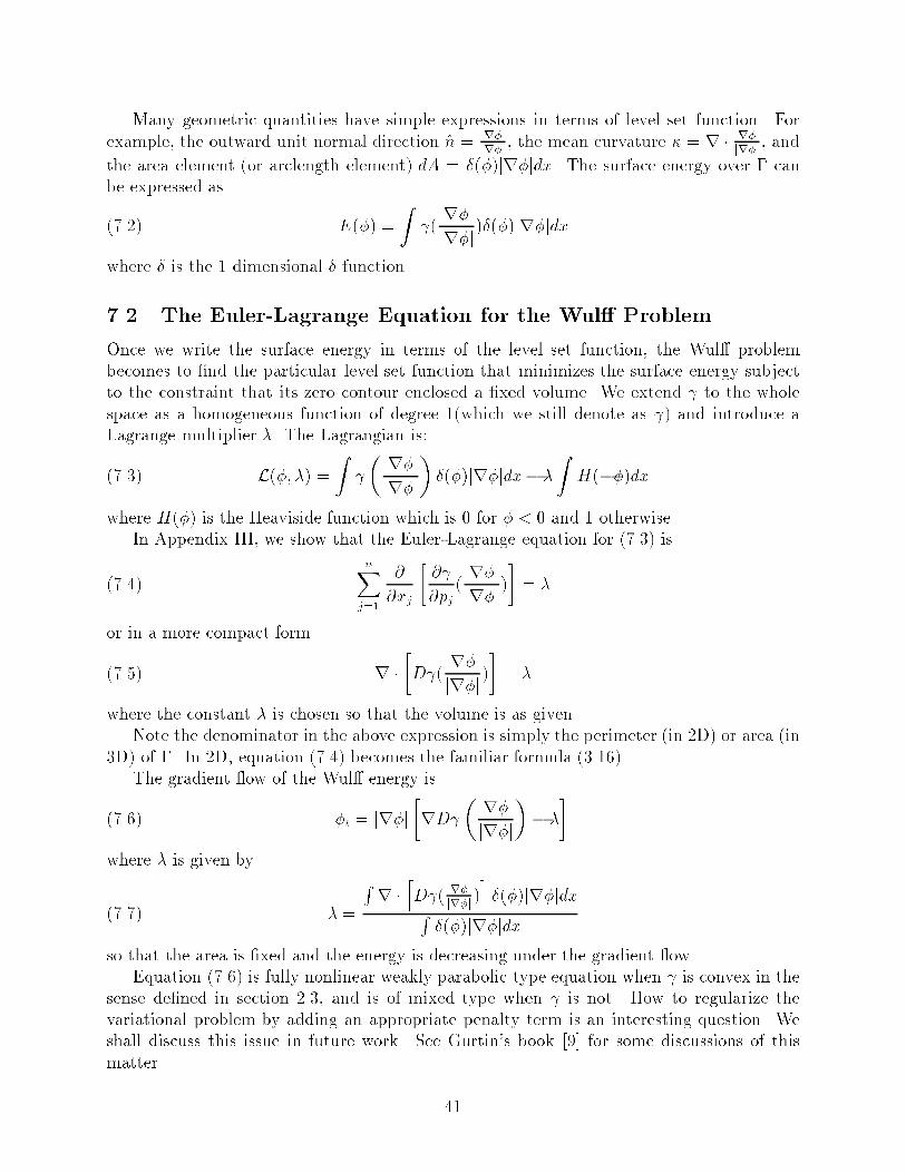
Many geometric quantities have simple expressions in terms of level set function. Forexample, the outward unit normal direction n = r�jr�j , the mean curvature � = r � r�jr�j , andthe area element (or arclength element) dA = �(�)jr�jdx. The surface energy over � canbe expressed as E(�) = Z ( r�jr�j)�(�)jr�jdx(7.2)where � is the 1 dimensional � function.7.2 The Euler-Lagrange Equation for the Wul� ProblemOnce we write the surface energy in terms of the level set function, the Wul� problembecomes to �nd the particular level set function that minimizes the surface energy subjectto the constraint that its zero contour enclosed a �xed volume. We extend to the wholespace as a homogeneous function of degree 1(which we still denote as ) and introduce aLagrange multiplier �. The Lagrangian is:L(�; �) = Z � r�jr�j� �(�)jr�jdx� �Z H(��)dx(7.3)where H(�) is the Heaviside function which is 0 for � < 0 and 1 otherwise.In Appendix III, we show that the Euler-Lagrange equation for (7.3) isnXj=1 @@xj � @ @pj ( r�jr�j)� = �(7.4)or in a more compact form r � �D ( r�jr�j)� = �(7.5)where the constant � is chosen so that the volume is as given.Note the denominator in the above expression is simply the perimeter (in 2D) or area (in3D) of �. In 2D, equation (7.4) becomes the familiar formula (3.16).The gradient ow of the Wul� energy is�t = jr�j �rD � r�jr�j�� ��(7.6)where � is given by � = R r � hD ( r�jr�j )i �(�)jr�jdxR �(�)jr�jdx(7.7)so that the area is �xed and the energy is decreasing under the gradient ow.Equation (7.6) is fully nonlinear weakly parabolic type equation when is convex in thesense de�ned in section 2.3, and is of mixed type when is not. How to regularize thevariational problem by adding an appropriate penalty term is an interesting question. Weshall discuss this issue in future work. See Gurtin's book [9] for some discussions of thismatter. 41

7.3 The Hamilton-Jacobi Equation for a Growing Wul� CrystalNow let the interface move with normal velocity equal to V , which might depend on somelocal and global properties of the interface �. Denote the boundary at a later time t as�(t), and the associated level set function as �(t; x). Let x(t) be a particle trajectory on theinterface. By de�nition, �(t; x(t)) = 0. By di�erentiating with respect to t, and noting thatV = _x(t) � r�(x)jr�(x)j, we get �t + V jr�j = 0(7.8)This is a Hamilton-Jacobi equation if V depends only on x; t; and r�. The location of theinterface is �nd by solving this equation and then �nding its zero level set fx : �(t; x) = 0g.Thus a vast wealth of recent extensive theoretical and numerical research on Hamilton-Jacobiequations can be applied to the moving interface problem.It was shown in [17] that Wul� shape growing with normal velocity equal to surfacetension is a self-similar dilation. For any other shape (which may be multiply connected),one can place two concentric Wul� shapes, such that one is contained by this shape, and theother contains this shape, and then let them grow with surface tension. Since the arbitraryshape will always be con�ned between the two Wul� shapes by the comparison principlefor the viscosity solutions to Hamilton-Jacobi equations, one immediately concludes thatthe asymptotic shape growing from any initial con�guration is a Wul� crystal shape. Fordetails of the proof with error bounds, see the recent paper [17] by Osher and Merriman.This approach give us a very convenient way to �nd the Wul� shape numerically for a givensurface energy, especially in 3D. The next section contains many examples demonstratingthis.By embedding the interface problem into a one dimensional higher space, it appears thata substantial increase in computation cost is incurred. This is not true, because we are onlyinterested in the behavior of the zero level set. A localized method can be used to lowerthe computational expense. This is discussed in [1, 23] and a more recent paper [18]. Themethod in [18] is the one that we used in our numerical examples below.8 Numerical ExamplesWe present in this section some numerical results obtained by solving equation (7.8) withV = r�jr�j , that is, �t + ( r�jr�j)jr�j = 0; x 2 Rd; t > 0(8.1)with a fast localized level set method coupled with a PDE based re-initialization step devel-oped in [18] using the ENO [16] or WENO [12] schemes for Hamilton-Jacobian equations.First, let us brie y review the numerical schemes that we shall use below for a generalHamilton-Jacobi equation: �t +H(r�) = 0; x 2 Rd; t > 0(8.2) 42

To simplify notation, we will only write down the formulae for the 2D case. The extensionto higher dimensions is straightforward.The semi-discrete version of (8.2) in 2D is:@�ij@t = �H(�+x;ij; ��x;ij; �+y;ij; ��y;ij)(8.3)where ��x;ij and ��y;ij are one-sided approximations to the partial derivatives �x and �y at(xi; yj), respectively. H is a numerical Hamiltonian that is monotone and consistent withH. See [6] or [16] for more details.In our computations, ��x;ij and ��y;ij are calculated with the 3rd order ENO scheme ofOsher and Shu [16] or the 5th order WENO scheme of Jiang and Peng [12] for Hamilton-Jacobi equations, and H is chosen as the following Lax-Friedrichs (LF) ux:HLF (u+; u�; v+; v�) = H(u+ + u�2 ; v+ + v�2 )� �2 (u+ � u�)� �2 (v+ � v�)(8.4)where � and � are arti�cial viscosities de�ned by:� = maxu2[A;B]v2[C;D] jH1(u; v)j; � = maxu2[A;B]v2[C;D] jH2(u; v)j(8.5)Here H1 = @H=@u, H2 = @H=@v, [A;B] and [C;D] are the range of u� and v�, respectively.Solutions to (8.1) often will become either too at or too steep near the interface f� = 0geven if the initial data is a perfect signed distance function. In order to avoid numericaldi�culties and retain accuracy, an additional operation, which is called re-initialization, isneeded to reset � to be a distance function again. This becomes essential for the localizedlevel set method of [18]. In [24], a PDE based re-initialization method was proposed. Bysolving the following equation:� �t + sign(�0)(jr�j � 1) = 0 in Rd �R+�(x; 0) = �0(x)(8.6)to steady state, the original level set function �0 becomes a distance function to the frontde�ned by f�0 = 0g. For (8.6), we use the Godunov numerical Hamiltonian:HGod(u+; u�; v+; v�) = � sp[max((u+)�; (u�)+)]2 + [max((v+)�; (v�)+)]2; if �0ij � 0;sp[max((u+)+; (u�)�)]2 + [max((v+)+; (v�)�)]2; otherwise.(8.7)where �0ij = �0(xi; yj), (a)+ = max(a; 0),(a)� = max(�a; 0), and s = �0=p�20 +�x is anapproximation to sign(�0).For the time discretization, we use the 3rd order TVD Runge-Kutta scheme developedin [21]. Consider the following ODE:d�dt = L(�); �(0) = �0(8.8) 43

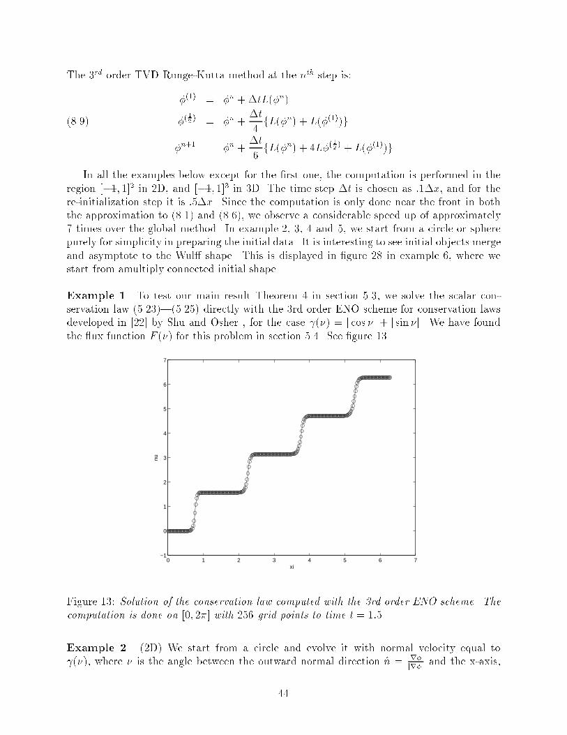
The 3rd order TVD Runge-Kutta method at the nth step is:�(1) = �n +�tL(�n)�( 12 ) = �n + �t4 fL(�n) + L(�(1))g(8.9) �n+1 = �n + �t6 fL(�n) + 4L�( 12 ) + L(�(1))gIn all the examples below except for the �rst one, the computation is performed in theregion [�1; 1]2 in 2D, and [�1; 1]3 in 3D. The time step �t is chosen as :1�x, and for there-initialization step it is :5�x. Since the computation is only done near the front in boththe approximation to (8.1) and (8.6), we observe a considerable speed up of approximately7 times over the global method. In example 2, 3, 4 and 5, we start from a circle or spherepurely for simplicity in preparing the initial data. It is interesting to see initial objects mergeand asymptote to the Wul� shape. This is displayed in �gure 28 in example 6, where westart from amultiply connected initial shape.Example 1. To test our main result Theorem 4 in section 5.3, we solve the scalar con-servation law (5.23)|(5.25) directly with the 3rd order ENO scheme for conservation lawsdeveloped in [22] by Shu and Osher , for the case (�) = j cos �j + j sin �j. We have foundthe ux function F (�) for this problem in section 5.4. See �gure 13.0 1 2 3 4 5 6 7

−1

0

1

2

3

4

5

6

7

xi

nu

Figure 13: Solution of the conservation law computed with the 3rd order ENO scheme. Thecomputation is done on [0; 2�] with 256 grid points to time t = 1:5.Example 2. (2D) We start from a circle and evolve it with normal velocity equal to (�), where � is the angle between the outward normal direction n = r�jr�j and the x-axis,44

�� � � � �. We use a 200 � 200 grid. The pictures in �gure 14{22 on the left are thecrystalline shapes obtained from Wul�'s construction, the corresponding pictures on theright are the shapes obtained from evolution. We print out the evolving shapes every 50time steps.Example 3. (3D) We start from a sphere and evolve it with normal velocity equal to (�; '), where � and ' are the spherical coordinates, �� � � � �, ��2 � ' � �2 . We usea grid of 100 � 100 � 100. We choose (�; ') = (�)hi(') for i = 1; 2 and 3. In �gure 23,h1(') = 1 + 2j sin(')j, and the corresponding Wul� shapes are prisms with di�erent basesthat depend on (�). In �gure 24, h2(') = 1+2qj sin 32('+ �2 )j, and the corresponding Wul�shapes are pyramids with di�erent bases depending on (�). h3(') = 1 + 2pj sin(j'j � �6 )j,and the corresponding Wul� shapes are bi-pyramids with various bases depending on (�).Example 4. We de�ne (n) = 1 + 2qj max1�i�20 n � vi � 1jwhere the vi's are the twenty vertices of a regular polygon of 12 faces that inscribes a unitsphere. We can expect that with the given surface intensity , the Wul� shape obtainedfromWul�'s geometric construction is a regular polygon of 12 faces, a soccer ball like object.We demonstrate this conjecture by starting with a sphere, growing it with the above de�ned . See �gure 25 for the numerical result. We use a 100� 100� 100 grid in our computation.Example 5. In this example, we study the behavior of the ratio E=V 1�1=d in the evolutionprocess. Here E = R (n)dA is surface energy, V is the volume enclosed by the surface.In a recent paper [17] of Osher and Merriman, it was shown that, starting from a convexinitial shape, this ratio decreases to its minimum as a shape grows outward normal to itselfwith velocity (�), and the decreasing is strict unless the shape is the Wul� shape. This wasproven for a general, not necessarily convex, . In the level set formulation,EV 1�1=d = R ( r�jr�j)�(�)jr�jdxR H(��)dx(8.10)where �(�) is the 1D � function, H(�) is 1D Heaviside function, d = 2 or 3 is the dimension.In our computation, �(�) is approximated by:�(�) = 8<: 0 if j�j � �,� 16�(1 + cos(�x� )) ifj�j � �2,� 16�(1 + cos(�x� )) + 43�(1 + cos(2�x� )) otherwise.(8.11)The Heaviside function H(�) is approximated by:H(�) = 8>>>><>>>>: 0 if � � ��,�16(1 + x� + 1� sin(�x� )) if � � � �2,�16(1 + x� + 1� sin(�x� )) + 13(2 + 4x� + 1� sin(2�x� )) if � � �2 ,�16(1 + x� + 1� sin(�x� )) + 43 if x � �,1 otherwise.(8.12) 45

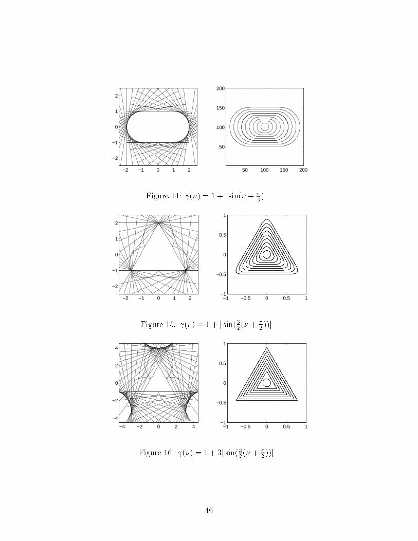
−2 −1 0 1 2

−2

−1

0

1

2

50 100 150 200

50

100

150

200

Figure 14: (�) = 1 + j sin(� + �2 )j.−2 −1 0 1 2

−2

−1

0

1

2

−1 −0.5 0 0.5 1−1

−0.5

0

0.5

1

Figure 15: (�) = 1 + j sin(32(� + �2 ))j.−4 −2 0 2 4

−4

−2

0

2

4

−1 −0.5 0 0.5 1−1

−0.5

0

0.5

1

Figure 16: (�) = 1 + 3j sin(32(� + �2 ))j.46

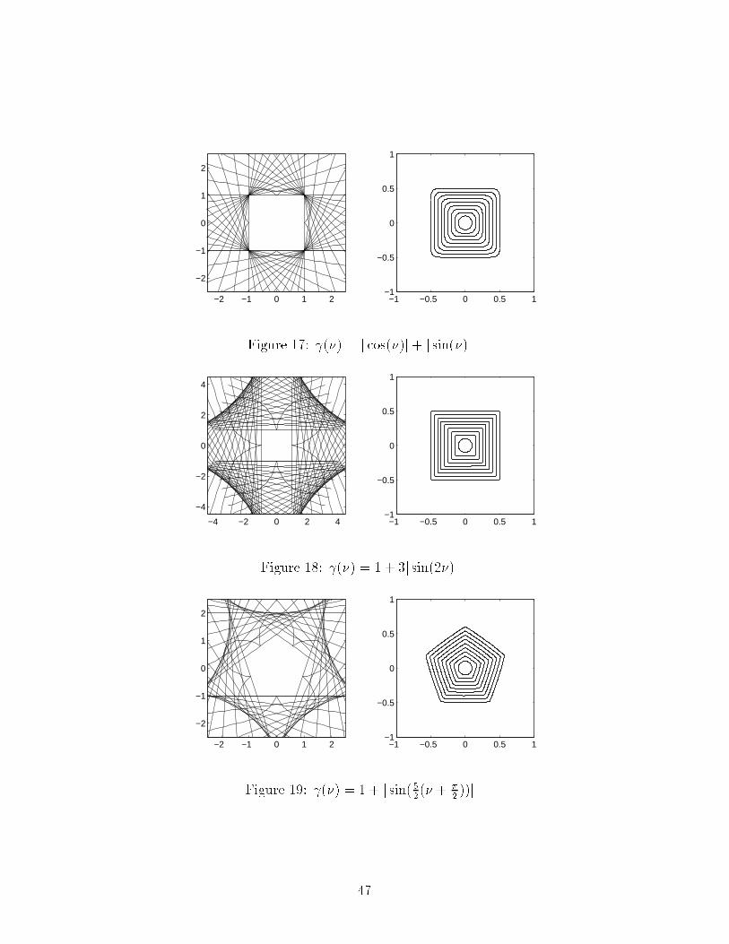
−2 −1 0 1 2

−2

−1

0

1

2

−1 −0.5 0 0.5 1−1

−0.5

0

0.5

1

Figure 17: (�) = j cos(�)j+ j sin(�)j.−4 −2 0 2 4

−4

−2

0

2

4

−1 −0.5 0 0.5 1−1

−0.5

0

0.5

1

Figure 18: (�) = 1 + 3j sin(2�)j.−2 −1 0 1 2

−2

−1

0

1

2

−1 −0.5 0 0.5 1−1

−0.5

0

0.5

1

Figure 19: (�) = 1 + j sin(52(� + �2 ))j.47

−1 −0.5 0 0.5 1−1

−0.5

0

0.5

1

−2 −1 0 1 2

−2

−1

0

1

2

Figure 20: (�) = 1 + j sin(3(� + �2 ))j.−2 −1 0 1 2

−2

−1

0

1

2

−1 −0.5 0 0.5 1−1

−0.5

0

0.5

1

Figure 21: (�) = 1 + j sin(72(� + �2 ))j.−2 −1 0 1 2

−2

−1

0

1

2

−1 −0.5 0 0.5 1−1

−0.5

0

0.5

1

Figure 22: (�) = 1 + j sin(4�)j.48

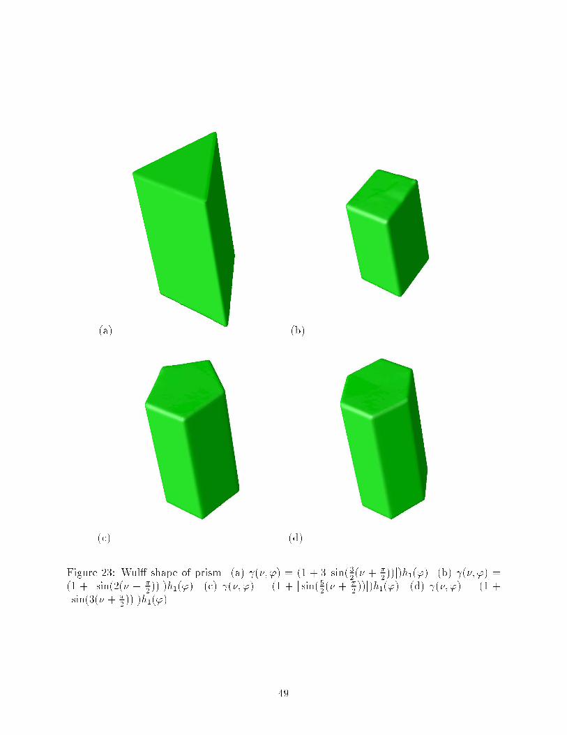
(a) (b)(c) (d)Figure 23: Wul� shape of prism. (a) (�; ') = (1 + 3j sin(32(� + �2 ))j)h1('). (b) (�; ') =(1 + j sin(2(� + �2 ))j)h1('). (c) (�; ') = (1 + j sin(52(� + �2 ))j)h1('). (d) (�; ') = (1 +j sin(3(� + �2 ))j)h1('). 49

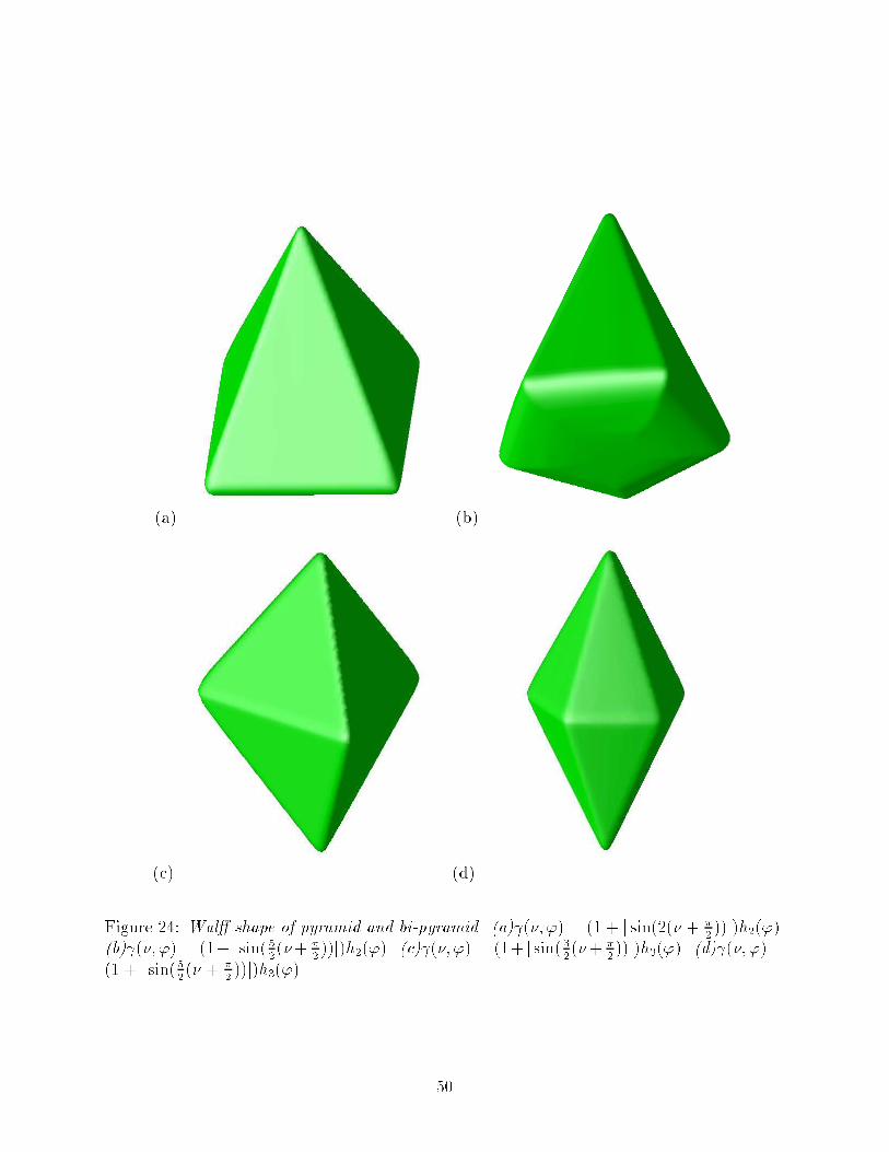
(a) (b)(c) (d)Figure 24: Wul� shape of pyramid and bi-pyramid. (a) (�; ') = (1 + j sin(2(� + �2 ))j)h2(').(b) (�; ') = (1+ j sin(52(�+ �2 ))j)h2('). (c) (�; ') = (1+ j sin(32(�+ �2 ))j)h3('). (d) (�; ') =(1 + j sin(52(� + �2 ))j)h3('). 50

Figure 25: A regular 12 polygon growed from a sphere with surface energy.where � = 3�x.We start with a circle in 2D and a sphere in 3D. As was show in [17], the ratio decreases,and is a convex function of time. If we start from a nonconvex shape, our computationsseem to show that this ratio also decreases.Example 6. In this example, we start from a nonconvex, multiply connected shape andshow how it grows, merges and �nally asymptotes to a Wul� shape. This demonstrates theversatility and simplicity of our method. See �gure 28 and 29.9 AppendixI Proof of Lemma 2In this appendix, we prove the following result stated in section 2.3.Lemma 2 is convex if and only if its homogeneous extension of degree 1 � : Rd ! R+ isa convex function on Rd.Proof: Suppose the homogeneous extension of degree 1 � : Rd ! R+ is a convex functionon Rd. Hence the region K = f x : � (x) � 1 g is convex. But K = f x : jxj ( xjxj) � 1 g =f x : jxj � 1 ( xjxj ) g which is the region enclosed by the polar plot of 1 . By de�nition, isconvex.On the other hand, suppose : Sd�1 ! R+ is convex, i.e. K = f x : jxj � �1( xjxj g isconvex. Note K = f x : jxj ( xjxj) � 1 g = f x : � (x) � 1 g since � is a degree 1 homogeneousfunction. We further conclude thatKc = f x : � (x) � c g51

0 100 200 300 4000

4

8

12

16noncovex

0 100 200 300 4000

4

8

12

16convex

Figure 26: 2D. (�) = j cos(�)j+ j sin(�)j.0 100 200 300 400

0

4

8

12

16noncovex

0 100 200 300 4000

4

8

12

16convex

Figure 27: 3D. (n) = jnxj+ jnyj+ jnzj.52

−1 0 1−1

0

10 step

−1 0 1−1

0

110 steps

−1 0 1−1

0

120 steps

−1 0 1−1

0

130 steps

−1 0 1−1

0

140 steps

−1 0 1−1

0

150 steps

−1 0 1−1

0

1100 steps

−1 0 1−1

0

1200 steps

−1 0 1−1

0

1400 steps

Figure 28: The growing and merging of the initial nonconvex and multiply connected shapeinto the Wul� shape. (�) = 1 + j sin(52(� + �2 )j.0 50 100 150 200 250 300 350 400

3

4

5

6

7

8

9

10

11

12

Figure 29: The change of energy and area ratio in the above process.53

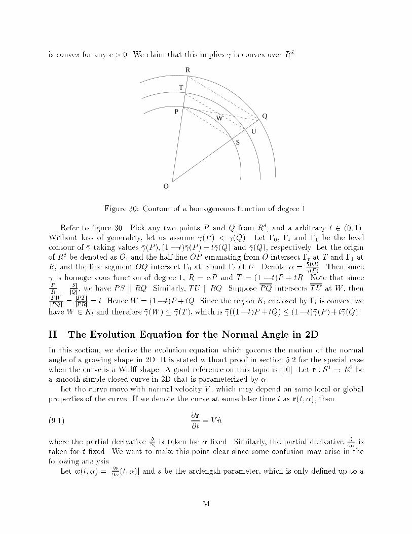
is convex for any c > 0. We claim that this implies � is convex over Rd.P

Q

O

T

R

S

U

W

Figure 30: Contour of a homogeneous function of degree 1.Refer to �gure 30. Pick any two points P and Q from Rd, and a arbitrary t 2 (0; 1).Without loss of generality, let us assume � (P ) < � (Q). Let �0, �t and �1 be the levelcontour of � taking values � (P ); (1� t)� (P ) + t� (Q) and � (Q), respectively. Let the originof Rd be denoted as O, and the half line OP emanating from O intersect �t at T and �1 atR, and the line segment �OQ intersect �0 at S and �t at U . Denote � = � (Q)� (P ) . Then since� is homogeneous function of degree 1, R = �P and T = (1 � t)P + tR. Note that sincejP jjRj = jSjjQj , we have PS k RQ. Similarly, TU k RQ. Suppose PQ intersects TU at W , thenjPW jjPQj = jPT jjPRj = t. HenceW = (1� t)P + tQ. Since the region Kt enclosed by �t is convex, wehave W 2 Kt and therefore � (W ) � � (T ), which is � ((1� t)P + tQ) � (1� t)� (P )+ t� (Q).II The Evolution Equation for the Normal Angle in 2DIn this section, we derive the evolution equation which governs the motion of the normalangle of a growing shape in 2D. It is stated without proof in section 5.2 for the special casewhen the curve is a Wul� shape. A good reference on this topic is [10]. Let r : S1 ! R2 bea smooth simple closed curve in 2D that is parameterized by �.Let the curve move with normal velocity V , which may depend on some local or globalproperties of the curve. If we denote the curve at some later time t as r(t; �), then@r@t = V n(9.1)where the partial derivative @@t is taken for � �xed. Similarly, the partial derivative @@� istaken for t �xed. We want to make this point clear since some confusion may arise in thefollowing analysis.Let w(t; �) = j @r@�(t; �)j and s be the arclength parameter, which is only de�ned up to a54

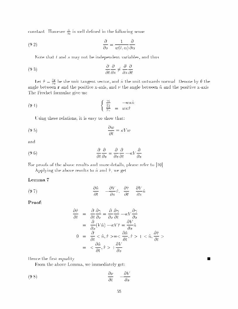
constant. However @@s is well de�ned in the following sense@@s = 1w(t; �) @@�(9.2)Note that t and s may not be independent variables, and thus@@t @@s 6= @@s @@t(9.3)Let � = @r@s be the unit tangent vector, and n the unit outwards normal. Denote by � theangle between r and the positive x-axis, and � the angle between n and the positive x-axis.The Frechet formulae give us: � @�@� = �w�n@n@� = w��(9.4)Using these relations, it is easy to show that:@w@t = �V w(9.5)and @@t @@s = @@s @@t � �V @@s(9.6)For proofs of the above results and more details, please refer to [10].Applying the above results to n and � , we getLemma 7 @n@t = �@V@s � ; @�@t = @V@s n(9.7)Proof: @�@t = @@t @ @s = @@s @ @t � �V @ @s= @@s(V n)� �V � = @V@s n0 = @@t < n; � >=< @n@t ; � > + < n; @�@t >= < @n@t ; � > +@V@sHence the �rst equality.From the above Lemma, we immediately get:@�@t = �@V@s(9.8) 55

Now we introduce the time/arclength coordinate system:� � = ts = s(t; �) = R �0 w(t; �)d�(9.9)In the this system, we have @�@t = @�@� + @�@s @s@t@s@t = Z �0 @w@t d� = Z �0 �V wd�= Z s0 V �ds = Z ��0 V d�where �0 is the normal angle of the reference point with � = 0. Note that@V@s = @V@� @�@sWe thus obtain the evolution equation for � in this system:@�@� + �Z ��0 V (�)d� + @V@� � @�@s = 0(9.10)In the self-similar growth of Wul� crystals, the velocity V = (�) and we can choose thereference point so that �0 � 0 and 0(0) = 0. We replace � by t and get@�@t + Z �0 [ (u) + 00(u)] du@�@s = 0(9.11)This conservation law gives incorrect jump conditions at corners. The correct equationcan be obtained by a change of variables in the equation (9.11) that governing the evolutionof normal angle. We introduce the following new set of variables:� � = t� = t�(t; s)(9.12)where �(t; s) is de�ned implicitly by:st = Z �0 pW 2(�) +W 02(�) d� = Z �(�)0 [ (�) + 00(�)] d�(9.13)and �(�) in turn is de�ned by � = � + tan�1� 0(�) (�)�where W (�) = �(�). 56

By the chain rule, we have @�@t = @�@� + @�@� @�@t@�@s = @�@� @�@s@�@t = � + t@�@t@�@s = t@�@sWe have the following @�@t = � st2 (�) 2(�) + 02(�)@�@s = 1t (�) 2(�) + 02(�)and thus @�@t = @�@� + @�@� �� � st (�) 2(�) + 02(�)�@�@s = @�@� (�) 2(�) + 02(�)Inserting these expression into equation (9.11), we get@�@� + @F (�)@� = 0where F (�) = �22 + R �0 tan�1 0(u) (u) du.III The Euler-Lagrange Equation of Surface EnergyThe Lagrangian (7.3) when is a homogeneous function of degree 1 is of the following formL(�; �) = Z (r�)�(�)jr�jdx� �Z H(��)dx(9.14)57

Take 2 C10 , we have< �L�� ; > def= lim�!0 1� [L(�+ � ; �)�L(�; �)]= Z fD (r�) � r �(�) + (r�)�0(�) + �(��) gdx= Z f�r � [�(�)D (r)] + (r�)�0(�) + ��(�)g dx= Z f��0(�)r �D (r�)� �(�)r �D (r) + (r�)�0(�)� ��(�)g= �Z fr �D (r�)� �g�(�) dx= �Z fr �D (r�)� �g jr�j�(�)jr�jdxHence the Euler-Lagrange equation isr �D (r�) = �(9.15)where the Lagrange constant � is chosen such that the volume enclosed is as given.Noting that when is a homogeneous function of degree 1, then D is homogeneous ofdegree 0 and hence (r�) = ( r�jr�j).For extensions of which are not necessarily homogeneous of degree 1, the Euler-Lagrangeequation can be obtained through a similar but more involved calculation and is found to ber � [ (n) +rn (n)� (rn (n) � n)n] = 0(9.16)where n = r�jr�j is function of space variable x, and the r means gradient with respect to x,and rn means gradient with respect to the variables of (extended) .For example, if we extend to be constant in the radial direction, then rn (n) � n = 0and the Euler-Lagrange equation would ber � [ (n) +rn (n)] = 0(9.17)which is di�erent from equation (9.15). We will use the homogeneous extension of degree 1next.The gradient ow of the surface energy with the volume constraints is�t = jr�j �rD � r�jr�j�� ��where � = R r � hD ( r�jr�j )i �(�)jr�jdxR �(�)jr�jdx(9.18) 58

The reason that we have included the extra term jr�j is to make the above equation rescalinginvariant, i.e. � can be replaced by h(�) with h0 > 0 and h(0) = 0.The surface energy on the gradient ow is diminishing. To see this, letF = r �D (r�)and we have dEdt = ddt Z (r�)�(phi)dx= �Z F(F � �)�(phi)jr�jdx= �Z F(F � �)dAwhere dA = �(�)jr�jdx is area element in 3D and arclength element in 2D. Using theSchwarz inequality jZ FdAj2 � Z F2dAZ dA(9.19)one easily sees that dEdt � 0(9.20)References[1] D. Adalsteinsson and J. A. Sethian, A Fast Level Set Method for Propagating Interfaces,J. Comput. Phys., v118, pp. 269-277, 1995[2] J.W. Cahn, J. E. Taylor, and C. A. Handwerker, Evolving Crystal Forms: Frank'sCharacteristics Revisited, a chapter in Sir Charles Frank, OBE, FRS: An EightiethBirthday Tribute, eds. R. G. Chambers, J. E. Enderby, A. Keller, A. R. Lang and J.W.Steeds, published by Adam Hilger Co., Bristol, England, 1991.[3] A.A. Chernov, The Kinetics of the Growth Form of Crystals, Soviet Physics Crystallog-raphy, v7 (1963), pp.728-730, translated from Krystallogra�ya, v7 (1962) pp. 895-898.[4] A.A. Chernov, Modern Crystallography III, Crystall Growth, Springer-Verlag, Berlin(1984).[5] R. Courant and K.-O. Friedrichs, Supersonic Flow and Shock Waves, Wiley, Inter-science, 1962.[6] M.G. Crandall and P.L. Lions, Two approximations of solutions of Hamilton-Jacobiequations, Math. Comput., v43, 1984, pp. 1-19.59

[7] I. Fonseca, The Wul� Theorem Revisited, Proc. Royal Soc. London A, v432 (1991) pp.125-145[8] F.C. Frank, The Geometrical Thermodynamics of Surfaces, in Metal Surfaces: Struc-ture, Energies and Kinetics, Am. Soc. Metals, Metals Park, Ohio, 1963.[9] M. E. Gurtin, Thermomechanics of Evolving Phase Boundaries in the Plane, ClarendonPress, Oxford, 1993.[10] M. Gage and R. S. Hamilton, The Heat Equation Shrinking Convex Plane Curves, J.Di�erental Geometry, 23(1986) 69-96.[11] C. Herring, chapter in The Physics of Powder Metallurgy, edited by W. E. Kingston,McGraw-Hill Book Co., New York, 1951.[12] G. S. Jiang and D. Peng, WENO Schemes for Hamilton-Jacobi equations, UCLA CAMreport 97-29, 1997. To appear in SIAM J. Sci. Comput.[13] S. Osher, The Riemann Problem for Nonconvex Scalar Conservation Laws andHamilton-Jacobi Equations, Proc. Amer. Math. Soc., v 89, pp 641-645, 1983.[14] S. Osher, Riemann Solvers, the Entropy Condition and Di�erence Approximation. SIAMJ. Numer. Anal. 21(1984) pp217-235.[15] S. Osher and J. Sethian, Fronts propagating with curvature dependent speed: algorithmsbased on Hamilton-Jacobi formulations, J. Comput. Phys., v79, 1988, pp. 12-49.[16] S. Osher and C-W. Shu, High-order essentially non-oscillatory schemes for Hamilton-Jacobi equations, J. Numer. Anal., v28, 1991, pp. 907-922.[17] S. Osher and B. Merriman, The Wul� Shape as the Asymptotic Limit of a GrowingCrytalline Interface. Asian J. Math., v1, no. 3, pp560-571, Sept. 1997.[18] D. Peng, B. Merriman, S. Osher, H-K Zhao and M. Kang A PDE Based Fast LocalLevel Set Method. UCLA CAM Report 98-25. Submitted to J. Comp. Phys.[19] B. Riemann, �Uber die Forte anzung ebener Luftwellen von enolicher Schwingungsweite,Abhandlungen der Gessellschaft der Wissenschafter zu G�ottingen, Mathematish-Physikalische Klasse 8, v. 43, 1860.[20] S. Ruuth and B. Merriman, Convolution Generated Motion and Generalized Huygens'Principles for Interface Motion. UCLA CAM Report 98-4.[21] C-W. Shu, Total-Variation-Diminishing Time Discretization, SIAM J. Sci. Stat. Com-put. v9, pp. 1073-1084, 1988.[22] C-W. Shu and S. Osher, E�cient implementation of essentially non-oscillatory shock-capturing schemes II, J. Comput. Phys., v83, 1989, pp. 32-78.60

[23] J. A. Sethian, A Fast Marching Level Set Method for Monotonically Advancing FrontsProc. Nat. Acad. Sci., v93, 4, pp. 1591-1595, 1996.[24] M. Sussman, P. Smereka and S. Osher, A Level Set Approach for Computing Solutionsto Incompressible Two-Phase Flow, vol. 114, no. 1, Sept. 1994, pp. 146-159.[25] J. E. Taylor, Existence and Structure of Solutions to a Class of Non-elliptic VariationalProblems. Symposia Mathematica v 14, pp 499-508, 1974.[26] G. Wul�, Zur Frage der Geschwindigkeit des Wachsthums und der Au �osung der Krys-tall achen, Zeitschrift f�ur Krystallographie und Minerologie, v 34, pp 449-530, 1901.

61