arX

iv:m

ath-

ph/0

1100

42v1

31

Oct

200

1

CUQM-89

math-ph/0110042

October 2001

Closed-form sums for some perturbation series involvingassociated Laguerre polynomials

Richard L. Hall † , Nasser Saad ‡ and Attila B. von Keviczky †

† Department of Mathematics and Statistics, Concordia University,1455 de Maisonneuve Boulevard West, Montreal,

Quebec, Canada H3G 1M8.

‡ Department of Mathematics and Computer Science,University of Prince Edward Island,

550 University Avenue, Charlottetown,PEI, Canada C1A 4P3.

Abstract

Infinite series∞∑

n=1

( α2)n

n1n! 1F1(−n, γ, x2) , where 1F1(−n, γ, x2) = n!

(γ)nL

(γ−1)n (x2), appear

in the first-order perturbation correction for the wavefunction of the generalized spikedharmonic oscillator Hamiltonian H = − d2

dx2 +Bx2 + Ax2 + λ

xα 0 ≤ x <∞, α, λ > 0, A ≥ 0.

It is proved that the series is convergent for all x > 0 and 2γ > α where γ = 1 +12

√1 + 4A . Closed-form sums are presented for these series for the cases α = 2, 4, and

6 . A general formula for finding the sum for α2 = 2 + m,m = 0, 1, 2 . . . in terms of

associated Laguerre polynomials is also provided.

PACS 03.65.Ge

Closed-form sums . . . page 2

I. Introduction

Aguillera-Navarro and Guardiola [1] encounter some difficulties inherent in con-nection with attempts to derive the first-order perturbation expansion to the wave-

function of the spiked harmonic oscillator Hamiltonian

H = − d2

dx2+ x2 +

λ

xα0 ≤ x <∞, α, λ > 0, (1.1)

even for the case of α = 2 , where a complete exact solution is also available. The

reason for these difficulties lies in computing infinite series of the type

∞∑

n=1

(α2 )n

n

1

n!1F1(−n;

3

2;x2), (1.2)

where 1F1 stands for the confluent hypergeometric function defined by

1F1(−n; b; y) =

n∑

k=0

(−n)k

(b)k

yk

k!=

n!

(b)nL(b−1)

n (y) (1.3)

in terms of the associated Laguerre polynomials L(b−1)n (y), and (a)n, the shifted fac-

torial (or Pochhammer symbols) defined by

(a)0 = 1, (a)n = a(a+ 1)(a+ 2) . . . (a+ n− 1) =Γ(a+ n)

Γ(a), n = 1, 2, . . . . (1.4)

Recently, the present authors studied a more general Hamiltonian known now as

the generalized spiked harmonic oscillator Hamiltonian [2 − 5]

H = H0 + λV = − d2

dx2+Bx2 +

A

x2+

λ

xα0 ≤ x <∞, α, λ > 0, A ≥ 0, (1.5)

defined on the one-dimensional space (0 ≤ x < ∞) with eigenfunctions satisfyingDirichlet boundary conditions, that is to say, with wavefunctions vanishing at the

boundaries. Herein Eq.(1.1) appears as a special case (A = 0, B = 1 ). They found thatthe matrix elements of the operator x−α , with respect to the exact solutions of the

Gol’dman and Krivchenkov Hamiltonian H0 , namely

ψn(x) = (−1)n

√

2Bγ2 Γ(n+ γ)

n!Γ2(γ)xγ− 1

2 e−√

B2

x2

1F1(−n, γ,√Bx2), (1.6)

with exact eigenenergies

En = 2√B(2n+ γ), n = 0, 1, 2, . . . , γ = 1 +

1

2

√1 + 4A, (1.7)

are given explicitly by the following expressions:

x−αmn = (−1)n+mB

α4

(α2 )n

(γ)n

Γ(γ − α2 )

Γ(γ)

√

(γ)n(γ)m

n!m!3F2(−m, γ − α

2, 1 − α

2; γ, 1 − n− α

2; 1), (1.8)

Closed-form sums . . . page 3

and valid for all values of the parameters γ and α such that α < 2γ . Furthermore,the matrix elements of the Hamiltonian Eq.(1.5) are given by

Hmn =< m|H |n >≡ 2√B(2n+ γ)δnm + λ(−1)m+nB

α4

√

(γ)n(γ)m

n!m!

Γ(γ − α2 )(α

2 )n

(γ)nΓ(γ)

3F2(−m, γ −α

2, 1 − α

2; γ, 1 − α

2− n; 1).

(1.9)

Of particular interest are the elements

H0n = λ(−1)nBα4

√

(γ)n

n!

Γ(γ − α2 )

Γ(γ)

(α2 )n

(γ)n, n 6= 0. (1.10)

It is known that the first correction to the wavefunction by means of standard per-

turbation techniques leads to

ψ(1)0 (x) =

∞∑

n=1

H0n

E0 − Enψn(x), (1.11)

where H0n and ψn(x) are given by Eq.(1.10) and (1.6), respectively. Thus, the first

correction to the wavefunction of the Hamiltonian Eq.(1.5) is given by

ψ(1)0 (x) = −B

α2+ γ

4− 1

2

2√

2

Γ(γ − α2 )

Γ(γ)√

Γ(γ)xγ− 1

2 e−√

B2

x2

∞∑

n=1

(α2 )n

n

1

n!1F1(−n, γ,

√Bx2). (1.12)

The purpose of this article is to find closed-form sums for the infinite series appearingin Eq.(1.12), namely

∞∑

n=1

(α2 )n

n

1

n!1F1(−n; γ;x2), (1.13)

where 2γ > α , α = 2, 4, 6, . . . and we set B = 1, for simplicity. Because of Eq.(1.3), theresults of this article can be expressed equally well in terms of the associated Laguerre

polynomials. The importance of closed-form sums for the infinite series (1.13) is thatthey help us to understand the abnormal behavior of the standard, weak coupling,

perturbation theory [1] for the singular Hamiltonians (1.1). Such infinite series wereinvestigated earlier by the present authors [2] , where they prove, in the case of α < 2 ,

we have, by means of the inverse Laplace transform, that

∞∑

n=1

(α2 )n

n

1

n!1F1(−n, γ, x2) =

Γ(γ)

2πi

α

2

c+i∞∫

c−i∞

ett−γ(1− x2

t)3F2(1+

α

2, 1, 1; 2, 2; 1− x2

t)dt, c > 0, (1.14)

where |1 − x2

t | < 1 which is indeed an important condition to insure the convergence

of the series 3F2 that appears on the right-hand side of (1.14). The functions 3F2 and

1F1 , mentioned above, are special cases of the generalized hypergeometric function

pFq(α1, α2, . . . , αp;β1, β2, . . . , βq; z) =

∞∑

k=0

p∏

i=1

(αi)k

q∏

j=1

(βj)k

zk

k!, (1.15)

Closed-form sums . . . page 4

where p and q are non-negative integers and βj ( j = 1, 2, . . . , q ) none of which isequal to zero or to a negative integer. If the series does not terminate (either of αi ,

i = 1, 2, . . . , p , is negative integer), then the series converges or diverges according as|z| < 1 or |z| > 1 . For z = 1 on the other hand, the series is convergent, provided

q∑

j=1

βj −p∑

i=1

αi > 0. This paper is organized as follows: in Sec. II we demonstrate that

the infinite series on the left hand side of Eq.(1.14) converges for all x > 0 and γ > α2 .

Furthermore, the integral representaion is still valid in such cases. In Sec. III we provethat in the case α = 2 , we have

∞∑

n=1

(1)n

n n!1F1(−n; γ;x2) = ψ(γ) − log x2, γ > 1,

while in the case α = 4 , we have

∞∑

n=1

(2)n

n n!1F1(−n; γ;x2) = ψ(γ) − log x2 +

γ − 1

x2− 1, γ > 2,

and for the case α = 6

∞∑

n=1

(3)n

n n!1F1(−n; γ;x2) = ψ(γ) − log x2 +

γ − 1

x2− 3

2+

(γ − 1)(γ − 2)

2x4, γ > 3.

In Sec. IV we prove our main result that for α2 = 2 +m,m = 0, 1, 2, . . .

∞∑

n=1

(α2 )n

n n!1F1(−n; γ;x2) = ψ(γ) − log x2 − (m+ 1)

m∑

k=0

(−m)k

(k + 1)2

(

− 1

x2

)k[

Lγ−1−kk (x2)

− (γ − 1)

x2L

γ−2−kk (x2)

]

where L(a)n (·) stands for the well-known associated Laguerre polynomials. An inter-

pretation for the first-order correction of the wave function Eq.(1.12) as x → 0 and

some further remarks are given in Sec. V.

II. Integral Representation and the Convergence Problem

In order to evaluate the sum in Eq.(1.13) for α > 0 and 2γ > α , we require asuitable integral representation of the confluent hypergeometric function 1F1(−n, γ, x2)

over an appropriate contour, in order to interchange summation with integration and

thereby readily conclude the absolute convergence of the series just mentioned. Wefind the inverse Laplace transform (integral) representation [6]

1F1(a, γ, x2) =

Γ(γ)

2πi

c+i∞∫

c−i∞

ett−γ(1 − x2

t)−adt (2.1)

under the conditions Re(γ) > 0, c > 0, |arg(1− x2

c )| < π (which is clearly true for x real)to be most advantageous for achieving this end.

Closed-form sums . . . page 5

Now turn to the evaluation of the summation in terms of the representation (2.1)written for a = −n , namely

1F1(−n, γ, x2) =Γ(γ)

2πi

c+i∞∫

c−i∞

ett−γ(1 − x2

t)ndt, n = 0, 1, 2, . . . , (2.2)

which substituted into the summation of Eq.(1.13) yields

∞∑

n=1

(α2 )n

n

1

n!1F1(−n, γ, x2) = (2πi)−1Γ(γ)

∞∑

n=1

(α2 )n

n

1

n!

c+i∞∫

c−i∞

ett−γ(1 − x2

t)ndt

= (2π)−1Γ(γ)

∞∑

n=1

(α2 )n

n

1

n!

∞∫

−∞

e(c+iy)(c+ iy)−γ(1 − x2

c+ iy)ndy.

(2.3)

The evaluation of this last infinite sum, involving integrations over the interval(−∞,∞ ), is achieved by examining the summation of the integrand, namely

∞∑

n=1

(α2 )n

n

1

n!e(c+iy)(c+ iy)−γ(1 − x2

c+ iy)n = e(c+iy)(c+ iy)−γ

∞∑

n=1

(α2 )n

n

1

n!(1 − x2

c+ iy)n, (2.4)

and demonstrating that it has an L1(−∞,∞) -majorant. Hence, the existence of sucha majorant shall permit us to interchange summation with integration, as result of

the Lebesgue Dominated Convergence Theorem. To arrive at such a majorant, wecontinue by noting that

∞∑

n=1

(α2 )n

n

1

n!(1 − x2

c+ iy)n =

∞∑

n=0

(α2 )n+1

n+ 1

1

(n+ 1)!(1 − x2

c+ iy)n+1

=α

2(1 − x2

c+ iy)

∞∑

n=0

(α2 + 1)n

(2)n

(1)n

(2)n(1 − x2

c+ iy)n

=α

2(1 − x2

c+ iy)

∞∑

n=0

(α2 + 1)n(1)n(1)n

(2)n(2)n

(1 − x2

c+iy )n

n!

=α

2(1 − x2

c+ iy)3F2(

α

2+ 1, 1, 1; 2, 2; 1− x2

c+ iy)

(2.5)

as consequence of (a)n+1 = a(a+ 1)n , n! = (1)n and (n+ 1)! = (2)n . The series 3F2 , in

Eq.(2.5), is convergent provided that |1 − x2

c+iy | < 1 . Now, since

1 − x2

c+ iy= 1 − x2(c− iy)

c2 + y2= 1 − x2c

c2 + y2+ i

x2y

c2 + y2,

for which∣

∣

∣

∣

1 − x2

c+ iy

∣

∣

∣

∣

2

= 1 − x2(2c− x2)

c2 + y2< 1,

provided c is chosen large enough - i. e. x2 < 2c . For such c we shall always have

0 < 1 − x2(2c− x2)

c2 + y2< 1 ∀y ∈ R. (2.6)

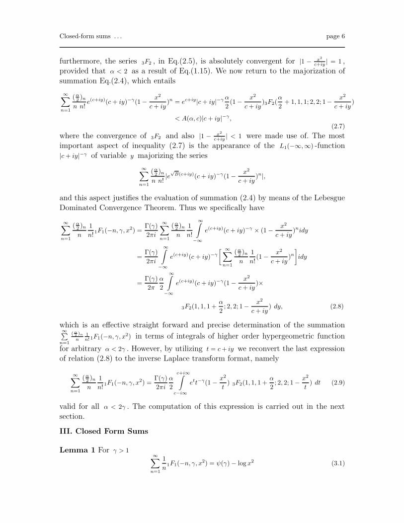
Closed-form sums . . . page 6

furthermore, the series 3F2 , in Eq.(2.5), is absolutely convergent for |1 − x2

c+iy | = 1 ,provided that α < 2 as a result of Eq.(1.15). We now return to the majorization of

summation Eq.(2.4), which entails

∞∑

n=1

(α2 )n

n n!e(c+iy)(c+ iy)−γ(1 − x2

c+ iy)n = ec+iy|c+ iy|−γ α

2(1 − x2

c+ iy)3F2(

α

2+ 1, 1, 1; 2, 2; 1− x2

c+ iy)

< A(α, c)|c+ iy|−γ ,

(2.7)

where the convergence of 3F2 and also |1 − x2

c+iy | < 1 were made use of. The mostimportant aspect of inequality (2.7) is the appearance of the L1(−∞,∞) -function

|c+ iy|−γ of variable y majorizing the series

∞∑

n=1

(α2 )n

n n!|e

√B(c+iy)(c+ iy)−γ(1 − x2

c+ iy)n|,

and this aspect justifies the evaluation of summation (2.4) by means of the Lebesgue

Dominated Convergence Theorem. Thus we specifically have

∞∑

n=1

(α2 )n

n

1

n!1F1(−n, γ, x2) =

Γ(γ)

2πi

∞∑

n=1

(α2 )n

n

1

n!

∞∫

−∞

e(c+iy)(c+ iy)−γ × (1 − x2

c+ iy)nidy

=Γ(γ)

2πi

∞∫

−∞

e(c+iy)(c+ iy)−γ

[ ∞∑

n=1

(α2 )n

n

1

n!(1 − x2

c+ iy)n

]

idy

=Γ(γ)

2π

α

2

∞∫

−∞

e(c+iy)(c+ iy)−γ(1 − x2

c+ iy)×

3F2(1, 1, 1 +α

2; 2, 2; 1− x2

c+ iy) dy, (2.8)

which is an effective straight forward and precise determination of the summation∞∑

n=1

( α2)n

n1n! 1F1(−n, γ, x2) in terms of integrals of higher order hypergeometric function

for arbitrary α < 2γ . However, by utilizing t = c+ iy we reconvert the last expressionof relation (2.8) to the inverse Laplace transform format, namely

∞∑

n=1

(α2 )n

n

1

n!1F1(−n, γ, x2) =

Γ(γ)

2πi

α

2

c+i∞∫

c−i∞

ett−γ(1 − x2

t) 3F2(1, 1, 1 +

α

2; 2, 2; 1 − x2

t) dt (2.9)

valid for all α < 2γ . The computation of this expression is carried out in the next

section.

III. Closed Form Sums

Lemma 1 For γ > 1∞∑

n=1

1

n1F1(−n, γ, x2) = ψ(γ) − log x2 (3.1)

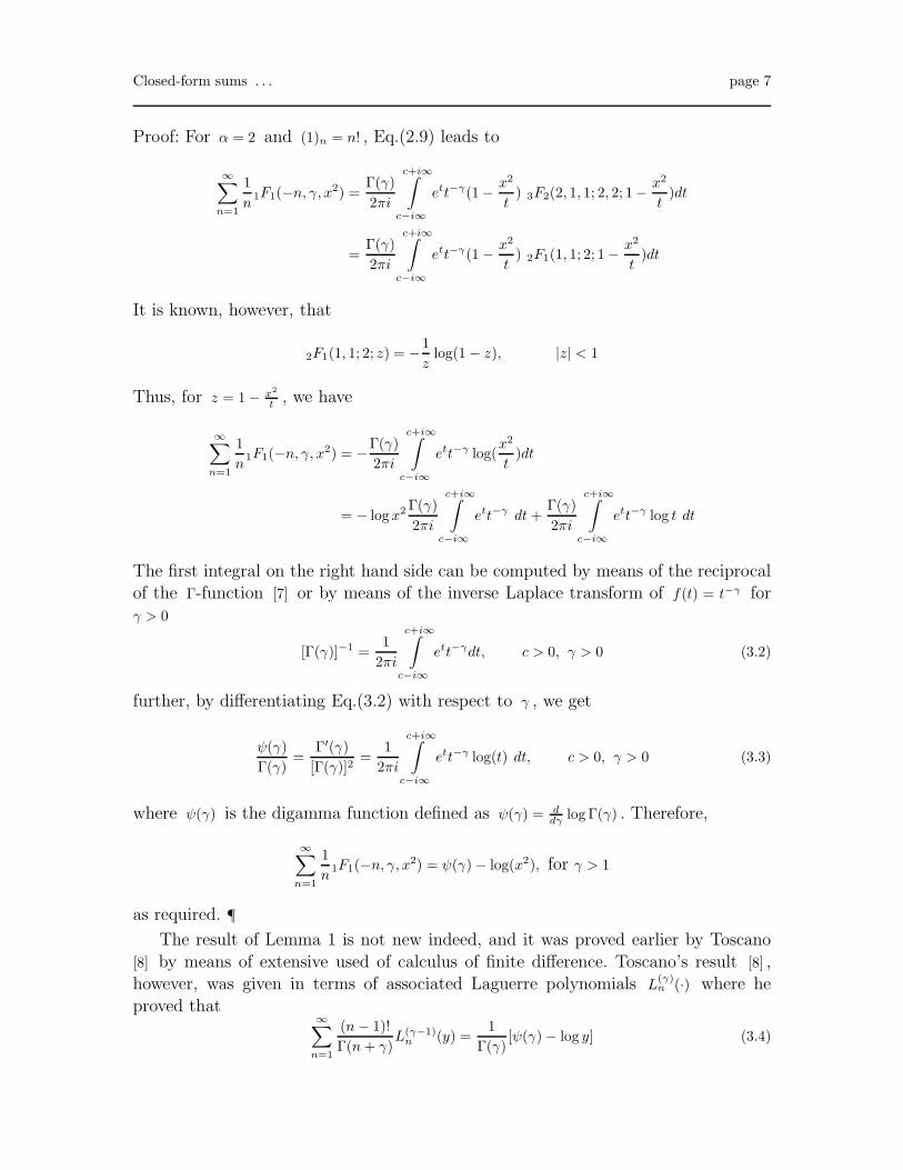
Closed-form sums . . . page 7

Proof: For α = 2 and (1)n = n! , Eq.(2.9) leads to

∞∑

n=1

1

n1F1(−n, γ, x2) =

Γ(γ)

2πi

c+i∞∫

c−i∞

ett−γ(1 − x2

t) 3F2(2, 1, 1; 2, 2; 1− x2

t)dt

=Γ(γ)

2πi

c+i∞∫

c−i∞

ett−γ(1 − x2

t) 2F1(1, 1; 2; 1 − x2

t)dt

It is known, however, that

2F1(1, 1; 2; z) = −1

zlog(1 − z), |z| < 1

Thus, for z = 1 − x2

t , we have

∞∑

n=1

1

n1F1(−n, γ, x2) = −Γ(γ)

2πi

c+i∞∫

c−i∞

ett−γ log(x2

t)dt

= − logx2 Γ(γ)

2πi

c+i∞∫

c−i∞

ett−γ dt+Γ(γ)

2πi

c+i∞∫

c−i∞

ett−γ log t dt

The first integral on the right hand side can be computed by means of the reciprocalof the Γ-function [7] or by means of the inverse Laplace transform of f(t) = t−γ for

γ > 0

[Γ(γ)]−1 =1

2πi

c+i∞∫

c−i∞

ett−γdt, c > 0, γ > 0 (3.2)

further, by differentiating Eq.(3.2) with respect to γ , we get

ψ(γ)

Γ(γ)=

Γ′(γ)

[Γ(γ)]2=

1

2πi

c+i∞∫

c−i∞

ett−γ log(t) dt, c > 0, γ > 0 (3.3)

where ψ(γ) is the digamma function defined as ψ(γ) = ddγ log Γ(γ) . Therefore,

∞∑

n=1

1

n1F1(−n, γ, x2) = ψ(γ) − log(x2), for γ > 1

as required. ¶The result of Lemma 1 is not new indeed, and it was proved earlier by Toscano

[8] by means of extensive used of calculus of finite difference. Toscano’s result [8] ,however, was given in terms of associated Laguerre polynomials L

(γ)n (·) where he

proved that∞∑

n=1

(n− 1)!

Γ(n+ γ)L(γ−1)

n (y) =1

Γ(γ)[ψ(γ) − log y] (3.4)

Closed-form sums . . . page 8

For comparison, we use the relation between the confluent hypergeometric function

1F1(−n; γ + 1; ·) and the associated Laguerre polynomials L(γ)n (·) , namely

1F1(−n, γ + 1, ·) =Γ(n+ 1)Γ(γ + 1)

Γ(n+ γ + 1)L(γ)

n (·). (3.5)

Thus,∞∑

n=1

1

n1F1(−n, γ, x2) = Γ(γ)

∞∑

n=1

(n− 1)!

Γ(n+ γ)L(γ−1)

n (x2), (3.6)

and this leads to the same results as lemma (1). In other words, Lemma (1) gives an

independent proof of Toscano’s result [8] .

In order to find closed sums for Eq.(2.8) for positive even numbers of α , we startwith the reduction formula for 3F2(a, b, 1; c, 2; z) as given by Luke [9]

z 3F2(a, b, 1; c, 2; z) =(c− 1)

(a− 1)(b− 1)

[

2F1(a− 1, b− 1; c− 1; z) − 1

]

, |z| < 1. (3.7)

The purpose of the following lemma is to find the limit of Luke’s identity as b→ 1 .

Lemma 2 For a 6= 1 , c 6= 1 , and | zz−1 | < 1 ,

z 3F2(a, 1, 1; c, 2; z) =(c− 1)

(a− 1)

[

(c− a)

(c− 1)

(

z

z − 1

)

3F2(c− a+ 1, 1, 1; c, 2;z

z − 1) − log(1 − z)

]

, (3.8)

Proof: From Pfaff’s transformation [10] for 2F1 ,

2F1(a, b; c; z) = (1 − z)−a2F1(a, c− b; c;

z

z − 1), | z

z − 1| < 1 (3.9)

which is also known as Euler’s second identity, we have, by means of Eq.(2.1), that

z 3F2(a, 1, 1; c, 2; z) = limb→1

(c− 1)

(a− 1)(b− 1)

[

(1 − z)−(b−1)2F1(c− a, b− 1; c− 1;

z

z − 1) − 1

]

Using the identity(1 − z)−(b−1) = e−(b−1) log(1−z),

and the series representation

2F1(c− a, b− 1; c− 1;z

z − 1) =

∞∑

n=0

(c− a)n(b− 1)n

(c− 1)n n!

(

z

z − 1

)n

= 1 +∞∑

n=1

(c− a)n(b− 1)n

(c− 1)n n!

(

z

z − 1

)n

we have

z 3F2(a, 1, 1; c, 2; z) = limb→1

(c− 1)

(a− 1)(b− 1)

[{

1 − (b− 1) log(1 − z) +1

2(b− 1)2[log(1 − z)]2

+O(b − 1)3}{

1 +

∞∑

n=1

(c− a)n(b − 1)n

(c− 1)n n!

(

z

z − 1

)n}

− 1

]

.

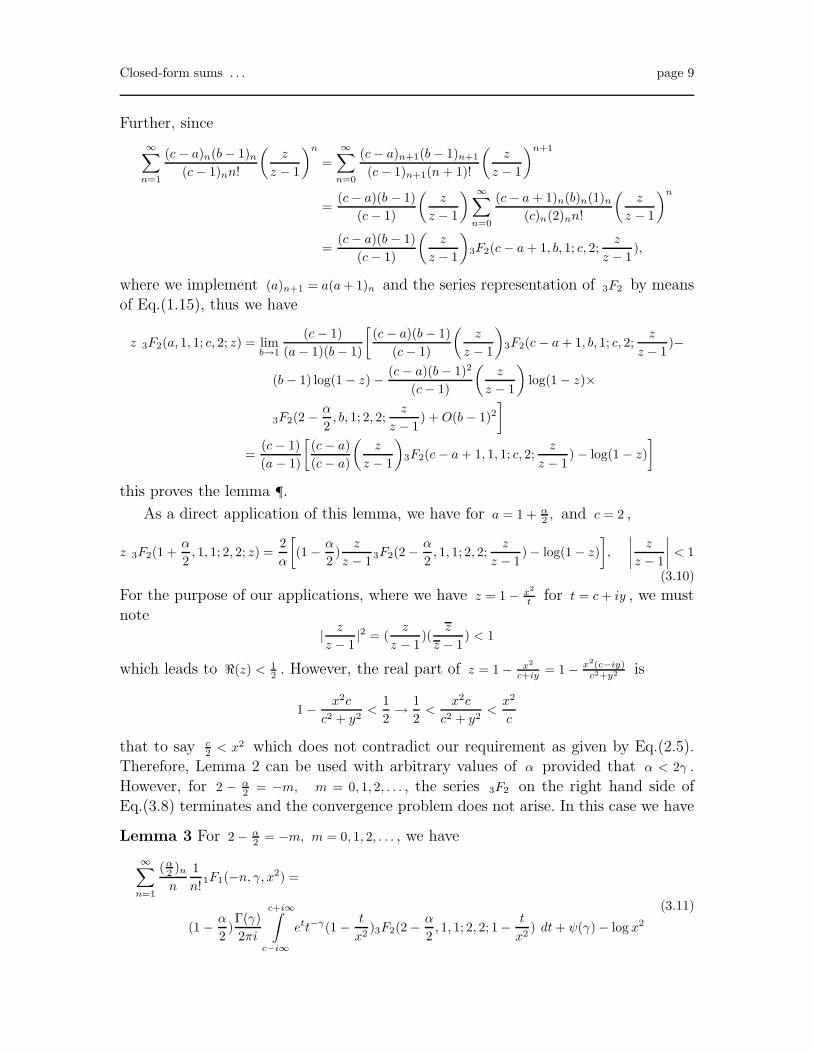
Closed-form sums . . . page 9

Further, since

∞∑

n=1

(c− a)n(b− 1)n

(c− 1)nn!

(

z

z − 1

)n

=

∞∑

n=0

(c− a)n+1(b− 1)n+1

(c− 1)n+1(n+ 1)!

(

z

z − 1

)n+1

=(c− a)(b − 1)

(c− 1)

(

z

z − 1

) ∞∑

n=0

(c− a+ 1)n(b)n(1)n

(c)n(2)nn!

(

z

z − 1

)n

=(c− a)(b − 1)

(c− 1)

(

z

z − 1

)

3F2(c− a+ 1, b, 1; c, 2;z

z − 1),

where we implement (a)n+1 = a(a+ 1)n and the series representation of 3F2 by means

of Eq.(1.15), thus we have

z 3F2(a, 1, 1; c, 2; z) = limb→1

(c− 1)

(a− 1)(b− 1)

[

(c− a)(b− 1)

(c− 1)

(

z

z − 1

)

3F2(c− a+ 1, b, 1; c, 2;z

z − 1)−

(b− 1) log(1 − z) − (c− a)(b− 1)2

(c− 1)

(

z

z − 1

)

log(1 − z)×

3F2(2 − α

2, b, 1; 2, 2;

z

z − 1) +O(b − 1)2

]

=(c− 1)

(a− 1)

[

(c− a)

(c− a)

(

z

z − 1

)

3F2(c− a+ 1, 1, 1; c, 2;z

z − 1) − log(1 − z)

]

this proves the lemma ¶.

As a direct application of this lemma, we have for a = 1 + α2 , and c = 2 ,

z 3F2(1 +α

2, 1, 1; 2, 2; z) =

2

α

[

(1 − α

2)

z

z − 13F2(2 − α

2, 1, 1; 2, 2;

z

z − 1) − log(1 − z)

]

,

∣

∣

∣

∣

z

z − 1

∣

∣

∣

∣

< 1

(3.10)

For the purpose of our applications, where we have z = 1 − x2

t for t = c+ iy , we must

note| z

z − 1|2 = (

z

z − 1)(

z

z − 1) < 1

which leads to ℜ(z) < 12 . However, the real part of z = 1 − x2

c+iy = 1 − x2(c−iy)c2+y2 is

1 − x2c

c2 + y2<

1

2→ 1

2<

x2c

c2 + y2<x2

c

that to say c2 < x2 which does not contradict our requirement as given by Eq.(2.5).

Therefore, Lemma 2 can be used with arbitrary values of α provided that α < 2γ .

However, for 2 − α2 = −m, m = 0, 1, 2, . . . , the series 3F2 on the right hand side of

Eq.(3.8) terminates and the convergence problem does not arise. In this case we have

Lemma 3 For 2 − α2 = −m, m = 0, 1, 2, . . . , we have

∞∑

n=1

(α2 )n

n

1

n!1F1(−n, γ, x2) =

(1 − α

2)Γ(γ)

2πi

c+i∞∫

c−i∞

ett−γ(1 − t

x2)3F2(2 − α

2, 1, 1; 2, 2; 1− t

x2) dt+ ψ(γ) − log x2

(3.11)

Closed-form sums . . . page 10

Proof: Using Lemma 2, and the fact that z = 1 − x2

t , Eq. (2.9) leads to

∞∑

n=1

(α2 )n

n

1

n!1F1(−n, γ, x2) =(1 − α

2)Γ(γ)

2πi

c+i∞∫

c−i∞

ett−γ(1 − t

x2)3F2(2 − α

2, 1, 1; 2, 2; 1− t

x2) dt

− Γ(γ)

2πi

c+i∞∫

c−i∞

ett−γ log(x2

t) dt

(3.12)

The second integral on the right hand side of Eq.(3.12) is already computed by meansof Lemma 1 and leads to

Γ(γ)

2πi

c+i∞∫

c−i∞

ett−γ log(x2

t) dt = log x2 − ψ(γ)

which completes the proof of the lemma ¶.

3.1. The case α = 4

In this case 2 − α2 = 0 , and Lemma 3 leads to

∞∑

n=1

(2)n

n n!1F1(−n, γ, x2) = −Γ(γ)

2πi

c+i∞∫

c−i∞

ett−γ(1 − t

x2) dt+ ψ(γ) − log x2

= −Γ(γ)

2πi

c+i∞∫

c−i∞

ett−γdt+1

x2

Γ(γ)

2πi

c+i∞∫

c−i∞

ett−γ+1dt

+ ψ(γ) − log x2

=γ − 1

x2− 1 + ψ(γ) − log x2, γ > 2,

(3.1.1)

where we invoke Eq.(3.2). There is, indeed, an independent confirmation for thisresult. Since (2)n = (1 + n)(1)n , the infinite sum in Eq.(1.13), reads

∞∑

n=1

1 + n

n1F1(−n; γ;x2) =

∞∑

n=1

1

n1F1(−n; γ;x2) +

∞∑

n=1

1F1(−n; γ;x2), (3.1.2)

The first series on the right hand side is summable by means of Toscano’s result [8]

(regardless the integral representation). For the second sum on the right hand side,we refer to Buchholz’s identity [11] ,

∞∑

n=0

(−ν)nΓ(γ + ν + 1)

Γ(n+ γ + 1)L(γ)

n (y) = yν , γ + ν > −1, ν 6= 0, 1, 2, . . . (3.1.3)

using Eq.(3.5), we have

∞∑

n=0

(−ν)nΓ(γ + ν + 1)

n!Γ(γ + 1)1F1(−n; γ + 1; y) = yν , γ + ν > −1 (3.1.4)

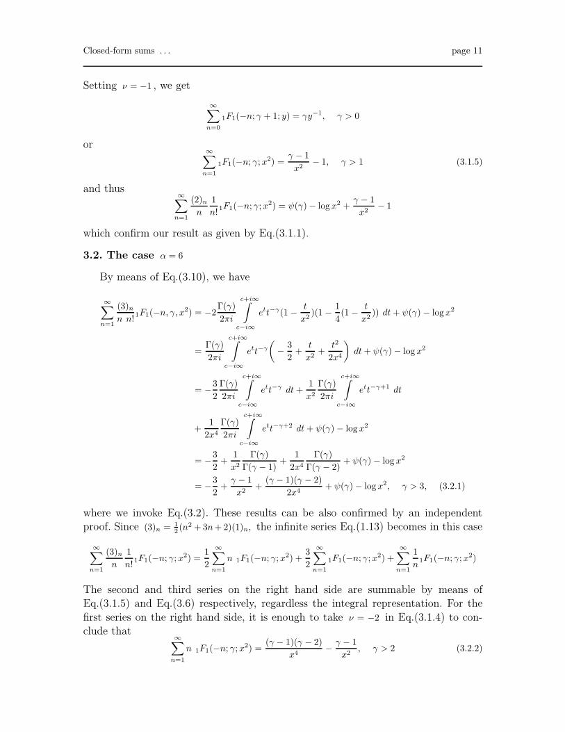
Closed-form sums . . . page 11

Setting ν = −1 , we get

∞∑

n=0

1F1(−n; γ + 1; y) = γy−1, γ > 0

or∞∑

n=1

1F1(−n; γ;x2) =γ − 1

x2− 1, γ > 1 (3.1.5)

and thus∞∑

n=1

(2)n

n

1

n!1F1(−n; γ;x2) = ψ(γ) − log x2 +

γ − 1

x2− 1

which confirm our result as given by Eq.(3.1.1).

3.2. The case α = 6

By means of Eq.(3.10), we have

∞∑

n=1

(3)n

n n!1F1(−n, γ, x2) = −2

Γ(γ)

2πi

c+i∞∫

c−i∞

ett−γ(1 − t

x2)(1 − 1

4(1 − t

x2)) dt+ ψ(γ) − log x2

=Γ(γ)

2πi

c+i∞∫

c−i∞

ett−γ

(

− 3

2+

t

x2+

t2

2x4

)

dt+ ψ(γ) − log x2

= −3

2

Γ(γ)

2πi

c+i∞∫

c−i∞

ett−γ dt+1

x2

Γ(γ)

2πi

c+i∞∫

c−i∞

ett−γ+1 dt

+1

2x4

Γ(γ)

2πi

c+i∞∫

c−i∞

ett−γ+2 dt+ ψ(γ) − log x2

= −3

2+

1

x2

Γ(γ)

Γ(γ − 1)+

1

2x4

Γ(γ)

Γ(γ − 2)+ ψ(γ) − log x2

= −3

2+γ − 1

x2+

(γ − 1)(γ − 2)

2x4+ ψ(γ) − log x2, γ > 3, (3.2.1)

where we invoke Eq.(3.2). These results can be also confirmed by an independentproof. Since (3)n = 1

2 (n2 + 3n+ 2)(1)n, the infinite series Eq.(1.13) becomes in this case

∞∑

n=1

(3)n

n

1

n!1F1(−n; γ;x2) =

1

2

∞∑

n=1

n 1F1(−n; γ;x2) +3

2

∞∑

n=1

1F1(−n; γ;x2) +∞∑

n=1

1

n1F1(−n; γ;x2)

The second and third series on the right hand side are summable by means ofEq.(3.1.5) and Eq.(3.6) respectively, regardless the integral representation. For the

first series on the right hand side, it is enough to take ν = −2 in Eq.(3.1.4) to con-clude that

∞∑

n=1

n 1F1(−n; γ;x2) =(γ − 1)(γ − 2)

x4− γ − 1

x2, γ > 2 (3.2.2)

Closed-form sums . . . page 12

This leads to

∞∑

n=1

(3)n

n

1

n!1F1(−n; γ;x2) =

γ − 1

x2− 3

2+

(γ − 1)(γ − 2)

2x4− log x2 + ψ(γ), γ > 3

IV. General Case

The results just mentioned for α = 4 and α = 6 can be generalized indeed to any

α such that 2 − α2 = −m,m = 0, 1, 2, . . . .

Lemma 4 For 2 − α2 = −m, m = 0, 1, 2, . . . and γ > α

2 , we have

∞∑

n=1

(α2 )n

n n!1F1(−n; γ;x2) =ψ(γ) − log x2 − (m+ 1)

m∑

k=0

(−m)k(1)k

(2)k(2)k

[

2F0(−k, 1 − γ;−;− 1

x2)

− γ − 1

x2 2F0(−k, 2 − γ;−;− 1

x2)

]

. (4.1)

Proof: Using Lemma 3, we have for 2 − α2 = −m, m = 0, 1, 2, . . . ,

∞∑

n=1

(α2 )n

n

1

n!1F1(−n, γ, x2) = ψ(γ)−log x2−(m+1)

Γ(γ)

2πi

c+i∞∫

c−i∞

ett−γ(1− t

x2)3F2(−m, 1, 1; 2, 2; 1− t

x2) dt

The function 3F2(−m, 1, 1; 2, 2; 1− tx2 ) is a terminated series, specifically a polynomial of

degree m , and therefore we may integrate term by term using the series representation

of 3F2. We have

Iγm(x) = −(m+ 1)

Γ(γ)

2πi

c+i∞∫

c−i∞

ett−γ(1 − t

x2)3F2(−m, 1, 1; 2, 2; 1− t

x2) dt

= −(m+ 1)Γ(γ)

2πi

m∑

k=0

(−m)k(1)k

(2)k(2)k

[

c+i∞∫

c−i∞

ett−γ(1 − t

x2)k dt− 1

x2

c+i∞∫

c−i∞

ett−γ+1(1 − t

x2)k dt

]

.

Since

(1 − t

x2)k =

k∑

l=0

(−k)l

l!(t

x2)l, finite number of terms,

we have

Iγm(x) = −(m+ 1)

m∑

k=0

(−m)k(1)k

(2)k(2)k

[ k∑

l=0

(−k)l

l!

1

x2l

Γ(γ)

2πi

c+i∞∫

c−i∞

ett−γ+l dt

−k

∑

l=0

(−k)l

l!

1

x2l+2

Γ(γ)

2πi

c+i∞∫

c−i∞

ett−γ+l+1 dt

]

= −(m+ 1)m

∑

k=0

(−m)k(1)k

(2)k(2)k

[ k∑

l=0

(−k)l

l!

1

x2l

Γ(γ)

Γ(γ − l)−

k∑

l=0

(−k)l

l!

1

x2l+2

Γ(γ)

Γ(γ − l − 1)

]

Closed-form sums . . . page 13

where we have used Eq.(3.2) for γ > l + 1 . From the identity Γ(γ − l) = Γ(γ)(γ)−l =

Γ(γ) (−1)l

(1−γ)land Γ(γ − l − 1) = Γ(γ − 1)(γ − 1)l = Γ(γ − 1) (−1)l

(2−γ)l, we have now

Iγm(x) = −(m+ 1)

m∑

k=0

(−m)k(1)k

(2)k(2)k

[ k∑

l=0

(−k)l(1 − γ)l

l!(− 1

x2)l − (γ − 1)

x2

k∑

l=0

(−k)l(2 − γ)l

l!(− 1

x2)l

]

which finally leads to

Iγm(x) = −(m+ 1)

m∑

k=0

(−m)k(1)k

(2)k(2)k

[

2F0(−k, 1 − γ;−;− 1

x2) − (γ − 1)

x2 2F0(−k, 2 − γ;−;− 1

x2)

]

by means of Eq.(1.15) ¶.

The significance of this lemma is that the infinite series of Eq.(2.9) can now bereplaced by a finite series that is much easier to calculate. To illustrate the use of this

lemma, we shall find now the infinite series of Eq.(2.9) for the case α = 8 , i.e. m = 2 ,since

∞∑

n=1

(4)n

n n!1F1(−n; γ;x2) =ψ(γ) − log x2 − 3

2∑

k=0

(−m)k(1)k

(2)k(2)k

[

2F0(−k, 1 − γ;−;− 1

x2)

− γ − 1

x2 2F0(−k, 2 − γ;−;− 1

x2)

]

and since

2F0(0, 1 − γ;−;− 1

x2) = 1

2F0(−1, 1 − γ;−;− 1

x2) = 1 − (γ − 1)

x2

2F0(−2, 1 − γ;−;− 1

x2) = 1 − 2(γ − 1)

x2+

(γ − 1)(γ − 2)

x4

and similarly for 2F0(−k, 2 − γ;−;− 1x2 ) , k = 0, 1, 2 . It is straightforward calculation to

find a closed-form sum for the infinite series Eq.(2.9) for α = 8 which leads in thiscase to

∞∑

n=1

(4)n

n n!1F1(−n; γ;x2) = ψ(γ) − log x2 − 11

6+

(γ − 1)(γ − 2)(γ − 3)

3x6+

(γ − 1)(γ − 2)

2x4+

(γ − 1)

x2,

(4.2)

valid for γ > 4 . It is interesting to mention here that the result of Lemma 4, can be

written in terms of the well-known associated Laguerre polynomials. Indeed, from theidentity [12]

(−1)nLa−nk (y) =

yn

n!2F0(−n,−a;−;−1

y),

the result of Lemma 4 can be written as

∞∑

n=1

(α2 )n

n n!1F1(−n; γ;x2) = ψ(γ) − log x2 − (m+ 1)

m∑

k=0

(−m)k

(k + 1)2

(

− 1

x2

)k[

Lγ−1−kk (x2)

− (γ − 1)

x2L

γ−2−kk (x2)

]

(4.3)

Closed-form sums . . . page 14

for α2 = 2 +m, m = 0, 1, 2, . . . .

V. Concluding Remarks

It is important to notice for x = 0 , the infinite series Eq.(1.13) for α ≥ 2 indeed

diverges. This follows from the fact that 1F1(−n; γ; 0) = 1 and

∞∑

n=1

(α2 )n

n

1

n!=α

2

∞∑

n=0

(1 + α2 )n(1)n

(2)n

(1)n

(2)n n!=α

23F2(1 +

α

2, 1, 1; 2, 2; 1)

which is absolutely convergent for α < 2 . Therefore, for our results concerning α =

2, 4, . . . and for the integral representation Eq.(2.9) in general, we must consider x > 0 .

The divergence of the infinite series in the expression of the first order perturbationcorrection of the wavefunction Eq.(1.12) as x → 0 is indeed controlled by the coeffi-

cient term xγ−1/2 as well by the coefficient e−x2

2 for x → ∞ . To illustrate the pointfurther, we consider the case of α = 2 , in this case the infinite series in Eq.(1.12) is

summable by means of Lemma 1 and the the first-order perturbation correction nowreads

ψ(1)0 (x) =

1√2

1

(γ − 1)√

Γ(γ)xγ− 1

2 e−x2

2 [log x− 1

2ψ(γ)] γ > 1. (5.1)

Since limx→0

xγ− 1

2 log x = 0 for γ > 1 , we have ψ(1)0 (0) = 0 . Consequently, the closed form

sums of the infinite series Eq.(1.13) contribute for intermediate values 0 < x < ∞ ofthe wave function rather than the boundaries.

The question posed by Aguillera-Navarro and Guardiola [1] concerning a special

summation formula for Eq.(1.2) in the case of α = 2 can now be answered with theaid of Lemma 1, which leads to

∞∑

n=1

1

n1F1(−n;

3

2;x2) = ψ(

3

2) − log x2, (5.2)

and the first order perturbation correction is given by means of Eq.(5.1) as

ψ(1)0 (x) = 2π−1/4xe−

x2

2 [log x− 1

2ψ(

3

2)] (5.3)

which matches the first-order perturbation correction expansion, in powers of λ , ofthe exact wave function ψ0(x) , that is Eq.(1.6).

The condition γ > α2 , α = 2, 4, 6 . . . , imposed on the closed form sums is too

strong, for they are indeed valid for weaker conditions. For example,

∞∑

n=1

1

n1F1(−n, γ, x2) = ψ(γ) − log x2, valid for all γ > 0,

∞∑

n=1

n+ 1

n1F1(−n, γ, x2) =

γ − 1

x2− 1 + ψ(γ) − log x2, valid for all γ > 1,

∞∑

n=1

12 (n2 + 3n+ 2)

n1F1(−n, γ, x2) = −3

2+γ − 1

x2+

(γ − 1)(γ − 2)

2x4+ψ(γ)−logx2, valid for all γ > 2.

Closed-form sums . . . page 15

However the condition has been imposed in order to meet the matrix elements’ con-vergence requirements.

Acknowledgment

Partial financial support of this work under Grant No. GP3438 from the NaturalSciences and Engineering Research Council of Canada is gratefully acknowledged by

one of us [RLH].

Closed-form sums . . . page 16

References

[1] V. C. Aguilera-Navarro and R. Guardiola, J. Math. Phys.32, 2135 (1991).

[2] R. Hall, N. Saad and A. von Keviczky, J. Phys. A: Math. Gen.34, 1169 (2001).

[3] R. Hall, N. Saad and A. von Keviczky, J. Math. Phys.39, 6345-51 (1998).

[4] R. Hall and N. Saad, J. Phys. A: Math. Gen.33, 569 (2000).

[5] R. Hall and N. Saad, J. Phys. A: Math. Gen.33, 5531 (2000).

[6] Yudell L. Luke, The Special Functions and their Approximation (Academic Press,

1969). Page 116, formula 3

[7] Yudell L. Luke, The Special Functions and their Approximation (Academic Press,1969). Page 17, formula 5

[8] Nota di Letterio Toscano, Boll. Un. Mat. Ital.3, 398 (1949).

[9] Yudell L. Luke, The Special Functions and their Approximation (Academic Press,

1969). Page 111, formula 40

[10] G. E. Andrews, R. Askey and R. Roy, Special Functions (Cambridge UniversityPress, 1999). Theorem 2.2.5, Page 68

[11] H. Buchholz, The Confluent Hypergeometric Function (Springer, 1969). Page 144,

last paragraph

[12] Elna B. McBride, Obtaining Generating Functions (Springer, 1971). Page 68, lastparagraph