www.elsevier.nl/locate/cam

Inner products involving q-di�erences:the little q-Laguerre–Sobolev polynomials

I. Areaa, E. Godoyb, F. Marcell�anc;∗, J.J. Moreno-Balc�azard;eaDepartamento de Matem�atica Aplicada, Escola Polit�ecnica Superior, Universidade de Santiago de Compostela,

Campus de Lugo, 27002 Lugo, SpainbDepartamento de Matem�atica Aplicada, E.T.S.I. Industriales y Minas, Universidad de Vigo,

Campus Lagoas-Marcosende, 36200 Vigo, SpaincDepartamento de Matem�aticas, Escuela Polit�ecnica Superior, Universidad Carlos III, C. Butarque, 15,

28911 Legan�es-Madrid, SpaindDepartamento de Estad ��stica y Matem�atica Aplicada, Edi�cio Cient ���co T�ecnico III, Universidad de Almer ��a,

04120 Almer ��a, SpaineInstituto Carlos I de F ��sica Te�orica y Computacional, Universidad de Granada, Spain

Received 13 January 1999

Abstract

In this paper, polynomials which are orthogonal with respect to the inner product

〈p; r〉S =∞∑k=0

p(qk)r(qk)(aq)k(aq; q)∞

(q; q)k+ �

∞∑k=0

(Dqp)(qk)(Dqr)(q

k)(aq)k(aq; q)∞

(q; q)k;

where Dq is the q-di�erence operator, �¿0; 0¡q¡ 1 and 0¡aq¡1 are studied. For these polynomials, algebraicproperties and q-di�erence equations are obtained as well as their relation with the monic little q-Laguerre polynomials.Some properties about the zeros of these polynomials are also deduced. Finally, the relative asymptotics {Qn(x)=pn(x; a|q)}non compact subsets of C \ [0; 1] is given, where Qn(x) is the nth degree monic orthogonal polynomial with respect to theabove inner product and pn(x; a|q) denotes the monic little q-Laguerre polynomial of degree n. c© 2000 Elsevier ScienceB.V. All rights reserved.

MSC: primary 33C25; secondary 33D45

Keywords: Orthogonal polynomials; Sobolev orthogonal polynomials; Little q-Laguerre polynomials

∗ Corresponding author.E-mail addresses: area@lugo.usc.es (I. Area), egodoy@dma.uvigo.es (E. Godoy), pacomarc@ing.uc3m.es

(F. Marcell�an), jmoreno@ualm.es (J.J. Moreno-Balc�azar)

0377-0427/00/$ - see front matter c© 2000 Elsevier Science B.V. All rights reserved.PII: S 0377-0427(00)00278-8

1

1. Introduction

The original motivation for considering Sobolev orthogonal polynomials comes from the least-squares approximation problems [15]. More precisely, for a given function the problem was to �ndits best polynomial approximant of degree n with respect to the norm

||g(x)||2 =∫R[g(x)]2 d�0(x) + �

∫R[g′(x)]2 d�1(x)

over all g ∈ C(1), being �i(x); i = 0; 1, positive Borel measures on the real line R having boundedor unbounded support [4,6,19].Also, in order to �nd the best polynomial approximation p(x) of a function f(x) where besides

function values f(xi) also di�erence derivatives at the knots are given, the following minimizationproblem appears in a natural way:

minr∑k=0

(bk−k−1∑xs=ak

(�kp(xs)− �kf(xs))2!k(xs));

�h(x) = h(x + 1)− h(x);�kh(x) = �k−1(�h(x));

where !k(x) are discrete weight functions on [ak ; bk), i.e., each !k(x) is the piecewise constantfunction with jumps !k(xi) at the points x = xi for which xi+1 = xi + 1 and ak6xi6bk − 1. In thissituation, it seems to be interesting the analysis of the polynomials which are orthogonal with respectto the inner product

(p; q)S =r∑k=0

(bk−k−1∑xs=ak

�kp(xs)�kq(xs)!k(xs)

):

In recent works [1,2], we have studied algebraic and analytic properties of the polynomialsorthogonal with respect to a particular case (r = 1; !0 ≡ !1) of the above inner product

〈p; q〉=∞∑s=0

p(s)q(s)!(s) + �∞∑s=0

�p(s)�q(s)!(s);

where �¿0 and !(s) is the Pascal distribution from probability theory, !(s)=�s�(�+s)=�(s+1)�(�),�¿ 0, 0¡�¡ 1. For �=0 the corresponding polynomials are the Meixner polynomials, introducedin [23].Moreover, if the knots are xi+1 = qxi (nonequidistant mesh widths), where q is a real number

q �= 1, and if we want to involve in the approximation the value of the function at the knots as wellas the q-di�erences of the function, we arrive to the following minimization problem:

minr∑k=0

⎛⎝bk−qk−1∑

xs=ak

((Dkqp)(xs)− (Dkqf)(xs))2�k(xs)⎞⎠ with (Dkqh)(x) = (D

k−1q (Dqh))(x);

where �k are q-weight functions and the q-di�erence operator Dq is de�ned by

(Dqh)(x) =h(qx)− h(x)(q− 1)x ; x �= 0; q �= 1; (Dqh)(0) = h′(0):

2

Thus, the Fourier projector in terms of polynomials which are orthogonal with respect to the innerproduct

〈p; r〉W =r∑k=0

⎛⎝bk−qk−1∑

xs=ak

(Dkqp)(xs)(Dkqr)(xs)�k(xs)

⎞⎠

allows to give the explicit expression for such a best polynomial approximation. Since we aredealing with a nonuniform lattice [27], this q-approximation constitutes a natural tool for obtaininga more accurate estimation when the �rst derivative of the function to be approximated increasesvery quickly in a neighborhood of an end point.The aim of this paper is the study of polynomials which are orthogonal with respect to a particular

case (r = 1; �0 ≡ �1) of the above inner product

〈p; r〉S = 〈p; r〉+ �〈Dqp;Dqr〉=∞∑k=0

p(qk)r(qk)�(qk) + �∞∑s=0

(Dqp)(qk)(Dqr)(qk)�(qk); (1.1)

where �¿ 0 and� is the little q-Laguerre step function [3,5,13] whose jumps are �(qk)=(aq)k(aq; q)∞=(q; q)k , k=0; 1; 2; : : : ; 0¡aq¡ 1; 0¡q¡ 1. We call (1.1) the little q-Laguerre–Sobolev inner prod-uct, by analogy with the continuous case [20].Koekoek [11,12] studied the q-analogues of Sobolev-type orthogonal polynomials in the Laguerre

case. He de�ned the inner product on P, the linear space of polynomials with real coe�cients,

(f; g)S =�q(−)

�(−)�(+ 1)∫ ∞

0

x

(−(1− q)x; q)∞f(x)g(x) dx +N∑=0

M(Dqf)(0)(Dqg)(0);

where ¿ − 1, N is a nonnegative integer, M¿0 for all ∈{0; 1; 2; : : : ; N}. Note that the masspoints are zeros of the polynomial �(x) appearing in the Pearson-type q-di�erence equation for theorthogonality weight function �(x), i.e., (Dq(��))(x) = �(x)�(x). This location of the mass pointsallowed to the author to obtain a representation of the polynomials orthogonal with respect to theabove inner product as a basic hypergeometric series N+2’N+2. In the present work, we considera di�erent problem since we deal with an inner product involving q-di�erences of order 1 andnonatomic measures. Furthermore, if we consider an appropriate limit of the polynomials which areorthogonal with respect to (1.1) we recover the so-called Laguerre–Sobolev orthogonal polynomials(see e.g. [20,28]).The structure of the paper is as follows: Section 2 contains some basic de�nitions and notations as

well as the relations for monic little q-Laguerre polynomials {pn(x; a|q)}n which will be useful withinthe paper. In Section 3, we introduce the monic little q-Laguerre–Sobolev orthogonal polynomials{Qn(x)}n. In Section 4, a linear q-di�erence operator S on P is de�ned. We prove that S isa symmetric operator with respect to the little q-Laguerre–Sobolev inner product and we �nd anonstandard four-term recurrence relation for the polynomials {Qn(x)}n. In Section 5, we studythe zero distribution of little q-Laguerre–Sobolev orthogonal polynomials. Finally, in Section 6, therelative asymptotics {Qn(x)=pn(x; a|q)}n and the asymptotic behavior of the ratio of two consecutivelittle q-Laguerre–Sobolev orthogonal polynomials are obtained.

3

2. Basic de�nitions and notations

2.1. Linear functionals

Let P be the linear space of real polynomials and let P′ be its algebraic dual space. We denoteby (u; f) the duality bracket for u∈P′ and f∈P, and by (u)n = (u; xn), with n¿0, the canonicalmoments of u.

De�nition 1. Given a real number c, the Dirac functional �c is de�ned by (�c; p(x)):=p(c), forevery p∈P.

De�nition 2. Given a linear functional u, we de�ne, for each polynomial p, the linear functional puas follows (pu; r(x)):=(u; p(x)r(x)), for every r ∈P. For each real number c the linear functional(x − c)−1u is given by

((x − c)−1u; r(x)):=(u; (r(x)− r(c))=(x − c)) for every r ∈P: (2.1)

Note that

(x − c)−1((x − c)u) = u − (u)0�c for every u∈P′; (2.2)

while

(x − c)((x − c)−1u) = u: (2.3)

2.2. Monic little q-Laguerre orthogonal polynomials

In what follows, we shall always assume that 0¡q¡ 1. The q-derivative operator Dq is de�nedby [7, Eq. (2.3)]

(Dqp)(x) =p(qx)− p(x)(q− 1)x ; x �= 0 (2.4)

and (Dqp)(0) = p′(0) by continuity, for p∈P. Note that limq↑1 (Dqp)(x) = p′(x), for every p∈P.This q-di�erence operator satis�es the following properties which will be useful in the next sections:

(Dq(pr))(x) = r(x)(Dqp)(x) + p(qx)(Dqr)(x) for every r; p∈P: (2.5)

(Dqp)(x) = (Dq−1p)(qx) for every p∈P: (2.6)

Monic little q-Laguerre polynomials pn(x; a|q) are the polynomials orthogonal with respect to theinner product (see [13])

〈p; r〉=∞∑k=0

(aq)k(aq; q)∞(q; q)k

p(qk)r(qk); 0¡aq¡ 1; for every p; r ∈P; (2.7)

4

where the q-shifted factorials are de�ned [5, pp. 3,6]

(b; q)0 = 1; (b; q)k =k∏j=1

(1− bqj−1); k¿1 and (b; q)∞ = limn→∞(b; q)n =

∞∏j=1

(1− bqj−1):(2.8)

Using the q-integral introduced by Thomae [30,31] and Jackson [10]∫ b

0f(x)dq(x):=(1− q)b

∞∑n=0

f(bqn)qn; b¿ 0

and since (q; q)k = (q; q)∞=(qk+1; q)∞, the inner product (2.7) can be written for a= q as

〈p; r〉= (q+1; q)∞(1− q)(q; q)∞

∫ 1

0p(x)r(x)x(qx; q)∞dq(x); ¿ − 1:

Little q-Laguerre polynomials are a particular family of little q-Jacobi polynomials and they con-stitute q-analogues of Laguerre polynomials (see [14, p. 117] and [8, p. 272]). They are related withmonic orthogonal Wall polynomials {Wn(x; b; q)}n (see [3,5, p. 198, p. 196]) as follows:

pn(x; a|q) = Wn(qx; aq; q)qn

; n¿0:

They are also related with monic q-Laguerre polynomials {L()n (x; q)}n (see [5,9,25, p. 194]) by

pn(x; q|q) =(1− qq

)nL()n

(qx1− q ; q

); n¿0; ¿ − 1:

For monic little q-Laguerre polynomials the following properties are known.

2.2.1. Three-term recurrence relationWe have [13]

xpn(x; a|q) = pn+1(x; a|q) + Bnpn(x; a|q) + Cnpn−1(x; a|q); n¿1;

Bn = qn(1 + a− aqn(q+ 1)); Cn = aq2n−1(qn − 1)(aqn − 1) (2.9)

with the initial conditions p0(x; a|q) = 1 and p1(x; a|q) = x − (1− aq).

2.2.2. q-di�erence representationsIn [22] we can �nd

pn(x; a|q) = Dqpn+1(x; a|q)[n+ 1]q+ aqn(1− q)Dqpn(x; a|q); n¿0; (2.10)

where

[0]q = 0; [n]q =qn − 1q− 1 ; n¿1: (2.11)

Moreover, since

pn(x; aq|q) = Dqpn+1(x; a|q)[n+ 1]q; n¿0;

5

we get

pn

(x;aq

∣∣∣∣ q)= pn(x; a|q) + aqn−1(1− qn)pn−1(x; a|q); n¿1: (2.12)

2.2.3. Representation as a basic hypergeometric functionWe have [5,14,22]

pn(x; a|q) = (−1)nqn(n−1)=2(aq; q)n 2’1(q−n; 0

aq

∣∣∣∣∣ q; qx)

= (−1)nqn(n−1)=2(aq; q)nn∑k=0

(q−n; q)k(q; q)k(aq; q)k

(qx)k : (2.13)

From the above hypergeometric representation we get

pn(0; a|q) = (−1)nqn(n−1)=2(aq; q)n: (2.14)

2.2.4. Squared norm and momentsLet us denote for n¿0,

kn = 〈pn(x; a|q); pn(x; a|q)〉=∞∑k=1

(aq)k(aq; q)∞(q; q)k

(pn(qk ; a|q))2 = (aqn)n(q; q)n(aq; q)n (2.15)

(see [13]). From the de�nition of kn we can deduce the following relations:

k0 = 1; kn = aq2 n−1(qn − 1)(aqn − 1)kn−1; n¿1: (2.16)

If we denote the little q-Laguerre linear functional u(a) as

(u(a); p(x)) =∞∑k=0

(aq)k(aq; q)∞(q; q)k

p(qk) for every p∈P (2.17)

then the canonical moments associated with u(a) can be derived from [3, p. 198] and they are

(u(a); xn) = (aq; q)n; n¿0: (2.18)

3. Little q-Laguerre–Sobolev orthogonal polynomials

Let us consider the Sobolev inner product de�ned on P by

〈p; r〉S =∞∑k=0

p(qk)r(qk)(aq)k(aq; q)∞

(q; q)k+ �

∞∑k=0

(Dqp)(qk)(Dqr)(qk)(aq)k(aq; q)∞

(q; q)k; (3.1)

where Dq is the q-di�erence operator de�ned in (2.4), 0¡aq¡ 1 and �¿0.We shall denote by {Qn(x; a; �|q)}n ≡ {Qn(x)}n the MOPS associated with the (Sobolev) inner

product 〈:; :〉S . Such a sequence is said to be the little q-Laguerre–Sobolev MOPS.

6

Proposition 1. Let {pn(x; a|q)}n be the little q-Laguerre MOPS and let {Qn(x)}n be the littleq-Laguerre–Sobolev MOPS. The following relation holds:

pn(x; a|q) + aqn−1(1− qn)pn−1(x; a|q) = Qn(x) + dn−1(�; a|q)Qn−1(x); n¿2; (3.2)

where

dn−1(�; a|q) ≡ dn−1(�) = aqn−1(1− qn) kn−1kn−1

; (3.3)

kn = 〈Qn; Qn〉S : (3.4)

Proof. If we expand

pn(x; a|q) + aqn−1(1− qn)pn−1(x; a|q) = Qn(x) +n−1∑i=0

fi;nQi(x);

then

fi;n =〈pn(x; a|q) + aqn−1(1− qn)pn−1(x; a|q); Qi(x)〉S

〈Qi; Qi〉S :

Thus, for 06i6n− 1 we have, by using (2.10),

fi;n=1

k i{〈pn(x; a|q) + aqn−1(1− qn)pn−1(x; a|q); Qi(x)〉S}

=1

k i{〈pn(x; a|q) + aqn−1(1− qn)pn−1(x; a|q); Qi(x)〉+ �[n]q〈pn−1(x; a|q); DqQi(x)〉}

=〈pn(x; a|q) + aqn−1(1− qn)pn−1(x; a|q); Qi(x)〉

k i:

Then,

fi;n =

⎧⎨⎩0 if 06i6n− 2;aqn−1(1− qn) kn−1

kn−1if i = n− 1:

Corollary 1. The little q-Laguerre–Sobolev orthogonal polynomials satisfy

Qn(x) =n∑j=1

ej;npj(x; a|q); n¿1; (3.5)

where

en;n = 1; (3.6)

ej;n = (−1)n−j(dj(�) + aqj(qj+1 − 1))n−1∏s=j+1

ds(�); 16j6n− 1; n¿2; (3.7)

with the convention∏m−1s=m ds(�) = 1.

7

Proof. From (3.2) and taking into account that Q1(x) = p1(x; a|q), (3.5) is derived.

We can compute recursively the coe�cients dn(�) and the norms kn de�ned in (3.3) and (3.4),respectively, by means of

Proposition 2. For n¿2; we have

dn(�) =−a2q3n+1(qn − 1)(aqn − 1)(qn+1 − 1)

aq2n+1(qn − 1)(aqn − 1) + ([n]q)2(�q2 + a2(q− 1)2q2n) + aqn+1(qn − 1)dn−1(�); (3.8)

with the initial condition

d1(�) =−a2(q− 1)q2(aq− 1)(q2 − 1)�+ a(q− 1)q(aq− 1) : (3.9)

Moreover; we have

kn = kn + (�+ (a(1− q)qn−1)2)([n]q)2kn−1 − (a(1− qn)qn−1)2(kn−1)2

kn−1; n¿1 (3.10)

with k0 = k0 = 1.

Proof. If we denote pn(x; a|q) ≡ pn(x), from the de�nition of kn in (3.4), using (2.10) and (3.2),we get

kn= 〈Qn(x); Qn(x)〉S = 〈Qn(x); pn(x)〉S = kn + �〈(DqQn)(x); (Dqpn)(x)〉= kn + �〈(DqQn)(x); [n]qpn−1(x)− a(1− q)[n]qqn−1(Dqpn−1)(x)〉= kn + �([n]q)

2kn−1 − �aqn−1(1− qn)〈(DqQn)(x); (Dqpn−1)(x)〉= kn + �([n]q)

2kn−1 − aqn−1(1− qn){〈Qn(x); pn−1(x)〉S − 〈Qn(x); pn−1(x)〉}= kn + �([n]q)

2kn−1 + aqn−1(1− qn)〈Qn(x); pn−1(x)〉= kn + �([n]q)

2kn−1 + aqn−1(1− qn)×〈pn(x) + aqn−1(1− qn)pn−1(x)− dn−1(�)Qn−1(x); pn−1(x)〉

= kn + �([n]q)2kn−1 + (aqn−1(1− qn))2kn−1 − aqn−1(1− qn)dn−1(�)kn−1:

Thus, from (2.16) and (3.3) we get (3.8) as well as the initial condition (3.9). Eq. (3.10) is aconsequence of the above equality and (3.3).

Remark. Although the coe�cients dn(�) appear in the previous results for n¿1, we can start therecurrence relation (3.8) with the initial condition d0(�) = a(1− q), obtaining the same coe�cientsfor n¿1.

Monic little q-Laguerre orthogonal polynomials {pn(x; a|q)}n are related with monic Laguerreorthogonal polynomials {L()n (x)}n by means of the following limit relation (see [13, p. 105])

limq↑1

pn((1− q)x; q|q)(1− q)n = L()n (x); n¿0; ¿−1: (3.11)

8

Monic Laguerre–Sobolev polynomials {Q()n (x)}n (see e.g. [20,28]) are the polynomials orthogonalwith respect to the Sobolev inner product

(p; r)S =∫ ∞

0p(x)r(x)xe−x + �

∫ ∞

0p(x)r(x)xe−x; ¿−1: (3.12)

Monic Laguerre–Sobolev polynomials and monic Laguerre polynomials are related by means of

Q()n (x) + dn−1(�; )Q()n−1(x) = L

()n (x) + nL

()n−1(x); (3.13)

where the coe�cients dn(�; ) satisfy the following �rst-order recurrence relation

dn(�; ) =(1 + n)(+ n)

+ (2 + �)n− dn−1(�; ) ; d1(�; ) =2(1 + )1 + + �

: (3.14)

A limit relation between monic little q-Laguerre–Sobolev orthogonal polynomials and monicLaguerre–Sobolev orthogonal polynomials appears in a natural way.

Proposition 3. The following limit relation holds:

limq↑1

Qn((1− q)x; q; �(1− q)2|q)(1− q)n = Q()n (x); n¿1; (3.15)

where {Q()n (x)}n are the monic Laguerre–Sobolev polynomials.

Proof. From (3.2) we have for n¿2,Qn((1− q)x; q; �(1− q)2|q)

(1− q)n =pn((1− q)x; q|q)

(1− q)n + q[n]qqn−1pn−1((1− q)x; q|q)

(1− q)n−1

− dn−1(�(1− q)2; q|q)

(1− q)Qn−1((1− q)x; q; �(1− q)2|q)

(1− q)n−1 : (3.16)

Since limq↑1 [n]q = n and dn(�(1 − q)2; q|q)=(1 − q) converges to the coe�cients dn(�; ) given in(3.14) when q ↑ 1, the result follows by using the limit relation (3.11) as well as the equality

Q1((1− q)x; q; �(1− q)2|q) = p1((1− q)x; q|q):

4. The linear operator S

Even the inner product in (3.1) no longer satis�es the basic property 〈xp(x); r(x)〉S=〈p(x); xr(x)〉S ;i.e. {Qn}n does not satisfy a three-term recurrence relation, there exists an operator S which issymmetric with respect to the inner product (3.1).

Proposition 4. Let h(x) be the polynomial

h(x) = a(q− 1)x (4.1)

with 0¡aq¡ 1; and let S be the q-di�erence operator

S ≡ h(x)I − �aDq + �(1− x)Dq−1 ; (4.2)

where I is the identity operator. Then

〈h(x)p(x); r(x)〉S = 〈p(x); (Sr)(x)〉 for every p; r ∈P: (4.3)

9

Proof. The weight function

�(qk) =(aq)k(aq; q)∞

(q; q)ksatis�es

(1− qk)�(qk) = aq�(qk−1); k¿1: (4.4)

Using (2.5) we get

〈h(x)p(x); r(x)〉S = 〈h(x)p(x); r(x)〉+ �〈(Dq(hp))(x); (Dqr)(x)〉= 〈h(x)p(x); r(x)〉 − �a〈p(x); (Dqr)(x)〉+ �aq〈p(qx); (Dqr)(x)〉= 〈p(x); h(x)r(x)− �a(Dqr)(x)〉+ �〈(1− x)p(x); (Dq−1r)(x)〉;

where the last equality is a consequence of (4.4). Then, the result holds.

Theorem 1. The linear operator S de�ned in (4:2) is symmetric with respect to the Sobolev innerproduct (3:1); i.e.;

〈(Sp)(x); r(x)〉S = 〈p(x); (Sr)(x)〉S for every p; r ∈P: (4.5)

Proof. Since S is a linear operator, it is su�cient to prove that

〈(S#n)(x); #m(x)〉S − 〈#n(x); (S#m)(x)〉S = 0 for every n; m¿0; (4.6)

with #k(x) = xk .If n+ m62, it is easy to obtain the result for each particular case.On the other hand, if n+m¿ 2, from (2.17) and (4.2) the left-hand side of (4.6) is (u(a); tn+m(x)),

where

tn+m(x) = �q{(q−m[m]q − q−n[n]q)xn+m + ((a− q−m)[m]q − (a− q−n)[n]q)xn+m−1}+ �2q1−m−n[n]q[m]q{(qn[m]q − qm[n]q)xn+m−2

+ (qm(1− aqn−1)[n− 1]q − qn(1− aqm−1)[m− 1]q)xn+m−3}: (4.7)

From (2.18) and after some straightforward computations we deduce that (u(a); tn+m(x)) = 0:

Proposition 5. Let {pn(x; a|q)}n be the little q-Laguerre MOPS and {Qn(x)}n be the littleq-Laguerre–Sobolev MOPS. We have

h(x)pn(x; a|q) = a(q− 1)Qn+1(x) + an;nQn(x) + an−1; nQn−1(x); n¿2; (4.8)

where

an;n = a(q− 1)(dn(�) + qn(1− aqn)); (4.9)

an−1; n = aqn(q− 1)(1− aqn)dn−1(�) (4.10)

with h(x) and dn(�) de�ned in (4:1) and (3:3); respectively.

10

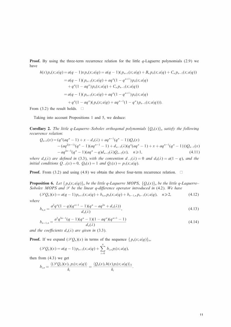
Proof. By using the three-term recurrence relation for the little q-Laguerre polynomials (2.9) wehave

h(x)pn(x; a|q) = a(q− 1)xpn(x; a|q) = a(q− 1)(pn+1(x; a|q) + Bnpn(x; a|q) + Cnpn−1(x; a|q))= a(q− 1)(pn+1(x; a|q) + aqn(1− qn+1)pn(x; a|q)+ qn(1− aqn)pn(x; a|q) + Cnpn−1(x; a|q))

= a(q− 1)(pn+1(x; a|q) + aqn(1− qn+1)pn(x; a|q)+ qn(1− aqn)(pn(x; a|q) + aqn−1(1− qn)pn−1(x; a|q))):

From (3.2) the result holds.

Taking into account Propositions 1 and 5, we deduce:

Corollary 2. The little q-Laguerre–Sobolev orthogonal polynomials {Qn(x)}n satisfy the followingrecurrence relation:

Qn+1(x) = (qn(aqn − 1) + x − dn(�) + aqn−1(qn − 1))Qn(x)− (aq2(n−1)(qn − 1)(aqn−1 − 1) + dn−1(�)(qn(aqn − 1) + x + aqn−1(qn − 1)))Qn−1(x)− aq2n−3(qn − 1)(aqn − q)dn−2(�)Qn−2(x); n¿1; (4.11)

where dn(�) are de�ned in (3:3); with the convention d−1(�) = 0 and d0(�) = a(1 − q); and theinitial conditions Q−1(x) = 0; Q0(x) = 1 and Q1(x) = p1(x; a|q).

Proof. From (3.2) and using (4.8) we obtain the above four-term recurrence relation.

Proposition 6. Let {pn(x; a|q)}n be the little q-Laguerre MOPS; {Qn(x)}n be the little q-Laguerre–Sobolev MOPS and S be the linear q-di�erence operator introduced in (4:2). We have

(SQn)(x) = a(q− 1)pn+1(x; a|q) + bn;npn(x; a|q) + bn−1; npn−1(x; a|q); n¿2; (4.12)

where

bn;n =a2qn(1− q)(qn+1 − 1)(qn − aq2n + dn(�))

dn(�); (4.13)

bn−1; n =a3q3n−1(q− 1)(qn − 1)(1− aqn)(qn+1 − 1)

dn(�)(4.14)

and the coe�cients dn(�) are given in (3:3).

Proof. If we expand (SQn)(x) in terms of the sequence {pn(x; a|q)}n,

(SQn)(x) = a(q− 1)pn+1(x; a|q) +n∑i=0

bi;npi(x; a|q);

then from (4.3) we get

bi;n =〈(SQn)(x); pi(x; a|q)〉

ki=

〈Qn(x); h(x)pi(x; a|q)〉Ski

:

11

Hence bi;n = 0 for i = 0; 1; : : : ; n− 2. On the other hand,

bn−1; n =〈Qn(x); h(x)pn−1(x; a|q)〉S

kn−1= a(q− 1) kn

kn−1and

bn;n=〈Qn(x); h(x)pn(x; a|q)〉S

kn

=〈Qn(x); a(q− 1)Qn+1(x) + an;nQn(x) + an−1; nQn−1(x)〉S

kn= an;n

knkn

using (4.8).

Proposition 7. Let {pn(x; a|q)}n be the little q-Laguerre MOPS; {Qn(x)}n be the little q-Laguerre–Sobolev MOPS and S be the linear q-di�erence operator de�ned in (4:2). The following relationholds:

(SQn)(x) = a(q− 1)Qn+1(x) + cn;nQn(x) + cn−1; nQn−1(x); n¿2; (4.15)

where

cn;n =a(q− 1)(aq2n(aqn − 1)(qn+1 − 1) + dn(�)2)

dn(�); (4.16)

cn−1; n =a2q2n(q− 1)(aqn − 1)(qn+1 − 1)dn−1(�)

dn(�)(4.17)

and the coe�cients dn(�) are given in (3:3).

Proof. If we expand the polynomial (SQn)(x) in terms of the polynomials {Qn(x)}n,

(SQn)(x) = a(q− 1)Qn+1(x) +n∑i=0

ci;nQi(x)

and using the symmetric character of the linear operator S, we get

ci;n =〈(SQn)(x); Qi(x)〉S〈Qi(x); Qi(x)〉S =

〈Qn(x); (SQi)(x)〉Sk i

:

Thus, ci;n = 0 for i = 0; 1; : : : ; n− 2. Moreover,

cn−1; n =〈Qn(x); (SQn−1)(x)〉S

kn−1= a(q− 1) kn

kn−1:

Finally, from Proposition 6 we get

cn;n=〈Qn(x); (SQn)(x)〉S

kn

=〈a(q− 1)pn+1(x; a|q) + bn;npn(x; a|q) + bn−1; npn−1(x; a|q); Qn(x)〉S

kn

= a(q− 1)〈pn+1(x; a|q); Qn(x)〉Skn

+ bn;n;

12

where bn;n is given in (4.13). So we must compute 〈pn+1(x; a|q); Qn(x)〉S . Since

bn;n =〈Qn(x); h(x)pn(x; a|q)〉S

kn= a(q− 1)〈Qn(x); xpn(x; a|q)〉S

kn

=a(q− 1)kn

(〈Qn(x); pn+1(x; a|q)〉S + Bnkn);where h(x) = a(q− 1)x and Bn is given in (2.9), we can express 〈pn+1(x; a|q); Qn(x)〉S in terms ofbn;n and after some straightforward computations the result holds.

5. Zeros

The zeros of the polynomial pn(x; a|q) are all real and distinct, they live on the interval oforthogonality (0; 1), and they separate the zeros of pn−1(x; a|q). In this section we study the locationof the zeros of little q-Laguerre–Sobolev orthogonal polynomials {Qn(x)}n. An interlacing propertywhich relates the zeros of Qn(x) with the zeros of pn(x; a|q) is proved.

Lemma 1. For n¿0 and a61 we have (−1)nQn(0)¿ 0.

Proof. We shall prove that Qn(0)=pn(0; a|q)¿ 0, for every n¿0. Thus, by using the value ofpn(0; a|q) given in (2.14) the result follows.From (3.2) we obtain the following recurrence relation for Qn(0):

Qn(0) = pn(0; a|q) + aqn−1(1− qn)pn−1(0; a|q)− dn−1(�)Qn−1(0);Q1(0) = p1(0; a|q):

By using (2.14),

pn(0; a|q) + aqn−1(1− qn)pn−1(0; a|q) = pn−1(0; a|q)qn−1(a− 1):Thus,

Qn(0) = pn−1(0; a|q)qn−1(a− 1)− dn−1(�)Qn−1(0); Q1(0) = p1(0; a|q) = aq− 1:From (2.14) we can also obtain

pn(0; a|q) = qn−1(aqn − 1)pn−1(0; a|q):Taking into account the last expression,

Qn(0)pn(0; a|q) =

a− 1aqn − 1 − dn−1(�)

qn−1(aqn − 1)Qn−1(0)

pn−1(0; a|q) :

If we denote An = Qn(0)=pn(0; a|q), the last equality readsAn =

a− 1aqn − 1 − dn−1(�)

qn−1(aqn − 1)An−1:

From (3.3) we obtain

A1 =Q1(0)

p1(0; a|q) = 1; An =1

1− aqn(1− a+ a(1− qn) kn−1

kn−1An−1

):

13

Since k1=k1¿ 0, the coe�cient A2 is positive for a61 and then An¿0, for every n¿1. Thus,sgn(Qn(0)) = sgn(pn(0; a|q)), for every n¿1, so we get Q2k(0)¿ 0 and Q2k+1(0)¡ 0. The casen= 0 follows from Q0(0) = p0(0; a|q) = 1.

Lemma 2. Let pk(x) be a polynomial of degree k. If �=0 or a=1; there exists a unique polynomialgk(x) of degree k such that

(Sgk)(x) = h(x)pk(x); (5.1)

where the linear operator S and the polynomial h(x) are de�ned in Proposition 4.

Proof. If � = 0 the linear operator S becomes h(x)I; where I stands for the identity operator.Then, it is su�cient to take gk(x) = pk(x).If a= 1 the linear operator S can be written

S ≡ (q− 1)xI − �Dq + �(1− x)Dq−1 :

Let us expand

gk(x) =k∑i=0

bixi; h(x)pk(x) = (q− 1)xpk(x) =k+1∑i=1

aixi:

The action of the linear operator S on gk(x) yields

(Sgk)(x) =k∑i=0

bi

((q− 1)xi+1 − � [i]q

qi−1xi + �[i]q

(1qi−1

− 1)xi−1

):

From the equality (Sgk)(x) = h(x)pk(x) we obtain a system of k + 1 linear equations withk + 1 unknowns. It has a unique solution which can be found by using the forward substitutionmethod.

Lemma 3. Let pk(x) be a polynomial of degree k and assume a=1. Let gk(x) be the polynomialof degree k given in Lemma 2 such that (Sgk)(x) = h(x)pk(x). Then

〈r(x); gk(x)〉S = 〈r(x); pk(x)〉 − �1− q r(0)(Dq−1gk)(0) for every r ∈P: (5.2)

Proof. For each polynomial r(x) we have

r(x) = r(qx)− h(x)(Dqr)(x): (5.3)

Since (Sgk)(0) = 0, from (2.1), (2.3), (2.6), (3.1), (4.2), (5.1) and (5.3) we get

〈r(x); pk(x)〉=⟨r(x);

(Sgk)(x)h(x)

⟩=

(u(1);

r(x)(Sgk)(x)h(x)

)

=(u(1);

r(x)(Sgk)(x)− r(0)(Sgk)(0)h(x)

)= ((h(x))−1u(1); r(x)(Sgk)(x))

= 〈r(x); gk(x)〉S − �((h(x))−1u(1); r(qx)(Dq−1gk)(qx)− r(x)(Dq−1gk)(x))

− �q− 1(u

(1); r(x)(Dq−1gk)(x))

14

= 〈r(x); gk(x)〉S − �((h(x))−1u(1); h(x)Dq[r(x)(Dq−1gk)(x)])

− �q− 1(u

(1); r(x)(Dq−1gk)(x))

= 〈r(x); gk(x)〉S − �(u(1); Dq[r(x)(Dq−1gk)(x)])− �q− 1(u

(1); r(x)(Dq−1gk)(x)):

Consequently, if we denote t(x) = r(x) (Dq−1gk)(x) we have

〈r(x); pk(x)〉= 〈r(x); gk(x)〉S − �(u(1); (Dqt)(x) +

t(x)q− 1

): (5.4)

Since t(x) is a polynomial, writing

t(x) =m∑k=0

tkxk ; (5.5)

we obtain(u(1); (Dqt)(x) +

t(x)q− 1

)=(u(1))0t0q− 1 +

m∑k=1

([k]q(u

(1))k−1 +(u(1))kq− 1

)tk (5.6)

and from (2.11) and (2.18) we get(u(1); (Dqt)(x) +

t(x)q− 1

)=

1q− 1 r(0)(Dq−1gk)(0): (5.7)

Substitution of this relation into (5.4) yields (5.2).

Lemma 4. Let pk(x) be a polynomial of degree k ¿ 1. If �¿ 0 and a �= 1; there exist a uniquepolynomial gk(x) of degree k and a unique constant cp (depending on the polynomial pk) such that

(Sgk)(x) = h(x)(pk(x) + xcp): (5.8)

Proof. Let us expand

gk(x) =k∑i=0

bixi; h(x)pk(x) = a(q− 1)xpk(x) =k+1∑i=1

aixi:

The action of the linear operator S on gk(x) can be written as

(Sgk)(x) =k∑i=0

bi

(a(q− 1)xi+1 − � [i]q

qi−1xi + �[i]q

(1qi−1

− a)xi−1

):

From the equality (Sgk)(x) = h(x)(pk(x) + xcp) we get the following system of (k + 1) linearequations with (k + 1) unknowns

a(q− 1)bk = ak+1;

a(q− 1)bk−1 − �[k]qqk−1

bk = ak ;

15

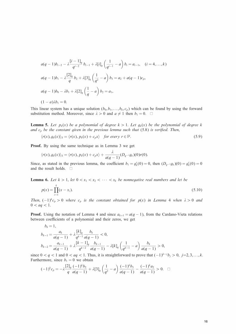
a(q− 1)bi−2 − �[i − 1]qqi−2

bi−1 + �[i]q

(1qi−1

− a)bi = ai−1; (i = 4; : : : ; k)

a(q− 1)b1 − �[2]qqb2 + �[3]q

(1q2

− a)b3 = a2 + a(q− 1)cp;

a(q− 1)b0 − �b1 + �[2]q(1q− a

)b2 = a1;

(1− a)�b1 = 0:This linear system has a unique solution (b0; b1; : : : ; bk ; cp) which can be found by using the forwardsubstitution method. Moreover, since �¿ 0 and a �= 1 then b1 = 0.

Lemma 5. Let pk(x) be a polynomial of degree k ¿ 1. Let gk(x) be the polynomial of degree kand cp be the constant given in the previous lemma such that (5:8) is veri�ed. Then;

〈r(x); gk(x)〉S = 〈r(x); pk(x) + cpx〉 for every r ∈P: (5.9)

Proof. By using the same technique as in Lemma 3 we get

〈r(x); gk(x)〉S = 〈r(x); pk(x) + cpx〉+ �a(q− 1)(Dq−1gk)(0)r(0):

Since, as stated in the previous lemma, the coe�cient b1 = g′k(0) = 0, then (Dq−1gk)(0) = g′k(0) = 0and the result holds.

Lemma 6. Let k ¿ 1; let 0¡x1¡x2¡ · · · ¡xk be nonnegative real numbers and let be

p(x) =k∏i=1

(x − xi): (5.10)

Then; (−1)kcp ¿ 0 where cp is the constant obtained for p(x) in Lemma 4 when �¿ 0 and0¡aq¡ 1.

Proof. Using the notation of Lemma 4 and since ak+1 = a(q− 1); from the Cardano-Vieta relationsbetween coe�cients of a polynomial and their zeros, we get

bk =1;

bk−1 =ak

a(q− 1) + �[k]qqk−1

bka(q− 1)¡ 0;

bk−2 =ak−1

a(q− 1) + �[k − 1]qqk−2

bk−1a(q− 1) − �[k]q

(1qk−1

− a)

bka(q− 1)¿ 0;

since 0¡q¡ 1 and 0¡aq¡ 1. Thus, it is straightforward to prove that (−1)k−jbj ¿ 0; j=2; 3; : : : ; k.Furthermore, since b1 = 0 we obtain

(−1)kcp =−� [2]qq(−1)kb2a(q− 1) + �[3]q

(1q2

− a)(−1)kb3a(q− 1) −

(−1)ka2a(q− 1)¿ 0:

16

Theorem 2. Let {pn(x; a|q)}n be the little q-Laguerre MOPS with 0¡aq¡ 1 and {Qn(x)}n bethe little q-Laguerre–Sobolev MOPS. For each �¿ 0 the polynomial Qn(x); n¿2; has exactly nreal and distinct zeros; where at least n − 1 of them are positive. Moreover; if a61 then all thezeros of Qn(x) are positive. If we denote by xn;1¡xn;2¡ · · · ¡xn;n the zeros of pn(x; a|q) and ifwe denote by yn;1¡yn;2¡ · · · ¡yn;n the n di�erent zeros of Qn(x) then

yn;1¡xn;1¡yn;2¡xn;2¡ · · · ¡yn;n ¡ xn;n: (5.11)

Proof. Assume n¿ 2. Let xn;1¡xn;2¡ · · · ¡xn;n be the zeros of pn(x; a|q) and let us de�ne for16i6n the polynomial w(i)n−1 of degree n− 1 as

w(i)n−1 =n∏

j=1; j �=i(x − xn; j): (5.12)

• If a �= 1 by using Lemma 4 we obtain a unique polynomial g(i)n−1(x) of degree n− 1 as well asa unique constant ci such that (Sg

(i)n−1)(x) = h(x)(w

(i)n−1(x) + cix). From Lemma 5 we get

0 = 〈Qn(x); g(i)n−1(x)〉S = 〈w(i)n−1(x); Qn(x)〉+ ci〈x; Qn(x)〉

=∞∑k=0

w(i)n−1(qk)Qn(qk)�(qk) + ci

∞∑k=0

qkQn(qk)�(qk):

The Gaussian-type quadrature formula based in the zeros of pn(x; a|q) yields

0 = 〈Qn(x); g(i)n−1(x)〉S = �iw(i)n−1(xn; i)Qn(xn; i) + ci∞∑k=0

qkQn(qk)�(qk): (5.13)

Let us compute the second term of the above sum by using (3.5)

ci∞∑k=0

qkQn(qk)�(qk) = ci〈x; Qn(x)〉= cin∑j=1

ej;n〈x; pj(x; a|q)〉= cie1; nk1:

Since k1¿ 0, sgn(e1; n) = (−1)n−2 and sgn(ci) = (−1)n−1, we obtain that the right-hand side of theabove expression is always negative.From (5.13) we deduce

�iw(i)n−1(xn; i)Qn(xn; i) =−ci

∞∑k=0

qkQn(qk)�(qk)¿ 0

and then Qn(xn; i) �= 0. Moreover sgn(Qn(xn; i)) = sgn(w(i)n−1(xn; i)) = (−1)n−i, so Qn(x) changes signbetween two consecutive zeros of pn(x; a|q).Finally, since sgn(Qn(xn;1)) = (−1)n−1 then Qn(x) has n di�erent real zeros, which separate those

of pn(x; a|q) as stated.• If a=1, we use the orthogonality of Qn(x), Lemma 3 and the Gaussian-type quadrature formula

for evaluating sums in order to obtain

0= 〈Qn(x); g(i)n−1(x)〉S = 〈Qn(x); w(i)n−1(x)〉 −�

1− qQn(0)(Dq−1g(i)n−1)(0)

= �iw(i)n−1(xn; i)Qn(xn; i)−

�1− qQn(0)(Dq−1pi)(0) ;

17

where w(i)n−1(x) are the polynomials de�ned in (5.12). Thus,

�iw(i)n−1(xn; i)Qn(xn; i) =

�1− qQn(0)(Dq−1g(i)n−1)(0):

From Lemma 1 and repeating the arguments of Lemma 6 we get (−1)n−2(Dq−1g(i)n−1)(0)¿ 0. Hencewe deduce �iw

(i)n−1(xn; i)Qn(xn; i)¿ 0, and then Qn(xn; i) �= 0 as well as sgn(Qn(xn; i)) = (−1)n−i. The

proof follows in the same way as in the case already discussed.Finally, by Lemma 1, if a61 we have (−1)nQn(0)¿ 0, and all zeros are positive.The result for n= 2 is a consequence of

p2(x; a|q)− Q2(x) = a�q(−1 + q2)(−1 + aq+ x)

�+ a(−1 + q)q(−1 + aq) :

6. Asymptotic properties

In this section asymptotic properties of the sequence {Qn(x)}n on compact subsets of C \ [0; 1]are studied (results on asymptotic properties for polynomials orthogonal with respect to di�erentSobolev inner products have been given in, e.g., [2,16,18,21,26]). More precisely, we shall derive therelative asymptotics {Qn(x)=pn(x; a|q)} and the asymptotic behavior of the ratio of two consecutivelittle q-Laguerre–Sobolev orthogonal polynomials {Qn+1(x)=Qn(x)} on compact subsets of C \ [0; 1].As a consequence, we recover the relative asymptotics between monic Laguerre–Sobolev orthogonalpolynomials {Q()n (x)}n and monic Laguerre orthogonal polynomials {L()n (x)}n given in [17].First, using [32, Theorem 1, p. 263] we can give the ratio asymptotics for little q-Laguerre

polynomials.

Proposition 8. Let {pn(x; a|q)}n be the little q-Laguerre MOPS. The following ratio asymptoticsholds:

limn→∞

pn(x; a|q)pn+1(x; a|q) =

1x; 0¡aq¡ 1 (6.1)

uniformly on compact subsets of C \ [0; 1].

Now, we give bounds for the squared norm kn de�ned in (3.4).

Proposition 9. Let kn and kn given in (2:15) and (3:4); respectively. For n¿1; we have

kn + �([n]q)2kn−16kn6kn + (�([n]q)

2 + (a(1− qn)qn−1)2)kn−1; (6.2)

where [n]q is given in (2:11):

Proof. The inequality on the right-hand side of (6.2) is straightforward from (3.10). Using theextremal property of kn we have, for n¿1,

kn = 〈Qn(x); Qn(x)〉S = 〈Qn(x); Qn(x)〉+ �〈(DqQn)(x); (DqQn)(x)〉¿kn + �([n]q)2kn−1:

18

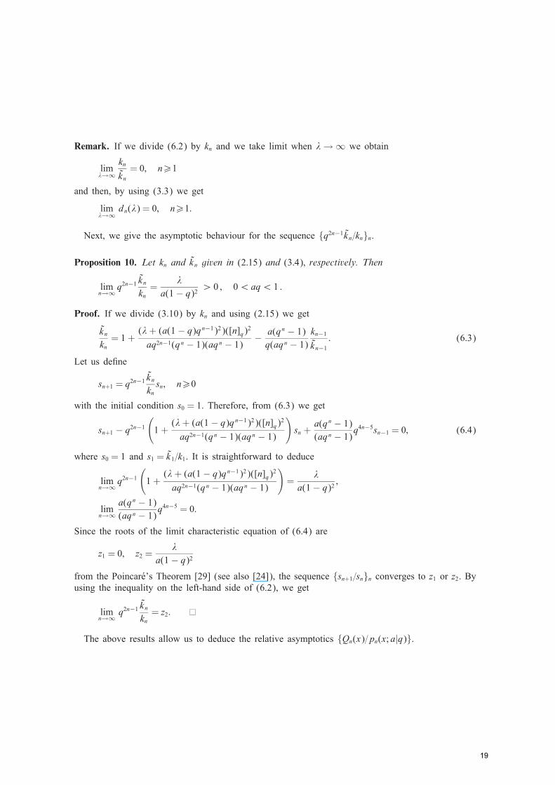
Remark. If we divide (6.2) by kn and we take limit when �→ ∞ we obtain

lim�→∞

knkn= 0; n¿1

and then, by using (3.3) we get

lim�→∞

dn(�) = 0; n¿1:

Next, we give the asymptotic behaviour for the sequence {q2n−1kn=kn}n.

Proposition 10. Let kn and kn given in (2:15) and (3:4); respectively. Then

limn→∞ q

2n−1 knkn=

�a(1− q)2 ¿ 0 ; 0¡aq¡ 1 :

Proof. If we divide (3.10) by kn and using (2.15) we get

knkn= 1 +

(�+ (a(1− q)qn−1)2)([n]q)2aq2n−1(qn − 1)(aqn − 1) − a(qn − 1)

q(aqn − 1)kn−1kn−1

: (6.3)

Let us de�ne

sn+1 = q2n−1knknsn; n¿0

with the initial condition s0 = 1. Therefore, from (6.3) we get

sn+1 − q2n−1(1 +

(�+ (a(1− q)qn−1)2)([n]q)2aq2n−1(qn − 1)(aqn − 1)

)sn +

a(qn − 1)(aqn − 1)q

4n−5sn−1 = 0; (6.4)

where s0 = 1 and s1 = k1=k1. It is straightforward to deduce

limn→∞ q

2n−1(1 +

(�+ (a(1− q)qn−1)2)([n]q)2aq2n−1(qn − 1)(aqn − 1)

)=

�a(1− q)2 ;

limn→∞

a(qn − 1)(aqn − 1)q

4n−5 = 0:

Since the roots of the limit characteristic equation of (6.4) are

z1 = 0; z2 =�

a(1− q)2from the Poincar�e’s Theorem [29] (see also [24]), the sequence {sn+1=sn}n converges to z1 or z2. Byusing the inequality on the left-hand side of (6.2), we get

limn→∞ q2n−1

knkn= z2:

The above results allow us to deduce the relative asymptotics {Qn(x)=pn(x; a|q)}.

19

Theorem 3. Let {Qn(x)}n be the little q-Laguerre–Sobolev MOPS and let {pn(x; a|q)}n be thelittle q-Laguerre MOPS. The following limit relation holds:

limn→∞

Qn(x)pn(x; a|q) = 1; 0¡aq¡ 1 (6.5)

uniformly on compact subsets of C \ [0; 1].

Proof. From (3.2) and (3.3) we can write for n¿1,

1 + a(1− qn)qn−1pn−1(x; a|q)pn(x; a|q) =

Qn(x)pn(x; a|q) + a(1− q

n)qn−1kn−1kn−1

pn−1(x; a|q)pn(x; a|q)

Qn−1(x)pn−1(x; a|q) :

(6.6)

From (6.1) and Proposition 10,

limn→∞ a(1− q

n)qn−1kn−1kn−1

pn−1(x; a|q)pn(x; a|q) = 0 (6.7)

uniformly on compact subsets of C \ [0; 1]. For a �xed compact set K in C \ [0; 1], there existn0 ∈N; j0; j1 ∈R+ such that∣∣∣∣ Qn(x)

pn(x; a|q)∣∣∣∣61 + j0 + j1

∣∣∣∣ Qn−1(x)pn−1(x; a|q)

∣∣∣∣ :Thus, {Qn(x)=pn(x; a|q)}n is uniformly bounded on K . Taking limits in (6.6) when n → ∞, from(6.1) and (6.7) we get the result.

From Theorems 2 and 3 we obtain

Corollary 3. The set of zeros of Qn(x) accumulates on [0; 1]. If a¿ 1; then

limn→∞ yn;1 = 0;

where yn;1¡yn;2¡ · · · ¡yn;n are the zeros of the nth degree monic little q-Laguerre–Sobolevpolynomial Qn(x).

Next, we give the asymptotic behavior of the ratio of two consecutive little q-Laguerre–Sobolevorthogonal polynomials, which is a consequence of Proposition 8 and Theorem 3.

Corollary 4. Let {Qn(x)}n be the little q-Laguerre–Sobolev MOPS. Then

limn→∞

Qn+1(x)Qn(x)

= x (6.8)

uniformly on compact subsets of C\ [0; 1].

Remark. It should be �nally mentioned that we can recover the relative asymptotics between monicLaguerre–Sobolev orthogonal polynomials {Q()n (x)}n and monic Laguerre orthogonal polynomials

20

{L()n (x)}n given in [17]. From (2.12) and (3.2) when a= q we get

pn((1− q)x; q−1|q)=Qn((1− q)x; q; �(1− q)2|q) + dn−1(�(1− q)2; q|q)Qn−1((1− q)x; q; �(1− q)2|q):

If we take the limit in the above expression when q ↑ 1 (see Proposition 3 and (3.11)) we obtainL(−1)n (x) = Q()n (x) + dn−1(�; )Q

()n−1(x); (6.9)

where {L()n (x)}n are the monic Laguerre polynomials, {Q()n (x)}n are the monic Laguerre–Sobolevpolynomials and the coe�cients dn(�; ) are de�ned by means of the recurrence relation given in(3.14). From (6.9), using the same technique as in Theorem 3, it can be deduced that

limn→∞

Q()n (x)

L(−1)n (x)=

2√�2 + 4�− � (6.10)

holds uniformly on compact subsets of C\[0;∞), which is the monic form of the asymptotic behaviorobtained in [17].

Acknowledgements

E.G. wishes to acknowledge partial �nancial support by Direcci�on General de Ensenanza Superior(DGES) of Spain under Grant PB-96-0952. The research of F.M. was partially supported by DGESof Spain under Grant PB96-0120-C03-01 and INTAS Project 93-0219 Ext. J.J.M.B. also wishes toacknowledge partial �nancial support by Junta de Andaluc��a, Grupo de Investigaci�on FQM 0229.

References

[1] I. Area, E. Godoy, F. Marcell�an, Inner products involving di�erences: the Meixner–Sobolev polynomials,J. Di�erence Equations Appl., in print.

[2] I. Area, E. Godoy, F. Marcell�an, J.J. Moreno-Balc�azar, Ratio and Plancherel–Rotach asymptotics for Meixner–Sobolevorthogonal polynomials, J. Comput. Appl. Math. 116 (2000) 63–75.

[3] T.S. Chihara, An Introduction to Orthogonal Polynomials, Gordon and Breach, New York, 1978.[4] W.D. Evans, L.L. Littlejohn, F. Marcell�an, C. Markett, A. Ronveaux, On recurrence relations for Sobolev orthogonal

polynomials, SIAM J. Math. Anal. 26 (2) (1995) 446–467.[5] G. Gasper, M. Rahman, Basic hypergeometric series, Encyclopedia of Mathematics and its Applications,

vol. 35, Cambridge University Press, Cambridge, 1990. Electronic version of errata available athttp:==www.math.nwu.edu/preprints=gasper=bhserrata.

[6] W. Gautschi, M. Zhang, Computing orthogonal polynomials in Sobolev spaces, Numer. Math. 71 (2) (1995)159–183.

[7] W. Hahn, �Uber Orthogonalpolynome, die q-Di�erenzengleichungen gen�ugen, Math. Nach. 2 (1949) 4–34.[8] W. Hahn, �Uber Polynome, die gleichzetig zwei verschiedenen Orthogonalsystemen angeh�oren, Math. Nach. 2 (1949)

263–278.[9] M.E.H. Ismail, M. Rahman, The q-Laguerre polynomials and related moment problems, J. Math. Anal. Appl. 218

(1998) 155–174.[10] F.H. Jackson, On q-de�nite integrals, Quart. J. Pure Appl. Math. 41 (1910) 193–203.[11] R. Koekoek, Generalizations of the classical Laguerre polynomials and some q-analogues, Doctoral Dissertation,

Delft University of Technology, 1990.

21

22 I. Area et al. / Journal of Computational and Applied Mathematics 118 (2000) 1–22

[12] R. Koekoek, Generalizations of the classical Laguerre polynomials and some q-analogues, J. Approx. Theory 69(1992) 55–83.

[13] R. Koekoek, R.F. Swarttouw, The Askey-scheme of hypergeometric orthogonal polynomials and its q-analogue,Reports of the Faculty of Technical Mathematics and Informatics, 98-17, Delft University of Technology, Delft1998.

[14] T.H. Koornwinder, Compact quantum groups and q-special functions, in V. Baldoni, M.A. Picardello (Eds.),Representations of Lie Groups and Quantum Groups, Pitman Research Notes in Mathematics Series, Vol. 311,Longman Scienti�c & Technical, Harlow, 1994, pp. 46–128.

[15] D.C. Lewis, Polynomial least square approximations, Amer. J. Math. 69 (1947) 273–278.[16] G. L�opez, F. Marcell�an, W. van Assche, Relative asymptotics for polynomials with respect to a discrete Sobolev

inner product, Constr. Approx. 11 (1995) 107–137.[17] F. Marcell�an, H.G. Meijer, T.E. P�erez, M.A. Pinar, An asymptotic result for Laguerre–Sobolev orthogonal

polynomials, J. Comput. Appl. Math. 87 (1997) 87–94.[18] F. Marcell�an, J.J. Moreno-Balc�azar, Strong and Plancherel–Rotach asymptotics of non-diagonal Laguerre–Sobolev

polynomials, submitted.[19] F. Marcell�an, T.E. P�erez, M.A. Pinar, Orthogonal polynomials on weighted Sobolev spaces: the semiclassical case,

Ann. Numer. Math. 2 (1995) 93–122.[20] F. Marcell�an, T.E. P�erez, M.A. Pinar, Laguerre–Sobolev orthogonal polynomials, J. Comput. Appl. Math. 71 (1996)

245–265.[21] A. Mart��nez-Finkelshtein, Bernstein–Szeg�o’s theorem for Sobolev orthogonal polynomials, Constr. Approx. 16 (2000)

73–84.[22] J.C. Medem, Polinomios Ortogonales q-semicl�asicos, Doctoral Dissertation, Universidad Polit�ecnica de Madrid, 1996

(in Spanish).[23] J. Meixner, Orthogonale Polynomsysteme mit einer besonderen gestalt der erzeugenden Funktionen, J. London Math.

Soc. 9 (1934) 6–13.[24] L.M. Milne-Thomson, The Calculus of Finite Di�erences, MacMillan, London, 1933.[25] D.S. Moak, The q-analogue of the Laguerre polynomials, J. Math. Anal. Appl. 81 (1981) 20–47.[26] J.J. Moreno-Balc�azar, Propiedades Anal��ticas de los Polinomios Ortogonales de Sobolev Continuos, Doctoral

Dissertation, Universidad de Granada, 1997 (in Spanish).[27] A.F. Nikiforov, S.K. Suslov, V.B. Uvarov, Classical Orthogonal Polynomials of a Discrete Variable, Springer, Berlin,

1991.[28] T.E. P�erez, Polinomios Ortogonales Respecto a Productos de Sobolev: El Caso Continuo, Doctoral Dissertation,

Universidad de Granada, 1994 (in Spanish).[29] H. Poincar�e, Sur les Equations Lin�eaires aux Di��erentielles ordinaires et aux Di��erences �nies, Amer. J. Math. 7

(1885) 203–258.[30] J. Thomae, Beitr�age zur Theorie der durch die Heinesche Reihe; 1 + ((1 − q)(1 − q )=(1 − q)(1 − q�))x + · · ·

darstellbaren funktionen, J. Reine Angew. Math. 70 (1869) 258–281.[31] J. Thomae, Les s�eries Hein�eennes sup�erieures, ou les s�eries de la forme .., Ann. Mat. Pura Appl. 4 (1870) 105–138.[32] W. van Assche, Asymptotic properties of orthogonal polynomials from their recurrence formula, I, J. Approx. Theory

44 (1985) 258–276.

22