Nonlinear Analysis 68 (2008) 1382–1397www.elsevier.com/locate/na

“Bubble-Tower” phenomena in a semilinear elliptic equation withmixed Sobolev growth

Juan F. Campos∗

Departamento de Ingenierıa Matematica, Universidad de Chile, Casilla 170 Correo 3, Santiago, Chile

Received 1 November 2006; accepted 19 December 2006

Abstract

In this work we consider the following problem1u + u p

+ uq= 0 in RN

u > 0 in RN

lim|x |→∞

u(x) → 0

with N/(N − 2) < p < p∗= (N + 2)/(N − 2) < q , N ≥ 3.

We prove that if p is fixed, and q is close enough to the critical exponent p∗, then there exists a radial solution which behaveslike a superposition of bubbles of different blow-up orders centered at the origin. Similarly when q is fixed and p is sufficientlyclose to the critical, we prove the existence of a radial solution which resembles a superposition of flat bubbles centered at theorigin.c© 2007 Elsevier Ltd. All rights reserved.

Keywords: Bubble-Tower phenomena; Lyapunov–Schmidt reduction; Critical exponent

1. Introduction

Let us consider the problem1u + u p

+ uq= 0 in RN

u > 0 in RN

lim|x |→∞

u(x) → 0(1)

∗ Tel.: +56 2 678 0590; fax: +56 2 688 3821.E-mail address: jcampos@dim.uchile.cl.

0362-546X/$ - see front matter c© 2007 Elsevier Ltd. All rights reserved.doi:10.1016/j.na.2006.12.032

J.F. Campos / Nonlinear Analysis 68 (2008) 1382–1397 1383

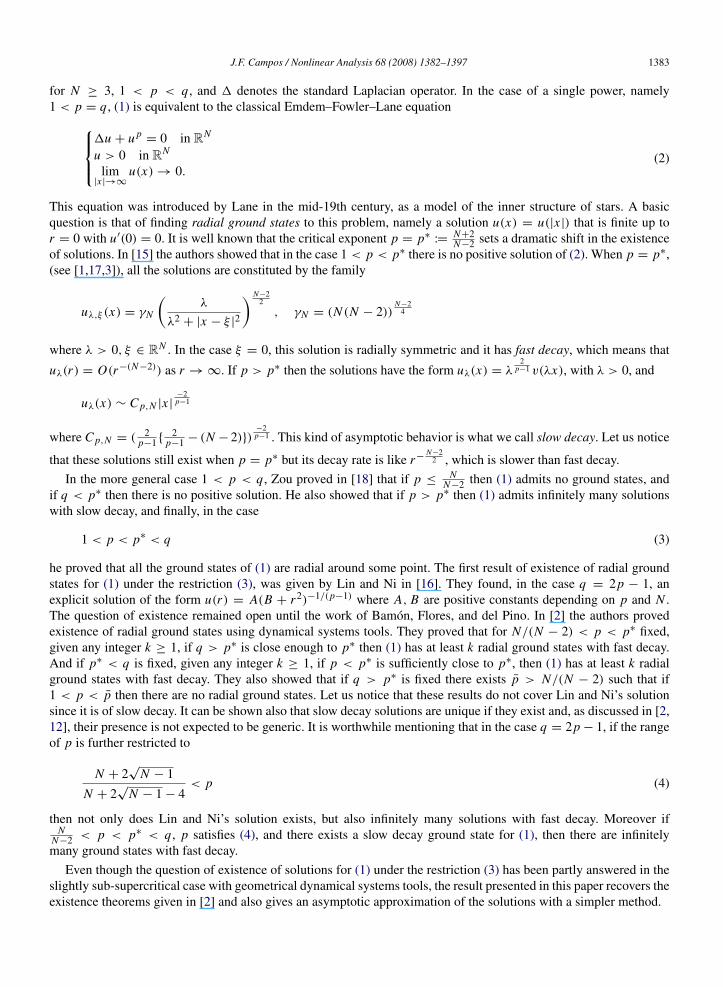
for N ≥ 3, 1 < p < q , and 1 denotes the standard Laplacian operator. In the case of a single power, namely1 < p = q , (1) is equivalent to the classical Emdem–Fowler–Lane equation

1u + u p= 0 in RN

u > 0 in RN

lim|x |→∞

u(x) → 0.(2)

This equation was introduced by Lane in the mid-19th century, as a model of the inner structure of stars. A basicquestion is that of finding radial ground states to this problem, namely a solution u(x) = u(|x |) that is finite up tor = 0 with u′(0) = 0. It is well known that the critical exponent p = p∗

:=N+2N−2 sets a dramatic shift in the existence

of solutions. In [15] the authors showed that in the case 1 < p < p∗ there is no positive solution of (2). When p = p∗,(see [1,17,3]), all the solutions are constituted by the family

uλ,ξ (x) = γN

(λ

λ2 + |x − ξ |2

) N−22

, γN = (N (N − 2))N−2

4

where λ > 0, ξ ∈ RN . In the case ξ = 0, this solution is radially symmetric and it has fast decay, which means that

uλ(r) = O(r−(N−2)) as r → ∞. If p > p∗ then the solutions have the form uλ(x) = λ2

p−1 v(λx), with λ > 0, and

uλ(x) ∼ C p,N |x |−2p−1

where C p,N = ( 2p−1 {

2p−1 − (N − 2)})

−2p−1 . This kind of asymptotic behavior is what we call slow decay. Let us notice

that these solutions still exist when p = p∗ but its decay rate is like r−N−2

2 , which is slower than fast decay.

In the more general case 1 < p < q , Zou proved in [18] that if p ≤N

N−2 then (1) admits no ground states, andif q < p∗ then there is no positive solution. He also showed that if p > p∗ then (1) admits infinitely many solutionswith slow decay, and finally, in the case

1 < p < p∗ < q (3)

he proved that all the ground states of (1) are radial around some point. The first result of existence of radial groundstates for (1) under the restriction (3), was given by Lin and Ni in [16]. They found, in the case q = 2p − 1, anexplicit solution of the form u(r) = A(B + r2)−1/(p−1) where A, B are positive constants depending on p and N .The question of existence remained open until the work of Bamon, Flores, and del Pino. In [2] the authors provedexistence of radial ground states using dynamical systems tools. They proved that for N/(N − 2) < p < p∗ fixed,given any integer k ≥ 1, if q > p∗ is close enough to p∗ then (1) has at least k radial ground states with fast decay.And if p∗ < q is fixed, given any integer k ≥ 1, if p < p∗ is sufficiently close to p∗, then (1) has at least k radialground states with fast decay. They also showed that if q > p∗ is fixed there exists p > N/(N − 2) such that if1 < p < p then there are no radial ground states. Let us notice that these results do not cover Lin and Ni’s solutionsince it is of slow decay. It can be shown also that slow decay solutions are unique if they exist and, as discussed in [2,12], their presence is not expected to be generic. It is worthwhile mentioning that in the case q = 2p − 1, if the rangeof p is further restricted to

N + 2√

N − 1

N + 2√

N − 1 − 4< p (4)

then not only does Lin and Ni’s solution exists, but also infinitely many solutions with fast decay. Moreover ifN

N−2 < p < p∗ < q , p satisfies (4), and there exists a slow decay ground state for (1), then there are infinitelymany ground states with fast decay.

Even though the question of existence of solutions for (1) under the restriction (3) has been partly answered in theslightly sub-supercritical case with geometrical dynamical systems tools, the result presented in this paper recovers theexistence theorems given in [2] and also gives an asymptotic approximation of the solutions with a simpler method.

1384 J.F. Campos / Nonlinear Analysis 68 (2008) 1382–1397

More precisely we prove the existence of a solution which asymptotically resembles a superposition of bubbles ofdifferent blow-up orders, centered at the origin. First we consider the case

1u + u p+ u p∗

+ε= 0 in RN

u > 0 in RN

lim|x |→∞

u(x) → 0(5)

where NN−2 < p is fixed and ε > 0. Then we have

Theorem 1. Let N ≥ 3 and NN−2 < p. Then for any k ∈ N there exists, for all sufficiently small ε > 0, a solution uε

of (5) of the form

uε(y) = γN

k∑i=1

1

1 + α4

N−2i ε

−

(i−1+

1p∗−p

)4

N−2 |y|2

N−22

αiε−

(i−1+

1p∗−p

)(1 + o(1)),

with o(1) → 0 uniformly in RN , as ε → 0. The constants αi can be computed explicitly and depend only on N andp.

This kind of concentration phenomena is known as bubble-tower, and it has been detected for some semilinear ellipticequations with radial symmetry, see for example [6,4,5]. The existence of bubble-tower solutions in the case of ageneric domain has been established for the Brezis–Nirenberg problem in [14], see also [10].

In the case1u + u p∗

−ε+ uq

= 0 in RN

u > 0 in RN

lim|x |→∞

u(x) → 0(6)

with p∗ < q fixed, for any k ∈ N, we prove the existence of a solution which behaves like the superposition of k flatbubbles with a small maximum value which approaches zero uniformly as ε → 0. In [8] the authors detected thesekind of solutions to the problem of finding radially symmetric solutions of the prescribed mean curvature equation.

Theorem 2. Let N ≥ 3 and p∗ < q be fixed. Then given k ∈ N exists, for ε > 0 small enough, a solution uε of theproblem (6) of the form

uε(y) = γN

k∑i=1

1

1 + β4

N−2i ε

(i−1+

1q−p∗

)4

N−2 |y|2

N−22

βiε

(i−1+

1q−p∗

)(1 + o(1))

with o(1) → 0 uniformly on RN , where the constants βi depend only on N y q, can be computed explicitly.

To prove these theorems we use the so-called Emden–Fowler transformation, first introduced in [13], whichconverts dilations into translations, so the problem of finding a k-bubble solution for (1) becomes equivalent tothe problem of finding a k-bump solution of a second-order equation on R. Then a variation of Lyapunov–Schmidtprocedure reduces the construction of these solutions to a finite-dimensional variational problem on R. This kind ofreduction, first introduced in [11], has been used to detect bubbling concentration phenomena in [6,7], and it also canbe adapted to certain situations without radial symmetry, for example when symmetry with respect to N axes at apoint of the domain is assumed, see for example [9,7].

The rest of the paper is organized as follows, the next three sections are devoted to the proof of the Theorem 1:we first state an asymptotical estimate of the energy of the ansatz, which is the key to the method, after that we solvea nonlinear linear problem corresponding to the finite-dimensional reduction, and then solve the finite-dimensionalvariational problem. The last section is the proof of Theorem 2, which is similar to the first one, except for some minorvariations.

J.F. Campos / Nonlinear Analysis 68 (2008) 1382–1397 1385

2. The asymptotic expansion

We are interested in the problem of finding a solution u of (5) with fast decay. We can assume that u is radialaround the origin, and then (5) becomes equivalent to

u′′(r)+N − 1

ru′(r)+ u p(r)+ u p∗

+ε(r) = 0 r ∈ (0,∞)

u′(0) = 0lim

r→∞u(r) → 0.

(7)

Introducing the change of variable

v(x) = r2

p∗−1 u(r) |r=e−

p∗−12 x

(8)

for x ∈ R, which is the so-called Emden–Fowler transformation, the problem (7) becomes{v′′(x)+ β[eεxv p∗

+ε(x)+ e−(p∗−p)xv p(x)] − v = 0 in R

0 < v(x) → 0 as x → ±∞(9)

with β = ( 2N−2 )

2. The functional associated to (9) is

Eε(ψ) = Iε(ψ)−β

p + 1

∫∞

−∞

e−(p∗−p)x

|ψ |p+1dx (10)

where

Iε(ψ) =12

∫∞

−∞

|ψ ′|2dx +

12

∫∞

−∞

|ψ |2dx −

β

p∗ + ε + 1

∫∞

−∞

eεx|ψ |

p∗+ε+1dx .

Let w be the positive radial solution of

1w + w p∗

= 0 in RN

with w(0) = γN , given by u1,0. Now let U be the transformation of w via (8) given by

U (x) = γN e−x (1 + e−(p∗−1)x )−

N−22 . (11)

Then U satisfies{U ′′

− U + βU p∗

= 0 in R0 < U (x) → 0 as |x | → ±∞

(12)

and

γN e−|x |2−N−2

2 ≤ U (x) ≤ γN e−|x |

and therefore U (x) = O(e−|x |).Let us consider 0 < ξ1 < ξ2 < · · · < ξk . We look for a solution of (9) of the form

v(x) =

k∑i=1

U (x − ξi )+ φ

with φ small.We define

Ui (x) = U (x − ξi ), V (x) =

k∑i=1

Ui (x) (13)

1386 J.F. Campos / Nonlinear Analysis 68 (2008) 1382–1397

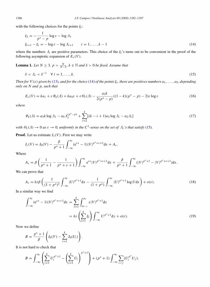
with the following choices for the points ξi :

ξ1 = −1

p∗ − plog ε − log Λ1

ξi+1 − ξi = − log ε − log Λi+1 i = 1, . . . , k − 1 (14)

where the numbers Λi are positive parameters. This choice of the ξi ’s turns out to be convenient in the proof of thefollowing asymptotic expansion of Eε(V ).

Lemma 1. Let N ≥ 3, p > NN−2 , k ∈ N and δ > 0 be fixed. Assume that

δ < Λi < δ−1∀ i = 1, . . . , k. (15)

Then for V (x) given by (13), and for the choice (14) of the points ξi , there are positives numbers a1, . . . , a5, dependingonly on N and p, such that

Eε(V ) = ka1 + εΨk(Λ)+ ka4ε + εΘε(Λ)−a3k

2(p∗ − p)((1 − k)(p∗

− p)− 2)ε log ε (16)

where

Ψk(Λ) = a3k log Λ1 − a5Λ(p∗

−p)1 +

k∑i=2

[(k − i + 1)a3 log Λi − a2Λi ] (17)

with Θε(Λ) → 0 as ε → 0, uniformly in the C1-sense on the set of Λi ’s that satisfy (15).

Proof. Let us estimate Iε(V ). First we may write

Iε(V ) = I0(V )−β

p∗ + 1

∫∞

−∞

(eεx− 1)|V |

p∗+ε+1dx + Aε.

Where

Aε = β

(1

p∗ + 1−

1p∗ + ε + 1

)∫∞

−∞

eεx|V |

p∗+ε+1dx +

β

p∗ + 1

∫∞

−∞

(|V |p∗

+1− |V |

p∗+ε+1)dx .

We can prove that

Aε = kεβ

(1

(1 + p∗)2

∫∞

−∞

|U |p∗

+1dx −1

(1 + p∗)

∫∞

−∞

|U |p∗

+1 log Udx

)+ o(ε). (18)

In a similar way we find∫∞

−∞

(eεx− 1)|V |

p∗+ε+1dx =

k∑l=1

∫ µl

µl−1

x |V |p∗

+1dx

= kε

(k∑

l=1

ξl

)∫∞

−∞

U p∗+1dy + o(ε). (19)

Now we define

B =p∗

+ 1β

(I0(V )−

k∑i=1

I0(Ui )

).

It is not hard to check that

B =

∫∞

−∞

k∑i=1

U p∗+1

i −

(k∑

i=1

Ui

)p∗+1+ (p∗

+ 1)∫

∞

−∞

∑i< j

(U p∗

i U j ).

J.F. Campos / Nonlinear Analysis 68 (2008) 1382–1397 1387

Let us consider

µ0 = −∞, µi =ξi + ξi+1

2i = 1, . . . , k − 1, µk = ∞ (20)

and decompose B as

B =

k∑l=1

(C l1 − C l

0 + C l2)

where

C l0 = (p∗

+ 1)∫ µl

µl−1

U p∗

l

k∑j<l

U j

C l1 =

∫ µl

µl−1

U p∗+1

l −

(k∑

i=1

Ui

)p∗+1

+ (p∗+ 1)U p∗

l

k∑j 6=l

U j

C l

2 =

∫ µl

µl−1

(k∑

i 6=l

U p∗+1

i + (p∗+ 1)

∑i 6=l

∑i< j

U p∗

i U j

).

Now, let us estimate C l1. From the mean value theorem we get

|C l1| ≤ C

∫ µl

µl−1

(k∑

i 6=l

Ui

)2 ( k∑i=1

Ui

)p∗−1

dx .

If l ∈ {2, . . . , k − 1}, setting ρ = − log ε and using the fact that U (x) = O(e−|x |), we get, using (20)

|C l1| ≤ C

∫ ρ2 +K

0e−2|ρ−y|ey(p∗

−1)dy

≤ Ce−2ρ∫ ρ

2 +K

0e−(p∗

−3)ydy = O(e−p∗

+12 ρ) = o(ε)

where K depends only on δ. If l ∈ {1, k}, we easily check that C l1 = o(ε). Similar arguments yield C l

2 = o(ε). Toestimate C l

0, we notice that

C l0 = (p∗

+ 1)∫ µl

µl−1

U p∗

l Ul−1dx + o(ε).

According to (11), we have U (x) = CN cosh(

2xN−2

)−N−2

2, with CN = γN 2−

N−22 . Then

|U (x + ξ)− CN e−|x+ξ || = O(e−p∗

|x+ξ |)

when ξ → ∞. Therefore we obtain

C l0 = (p∗

+ 1)CN eξl−ξl−1

∫∞

−∞

U p∗

(x)ex dx + o(ε).

From these estimates we conclude

I0(V ) = k I0(U )− βCN

∫∞

−∞

U p∗

(x)ex dx

(k∑

l=2

eξl−ξl−1

)+ o(ε). (21)

Finally, we easily check∫∞

−∞

e−(p∗−p)x V p+1(x)dx = e−(p∗

−p)ξ1

∫∞

−∞

e−(p∗−p)xU p+1(x)+ o(ε). (22)

1388 J.F. Campos / Nonlinear Analysis 68 (2008) 1382–1397

Now we define

a1 =12

∫∞

−∞

|U ′(x)|2dx +12

∫∞

−∞

U 2(x)dx −β

p∗ + 1

∫∞

−∞

U p∗+1(x)dx

a2 = βCN

∫∞

−∞

exU p∗

(x)dx

a3 =β

p∗ + 1

∫∞

−∞

U p∗+1(x)dx

a4 =1

(p∗ + 1)2

∫∞

−∞

U p∗+1(x)dx −

1p∗ + 1

∫∞

−∞

U p∗+1(x) log U (x)dx

a5 =β

p + 1

∫∞

−∞

e−(p∗−p)xU p+1(x)dx .

(23)

Collecting the estimates (18)–(22), we get the validity of the following expansion

Eε(V ) = ka1 − a2

k∑l=2

e−(ξl−ξl−1) − εa3

(k∑

i=1

ξi

)+ kεa4 − a5e−(p∗

−p)ξ1 + o(ε).

Using (14), this decomposition reads

Eε(V ) = ka1 + εΨk(Λ)−a3k

2(p∗ − p)((1 − k)(p∗

− p)− 2)ε log ε + ka4ε + o(ε)

with Ψk given by (17). Moreover, the term o(ε) is uniform in the set of the Λi ’s that satisfy (15). The fact thatdifferentiation with respect to Λ leaves o(ε) of the same order follows from very similar computations, so we omitthem. �

Let us notice that the only critical point of Ψk is given by

Λ∗=

([a3k

a5(p∗ − p)

] 1p∗−p

,(k − 1)a3

a2,(k − 2)a3

a2, . . . ,

a3

a2

)and is nondegenerate. This result will be useful since, if V +φ is a solution of (9), with φ small, it is natural to expectthat this only occurs if Λ corresponds to a critical point of Ψk . This is actually true, as we show in the followingsections.

3. The finite-dimensional reduction

In this section we consider p > NN−2 , points 0 < ξ1 < · · · < ξk , which are for now arbitrary, and we keep the

notation V and Ui as in the previous section. We define

Zi (x) = U ′

i (x), i = 1, . . . , k.

Consider the problem of finding a function φ for which there are constants ci , i = 1, . . . , k such thatk∑

i=1

ci Zi = −(V + φ)′′ + (V + φ)− β[eεx (V + φ)

p∗+ε

+ + e−(p∗−p)x (V + φ)

p+

]∫

∞

−∞

Ziφ = 0 ∀i = 1, . . . , k, limx→±∞

φ(x) = 0.

(24)

Let us consider the operator

Lεφ = −φ′′+ φ − β

[(p∗

+ ε)eεx V p∗+ε−1

+ pe−(p∗−p)x V p−1

]φ.

J.F. Campos / Nonlinear Analysis 68 (2008) 1382–1397 1389

The problem (24) gets rewritten asLε(φ) = Nε(φ)+ Rε +

k∑i=1

ci Zi in R∫∞

−∞

Ziφ = 0 ∀i = 1, . . . , k, limx→±∞

φ(x) = 0

(25)

where

Nε(φ) = βeεx ((V + φ)p∗

+ε+ − V p∗

+ε− (p∗

+ ε)V p∗+ε−1φ)+ βe−(p∗

−p)x ((V + φ)p+ − V p

− pV p−1φ)

Rε = β

(eεx V p∗

+ε+ e−(p∗

−p)x V p−

k∑i=1

U p∗

i (x)

).

Next we introduce a convenient functional setting to analyze the invertibility of the operator Lε under the conditionsof orthogonality. For a small σ > 0, to be fixed, and a function ψ : R → R, we define the norm

‖ψ‖∗ = supx∈R

(k∑

i=1

e−σ |x−ξi |

)−1

|ψ(x)|.

To solve (24) it is important first to understand its linear part, where we consider the problem of, given a function h,finding φ such that

Lε(φ) = h +

k∑i=1

ci Zi in R∫∞

−∞

Ziφ = 0 ∀ i = 1, . . . , k, limx→±∞

φ(x) = 0

(26)

for certain constants ci . The following result holds

Proposition 1. There exists positive numbers ε0, δ0, R0 such that, if

R0 < ξ1, R0 < mini=1,...,k

(ξi+1 − ξi ), ξk <δ0

ε(27)

then for all 0 < ε < ε0 and ∀h ∈ C(R) with ‖h‖∗ < ∞, the problem (26) admits a unique solution φ = Tε(h).Besides, there exists C > 0 such that

‖Tε(h)‖∗ ≤ C‖h‖∗, |ci | ≤ C‖h‖∗.

For the proof we need the following,

Lemma 2. Assume that there are sequences εn → 0 and 0 < ξn1 < · · · < ξn

k with

ξn1 → ∞, min

i=1,...,k(ξn

i+1 − ξni ) → ∞, ξn

k = o(ε−1n )

such that for certain functions φn , hn with ‖hn‖∗ → 0, and scalars cni one has

Lεn (φn) = hn +

k∑i=1

cni Zn

i in R∫∞

−∞

Zni φn = 0 ∀ i = 1, . . . , k, lim

x→±∞φn(x) = 0

(28)

with Zni (x) = U ′(x − ξn

i ). Then

limn→∞

‖φn‖∗ = 0.

1390 J.F. Campos / Nonlinear Analysis 68 (2008) 1382–1397

Proof. We will establish first the weaker assertion that

limn→∞

‖φn‖∞ = 0.

By contradiction, we may assume that ‖φn‖∞ = 1. Testing (28) against Znl and integrating by parts we get

k∑i=1

cni

∫∞

−∞

Zni Zn

l dx =

∫∞

−∞

Lεn (Znl )φndx −

∫∞

−∞

hn Znl dx .

This defines an “almost diagonal” system in the cni ’s as n → ∞. Moreover, the fact that Zn

l (x) = O(e−|x−ξnl |),

p > NN−2 , and that Zn

l solves

−Z ′′+ (1 − p∗βU p∗

−1l )Z = 0

yields, after an application of dominated convergence, that limn→∞ cni = 0. If we set xn ∈ RN such that φn(xn) = 1,

we can assume that ∃ i ∈ {1, . . . , k} such that for n large enough

∃ R > 0 such that |xn − ξni | < R. (29)

Let us fix an index i such that (29) holds. We set

φn(x) = φn(x + ξni ).

From (28) and (29) and elliptic estimates, we see that passing to a suitable subsequence φn(x) converges uniformlyover compacts to a nontrivial bounded solution φ of

−φ′′+ φ − βp∗U p∗φ = 0 in R.

Hence φ = cU ′, for some c 6= 0. However

0 =

∫∞

−∞

Znl φn → c

∫∞

−∞

[U ′(x)]2

which is a contradiction. Then necessarily ‖φn‖∞ → 0.Let us observe that (28) takes the form

−φ′′n + φn = gn(x) (30)

with

gn(x) = hn(x)+

k∑i=1

Zni + β[(p∗

+ εn)eεn x V p∗+εn−1

+ pe−(p∗−p)x V p−1

]φn .

If 0 < σ < min{p∗− 1, 1, 2p − 1 − p∗

}, we have

|gn(x)| ≤ θn

k∑i=1

e−σ |x−ξni |

with θn → 0. Choosing c > 0 large enough we get that

ϕn(x) = cθn

k∑i=1

e−σ |x−ξni |

is a supersolution of (30), and −ϕn(x) will be a subsolution of (30). Then

|φn| ≤ θn

k∑i=1

e−σ |x−ξni |

and the proof of the lemma is concluded. �

J.F. Campos / Nonlinear Analysis 68 (2008) 1382–1397 1391

Proof of Proposition 1. Consider

H =

{φ ∈ H1(R) :

∫∞

−∞

Ziφ = 0 ∀i ∈ {1, . . . , k}

}endowed with the inner product [φ,ψ] =

∫∞

−∞(φ′ψ ′

+ φψ). Then the problem (26) expressed in weak form isequivalent to that of finding φ ∈ H such that ∀ψ ∈ H

[φ,ψ] = β

∫∞

−∞

[(p∗

+ ε)eεx V p∗+ε−1

+ pe−(p∗−p)x V p−1

]φψ +

∫∞

−∞

hψ.

With the aid of Riesz representation theorem, this equation gets rewritten in the operational form

[φ,ψ] = [Kε(φ)+ h, ψ]

where h depends linearly on h, and Kε(φ) is compact. Fredholm’s alternative guarantees unique solvability forany h ∈ H , provided that the equation φ = Kε(φ) has only the trivial solution in H . This latter statement holdsfor R0, ε0, δ0 chosen properly, assuming the opposite would lead us to a contradiction with the previous lemma.Continuity can be deduced in a similar way. �

Now we study some differentiability properties of Tε on the variables ξi , that will be important for later purposes.We shall use the notation ξ = (ξ1, . . . , ξk), and consider the Banach space

C∗ = { f ∈ C(R) | ‖ f ‖∗ < ∞}

endowed with the ‖ · ‖∗ norm. We also consider the space L(C∗) of linear operators of C∗.The following result holds.

Proposition 2. Under the assumptions of the Proposition 1, the map ξ → Tε with values in L(C∗) is of class C1.Moreover, there is a constant C > 0 such that

‖DξTε‖L(C∗) ≤ C

uniformly on the vectors ξ that satisfy (27).

Proof. Fix h ∈ C∗, and let φ = Tε(h) for ε < ε0. Consider differentiation with respect to ξl . Let us recall that φsatisfies

Lε(φ) = h +

k∑i=1

ci Zi in R

plus orthogonality conditions, for some constants ci (uniquely determined). For j ∈ {1, . . . , k} we define the constantsα j as the solution of

k∑j=1

α j

∫∞

−∞

Z j Zi = 0 ∀i 6= l

k∑j=1

α j

∫∞

−∞

Z j Zl = −

∫∞

−∞

φ∂ξl Zl .

Again this is an almost diagonal system. We define also the function

f (x) = β∂ξl Fε(x)φ + cl∂ξl Zl −

k∑j=1

α jLε(Z j )

where

Fε(x) = β[(p∗

+ ε)eεx V p∗+ε−1

+ pe−(p∗−p)x V p−1

].

1392 J.F. Campos / Nonlinear Analysis 68 (2008) 1382–1397

Hence ∂ξlφ satisfies

∂ξlφ −

k∑j=1

α j Z j = Tε( f ).

Moreover |αi | ≤ C‖φ‖∗, |ci | ≤ C‖h‖∗, ‖φ‖∗ ≤ C‖h‖∗, so that also ‖∂ξlφ‖∗ ≤ C‖h‖∗ Besides ∂ξlφ dependscontinuously on ξ for this norm, and the validity of the result is proved. �

In what follows we assume, for M > 0 large and fixed, the validity of the constraints

1p∗ − p

log(Mε)−1 < ξ1, log(Mε)−1 < mini=2,...,k

(ξi − ξi−1), ξk < k log(Mε)−1. (31)

For the next purposes it is useful to consider ‖φ‖1 ≤1λ‖V ‖1 where

‖ψ‖1 = supx∈R

(k∑

i=1

e−|x−ξi |

)−1

|ψ |

and λ > 2−N−2

2 . Under these conditions, provided that σ is fixed and small enough, one can easily check that

‖N (φ)‖∗ ≤ C(‖φ‖min{p∗,2}

∗ + ‖φ‖min{2p−p∗,2}

∗ ) (32)∥∥∥∥∂Nε∂φ

∥∥∥∥∗

≤ C(‖φ‖min{p∗

−1,2}

∗ + ‖φ‖min{2p−p∗

−1,2}

∗ ) (33)

and

‖Rε‖∗ ≤ Cεα, ‖∂Rε‖∗ ≤ Cεα (34)

with α =1+λ

2 , for some λ > 0 small enough.

Proposition 3. Assume that conditions (31) hold. Then ∃ C > 0 such that, ∀ε > 0 small enough, there exists a uniquesolution φ = φ(ξ) to the problem (24), which besides satisfies

‖φ‖∗ ≤ Cεα.

Moreover, the map ξ → φ(ξ) is of class C1 for the ‖ · ‖∗-norm, and

‖Dξφ‖∗ ≤ Cεα.

Proof. If we define

Aε(φ) := Tε(Nε(φ)+ Rε)

then (25) is equivalent to the fixed point problem φ = Aε(φ). We will show that Aε is a contraction in a proper region.Let

Fr = {φ ∈ C∗ : ‖φ‖∗ ≤ rεα}

where r > 0 will be fixed later. We have that

‖Aε(φ)‖∗ ≤ ‖Tε (Nε(φ)+ Rε) ‖∗

≤ C‖Nε(φ)+ Rε‖∗

≤ C0((rεα)min{p∗,2}

+ (rεα)min{2p−p∗,2}+ εα).

Besides

|Nε(φ1)− Nε(φ2)| ≤ C((rεα)min{p∗−1,2}

+ (rεα)min{2p−p∗−1,2})|φ1 − φ2|

J.F. Campos / Nonlinear Analysis 68 (2008) 1382–1397 1393

consequently

‖A(φ1)− A(φ2)‖∗ ≤ C1((rεα)min{p∗

−1,2}+ (rεα)min{2p−p∗

−1,2})‖φ1 − φ2‖∗.

If we choose r ≥ 3C0, then for ε small enough

C0((rεα)min{p∗,2}

+ (rεα)min{2p−p∗,2}+ εα) ≤ rεα

C1((rεα)min{p∗

−1,2}+ (rεα)min{2p−p∗

−1,2}) < 1

and so there is a unique fixed point of A in Fr .Concerning now the differentiability of ξ → φ(ξ), let

B(ξ, φ) = φ − Tε(Nε(φ)+ Rε).

Of course we have B(ξ, φ(ξ)) = 0. Now let us write

DφB(ξ, φ)[θ ] = θ − Tε(θDφNε(φ)) = θ + M(θ)

where

M(θ) = −Tε(θDφNε(φ)).

From (33) and using the fact that φ ∈ Fr , we obtain

‖M(θ)‖∗ ≤ C(εαmin{p∗−1,2}

+ εαmin{2p−p∗−1,2})‖θ‖∗.

It follows that for a small ε, the operator DφB(ε, φ) is invertible, with uniformly bounded inverse. It also dependscontinuously on its parameters. Let us differentiate with respect to ξ , we have

Dξ B(ξ, φ) = −DξTε[Nε(φ)+ Rε] − Tε[Dξ Nε(ξ, φ)+ Dξ Rε]

where all these expressions depend continuously on their parameters. Now, the implicit function theorem yields thatφ(ξ) is of class C1 and

Dξφ = −(DφB(ξ, φ)

)−1[Dξ B(ξ, φ)]

so that

‖Dξφ‖∗ ≤ C(‖Nε(φ)+ Rε‖∗ + ‖Dξ Nε(ξ, φ)‖∗ + ‖Dξ Rε‖∗

)≤ Cεα.

This concludes the proof. �

4. The finite-dimensional variational problem

In this section we fix M > 0 large and assume that conditions (31) hold for ξ = (ξ1, . . . , ξk). According to theprevious sections, our original problem has been reduced to that of finding ξ such that the ci that appears in (24),given by Proposition 3, are all zero. Thus we need to solve

ci (ξ) = 0 ∀i ∈ {1, . . . , k}. (35)

This problem is equivalent to a variational problem. We define

Jε(ξ) = Eε(V + φ(ξ)).

Lemma 3. The function V + φ is a solution of (9) ⇔ ξ is a critic point of Jε, where φ = φ(ξ) is given byProposition 3.

Proof. Assume that V + φ solves (9), integrating (9) against ∂ξl (V + φ) we get

DEε(V + φ)∂ξl (V + φ) = 0.

1394 J.F. Campos / Nonlinear Analysis 68 (2008) 1382–1397

Now if ξ is a critic point of Jε, we have

Dξl Jε(ξ) = 0 ⇔ DEε(V + φ)∂ξl (V + φ) = 0

⇔

k∑i=1

ci

∫∞

−∞

Zi∂ξl (V + φ) = 0.

But ∂ξl (V + φ) = Zl + o(1) where o(1) → 0 as ε → 0, uniformly for the ‖ · ‖∗-norm. Therefore

Dξl Jε(ξ) = 0 ∀l = 1, . . . , k ⇔

k∑i=1

ci

∫∞

−∞

Zi [Zl + o(1)] = 0 ∀l = 1, . . . , k

which defines an almost diagonal linear system on ci , and the conclusion follows. �

The next lemma is crucial to find the critical points of Jε.

Lemma 4. The following expansion holds

Jε(ξ) = Eε(V )+ o(ε)

where o(ε) is uniform in the C1-sense on the vectors ξ which satisfy (31).

Proof. Using the fact that DEε(V + φ)[φ] = 0, a Taylor expansion gives

Eε(V + φ)− Eε(V ) =

∫ 1

0D2 Eε(V + tφ)[φ2

]tdt

=

∫ 1

0

∫∞

−∞

(Nε(φ)+ Rε)φtdt

+β(p∗+ ε)

∫ 1

0

∫∞

−∞

eεx[V p∗

+ε−1− (V + tφ)p∗

+ε−1]φ2tdt

+βp∫ 1

0

∫∞

−∞

e−(p∗−p)x

[V p−1

− (V + tφ)p−1]φ2tdt

and since ‖φ‖∗ ≤ Cεα , with α =1+λ

2 , we get

Jε(ξ)− Eε(V ) = O(ε1+λ)

uniformly on the points satisfying (31). Differentiating now with respect to the ξ variables, we obtain

∂ξl (Jε(ξ)− Eε(V )) =

∫ 1

0

∫∞

−∞

∂ξl [(Nε(φ)+ Rε)φ]tdt

+β(p∗+ ε)

∫ 1

0

∫∞

−∞

eεx∂ξl

([V p∗

+ε−1− (V + tφ)p∗

+ε−1]φ2)

tdt

+βp∫ 1

0

∫∞

−∞

e−(p∗−p)x∂ξl

([V p−1

− (V + tφ)p−1]φ2)

tdt.

And from the computations made in the previous propositions we deduce

∂ξl (Jε(ξ)− Eε(V )) = O(ε1+λ)

which concludes the proof. �

Proof of Theorem 1. We consider the change of variable

ξ1 = −1

p∗ − plog ε − log Λ1

ξi+1 − ξi = − log ε − log Λi ∀i ≥ 2

J.F. Campos / Nonlinear Analysis 68 (2008) 1382–1397 1395

where the Λi ’s are positive parameters. For notational convenience, we set Λ = (Λ1, . . . ,Λk). Hence it suffices to findcritical points of

Φε(Λ) = ε−1 Jε(ξ(Λ)).

From the previous lemma and the expansion given in Lemma 1, we get

∇Φε(Λ) = ∇Ψk(Λ)+ o(1)

where o(1) → 0 uniformly on the vectors Λ satisfying M−1 < Λi < M for any fixed large M . As we pointed outbefore, Ψk has only one critical point that we denote Λ∗. Since this critical point is nondegenerate, it follows that thelocal degree deg(∇Φε,U, 0) is well defined and is nonzero. Here U denotes an arbitrarily small neighborhood of Λ∗.Hence for a sufficiently small ε

deg(Jε,U, 0) 6= 0.

We conclude that there exists a critical point Λ∗ε of Φε such that

Λ∗ε = Λ∗

+ o(1).

Then for ξ∗= ξ(Λ∗) we obtain that

v∗=

k∑i=1

U (x − ξi (Λ∗ε))+ φ(ξ(Λ∗

ε)) =

k∑i=1

U (x − ξ∗

i )(1 + o(1))

is a solution of (9), and going back in the transformation (8) we obtain that

u∗ε(r) = γN

k∑i=1

eξ∗i

(1

1 + e(p∗−1)ξ∗

i r2

) N−22

(1 + o(1))

is a solution of (5), where

eξ∗i = ε

−(i−1)− 1p∗−p

i∏j=1

(Λ∗

i )−1

and setting αi = 5ij=1(Λ

∗

i )−1, then

αi =

[a5(p∗

− p)

a3k

] 1p∗−p

(a2

a3

)i−1(k − i)!

(k − 1)!

where the constants a2, a3, a5, are given by (23). �

5. Proof of Theorem 2

In this section we consider the transformation

v(x) = r2

p∗−1 u(r) |r=e

p∗−12 x

(36)

and then problem (6) turns out to be equivalent to{v′′(x)+ β[eεxv p∗

−ε(x)+ e−(q−p∗)xvq(x)] − v = 0 in R0 < v(x) → 0 as x → ±∞.

(37)

The associated functional reads

Eε(ψ) =12

∫∞

−∞

|ψ ′|2dx +

12

∫∞

−∞

|ψ |2dx −

β

p∗ − ε + 1

∫∞

−∞

eεx|ψ |

p∗−ε+1dx

−β

q + 1

∫∞

−∞

e−(q−p∗)x|ψ |

q+1dx . (38)

1396 J.F. Campos / Nonlinear Analysis 68 (2008) 1382–1397

We define U as the transformation via (36) of w, and for small ε > 0 we define

ξ1 = −1

q − p∗log ε − log Λ1

ξi+1 − ξi = − log ε − log Λi+1 i = 1, . . . , k − 1 (39)

where the points Λi are positive parameters. We look for a solution of (37) of the form

v(x) =

k∑i=1

U (x − ξi )+ φ

where φ is small. In a similar way to the proof of Lemma 1, we can prove that for N ≥ 3, k ∈ N, q > p∗ and δ > 0fixed, if

δ < Λi < δ−1∀i = 1, . . . , k (40)

then there are constants b1, . . . , bn depending only on N and q, such that

Eε(V ) = kb1 + εΨk(Λ)− kb4ε + εΘε(Λ)−b3k

2(q − p∗)((1 − k)(q − p∗)− 2)ε log ε (41)

where Λ = (Λ1, . . . , Λk) and

Ψk(Λ) = b3k log Λ1 − b5Λ(q−p∗)

1 +

k∑i=2

[(k − i + 1)b3 log Λi − b2Λi ] (42)

with Θε(Λ) → 0 as ε → 0, uniformly in the C1-sense on the points Λi that satisfy (40). Besides the constants aregiven by

b1 =12

∫∞

−∞

|U ′(x)|2dx +12

∫∞

−∞

U 2(x)dx −β

p∗ + 1

∫∞

−∞

U p∗+1(x)dx

b2 = βCN

∫∞

−∞

exU p∗

(x)dx

b3 =β

p∗ + 1

∫∞

−∞

U p∗+1(x)dx

b4 =1

(p∗ + 1)2

∫∞

−∞

U p∗+1(x)dx −

1p∗ + 1

∫∞

−∞

U p∗+1(x) log U (x)dx

b5 =β

q + 1

∫∞

−∞

e−(q−p∗)xU q+1(x)dx .

(43)

It follows that the only critical point of Ψk is nondegenerate and is given by

Λ∗=

([b3k

b5(q − p∗)

] 1q−p∗

,(k − 1)b3

b2,(k − 2)b3

b2, . . . ,

b3

b2

).

The finite-dimensional reduction can be worked in a way similar to the Section 3, except for (32) and (33), that getreplaced by

‖N (φ)‖∗ ≤ C(‖φ‖min{p∗,2}

∗ + ‖φ‖min{

p∗+12 , 3

2 }

∗ ) (44)∥∥∥∥∂Nε∂φ

∥∥∥∥∗

≤ C(‖φ‖min{p∗

−1,2}

∗ + ‖φ‖min{

p∗−12 ,2}

∗ ). (45)

The finite-dimensional variational problem and the conclusion of the theorem can be derived in a way analogous tothe Section 4. �

J.F. Campos / Nonlinear Analysis 68 (2008) 1382–1397 1397

Acknowledgments

I would like to thank Manuel del Pino for presenting me with the problem, and also Ignacio Guerra for very usefulsuggestions.

References

[1] T. Aubin, Problemes isoperimetriques et espaces de Sobolev, J. Differential Geom. 11 (4) (1976) 573–598.[2] R. Bamon, M. del Pino, I. Flores, Ground states of semilinear elliptic equations: A geometric approach, Ann. Inst. H. Poincare 17 (5) (2000)

551–581.[3] L.A. Caffarelli, B. Gidas, J. Spruck, Asymptotic symmetry and local behavior of semilinear elliptic equations involving critical Sobolev

growth, Comm. Pure Appl. Math. 42 (3) (1989) 271–297.[4] C.C. Chen, C.-S. Lin, Blowing up with infinite energy of conformal metrics on Sn , Comm. Partial Differential Equations 24 (5–6) (1999)

785–799.[5] A. Contreras, M. del Pino, Nodal Bubble-Tower solutions to radial elliptic problems near criticality, Discrete Contin. Dyn. Syst. 16 (3) (2006)

525–539.[6] M. del Pino, J. Dolbeault, M. Musso, “Bubble-Tower” radial solutions in the slightly super critical Brezis–Nirenberg problem, J. Differential

Equations 193 (2) (2003) 280–306.[7] M. del Pino, J. Dolbeault, M. Musso, The Brezis–Nirenberg problem near criticality in dimension 3, J. Math. Pures Appl. (9) 83 (12) (2004)

1405–1456.[8] M. del Pino, I. Guerra, Ground states of a prescribed curvature equation (preprint).[9] M. del Pino, M. Musso, A. Pistoia, Super critical boundary bubbling in a semilinear Neumann problem, Ann. Inst. H. Poincare 22 (1) (2005)

45–82.[10] V. Felli, S. Terracini, Fountain-like solutions for nonlinear equations with critical Hardy potential, Commun. Contemp. Math. 7 (6) (2005)

867–904.[11] A. Floer, A. Weinstein, Nonspreading wave packets for the cubic Schrodinger equation with bounded potential, J. Funct. Anal. 69 (3) (1986)

397–408.[12] I. Flores, A resonance phenomenon for ground states of an elliptic equation of Emden–Fowler type, J. Differential Equations 198 (1) (2004)

1–15.[13] R.H. Fowler, Further studies on Emdens and similar differential equations, Q. J. Math. 2 (1931) 259–288.[14] Y. Ge, R. Jing, F. Pacard, Bubble Towers for supercritical semilinear elliptic equations, J. Funct. Anal. 221 (2) (2005) 251–302.[15] B. Gidas, J. Spruck, A priori bounds for positive solutions of nonlinear elliptic equations, Comm. Partial Differential Equations 6 (8) (1981)

883–901.[16] C.-S. Lin, W.-M. Ni, A counterexample to the nodal line conjecture and a related semilinear equation, Proc. Amer. Math. Soc. 102 (2) (1988)

271–277.[17] G. Talenti, Best constant in Sobolev inequality, Ann Mat. Pura Appl. 110 (4) (1976) 353–372.[18] H. Zou, Symmetry of ground states of semilinear elliptic equations with mixed Sobolev growth, Indiana Univ. Math. J. 45 (1) (1996) 221–240.