Numerical Blow-Up Time for a Semilinear Parabolic Equation with Nonlinear Boundary Conditions
30
Hindawi Publishing Corporation Journal of Applied Mathematics Volume 2008, Article ID 753518, 29 pages doi:10.1155/2008/753518 Research Article Numerical Blow-Up Time for a Semilinear Parabolic Equation with Nonlinear Boundary Conditions Louis A. Assal ´ e, 1 Th ´ eodore K. Boni, 1 and Diabate Nabongo 2 1 Institut National Polytechnique Houphou¨ et-Boigny de Yamoussoukro, BP 1093, Yamoussoukro, Cote D’Ivoire 2 D´ epartement de Math´ ematiques et Informatiques, Universit´ e d’Abobo-Adjam´ e, UFR-SFA, 16 BP 372 Abidjan 16, Cote D’Ivoire Correspondence should be addressed to Diabate Nabongo, nabongo [email protected] Received 29 April 2008; Revised 15 December 2008; Accepted 29 December 2008 Recommended by Jacek Rokicki We obtain some conditions under which the positive solution for semidiscretizations of the semilinear equation u t u xx − ax, tf u, 0 <x< 1,t ∈ 0,T , with boundary conditions u x 0,t 0, u x 1,t btgu1,t, blows up in a finite time and estimate its semidiscrete blow-up time. We also establish the convergence of the semidiscrete blow-up time and obtain some results about numerical blow-up rate and set. Finally, we get an analogous result taking a discrete form of the above problem and give some computational results to illustrate some points of our analysis. Copyright q 2008 Louis A. Assal´ e et al. This is an open access article distributed under the Creative Commons Attribution License, which permits unrestricted use, distribution, and reproduction in any medium, provided the original work is properly cited. 1. Introduction In this paper, we consider the following boundary value problem: u t − u xx −ax, tf u, 0 <x< 1,t ∈ 0,T , u x 0,t 0, u x 1,t btg ( u1,t ) , t ∈ 0,T , ux, 0 u 0 x ≥ 0, 0 ≤ x ≤ 1, 1.1 where f : 0, ∞ → 0, ∞ is a C 1 function, f 0 0, g : 0, ∞ → 0, ∞ is a C 1 convex function, g 0 0, a ∈ C 0 0, 1 × R , ax, t ≥ 0 in 0, 1 × R , a t x, t ≤ 0 in 0, 1 × R , b ∈ C 1 R , bt > 0 in R , b t ≥ 0 in R . The initial data u 0 ∈ C 2 0, 1, u 0 0 0, u 0 1 b1g u 0 1.
-
Upload
independent -
Category
Documents
-
view
0 -
download
0
Transcript of Numerical Blow-Up Time for a Semilinear Parabolic Equation with Nonlinear Boundary Conditions

Hindawi Publishing CorporationJournal of Applied MathematicsVolume 2008, Article ID 753518, 29 pagesdoi:10.1155/2008/753518
Research ArticleNumerical Blow-Up Time for a Semilinear ParabolicEquation with Nonlinear Boundary Conditions
Louis A. Assale,1 Theodore K. Boni,1 and Diabate Nabongo2
1 Institut National Polytechnique Houphouet-Boigny de Yamoussoukro, BP 1093,Yamoussoukro, Cote D’Ivoire
2 Departement de Mathematiques et Informatiques, Universite d’Abobo-Adjame, UFR-SFA,16 BP 372 Abidjan 16, Cote D’Ivoire
Correspondence should be addressed to Diabate Nabongo, nabongo [email protected]
Received 29 April 2008; Revised 15 December 2008; Accepted 29 December 2008
Recommended by Jacek Rokicki
We obtain some conditions under which the positive solution for semidiscretizations of thesemilinear equation ut = uxx − a(x, t)f(u), 0 < x < 1, t ∈ (0, T), with boundary conditionsux(0, t) = 0, ux(1, t) = b(t)g(u(1, t)), blows up in a finite time and estimate its semidiscrete blow-uptime. We also establish the convergence of the semidiscrete blow-up time and obtain some resultsabout numerical blow-up rate and set. Finally, we get an analogous result taking a discrete form ofthe above problem and give some computational results to illustrate some points of our analysis.
Copyright q 2008 Louis A. Assale et al. This is an open access article distributed under theCreative Commons Attribution License, which permits unrestricted use, distribution, andreproduction in any medium, provided the original work is properly cited.
1. Introduction
In this paper, we consider the following boundary value problem:
ut − uxx = −a(x, t)f(u), 0 < x < 1, t ∈ (0, T),
ux(0, t) = 0, ux(1, t) = b(t)g(u(1, t)
), t ∈ (0, T),
u(x, 0) = u0(x) ≥ 0, 0 ≤ x ≤ 1,
(1.1)
where f : [0,∞) → [0,∞) is a C1 function, f(0) = 0, g : [0,∞) → [0,∞) is a C1 convexfunction, g(0) = 0, a ∈ C0([0, 1] × R+), a(x, t) ≥ 0 in [0, 1] × R+, at(x, t) ≤ 0 in [0, 1] × R+,b ∈ C1(R+), b(t) > 0 in R+, b′(t) ≥ 0 in R+. The initial data u0 ∈ C2([0, 1]), u′0(0) = 0, u′0(1) =b(1)g(u0(1)).
2 Journal of Applied Mathematics
Here (0, T) is the maximal time interval on which the solution u of (1.1) exists. Thetime T may be finite or infinite. Where T is infinite, we say that the solution u exists globally.When T is finite, the solution u develops a singularity in a finite time, namely
limt→ T
∥∥u(·, t)
∥∥∞ = +∞, (1.2)
where ‖u(·, t)‖∞ = max0≤x≤1|u(x, t)|.In this last case, we say that the solution u blows up in a finite time and the time T is
called the blow-up time of the solution u.In good number of physical devices, the boundary conditions play a primordial role
in the progress of the studied processes. It is the case of the problem described in (1.1)which can be viewed as a heat conduction problem where u stands for the temperature,and the heat sources are prescribed on the boundaries. At the boundary x = 0, the heatsource has a constant flux whereas at the boundary x = 1, the heat source has a nonlinearradition haw. Intensification of the heat source at the boundary x = 1 is provided by thefunction b. The function g also gives a dominant strength of the heat source at the boundaryx = 1.
The theoretical study of blow-up of solutions for semilinear parabolic equations withnonlinear boundary conditions has been the subject of investigations of many authors (see[1–7], and the references cited therein).
The authors have proved that under some assumptions, the solution of (1.1) blowsup in a finite time and the blow-up time is estimated. It is also proved that under someconditions, the blow-up occurs at the point 1. In this paper, we are interested in the numericalstudy. We give some assumptions under which the solution of a semidiscrete form of (1.1)blows up in a finite time and estimate its semidiscrete blow-up time. We also show that thesemidiscrete blow-up time converges to the theoretical one when the mesh size goes to zero.An analogous study has been also done for a discrete scheme. For the semidiscrete scheme,some results about numerical blow-up rate and set have been also given. A similar studyhas been undertaken in [8, 9] where the authors have considered semilinear heat equationswith Dirichlet boundary conditions. In the same way in [10] the numerical extinction hasbeen studied using some discrete and semidiscrete schemes (a solution u extincts in a finitetime if it reaches the value zero in a finite time). Concerning the numerical study withnonlinear boundary conditions, some particular cases of the above problem have been treatedby several authors (see [11–15]). Generally, the authors have considered the problem (1.1) inthe case where a(x, t) = 0 and b(t) = 1. For instance in [15], the above problem has beenconsidered in the case where a(x, t) = 0 and b(t) = 1. In [16], the authors have consideredthe problem (1.1) in the case where a(x, t) = λ > 0, b(t) = 1, f(u) = up, g(u) = uq. They haveshown that the solution of a semidiscrete form of (1.1) blows up in a finite time and theyhave localized the blow-up set. One may also find in [17–22] similar studies concerning otherparabolic problems.
The paper is organized as follows. In the next section, we present a semidiscretescheme of (1.1). In Section 3, we give some properties concerning our semidiscrete scheme. InSection 4, under some conditions, we prove that the solution of the semidiscrete form of (1.1)blows up in a finite time and estimate its semidiscrete blow-up time. In Section 5, we studythe convergence of the semidiscrete blow-up time. In Section 6, we give some results on thenumerical blow-up rate and Section 7 is consecrated to the study of the numerical blow-up

Louis A. Assale et al. 3
set. In Section 8, we study a particular discrete form of (1.1). Finally, in the last section, takingsome discrete forms of (1.1), we give some numerical experiments.
2. The semidiscrete problem
Let I be a positive integer and define the grid xi = ih, 0 ≤ i ≤ I, where h = 1/I. Weapproximate the solution u of (1.1) by the solution Uh(t) = (U0(t), U1(t), . . . , UI(t))
T of thefollowing semidiscrete equations
dUi(t)dt
− δ2Ui(t) = −ai(t)f(Ui(t)
), 0 ≤ i ≤ I − 1, t ∈
(0, Thb
), (2.1)
dUI(t)dt
− δ2UI(t) =2hb(t)g
(UI(t)
)− aI(t)f
(UI(t)
), t ∈
(0, Thb
), (2.2)
Ui(0) = ϕi ≥ 0, 0 ≤ i ≤ I, (2.3)
where ϕi+1 ≥ ϕi, 0 ≤ i ≤ I − 1,
δ2U0(t) =2U1(t) − 2U0(t)
h2, δ2UI(t) =
2UI−1(t) − 2UI(t)h2
,
δ2Ui(t) =Ui+1(t) − 2Ui(t) +Ui−1(t)
h2.
(2.4)
Here (0, Thb ) is the maximal time interval on which ‖Uh(t)‖∞ is finite where ‖Uh(t)‖∞ =max0≤i≤IUi(t). When Thb is finite, we say that the solution Uh(t) blows up in a finite timeand the time Th
bis called the blow-up time of the solution Uh(t).
3. Properties of the semidiscrete scheme
In this section, we give some lemmas which will be used later.The following lemma is a semidiscrete form of the maximum principle.
Lemma 3.1. Let ah(t) ∈ C0([0, T),RI+1) and let Vh(t) ∈ C1([0, T),RI+1) such that
dVi(t)dt
− δ2Vi(t) + ai(t)Vi(t) ≥ 0, 0 ≤ i ≤ I, t ∈ (0, T),
Vi(0) ≥ 0, 0 ≤ i ≤ I.(3.1)
Then we have Vi(t) ≥ 0, 0 ≤ i ≤ I, t ∈ (0, T).
Proof. Let T0 < T and define the vector Zh(t) = eλtVh(t) where λ is large enough that ai(t)−λ >0 for t ∈ [0, T0], 0 ≤ i ≤ I. Let m = min0≤i≤I, 0≤t≤T0Zi(t). Since for i ∈ {0, . . . , I}, Zi(t) is acontinuous function, there exists t0 ∈ [0, T0] such that m = Zi0(t0) for a certain i0 ∈ {0, . . . , I}.

4 Journal of Applied Mathematics
It is not hard to see that
dZi0
(t0)
dt= lim
k→ 0
Zi0
(t0)− Zi0
(t0 − k
)
k≤ 0,
δ2Zi0
(t0)=Zi0+1
(t0)− 2Zi0
(t0)+ Zi0−1
(t0)
h2≥ 0 if 1 ≤ i0 ≤ I − 1,
δ2Zi0
(t0)=
2Z1(t0)− 2Z0
(t0)
h2≥ 0 if i0 = 0,
δ2Zi0
(t0)=
2ZI−1(t0)− 2ZI
(t0)
h2≥ 0 if i0 = I.
(3.2)
A straightforward computation reveals that
dZi0
(t0)
dt− δ2Zi0
(t0)+(ai0
(t0)− λ
)Zi0
(t0)≥ 0. (3.3)
We observe from (3.2) that (ai0(t0) − λ)Zi0(t0) ≥ 0 which implies that Zi0(t0) ≥ 0 becauseai0(t0) − λ > 0. We deduce that Vh(t) ≥ 0 for t ∈ [0, T0] and the proof is complete.
Another form of the maximum principle for semidiscrete equations is the followingcomparison lemma.
Lemma 3.2. Let Vh(t),Uh(t) ∈ C1([0, T),RI+1) and f ∈ C0(R × R,R) such that for t ∈ (0, T)
dVi(t)dt
− δ2Vi(t) + f(Vi(t), t
)<dUi(t)dt
− δ2Ui(t) + f(Ui(t), t
), 0 ≤ i ≤ I, (3.4)
Vi(0) < Ui(0), 0 ≤ i ≤ I. (3.5)
Then we have Vi(t) < Ui(t), 0 ≤ i ≤ I, t ∈ (0, T).
Proof. Define the vector Zh(t) = Uh(t) − Vh(t). Let t0 be the first t ∈ (0, T) such that Zi(t) > 0for t ∈ [0, t0), 0 ≤ i ≤ I, but Zi0(t0) = 0 for a certain i0 ∈ {0, . . . , I}. We observe that
dZi0
(t0)
dt= lim
k→ 0
Zi0
(t0)− Zi0
(t0 − k
)
k≤ 0,
δ2Zi0
(t0)=Zi0+1
(t0)− 2Zi0
(t0)+ Zi0−1
(t0)
h2≥ 0 if 1 ≤ i0 ≤ I − 1,
δ2Zi0
(t0)=
2Z1(t0)− 2Z0
(t0)
h2≥ 0 if i0 = 0,
δ2Zi0
(t0)=
2ZI−1(t0)− 2ZI
(t0)
h2≥ 0 if i0 = I,
(3.6)
Louis A. Assale et al. 5
which implies that
dZi0
(t0)
dt− δ2Zi0
(t0)+ f
(Ui0
(t0), t0
)− f
(Vi0
(t0), t0
)≤ 0. (3.7)
But this inequality contradicts (3.4) and the proof is complete.
4. Semidiscrete blow-up solutions
In this section under some assumptions, we show that the solution Uh of (2.1)–(2.3) blowsup in a finite time and estimate its semidiscrete blow-up time.
Before starting, we need the following two lemmas. The first lemma gives a propertyof the operator δ2 and the second one reveals a property of the semidiscrete solution.
Lemma 4.1. LetUh ∈ RI+1 be such thatUh ≥ 0. Then we have
δ2g(Ui
)≥ g ′
(Ui
)δ2Ui for 0 ≤ i ≤ I. (4.1)
Proof. Apply Taylor’s expansion to obtain
g(U1
)= g
(U0
)+(U1 −U0
)g ′(U0
)+
(U1 −U0
)2
2g ′′
(η0),
g(Ui+1
)= g
(Ui
)+(Ui+1 −Ui
)g ′(Ui
)+
(Ui+1 −Ui
)2
2g ′′
(θi), 1 ≤ i ≤ I − 1,
g(Ui−1
)= g
(Ui
)+(Ui−1 −Ui
)g ′(Ui
)+
(Ui−1 −Ui
)2
2g ′′
(ηi), 1 ≤ i ≤ I − 1,
g(UI−1
)= g
(UI
)+(UI−1 −UI
)g ′(UI
)+
(UI−1 −UI
)2
2g ′′
(ηI),
(4.2)
where θi is an intermediate between Ui and Ui+1 and ηi the one between Ui−1 and Ui. Thefirst and last equalities imply that
δ2g(U0
)= g ′
(U0
)δ2U0 +
(U1 −U0
)2
h2g ′′
(η0),
δ2g(UI
)= g ′
(UI
)δ2UI +
(UI−1 −UI
)2
h2g ′′
(ηI).
(4.3)
Combining the second and third equalities, we see that
δ2g(Ui
)= g ′
(Ui
)δ2Ui +
(Ui+1 −Ui
)2
2h2g ′′
(θi)+
(Ui−1 −Ui
)2
2h2g ′′
(ηi), 1 ≤ i ≤ I − 1. (4.4)
Use the fact that g ′′(s) ≥ 0 for s ≥ 0 and Uh ≥ 0 to complete the rest of the proof.
6 Journal of Applied Mathematics
Lemma 4.2. LetUh be the solution of (2.1)–(2.3). Then we have
Ui+1(t) > Ui(t), 0 ≤ i ≤ I − 1, t ∈(0, Thb
). (4.5)
Proof. Let t0 be the first t > 0 such that Ui+1(t) > Ui(t) for 0 ≤ i ≤ I − 1 but Ui0+1(t0) = Ui0(t0)for a certain i0 ∈ {0, . . . , I − 1}. Without loss of generality, we may suppose that i0 is thesmallest integer which satisfies the equality. Introduce the functions Zi(t) = Ui+1(t)−Ui(t) for0 ≤ i ≤ I − 1. We get
dZi0
(t0)
dt= lim
k→ 0
Zi0
(t0)− Zi0
(t0 − k
)
k≤ 0,
δ2Zi0
(t0)=Zi0+1
(t0)− 2Zi0
(t0)+ Zi0−1
(t0)
h2> 0 if 1 ≤ i0 ≤ I − 2,
δ2Zi0
(t0)= δ2Z0
(t0)=Z1
(t0)− 3Z0
(t0)
h2> 0 if i0 = 0,
δ2Zi0
(t0)= δ2ZI−1
(t0)=ZI−2
(t0)− 3ZI−1
(t0)
h2> 0 if i0 = I − 1,
(4.6)
which implies that
dZi0
(t0)
dt− δ2Zi0
(t0)− ai0+1
(t0)f(Ui0+1(t0
))
+ ai0(t0)f(Ui0
(t0))
< 0 if 0 ≤ i0 ≤ I − 2,
dZi0
(t0)
dt− δ2Zi0
(t0)+
2hb(t0)gi0+1
(t0)− ai0+1
(t0)f(Ui0+1(t0
))
+ ai0(t0)f(Ui0
(t0))
< 0 if i0 = I − 1.
(4.7)
But this contradicts (2.1)-(2.2) and we have the desired result.
The above lemma says that the semidiscrete solution is increasing in space. Thisproperty will be used later to show that the semidiscrete solution attains its minimum atthe last node xI .
Now, we are in a position to state the main result of this section.
Theorem 4.3. Let Uh be the solution of (2.1)–(2.3). Suppose that there exists a positive integer Asuch that
δ2ϕi − ai(0)f(ϕi)≥ 0, 1 ≤ i ≤ I − 1,
δ2ϕI − aI(0)f(ϕI
)+ b(0)gI
(ϕI
)≥ Ag
(ϕI
).
(4.8)
Assume that
f(s)g ′(s) − f ′(s)g(s) ≥ 0 for s ≥ 0. (4.9)
Louis A. Assale et al. 7
Then the solutionUh blows up in a finite time Thb and we have the following estimate
Thb ≤1A
∫+∞
‖ϕh‖∞
ds
g(s). (4.10)
Proof. Since (0, Thb ) is the maximal time interval on which ‖Uh(t)‖∞ < ∞, our aim is to showthat Thb is finite and satisfies the above inequality. Introduce the vector Jh such that
Ji(t) =dUi(t)dt
, 0 ≤ i ≤ I − 1, JI(t) =dUI(t)dt
−Ag(UI(t)
). (4.11)
A straightforward calculation gives
dJidt− δ2Ji =
d
dt
(dUi
dt− δ2Ui
), 0 ≤ i ≤ I − 1,
dJIdt− δ2JI =
d
dt
(dUI
dt− δ2UI
)−Ag ′
(UI
)dUI
dt+Aδ2g
(UI
).
(4.12)
From Lemma 4.1, we have δ2g(UI) ≥ g ′(UI)δ2UI which implies that
dJIdt− δ2JI ≥
d
dt
(dUI
dt− δ2UI
)−Ag ′
(UI
)(dUI
dt− δ2UI
). (4.13)
Using (2.1), we get
dJidt− δ2Ji ≥ −a′i(t)f
(Ui
)− ai(t)f ′
(Ui
)dUi
dt, 0 ≤ i ≤ I − 1,
dJIdt− δ2JI ≥ −a′I(t)f
(UI
)− aI(t)f ′
(UI
)dUI
dt+
2hb′(t)g
(UI
)
+2hb(t)g ′
(UI
)dUI
dt−Ag ′
(UI
)(− aI(t)f
(UI
)+
2hb(t)g
(UI
)).
(4.14)
It follows from the fact that a′i(t) ≤ 0, b′(t) ≥ 0 and dUi/dt = Ji +Ag(Ui) that
dJIdt− δ2JI ≥
(− aI(t)f ′
(UI
)+
2hb(t)g ′
(UI
))JI +AaI(t)
(g ′(UI
)f(UI
)− f ′
(UI
)g(UI
)).
(4.15)
We deduce from (4.9) that
dJidt− δ2Ji ≥ −ai(t)f ′
(Ui
)Ji, 0 ≤ i ≤ I − 1,
dJIdt− δ2JI ≥
(− aI(t)f ′
(UI
)+
2hb(t)g ′
(UI
))JI .
(4.16)
8 Journal of Applied Mathematics
From (4.8), we observe that
Ji(0) = δ2ϕi − ai(0)f(ϕi)≥ 0, 0 ≤ i ≤ I − 1,
JI(0) = δ2ϕI − aI(0)f(ϕI
)+ b(0)gI
(ϕI
)−Ag
(ϕI
)≥ 0.
(4.17)
We deduce from Lemma 3.1 that Ji(t) ≥ 0, 0 ≤ i ≤ I, which implies that dUI/dt ≥ g(UI),0 ≤ i ≤ I. Obviously we have
dUI
g(UI
) ≥ Adt. (4.18)
Integrating this inequality over (t, Thb), we arrive at
Thb − t ≤1A
∫+∞
UI(t)
ds
g(s), (4.19)
which implies that
Thb ≤1A
∫+∞
‖Uh(0)‖∞
ds
g(s). (4.20)
Since the quantity on the right hand side of the above inequality is finite, we deduce that thesolution Uh blows up in a finite time. Use the fact that ‖Uh(0)‖∞ = ‖ϕh‖∞ to complete the restof the proof.
Remark 4.4. The inequality (4.19) implies that
Thb− t0 ≤
1A
∫+∞
‖Uh(t0)‖∞
ds
g(s)if 0 < t0 < Thb ,
Ui(t) ≤ H(A(Thb− t
)), 0 ≤ i ≤ I,
(4.21)
where H(s) is the inverse of G(s) =∫+∞s (dz/g(z)).
Remark 4.5. If g(s) = sq, then G(s) = s1−q/(q − 1) and H(s) = ((q − 1)s)1/(1−q).
5. Convergence of the semidiscrete blow-up time
In this section, we show the convergence of the semidiscrete blow-up time. Now we willshow that for each fixed time interval [0, T] where u is defined, the solution Uh(t) of (2.1)–(2.3) approximates u, when the mesh parameter h goes to zero.
Theorem 5.1. Assume that (1.1) has a solution u ∈ C4,1([0, 1] × [0, T]) and the initial condition at(2.3) satisfies
∥∥ϕh − uh(0)∥∥∞ = o(1) as h −→ 0, (5.1)
Louis A. Assale et al. 9
where uh(t) = (u(x0, t), . . . , u(xI, t))T . Then, for h sufficiently small, the problem (2.1)–(2.3) has a
unique solutionUh ∈ C1([0, T],RI+1) such that
max0≤t≤T
∥∥Uh(t) − uh(t)
∥∥∞ = O
(∥∥ϕh − uh(0)∥∥∞ + h2) as h −→ 0. (5.2)
Proof. Let α > 0 be such that
∥∥u(·, t)
∥∥∞ ≤ α for t ∈ [0, T]. (5.3)
The problem (2.1)–(2.3) has for each h, a unique solution Uh ∈ C1([0, Thb ),RI+1). Let t(h) ≤
min{T, Thb} the greatest value of t > 0 such that
∥∥Uh(t) − uh(t)∥∥∞ < 1 for t ∈
(0, t(h)
). (5.4)
The relation (5.1) implies that t(h) > 0 for h sufficiently small. By the triangle inequality, weobtain
∥∥Uh(t)∥∥∞ ≤
∥∥u(·, t)∥∥∞ +
∥∥Uh(t) − uh(t)∥∥∞ for t ∈
(0, t(h)
), (5.5)
which implies that
∥∥Uh(t)∥∥∞ ≤ 1 + α for t ∈
(0, t(h)
). (5.6)
Let eh(t) = Uh(t) − uh(t) be the error of discretization. Using Taylor’s expansion, we have fort ∈ (0, t(h)),
dei(t)dt
− δ2ei(t) = −ai(t)f ′(ξi(t)
)ei(t) + o
(h2), 0 ≤ i ≤ I − 1,
deI(t)dt
− δ2eI(t) = −aI(t)f ′(ξI(t)
)eI(t) +
2hb(t)g ′
(UI(t)
)eI(t) + o
(h2),
(5.7)
where θI(t) is an intermediate value between UI(t) and u(xI, t) and ξi(t) the one betweenUi(t) and u(xi, t). Using (5.3) and (5.6), there exist two positive constants K and L such that
dei(t)dt
− δ2ei(t) ≤ L∣∣ei(t)
∣∣ +Kh2, 0 ≤ i ≤ I − 1,
deI(t)dt
−(2eI−1(t) − 2eI(t)
)
h2≤L∣∣eI(t)
∣∣
h+ L
∣∣eI(t)∣∣ +Kh2.
(5.8)
10 Journal of Applied Mathematics
Consider the function z(x, t) = e((M+1)t+Cx2)(‖ϕh−uh(0)‖∞+Qh2) whereM, C,Q are constantswhich will be determined later. We get
zt(x, t) − zxx(x, t) = (M + 1 − 2C − 4C2x2)z(x, t),
zx(0, t) = 0, zx(1, t) = 2Cz(1, t),
z(x, 0) = eCx2(‖ϕh − uh(0)‖∞ +Qh2).
(5.9)
By a semidiscretization of the above problem, we may choose M, C, Q large enough that
d
dtz(xi, t
)> δ2z
(xi, t
)+ L
∣∣z(xi, t
)∣∣ +Kh2, 0 ≤ i ≤ I − 1,
d
dtz(xI, t
)> δ2z
(xI, t
)+L
h
∣∣z(xI, t
)∣∣ + L∣∣z(xI, t
)∣∣ +Kh2,
z(xi, 0
)> ei(0), 0 ≤ i ≤ I.
(5.10)
It follows from Lemma 3.2 that
z(xi, t
)> ei(t) for t ∈
(0, t(h)
), 0 ≤ i ≤ I. (5.11)
By the same way, we also prove that
z(xi, t
)> −ei(t) for t ∈
(0, t(h)
), 0 ≤ i ≤ I, (5.12)
which implies that
z(xi, t
)>∣∣ei(t)
∣∣ for t ∈(0, t(h)
), 0 ≤ i ≤ I. (5.13)
We deduce that
∥∥Uh(t) − uh(t)∥∥∞ ≤ e
(Mt+C)(∥∥ϕh − uh(0)∥∥∞ +Qh2), t ∈
(0, t(h)
). (5.14)
Let us show that t(h) = T . Suppose that T > t(h). From (5.4), we obtain
1 =∥∥Uh
(t(h)
)− uh
(t(h)
)∥∥∞ ≤ e
(MT+C)(∥∥ϕh − uh(0)∥∥∞ +Qh2). (5.15)
Since the term on the right hand side of the above inequality goes to zero as h tends to zero, wededuce that 1 ≤ 0, which is impossible. Consequently t(h) = T , and the proof is complete.
Now, we are in a position to prove the main result of this section.
Theorem 5.2. Suppose that the problem (1.1) has a solution u which blows up in a finite time Tb suchthat u ∈ C4,1([0, 1] × [0, Tb)) and the initial condition at (2.3) satisfies
∥∥ϕh − uh(0)∥∥∞ = o(1) as h −→ 0. (5.16)
Louis A. Assale et al. 11
Under the assumptions of Theorem 4.3, the problem (2.1)–(2.3) admits a unique solution Uh whichblows up in a finite time Th
band we have the following relation
limh→ 0
Thb = Tb. (5.17)
Proof. Let ε > 0. There exists a positive constant N such that
1A
∫+∞
x
ds
g(s)≤ ε
2for x ∈ [N,+∞). (5.18)
Since the solution u blows up at the time Tb, then there exists T1 ∈ (Tb − ε/2, Tb) such that‖u(·, t)‖∞ ≥ 2N for t ∈ [T1, Tb). Setting T2 = (T1 + Tb)/2, then we have supt∈[0,T2]|u(x, t)| < ∞.It follows from Theorem 5.1 that
supt∈[0,T2]
∣∣Uh(t) − uh(t)∣∣∞ ≤N. (5.19)
Applying the triangle inequality, we get
∥∥Uh
(T2)∥∥∞ ≥
∥∥uh(T2)∥∥∞ −
∥∥Uh
(T2)− uh
(T2)∥∥∞, (5.20)
which leads to ‖Uh(T2)‖∞ ≥N. From Theorem 4.3, Uh(t) blows up at the time Thb
. We deducefrom Remark 4.4 and (5.18) that
∣∣Tb − Thb∣∣ ≤
∣∣Tb − T2∣∣ +
∣∣Thb − T2∣∣ ≤ ε
2+
1A
∫+∞
‖Uh(T2)‖∞
ds
g(s)≤ ε, (5.21)
and the proof is complete.
6. Numerical blow-up rate
In this section, we determine the blow-up rate of the solution Uh of (2.1)–(2.3) in the casewhere b(t) = 1. Our result is the following.
Theorem 6.1. LetUh(t) be the solution of (2.1)–(2.3). Under the assumptions of Theorem 4.3,Uh(t)blows up in a finite time Th
band there exist two positive constants C1, C2 such that
H(C1
(Thb − t
))≤ UI(t) ≤ H
(C2
(Thb − t
)), for t ∈
(0, Thb
), (6.1)
whereH(s) is the inverse of the function G(s) =∫+∞s (dσ/g(σ)).
Proof. From Theorem 4.3 and Remark 4.4, Uh(t) blows up in a finite time Thb and there existsa constant C2 > 0 such that
UI(t) ≤ H(C2
(Thb − t
))for t ∈
(0, Thb
). (6.2)
12 Journal of Applied Mathematics
From Lemma 4.2, UI−1 < UI . Then using (2.2), we deduce that dUI/dt ≤ (2/h)b(t)g(UI) −aI(t)f(UI), which implies that dUI/dt ≤ (2b(t)/h)g(UI). Integration this inequality over(t, Th
b), there exists a positive constant C1 such that
UI(t) ≥ H(C1
(Thb − t
))for t ∈
(0, Thb
), (6.3)
which leads us to the result.
7. Numerical blow-up set
In this section, we determine the numerical blow-up set of the semidiscrete solution. This isstated in the theorem below.
Theorem 7.1. Suppose that there exists a positive constant C0 such that sF ′(s) ≤ C0 and
d
dtUi − δ2Ui ≤ 0, 0 ≤ i ≤ I − 1. (7.1)
Assume that there exists a positive constant C such
Ui ≤ H(C(T − t)
), 0 ≤ i ≤ I. (7.2)
Then the numerical blow-up set is B = {1}.
Proof. Let v(x) = 1 − x2 and define
W(x, t) = H(δv(x) + δB(T − t)
)for 0 ≤ x ≤ 1, t ≥ t0, (7.3)
where δ is small enough. We have
Wx(0, t) = 0, W(1, t) = H(δB(T − t)
)≥ u(1, t), (7.4)
and for t ≥ t0, we get
W(x, t0) = H(δv(x) + δ
)≥ H(2δ) = H
(2δB
(T − t0
))
≥ H(C(T − t0
))≥ u
(x, t0
).
(7.5)
A straightforward computation yields
Wt(x, t) −Wxx(x, t) = δF(H(τ)
)(B − 2 − 4xF ′
(H(τ)
))
≥ δF(H(τ)
)(B − 2 − 4δC0
).
(7.6)
This implies that there exists α > 0 such that
Wt(x, t) −Wxx(x, t) ≥ αF(H(δ + δBT)
). (7.7)
Louis A. Assale et al. 13
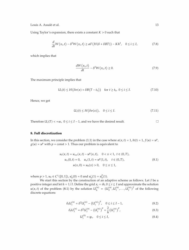
Using Taylor’s expansion, there exists a constant K > 0 such that
d
dtW
(xi, t
)− δ2W
(xi, t
)≥ αF
(H(δ + δBT)
)−Kh2, 0 ≤ i ≤ I, (7.8)
which implies that
dW(xi, t
)
dt− δ2W
(xi, t
)≥ 0. (7.9)
The maximum principle implies that
Ui(t) ≤ H(δv(x) + δB
(T − t0
))for t ≥ t0, 0 ≤ i ≤ I. (7.10)
Hence, we get
Ui(t) ≤ H(δv(x)
), 0 ≤ i ≤ I. (7.11)
Therefore Ui(T) < +∞, 0 ≤ i ≤ I − 1, and we have the desired result.
8. Full discretization
In this section, we consider the problem (1.1) in the case where a(x, t) = 1, b(t) = 1, f(u) = up,g(u) = up with p = const > 1. Thus our problem is equivalent to
ut(x, t) = uxx(x, t) − up(x, t), 0 < x < 1, t ∈ (0, T),
ux(0, t) = 0, ux(1, t) = up(1, t), t ∈ (0, T),
u(x, 0) = u0(x) > 0, 0 ≤ x ≤ 1,
(8.1)
where p > 1, u0 ∈ C1([0, 1]), u′0(0) = 0 and u′0(1) = up
0(1).We start this section by the construction of an adaptive scheme as follows. Let I be a
positive integer and let h = 1/I. Define the grid xi = ih, 0 ≤ i ≤ I and approximate the solutionu(x, t) of the problem (8.1) by the solution U
(n)h = (U(n)
0 , U(n)1 , . . . , U
(n)I )T of the following
discrete equations
δtU(n)i = δ2U
(n)i −
(U
(n)i
)p, 0 ≤ i ≤ I − 1, (8.2)
δtU(n)I = δ2U
(n)I −
(U
(n)I
)p+
2h
(U
(n)I
)p, (8.3)
U(0)i = ϕi, 0 ≤ i ≤ I, (8.4)
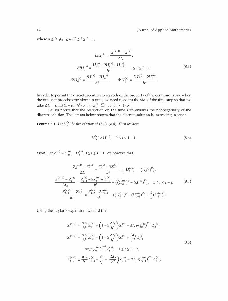
14 Journal of Applied Mathematics
where n ≥ 0, ϕi+1 ≥ ϕi, 0 ≤ i ≤ I − 1,
δtU(n)i =
U(n+1)i −U(n)
i
Δtn,
δ2U(n)i =
U(n)i+1 − 2U(n)
i +U(n)i−1
h2, 1 ≤ i ≤ I − 1,
δ2U(n)0 =
2U(n)1 − 2U(n)
0
h2, δ2U
(n)I =
2U(n)I−1 − 2U(n)
I
h2.
(8.5)
In order to permit the discrete solution to reproduce the property of the continuous one whenthe time t approaches the blow-up time, we need to adapt the size of the time step so that wetake Δtn = min{(1 − pτ)h2/3, τ/‖U(n)
h ‖p−1∞ }, 0 < τ < 1/p.
Let us notice that the restriction on the time step ensures the nonnegativity of thediscrete solution. The lemma below shows that the discrete solution is increasing in space.
Lemma 8.1. LetU(n)h
be the solution of (8.2)–(8.4). Then we have
U(n)i+1 ≥ U
(n)i , 0 ≤ i ≤ I − 1. (8.6)
Proof. Let Z(n)i = U(n)
i+1 −U(n)i , 0 ≤ i ≤ I − 1. We observe that
Z(n+1)0 − Z(n)
0
Δtn=Z
(n)1 − 3Z(n)
0
h2−((U
(n)1
)p −(U
(n)0
)p),
Z(n+1)i − Z(n)
i
Δtn=Z
(n)i+1 − 2Z(n)
i + Z(n)i−1
h2−((U
(n)i+1
)p −(U
(n)i
)p), 1 ≤ i ≤ I − 2,
Z(n+1)I−1 − Z(n)
I−1
Δtn=Z
(n)I−2 − 3Z(n)
I−1
h2−((U
(n)I
)p −(U
(n)I−1
)p)+
2h
(U
(n)I
)p.
(8.7)
Using the Taylor’s expansion, we find that
Z(n+1)0 =
Δtnh2
Z(n)1 +
(1 − 3
Δtnh2
)Z
(n)0 −Δtnp
(ξ(n)0
)p−1Z
(n)0 ,
Z(n+1)i =
Δtnh2
Z(n)i+1 +
(1 − 2
Δtnh2
)Z
(n)i +
Δtnh2
Z(n)i−1
−Δtnp(ξ(n)i
)p−1Z
(n)i , 1 ≤ i ≤ I − 2,
Z(n+1)I−1 ≥ Δtn
h2Z
(n)I−2 +
(1 − 3
Δtnh2
)Z
(n)I−1 −Δtnp
(ξ(n)I−1
)p−1Z
(n)I−1,
(8.8)
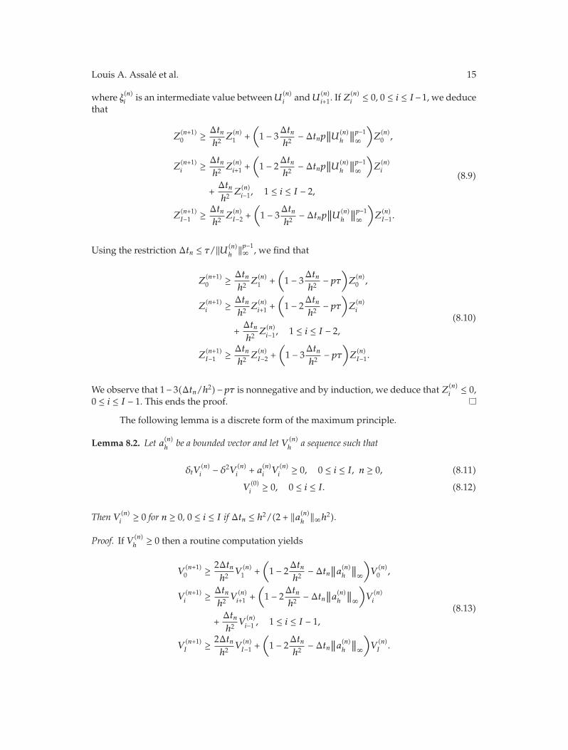
Louis A. Assale et al. 15
where ξ(n)i is an intermediate value between U(n)i and U(n)
i+1. If Z(n)i ≤ 0, 0 ≤ i ≤ I −1, we deduce
that
Z(n+1)0 ≥ Δtn
h2Z
(n)1 +
(1 − 3
Δtnh2−Δtnp
∥∥U(n)
h
∥∥p−1∞
)Z
(n)0 ,
Z(n+1)i ≥ Δtn
h2Z
(n)i+1 +
(1 − 2
Δtnh2−Δtnp
∥∥U(n)
h
∥∥p−1∞
)Z
(n)i
+Δtnh2
Z(n)i−1, 1 ≤ i ≤ I − 2,
Z(n+1)I−1 ≥ Δtn
h2Z
(n)I−2 +
(1 − 3
Δtnh2−Δtnp
∥∥U(n)
h
∥∥p−1∞
)Z
(n)I−1.
(8.9)
Using the restriction Δtn ≤ τ/‖U(n)h‖p−1∞ , we find that
Z(n+1)0 ≥ Δtn
h2Z
(n)1 +
(1 − 3
Δtnh2− pτ
)Z
(n)0 ,
Z(n+1)i ≥ Δtn
h2Z
(n)i+1 +
(1 − 2
Δtnh2− pτ
)Z
(n)i
+Δtnh2
Z(n)i−1, 1 ≤ i ≤ I − 2,
Z(n+1)I−1 ≥ Δtn
h2Z
(n)I−2 +
(1 − 3
Δtnh2− pτ
)Z
(n)I−1.
(8.10)
We observe that 1− 3(Δtn/h2)−pτ is nonnegative and by induction, we deduce that Z(n)i ≤ 0,
0 ≤ i ≤ I − 1. This ends the proof.
The following lemma is a discrete form of the maximum principle.
Lemma 8.2. Let a(n)h
be a bounded vector and let V (n)h
a sequence such that
δtV(n)i − δ2V
(n)i + a(n)i V
(n)i ≥ 0, 0 ≤ i ≤ I, n ≥ 0, (8.11)
V(0)i ≥ 0, 0 ≤ i ≤ I. (8.12)
Then V (n)i ≥ 0 for n ≥ 0, 0 ≤ i ≤ I if Δtn ≤ h2/(2 + ‖a(n)h ‖∞h
2).
Proof. If V (n)h≥ 0 then a routine computation yields
V(n+1)0 ≥ 2Δtn
h2V
(n)1 +
(1 − 2
Δtnh2−Δtn
∥∥a(n)h
∥∥∞
)V
(n)0 ,
V(n+1)i ≥ Δtn
h2V
(n)i+1 +
(1 − 2
Δtnh2−Δtn
∥∥a(n)h
∥∥∞
)V
(n)i
+Δtnh2
V(n)i−1 , 1 ≤ i ≤ I − 1,
V(n+1)I ≥ 2Δtn
h2V
(n)I−1 +
(1 − 2
Δtnh2−Δtn
∥∥a(n)h
∥∥∞
)V
(n)I .
(8.13)
16 Journal of Applied Mathematics
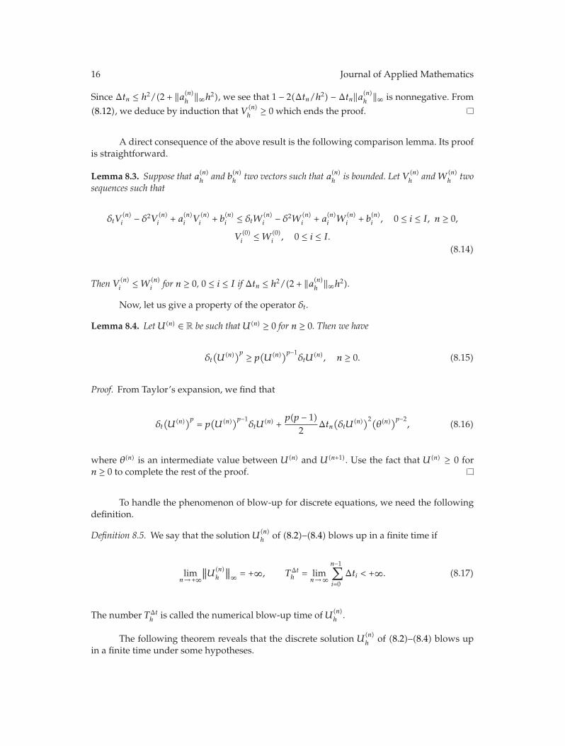
Since Δtn ≤ h2/(2 + ‖a(n)h ‖∞h2), we see that 1 − 2(Δtn/h2) −Δtn‖a(n)h ‖∞ is nonnegative. From
(8.12), we deduce by induction that V (n)h≥ 0 which ends the proof.
A direct consequence of the above result is the following comparison lemma. Its proofis straightforward.
Lemma 8.3. Suppose that a(n)h
and b(n)h
two vectors such that a(n)h
is bounded. Let V (n)h
andW (n)h
twosequences such that
δtV(n)i − δ2V
(n)i + a(n)i V
(n)i + b(n)i ≤ δtW (n)
i − δ2W(n)i + a(n)i W
(n)i + b(n)i , 0 ≤ i ≤ I, n ≥ 0,
V(0)i ≤W (0)
i , 0 ≤ i ≤ I.(8.14)
Then V (n)i ≤W (n)
i for n ≥ 0, 0 ≤ i ≤ I if Δtn ≤ h2/(2 + ‖a(n)h‖∞h2).
Now, let us give a property of the operator δt.
Lemma 8.4. LetU(n) ∈ R be such thatU(n) ≥ 0 for n ≥ 0. Then we have
δt(U(n))p ≥ p
(U(n))p−1
δtU(n), n ≥ 0. (8.15)
Proof. From Taylor’s expansion, we find that
δt(U(n))p = p
(U(n))p−1
δtU(n) +
p(p − 1)2
Δtn(δtU
(n))2(θ(n)
)p−2, (8.16)
where θ(n) is an intermediate value between U(n) and U(n+1). Use the fact that U(n) ≥ 0 forn ≥ 0 to complete the rest of the proof.
To handle the phenomenon of blow-up for discrete equations, we need the followingdefinition.
Definition 8.5. We say that the solution U(n)h of (8.2)–(8.4) blows up in a finite time if
limn→+∞
∥∥U(n)h
∥∥∞ = +∞, TΔt
h = limn→∞
n−1∑
i=0
Δti < +∞. (8.17)
The number TΔth is called the numerical blow-up time of U(n)
h .
The following theorem reveals that the discrete solution U(n)h of (8.2)–(8.4) blows up
in a finite time under some hypotheses.
Louis A. Assale et al. 17
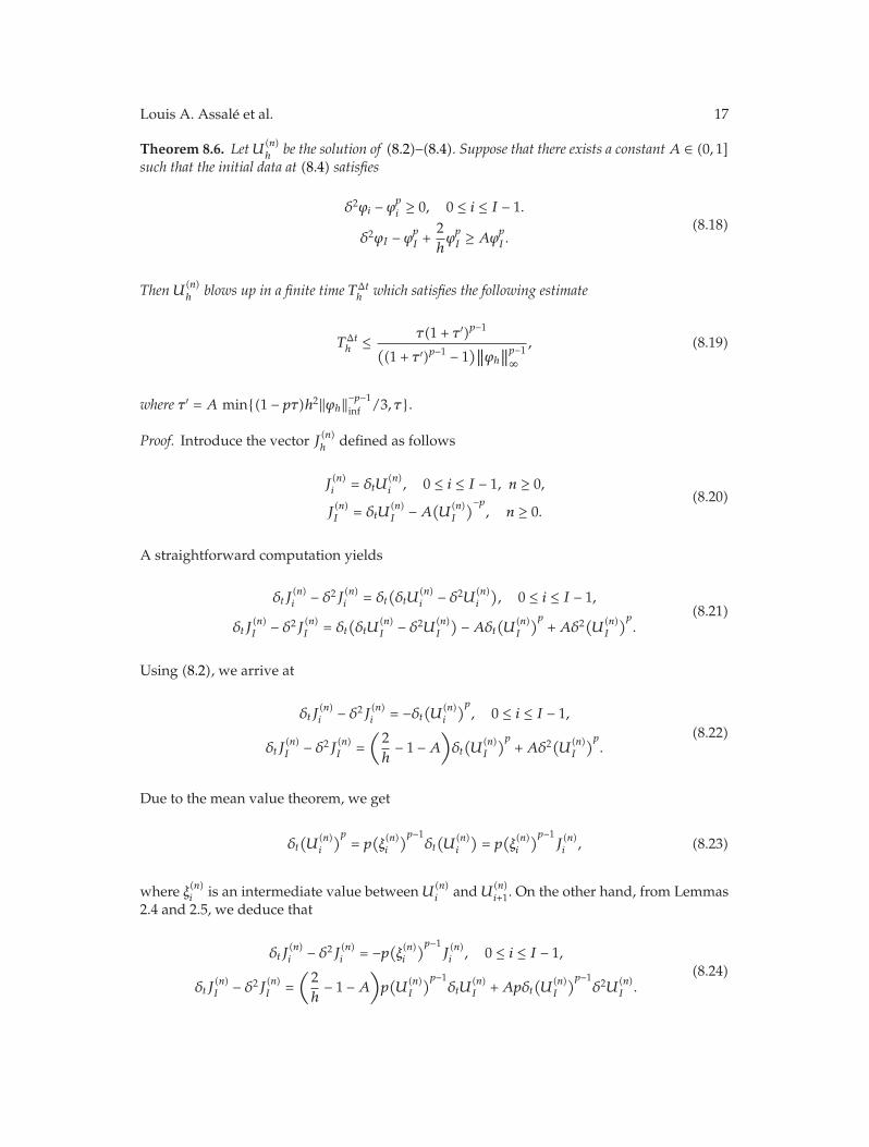
Theorem 8.6. LetU(n)h be the solution of (8.2)–(8.4). Suppose that there exists a constantA ∈ (0, 1]
such that the initial data at (8.4) satisfies
δ2ϕi − ϕp
i ≥ 0, 0 ≤ i ≤ I − 1.
δ2ϕI − ϕp
I +2hϕp
I ≥ Aϕp
I .(8.18)
ThenU(n)h
blows up in a finite time TΔth
which satisfies the following estimate
TΔth ≤
τ(1 + τ ′)p−1
((1 + τ ′)p−1 − 1
)∥∥ϕh∥∥p−1∞
, (8.19)
where τ ′ = A min{(1 − pτ)h2‖ϕh‖−p−1inf /3, τ}.
Proof. Introduce the vector J(n)h
defined as follows
J(n)i = δtU
(n)i , 0 ≤ i ≤ I − 1, n ≥ 0,
J(n)I = δtU
(n)I −A
(U
(n)I
)−p, n ≥ 0.
(8.20)
A straightforward computation yields
δtJ(n)i − δ2J
(n)i = δt
(δtU
(n)i − δ2U
(n)i
), 0 ≤ i ≤ I − 1,
δtJ(n)I − δ2J
(n)I = δt
(δtU
(n)I − δ2U
(n)I
)−Aδt
(U
(n)I
)p+Aδ2(U(n)
I
)p.
(8.21)
Using (8.2), we arrive at
δtJ(n)i − δ2J
(n)i = −δt
(U
(n)i
)p, 0 ≤ i ≤ I − 1,
δtJ(n)I − δ2J
(n)I =
(2h− 1 −A
)δt(U
(n)I
)p+Aδ2(U(n)
I
)p.
(8.22)
Due to the mean value theorem, we get
δt(U
(n)i
)p= p
(ξ(n)i
)p−1δt(U
(n)i
)= p
(ξ(n)i
)p−1J(n)i , (8.23)
where ξ(n)i is an intermediate value between U(n)i and U
(n)i+1. On the other hand, from Lemmas
2.4 and 2.5, we deduce that
δtJ(n)i − δ2J
(n)i = −p
(ξ(n)i
)p−1J(n)i , 0 ≤ i ≤ I − 1,
δtJ(n)I − δ2J
(n)I =
(2h− 1 −A
)p(U
(n)I
)p−1δtU
(n)I +Apδt
(U
(n)I
)p−1δ2U
(n)I .
(8.24)
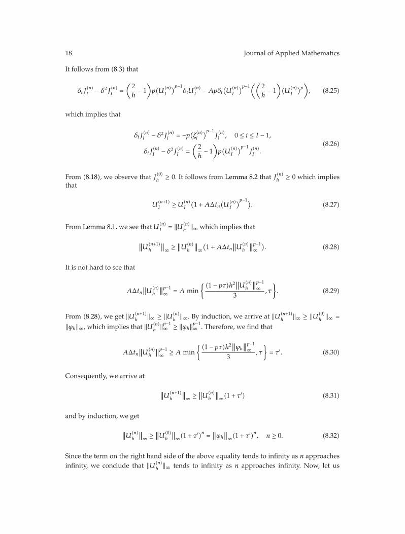
18 Journal of Applied Mathematics
It follows from (8.3) that
δtJ(n)I − δ2J
(n)I =
(2h− 1
)p(U
(n)I
)p−1δtU
(n)I −Apδt
(U
(n)I
)p−1((
2h− 1
)(U
(n)I
)p), (8.25)
which implies that
δtJ(n)i − δ2J
(n)i = −p
(ξ(n)i
)p−1J(n)i , 0 ≤ i ≤ I − 1,
δtJ(n)I − δ2J
(n)I =
(2h− 1
)p(U
(n)I
)p−1J(n)I .
(8.26)
From (8.18), we observe that J(0)h≥ 0. It follows from Lemma 8.2 that J(n)
h≥ 0 which implies
that
U(n+1)I ≥ U(n)
I
(1 +AΔtn
(U
(n)I
)p−1). (8.27)
From Lemma 8.1, we see that U(n)I = ‖U(n)
h‖∞ which implies that
∥∥U(n+1)h
∥∥∞ ≥
∥∥U(n)h
∥∥∞(1 +AΔtn
∥∥U(n)h
∥∥p−1∞
). (8.28)
It is not hard to see that
AΔtn∥∥U(n)
h
∥∥p−1∞ = A min
{(1 − pτ)h2∥∥U(n)
h
∥∥p−1∞
3, τ
}. (8.29)
From (8.28), we get ‖U(n+1)h‖∞ ≥ ‖U(n)
h‖∞. By induction, we arrive at ‖U(n+1)
h‖∞ ≥ ‖U(0)
h‖∞ =
‖ϕh‖∞, which implies that ‖U(n)h‖p−1∞ ≥ ‖ϕh‖
p−1∞ . Therefore, we find that
AΔtn∥∥U(n)
h
∥∥p−1∞ ≥ A min
{(1 − pτ)h2∥∥ϕh
∥∥p−1∞
3, τ
}= τ ′. (8.30)
Consequently, we arrive at
∥∥U(n+1)h
∥∥∞ ≥
∥∥U(n)h
∥∥∞(1 + τ ′) (8.31)
and by induction, we get
∥∥U(n)h
∥∥∞ ≥
∥∥U(0)h
∥∥∞(1 + τ ′)n =
∥∥ϕh∥∥∞(1 + τ ′)n, n ≥ 0. (8.32)
Since the term on the right hand side of the above equality tends to infinity as n approachesinfinity, we conclude that ‖U(n)
h‖∞ tends to infinity as n approaches infinity. Now, let us
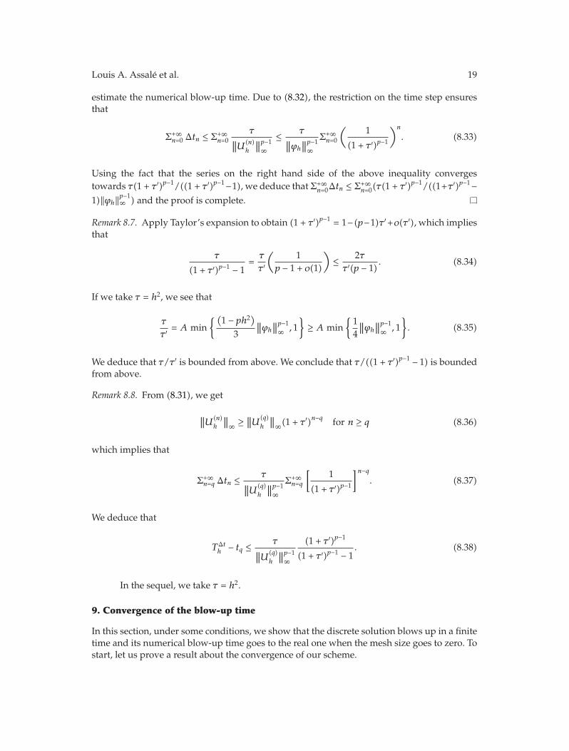
Louis A. Assale et al. 19
estimate the numerical blow-up time. Due to (8.32), the restriction on the time step ensuresthat
Σ+∞n=0 Δtn ≤ Σ+∞
n=0τ
∥∥U(n)
h
∥∥p−1∞
≤ τ∥∥ϕh
∥∥p−1∞
Σ+∞n=0
(1
(1 + τ ′)p−1
)n
. (8.33)
Using the fact that the series on the right hand side of the above inequality convergestowards τ(1 + τ ′)p−1/((1 + τ ′)p−1−1), we deduce that Σ+∞
n=0Δtn ≤ Σ+∞n=0(τ(1 + τ ′)p−1/((1+τ ′)p−1−
1)‖ϕh‖p−1∞ ) and the proof is complete.
Remark 8.7. Apply Taylor’s expansion to obtain (1 + τ ′)p−1 = 1−(p−1)τ ′+o(τ ′), which impliesthat
τ
(1 + τ ′)p−1 − 1=τ
τ ′
(1
p − 1 + o(1)
)≤ 2ττ ′(p − 1)
. (8.34)
If we take τ = h2, we see that
τ
τ ′= A min
{(1 − ph2)
3∥∥ϕh
∥∥p−1∞ , 1
}≥ A min
{14∥∥ϕh
∥∥p−1∞ , 1
}. (8.35)
We deduce that τ/τ ′ is bounded from above. We conclude that τ/((1 + τ ′)p−1 − 1) is boundedfrom above.
Remark 8.8. From (8.31), we get
∥∥U(n)h
∥∥∞ ≥
∥∥U(q)h
∥∥∞(1 + τ ′)n−q for n ≥ q (8.36)
which implies that
Σ+∞n=qΔtn ≤
τ∥∥U
(q)h
∥∥p−1∞
Σ+∞n=q
[1
(1 + τ ′)p−1
]n−q. (8.37)
We deduce that
TΔth − tq ≤
τ∥∥U
(q)h
∥∥p−1∞
(1 + τ ′)p−1
(1 + τ ′)p−1 − 1. (8.38)
In the sequel, we take τ = h2.
9. Convergence of the blow-up time
In this section, under some conditions, we show that the discrete solution blows up in a finitetime and its numerical blow-up time goes to the real one when the mesh size goes to zero. Tostart, let us prove a result about the convergence of our scheme.

20 Journal of Applied Mathematics
Theorem 9.1. Suppose that the problem (1.1) has a solution u ∈ C4,2([0, 1] × [0, T]). Assume thatthe initial data at (8.4) satisfies
∥∥ϕh − uh(0)
∥∥∞ = o(1) as h −→ 0. (9.1)
Then the problem (8.2)–(8.4) has a solution U(n)h
for h sufficiently small, 0 ≤ n ≤ J and we have thefollowing relation
max0≤n≤J
∥∥U(n)
h − uh(tn)∥∥∞ = O
(∥∥ϕh − uh(0)∥∥∞ + h2 + Δtn
)as h −→ 0, (9.2)
where J is such that∑J−1
n=0Δtn ≤ T and tn =∑n−1
j=0 Δtj .
Proof. For each h, the problem (8.2)–(8.4) has a solution U(n)h . Let N ≤ J be the greatest value
of n such that
∥∥U(n)h − uh(tn)
∥∥∞ < 1 for n < N. (9.3)
We know that N ≥ 1 because of (9.1). Due to the fact that u ∈ C4,2, there exists a positiveconstant K such that ‖u‖∞ ≤ K. Applying the triangle inequality, we have
∥∥U(n)h
∥∥∞ ≤
∥∥uh(tn)∥∥∞ +
∥∥U(n)h− uh
(tn)∥∥∞ ≤ 1 +K for n < N. (9.4)
Since u ∈ C4,2, using Taylor’s expansion, we find that
δtu(xi, tn
)− δ2u
(xi, tn
)= −up
(xi, tn
)+O
(h2) +O
(Δtn
), 0 ≤ i ≤ I − 1,
δtu(xI, tn
)− δ2u
(xI, tn
)= −up
(xI, tn
)+
2hup
(xI, tn
)+O
(h2) +O
(Δtn
).
(9.5)
Let e(n)h = U(n)h − uh(tn) be the error of discretization. From the mean value theorem, we get
δte(n)i − δ
2e(n)i = −p
(ξ(n)i
)p−1e(n)i +O
(h2) +O
(Δtn
), 0 ≤ i ≤ I − 1,
δte(n)I − δ
2e(n)I = p
(2h− 1
)(ξ(n)I
)p−1e(n)I +O
(h2) +O
(Δtn
),
(9.6)
where ξ(n)i is an intermediate value between u(xi, tn) and U
(n)i . Hence, there exist positive
constants L and K such that
δte(n)i − δ
2e(n)i ≤ −p
(ξ(n)i
)p−1e(n)i + Lh2 + LΔtn, 0 ≤ i ≤ I − 1, n < N,
δte(n)I − δ
2e(n)I ≤ p
(2h− 1
)(ξ(n)I
)p−1e(n)I + Lh2 + LΔtn, n < N.
(9.7)
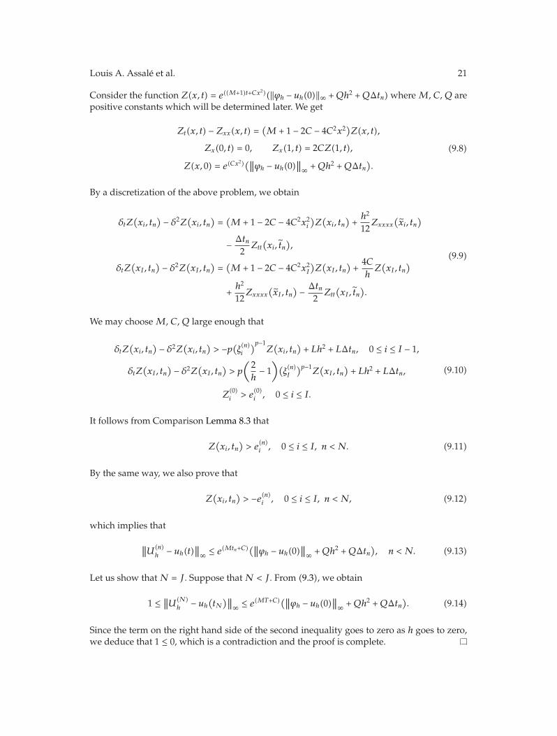
Louis A. Assale et al. 21
Consider the function Z(x, t) = e((M+1)t+Cx2)(‖ϕh − uh(0)‖∞ +Qh2 +QΔtn) where M, C, Q arepositive constants which will be determined later. We get
Zt(x, t) − Zxx(x, t) =(M + 1 − 2C − 4C2x2)Z(x, t),
Zx(0, t) = 0, Zx(1, t) = 2CZ(1, t),
Z(x, 0) = e(Cx2)(∥∥ϕh − uh(0)
∥∥∞ +Qh2 +QΔtn
).
(9.8)
By a discretization of the above problem, we obtain
δtZ(xi, tn
)− δ2Z
(xi, tn
)=(M + 1 − 2C − 4C2x2
i
)Z(xi, tn
)+h2
12Zxxxx
(xi, tn
)
− Δtn2Ztt
(xi, tn
),
δtZ(xI, tn
)− δ2Z
(xI, tn
)=(M + 1 − 2C − 4C2x2
I
)Z(xI, tn
)+
4ChZ(xI, tn
)
+h2
12Zxxxx
(xI , tn
)− Δtn
2Ztt
(xI, tn
).
(9.9)
We may choose M, C, Q large enough that
δtZ(xi, tn
)− δ2Z
(xi, tn
)> −p
(ξ(n)i
)p−1Z(xi, tn
)+ Lh2 + LΔtn, 0 ≤ i ≤ I − 1,
δtZ(xI, tn
)− δ2Z
(xI, tn
)> p
(2h− 1
)(ξ(n)I
)p−1Z(xI, tn
)+ Lh2 + LΔtn,
Z(0)i > e
(0)i , 0 ≤ i ≤ I.
(9.10)
It follows from Comparison Lemma 8.3 that
Z(xi, tn
)> e
(n)i , 0 ≤ i ≤ I, n < N. (9.11)
By the same way, we also prove that
Z(xi, tn
)> −e(n)i , 0 ≤ i ≤ I, n < N, (9.12)
which implies that
∥∥U(n)h − uh(t)
∥∥∞ ≤ e
(Mtn+C)(∥∥ϕh − uh(0)
∥∥∞ +Qh2 +QΔtn
), n < N. (9.13)
Let us show that N = J . Suppose that N < J . From (9.3), we obtain
1 ≤∥∥U(N)
h− uh
(tN
)∥∥∞ ≤ e
(MT+C)(∥∥ϕh − uh(0)∥∥∞ +Qh2 +QΔtn
). (9.14)
Since the term on the right hand side of the second inequality goes to zero as h goes to zero,we deduce that 1 ≤ 0, which is a contradiction and the proof is complete.
22 Journal of Applied Mathematics
Now, we are in a position to state the main theorem of this section.
Theorem 9.2. Suppose that the problem (1.1) has a solution u which blows up in a finite time T0 andu ∈ C4,2([0, 1] × [0, T0)). Assume that the initial data at (2.3) satisfies
∥∥ϕh − uh(0)
∥∥∞ = o(1) as h −→ 0. (9.15)
Under the assumption of Theorem 8.6, the problem (8.2)–(8.4) has a solutionU(n)h
which blows up ina finite time TΔt
h and the following relation holds
limh→ 0
TΔth = T0. (9.16)
Proof. We know from Remark 8.7 that τ(1 + τ ′)/((1 + τ ′)p−1 − 1) is bounded. Letting ε > 0,there exists a constant R > 0 such that
τ(1 + τ ′)p−1
xp−1((1 + τ ′)p−1 − 1
) <ε
2for x ∈ [R,∞). (9.17)
Since u blows up at the time T0, there exists T1 ∈ (T0 − ε/2, T0) such that ‖u(·, t)‖∞ ≥ 2R fort ∈ [T1, T0). Let T2 = (T1+T0)/2 and let q be a positive integer such that tq =
∑q−1n=0Δtn ∈ [T1, T2]
for h small enough. We have 0 < ‖uh(tn)‖∞ < ∞ for n ≤ q. It follows from Theorem 4.3 thatthe problem (2.1)–(2.3) has a solution U(n)
hwhich obeys ‖U(n)
h−uh(tn)‖∞ < R for n ≤ q, which
implies that
∥∥U(q)h
∥∥∞ ≥
∥∥uh(tq)∥∥∞ −
∥∥U(q)h − uh
(tq)∥∥∞ ≥ R. (9.18)
From Theorem 8.6, U(n)h blows up at the time TΔt
h . It follows from Remark 8.8 and (9.17) that
|TΔth− tq| ≤ τ(1 + τ ′)p−1‖U(q)
h‖1−p∞ /((1 + τ ′)p−1 − 1) < ε/2 because ‖U(q)
h‖∞ ≥ R. We deduce that
|T0 − TΔth| ≤ |T0 − tq| + |tq − TΔt
h| ≤ ε/2 + ε/2 ≤ ε, which leads us to the result.
10. Numerical experiments
In this section, we present some numerical approximations to the blow-up time of (1.1) in thecase where a(x, t) = λ > 0, f(u) = up, g(u) = uq, b(t) = 1 with p = const > 1, q = const > 1. Weapproximate the solution u of (1.1) by the solution U(n)
h of the following explicit scheme
δtU(n)i = δ2U
(n)i − λ
(U
(n)i
)p−1U
(n+1)i , 0 ≤ i ≤ I − 1,
δtU(n)I = δ2U
(n)I +
2h
(U
(n)I
)q− λ
(U
(n)I
)p−1U
(n+1)I ,
U(0)i = ϕi ≥ 0, 0 ≤ i ≤ I,
(10.1)
Louis A. Assale et al. 23
We also approximate the solution u of (1.1) by the solution U(n)h of the implicit scheme below
δtU(n)i = δ2U
(n+1)i − λ
(U
(n)i
)p−1U
(n+1)i , 0 ≤ i ≤ I − 1,
δtU(n)I = δ2U
(n+1)I +
2h
(U
(n)I
)q− λ
(U
(n)I
)p−1U
(n+1)I ,
U(0)i = ϕi ≥ 0, 0 ≤ i ≤ I.
(10.2)
For the time step, we take n ≥ 0, Δtn = min(h2/2, τ‖U(n)h ‖
1−p∞ ) for the explicit scheme and
Δtn = τ‖U(n)h‖1−p∞ for the implicit scheme.
The problem described in (10.1) may be rewritten as follows
U(n+1)0 =
2(Δtn/h2)U(n)
1 +(1 − 2
(Δtn/h2))U(n)
0
1 + λΔtn(U
(n)0
)p−1,
U(n+1)i =
2(Δtn/h2)U(n)
i+1 +(1 − 2
(Δtn/h2))U(n)
i + 2(Δtn/h2)U(n)
i−1
1 + λΔtn(U
(n)i
)p−1,
U(n+1)I =
2(Δtn/h2)U(n)
I−1 +(1 − 2
(Δtn/h2))U(n)
I + 2(Δtn/h2)(U(n)
I
)q
1 + λΔtn(U
(n)I
)p−1.
(10.3)
Let us notice that the restriction on the time step Δtn ≤ h2/2 ensures the nonnegativity of thediscrete solution.
The implicit scheme may be rewritten in the following form
AnhU
(n+1)h
= Fn, (10.4)
where
A(n)h
=
⎛
⎜⎜⎜⎜⎜⎜⎜⎝
a0 b0 0 · · · 0c1 a1 b1 0 · · ·
0. . . . . . . . .
.... . . . . . . . . bI−1
0 · · · 0 cI aI
⎞
⎟⎟⎟⎟⎟⎟⎟⎠
,
ai = 1 + 2Δtnh2
+ λΔtn(U
(n)i
)p−1, 0 ≤ i ≤ I,
bi = −2Δtnh2
, i = 0, . . . , I − 1,
ci = −2Δtnh2
, i = 1, . . . , I,
(Fn)i = U(n)i , i = 0, . . . , I − 1,
(Fn)I = U(n)I +
2hΔtn
(U
(n)I
)q.
(10.5)
24 Journal of Applied Mathematics
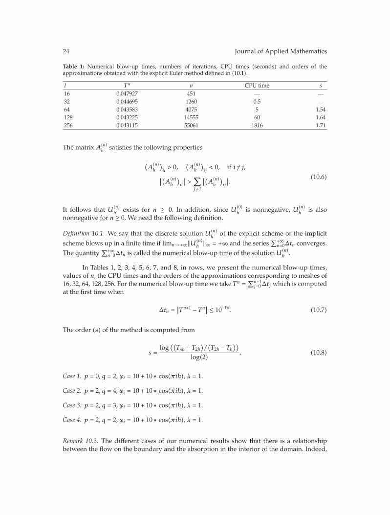
Table 1: Numerical blow-up times, numbers of iterations, CPU times (seconds) and orders of theapproximations obtained with the explicit Euler method defined in (10.1).
I Tn n CPU time s16 0.047927 451 — —32 0.044695 1260 0.5 —64 0.043583 4075 5 1.54128 0.043225 14555 60 1.64256 0.043115 55061 1816 1.71
The matrix A(n)h satisfies the following properties
(A
(n)h
)ii> 0,
(A
(n)h
)ij< 0, if i /= j,
∣∣(A(n)h
)ii
∣∣ >∑
j /= i
∣∣(A(n)h
)ij
∣∣.(10.6)
It follows that U(n)h exists for n ≥ 0. In addition, since U
(0)h is nonnegative, U(n)
h is alsononnegative for n ≥ 0. We need the following definition.
Definition 10.1. We say that the discrete solution U(n)h
of the explicit scheme or the implicitscheme blows up in a finite time if limn→+∞‖U(n)
h‖∞ = +∞ and the series
∑+∞n=0Δtn converges.
The quantity∑+∞
n=0Δtn is called the numerical blow-up time of the solution U(n)h .
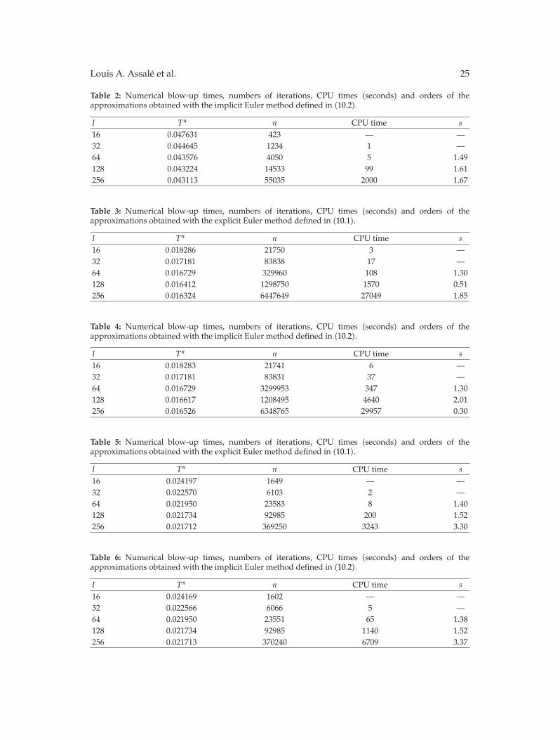
In Tables 1, 2, 3, 4, 5, 6, 7, and 8, in rows, we present the numerical blow-up times,values of n, the CPU times and the orders of the approximations corresponding to meshes of16, 32, 64, 128, 256. For the numerical blow-up time we take Tn =
∑n−1j=0 Δtj which is computed
at the first time when
Δtn =∣∣Tn+1 − Tn
∣∣ ≤ 10−16. (10.7)
The order (s) of the method is computed from
s =log
((T4h − T2h
)/(T2h − Th
))
log(2). (10.8)
Case 1. p = 0, q = 2, ϕi = 10 + 10 ∗ cos(πih), λ = 1.
Case 2. p = 2, q = 4, ϕi = 10 + 10 ∗ cos(πih), λ = 1.
Case 3. p = 2, q = 3, ϕi = 10 + 10 ∗ cos(πih), λ = 1.
Case 4. p = 2, q = 2, ϕi = 10 + 10 ∗ cos(πih), λ = 1.
Remark 10.2. The different cases of our numerical results show that there is a relationshipbetween the flow on the boundary and the absorption in the interior of the domain. Indeed,
Louis A. Assale et al. 25
Table 2: Numerical blow-up times, numbers of iterations, CPU times (seconds) and orders of theapproximations obtained with the implicit Euler method defined in (10.2).
I Tn n CPU time s16 0.047631 423 — —32 0.044645 1234 1 —64 0.043576 4050 5 1.49128 0.043224 14533 99 1.61256 0.043113 55035 2000 1.67
Table 3: Numerical blow-up times, numbers of iterations, CPU times (seconds) and orders of theapproximations obtained with the explicit Euler method defined in (10.1).
I Tn n CPU time s16 0.018286 21750 3 —32 0.017181 83838 17 —64 0.016729 329960 108 1.30128 0.016412 1298750 1570 0.51256 0.016324 6447649 27049 1.85
Table 4: Numerical blow-up times, numbers of iterations, CPU times (seconds) and orders of theapproximations obtained with the implicit Euler method defined in (10.2).
I Tn n CPU time s16 0.018283 21741 6 —32 0.017181 83831 37 —64 0.016729 3299953 347 1.30128 0.016617 1208495 4640 2.01256 0.016526 6348765 29957 0.30
Table 5: Numerical blow-up times, numbers of iterations, CPU times (seconds) and orders of theapproximations obtained with the explicit Euler method defined in (10.1).
I Tn n CPU time s16 0.024197 1649 — —32 0.022570 6103 2 —64 0.021950 23583 8 1.40128 0.021734 92985 200 1.52256 0.021712 369250 3243 3.30
Table 6: Numerical blow-up times, numbers of iterations, CPU times (seconds) and orders of theapproximations obtained with the implicit Euler method defined in (10.2).
I Tn n CPU time s16 0.024169 1602 — —32 0.022566 6066 5 —64 0.021950 23551 65 1.38128 0.021734 92985 1140 1.52256 0.021713 370240 6709 3.37
26 Journal of Applied Mathematics
U(i,n
)
0
0.5
1
1.5
2×10¹³
i
2015
105
0n
0100
200300
400500
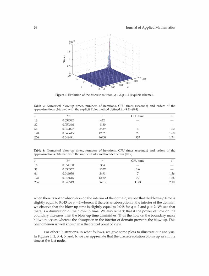
Figure 1: Evolution of the discrete solution, q = 2, p = 2 (explicit scheme).
Table 7: Numerical blow-up times, numbers of iterations, CPU times (seconds) and orders of theapproximations obtained with the explicit Euler method defined in (8.2)–(8.4).
I Tn n CPU time s16 0.054342 422 — —32 0.050346 1130 — —64 0.049027 3539 4 1.60128 0.048615 12020 28 1.68256 0.048491 46439 937 1.74
Table 8: Numerical blow-up times, numbers of iterations, CPU times (seconds) and orders of theapproximations obtained with the implicit Euler method defined in (10.2).
I Tn n CPU time s16 0.054158 364 — —32 0.050332 1077 0.6 —64 0.049030 3491 7 1.56128 0.048616 12358 79 1.66256 0.048519 36919 1123 2.10
when there is not an absorption on the interior of the domain, we see that the blow-up time isslightly equal to 0.043 for q = 2 whereas if there is an absorption in the interior of the domain,we observe that the blow-up time is slightly equal to 0.048 for q = 2 and p = 2. We see thatthere is a diminution of the blow-up time. We also remark that if the power of flow on theboundary increases then the blow-up time diminishes. Thus the flow on the boundary makeblow-up occurs whereas the absorption in the interior of domain prevents the blow-up. Thisphenomenon is well known in a theoretical point of view.
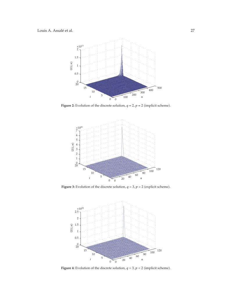
For other illustrations, in what follows, we give some plots to illustrate our analysis.In Figures 1, 2, 3, 4, 5, and, 6, we can appreciate that the discrete solution blows up in a finitetime at the last node.
Louis A. Assale et al. 27
U(i,n
)
0
0.5
1
1.5
2×10¹³
i
2015
105
0n
0100
200300
400500
Figure 2: Evolution of the discrete solution, q = 2, p = 2 (implicit scheme).
U(i,n
)
0
1
2
3
4
5
6
7×10²¹
i
2015
105
0n
020
4060
80100
120
Figure 3: Evolution of the discrete solution, q = 3, p = 2 (explicit scheme).
U(i,n
)
0
0.5
1
1.5
2
2.5×1024
i
2015
105
0n
020
4060
80100
120
Figure 4: Evolution of the discrete solution, q = 3, p = 2 (implicit scheme).

28 Journal of Applied Mathematics
U(i,n
)
0
1
2
3
4
5
6×10¹⁵
i
2015
105
0n
020
4060
80100
Figure 5: Evolution of the discrete solution, q = 4, p = 2 (explicit scheme).
U(i,n
)
0
0.5
1
1.5
2
2.5×1033
i
2015
105
0n
020
4060
80100
Figure 6: Evolution of the discrete solution, q = 4, p = 2 (implicit scheme).
Acknowledgments
We want to thank the anonymous referee for the throughout reading of the manuscript andseveral suggestions that help us to improve the presentation of the paper.
References
[1] T. K. Boni, “Sur l’explosion et le comportement asymptotique de la solution d’une equationparabolique semi-lineaire du second ordre,” Comptes Rendus de l’Academie des Sciences. Serie I, vol.326, no. 3, pp. 317–322, 1998.
[2] T. K. Boni, “On blow-up and asymptotic behavior of solutions to a nonlinear parabolic equationof second order with nonlinear boundary conditions,” Commentationes Mathematicae UniversitatisCarolinae, vol. 40, no. 3, pp. 457–475, 1999.
[3] M. Chipot, M. Fila, and P. Quittner, “Stationary solutions, blow up and convergence to stationarysolutions for semilinear parabolic equations with nonlinear boundary conditions,” Acta MathematicaUniversitatis Comenianae, vol. 60, no. 1, pp. 35–103, 1991.
[4] V. A. Galaktionov and J. L. Vazquez, “The problem of blow-up in nonlinear parabolic equations,”Discrete and Continuous Dynamical Systems. Series A, vol. 8, no. 2, pp. 399–433, 2002.

Louis A. Assale et al. 29
[5] P. Quittner and P. Souplet, Superlinear Parabolic Problems: Blow-up, Global Existence and Steady States,Birkhauser Advanced Texts. Basler Lehrbucher, Birkhauser, Basel, Switzerland, 2007.
[6] A. A. Samarskii, V. A. Galaktionov, S. P. Kurdyumov, and A. P. Mikhailov, Blow-up in Problems forQuasilinear Parabolic Equations, Nauka, Moscow, Russia, 1987.
[7] A. A. Samarskii, V. A. Galaktionov, S. P. Kurdyumov, and A. P. Mikhailov, Blow-up in Problems forQuasilinear Parabolic Equations, Walter de Gruyter, Berlin, Germany, 1995.
[8] L. M. Abia, J. C. Lopez-Marcos, and J. Martınez, “On the blow-up time convergence ofsemidiscretizations of reaction-diffusion equations,” Applied Numerical Mathematics, vol. 26, no. 4, pp.399–414, 1998.
[9] T. Nakagawa, “Blowing up of a finite difference solution to ut = uxx + u2,” Applied Mathematics andOptimization, vol. 2, no. 4, pp. 337–350, 1975.
[10] T. K. Boni, “Extinction for discretizations of some semilinear parabolic equations,” Comptes Rendus del’Academie des Sciences. Serie I, vol. 333, no. 8, pp. 795–800, 2001.
[11] G. Acosta, J. Fernandez Bonder, P. Groisman, and J. D. Rossi, “Simultaneous vs. non-simultaneousblow-up in numerical approximations of a parabolic system with non-linear boundary conditions,”M2AN, vol. 36, no. 1, pp. 55–68, 2002.
[12] G. Acosta, J. Fernandez Bonder, P. Groisman, and J. D. Rossi, “Numerical approximation of a parabolicproblem with a nonlinear boundary condition in several space dimensions,” Discrete and ContinuousDynamical Systems. Series B, vol. 2, no. 2, pp. 279–294, 2002.
[13] C. Brandle, P. Groisman, and J. D. Rossi, “Fully discrete adaptive methods for a blow-up problem,”Mathematical Models & Methods in Applied Sciences, vol. 14, no. 10, pp. 1425–1450, 2004.
[14] C. Brandle, F. Quiros, and J. D. Rossi, “An adaptive numerical method to handle blow-up in aparabolic system,” Numerische Mathematik, vol. 102, no. 1, pp. 39–59, 2005.
[15] R. G. Duran, J. I. Etcheverry, and J. D. Rossi, “Numerical approximation of a parabolic problem with anonlinear boundary condition,” Discrete and Continuous Dynamical Systems, vol. 4, no. 3, pp. 497–506,1998.
[16] J. Fernandez Bonder and J. D. Rossi, “Blow-up vs. spurious steady solutions,” Proceedings of theAmerican Mathematical Society, vol. 129, no. 1, pp. 139–144, 2001.
[17] A. de Pablo, M. Perez-Llanos, and R. Ferreira, “Numerical blow-up for the p-Laplacian equationwith a nonlinear source,” in Proceedings of the 11th International Conference on Differential Equations(Equadiff ’05), pp. 363–367, Bratislava, Slovakia, July 2005.
[18] M. N. Le Roux, “Semidiscretization in time of nonlinear parabolic equations with blowup of thesolution,” SIAM Journal on Numerical Analysis, vol. 31, no. 1, pp. 170–195, 1994.
[19] M. N. Le Roux, “Semi-discretization in time of a fast diffusion equation,” Journal of MathematicalAnalysis and Applications, vol. 137, no. 2, pp. 354–370, 1989.
[20] D. Nabongo and T. K. Boni, “Numerical blow-up and asymptotic behavior for a semilinear parabolicequation with a nonlilnear boundary condition,” Albanian Journal of Mathematics, vol. 2, no. 2, pp.111–124, 2008.
[21] D. Nabongo and T. K. Boni, “Numerical blow-up solutions of localized semilinear parabolicequations,” Applied Mathematical Sciences, vol. 2, no. 21–24, pp. 1145–1160, 2008.
[22] F. K. N’gohisse and T. K. Boni, “Numerical blow-up solution for some semilinear heat equation,”Electronic Transactions on Numerical Analysis, vol. 30, pp. 247–257, 2008.

Submit your manuscripts athttp://www.hindawi.com
Hindawi Publishing Corporationhttp://www.hindawi.com Volume 2014
MathematicsJournal of
Hindawi Publishing Corporationhttp://www.hindawi.com Volume 2014
Mathematical Problems in Engineering
Hindawi Publishing Corporationhttp://www.hindawi.com
Differential EquationsInternational Journal of
Volume 2014
Applied MathematicsJournal of
Hindawi Publishing Corporationhttp://www.hindawi.com Volume 2014
Probability and StatisticsHindawi Publishing Corporationhttp://www.hindawi.com Volume 2014
Journal of
Hindawi Publishing Corporationhttp://www.hindawi.com Volume 2014
Mathematical PhysicsAdvances in
Complex AnalysisJournal of
Hindawi Publishing Corporationhttp://www.hindawi.com Volume 2014
OptimizationJournal of
Hindawi Publishing Corporationhttp://www.hindawi.com Volume 2014
CombinatoricsHindawi Publishing Corporationhttp://www.hindawi.com Volume 2014
International Journal of
Hindawi Publishing Corporationhttp://www.hindawi.com Volume 2014
Operations ResearchAdvances in
Journal of
Hindawi Publishing Corporationhttp://www.hindawi.com Volume 2014
Function Spaces
Abstract and Applied AnalysisHindawi Publishing Corporationhttp://www.hindawi.com Volume 2014
International Journal of Mathematics and Mathematical Sciences
Hindawi Publishing Corporationhttp://www.hindawi.com Volume 2014
The Scientific World JournalHindawi Publishing Corporation http://www.hindawi.com Volume 2014
Hindawi Publishing Corporationhttp://www.hindawi.com Volume 2014
Algebra
Discrete Dynamics in Nature and Society
Hindawi Publishing Corporationhttp://www.hindawi.com Volume 2014
Hindawi Publishing Corporationhttp://www.hindawi.com Volume 2014
Decision SciencesAdvances in
Discrete MathematicsJournal of
Hindawi Publishing Corporationhttp://www.hindawi.com
Volume 2014 Hindawi Publishing Corporationhttp://www.hindawi.com Volume 2014
Stochastic AnalysisInternational Journal of