arX

iv:m

ath/

0702

247v

1 [

mat

h.A

P] 9

Feb

200

7 BOUNDARY SINGULARITIES FOR WEAK SOLUTIONS OF SEMILINEAR

ELLIPTIC PROBLEMS

MANUEL DEL PINO, MONICA MUSSO, FRANK PACARD

Abstract. Let Ω be a bounded domain in RN , N ≥ 2, with smooth boundary ∂Ω. We

construct positive weak solutions of the problem ∆u + up = 0 in Ω, which vanish in suitabletrace sense on ∂Ω, but which are singular at prescribed single points if p is equal or slightlyabove N+1

N−1. Similar constructions are carried out for solutions which are singular on any given

embedded submanifold of ∂Ω of dimension 0 ≤ k ≤ N − 2, if p equals or it is slightly aboveN−k+1

N−k−1, and even on countable families of these objects, dense on a given closed set. The

role of this exponent, first discovered by Brezis and Turner [1] for boundary regularity when

p < N+1

N−1, parallels that of p = N

N−2for interior singularities.

1. Introduction and statement of main results

Let Ω be a bounded domain in RN , with smooth boundary ∂Ω. A model of nonlinear elliptic

boundary value problem is the classical Lane-Emden-Fowler equation,

∆u+ up = 0 in Ω

u > 0 in Ω

u = 0 on ∂Ω

(1.1)

where p > 1. We are interested in finding solutions to this problem which are smooth in Ω andequal to 0 almost everywhere on ∂Ω with respect to surface measure. More precisely, we wantto study solutions to problem (1.1) that satisfy the boundary condition in a suitable trace sense,while not necessarily in a continuous fashion.

Following Brezis & Turner [1] and Quittner & Souplet [11], we say that a positive functionu ∈ C∞(Ω) is a very weak solution of problem (1.1) if

u, updist (x, ∂Ω) ∈ L1(Ω)

and∫

Ω

(u∆v + up v) dx = 0 for all v ∈ C2(Ω) with v = 0 on ∂Ω.

From the results in [1, 11], it follows that if p satisfies the constraint

1 < p <N + 1

N − 1(1.2)

1

2 MANUEL DEL PINO, MONICA MUSSO, FRANK PACARD

then a very weak solution u is actually in H10 (Ω), and it is a weak solution in the usual variational

sense:

u ∈ H10 (Ω),

∫

Ω

(∇u∇v − up v) dx = 0 for all v ∈ H10 (Ω).

Elliptic regularity then yields u ∈ C2(Ω), so that u solves (1.1) classically. As it is well-known, aconstrained minimization procedure involving Sobolev’s embedding implies existence of a weak-variational solution to (1.1) for 1 < p < N+2

N−2 . A natural question is then whether very weak

solutions of (1.1) are classical within a broader range of exponents than (1.2). Partially answeringthis question negatively, Souplet [12] constructed an example of a positive function a ∈ L∞(Ω)such that Problem (1.1), with up replaced by a(x)up for p > N+1

N−1 , has a very weak solution whichis unbounded, developing a point singularity on the boundary.

The exponent p = N+1N−1 is thus critical in what concerns to boundary regularity for very

weak solutions. The aim of this paper is to construct solutions to Problem (1.1) with prescribedsingularities on the boundary. To state an important special case of our main results we need adefinition:

Definition 1.1. Let u(x) be a function defined in Ω and x0 ∈ ∂Ω. We say that

u(x) → ℓ as x→ x0 non-tangentially

if

limΓα(x0)∋x→x0

u(x) = ℓ for all α ∈ [0,π

2),

where Γα(x0) denotes the cone with vertex ξi, and angle α with respect to its axis, the innernormal to ∂Ω at x0.

We have the validity of the following result.

Theorem 1.1. There exists a number pN > N+1N−1 such that if p satisfies

N + 1

N − 1≤ p < pN ,

then the following holds: given points ξ1, ξ2, . . . , ξk ∈ ∂Ω, there exists a very weak solution u toproblem (1.1) such that u ∈ C2(Ω \ ξ1, . . . , ξk) and

u(x) → +∞ as x→ ξi non-tangentially, for all i = 1, . . . , k.

The study of the behavior near an isolated boundary singularity of any positive solution of(1.1) when when the exponent p ≥ N+1

N−1 was recently achieved by Bidaut-Veron-Ponce-Veron in

[3].

BOUNDARY SINGULARITIES FOR WEAK SOLUTIONS 3

1.1. The parallel with p = NN−2 and interior singularities. The role of the exponent p =

N+1N−1 parallels that of p = N

N−2 for solutions to problem (1.1) with interior singularities. Let us

recall that if u ∈ Lp(Ω) is a positive distributional solution of (1.1) and 1 < p < NN−2 , then u is

smooth in Ω. On the other hand, for p ≥ NN−2 , distributional solutions of (1.1) with prescribed

interior singularities are built in [7, 9, 10, 4, 8, 5, 6]. Basic cells in those constructions are radiallysymmetric singular solutions u = u(|x|) for the equation

∆u+ up = 0. (1.3)

Whenever p > NN−2 , the function

u0(|x|) = cp,N |x|−2

p−1 , cp,N =

[

2

p− 1(N − 2 −

2

p− 1)

]1

p−1

, (1.4)

is a explicit singular solution of (1.3) in RN \ 0. If, in addition, N

N−2 < p < N+2N−2 , phase plane

analysis for the ODE corresponding to radial solutions of (1.3), yields existence of a singularpositive solution u1 which connects the behavior of u0 near the origin with fast decay at infinity,

u1(|x|) = cp,N |x|−2

p−1 (1 + o(1)) as x→ 0, (1.5)

u1(|x|) = |x|−(N−2)(1 + o(1)) as |x| → +∞, (1.6)

(note that N − 2 > 2p−1 ). The scalings uλ(r) = λ

2p−1 u1(λr) with λ > 0 are then solutions of

(1.3) that have the same behavior near the origin but which become very small as λ → 0+ onany compact subset of R

N \ 0. Thus, given points

ξ1, ξ2, . . . , ξk ∈ Ω,

the function

u∗(x) =

k∑

i=1

uλ(|x− ξi|)

constitutes a “good approximation” for small λ > 0 to a singular solution of Problem (1.1).Linear theory and perturbation arguments lead to establish the presence of an actual solution to(1.1) near u∗, see [8]. When p = N

N−2 a similar construction can be carried out, see [10]. Basic

cell u1 corresponds in this case to a positive radial solution u1 of equation (1.3) in B(0, 1) with

u1(|x|) = cN |x|−(N−2) log(1/|x|)−N−2

2 (1 + o(1)) as x→ 0. (1.7)

In this case the scalings uλ(x) = λN−2

2 u1(λx) have the same behavior as u1 at the origin, andthey approach zero as λ→ 0+, uniformly on compact subsets of R

N \ 0.

1.2. The basic cells: singular solutions on a half-space. In the construction of the solutionspredicted by Theorem 1.1 we will follow a scheme similar to that described above for interiorsingularities. Basic cells will now be positive solutions of equation (1.3) defined on the half-space,

RN+ := x = (x1, . . . , xN ) / xN > 0

4 MANUEL DEL PINO, MONICA MUSSO, FRANK PACARD

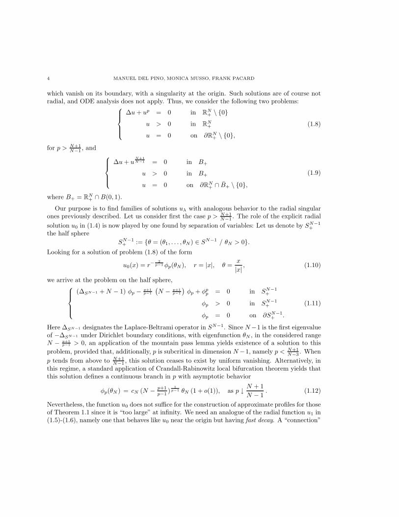
which vanish on its boundary, with a singularity at the origin. Such solutions are of course notradial, and ODE analysis does not apply. Thus, we consider the following two problems:

∆u+ up = 0 in RN+ \ 0

u > 0 in RN+

u = 0 on ∂RN+ \ 0,

(1.8)

for p > N+1N−1 , and

∆u+ uN+1

N−1 = 0 in B+

u > 0 in B+

u = 0 on ∂RN+ ∩ B+ \ 0,

(1.9)

where B+ = RN+ ∩B(0, 1).

Our purpose is to find families of solutions uλ with analogous behavior to the radial singularones previously described. Let us consider first the case p > N+1

N−1 . The role of the explicit radial

solution u0 in (1.4) is now played by one found by separation of variables: Let us denote by SN−1+

the half sphere

SN−1+ := θ = (θ1, . . . , θN) ∈ SN−1 / θN > 0.

Looking for a solution of problem (1.8) of the form

u0(x) = r−2

p−1φp(θN ), r = |x|, θ =x

|x|, (1.10)

we arrive at the problem on the half sphere,

(∆SN−1 +N − 1) φp − p+1

p−1

(

N − p+1

p−1

)

φp + φpp = 0 in SN−1

+

φp > 0 in SN−1+

φp = 0 on ∂SN−1+ .

(1.11)

Here ∆SN−1 designates the Laplace-Beltrami operator in SN−1. Since N−1 is the first eigenvalueof −∆SN−1 under Dirichlet boundary conditions, with eigenfunction θN , in the considered rangeN − p+1

p−1 > 0, an application of the mountain pass lemma yields existence of a solution to this

problem, provided that, additionally, p is subcritical in dimension N−1, namely p < N+1N−3 . When

p tends from above to N+1N−1 , this solution ceases to exist by uniform vanishing. Alternatively, in

this regime, a standard application of Crandall-Rabinowitz local bifurcation theorem yields thatthis solution defines a continuous branch in p with asymptotic behavior

φp(θN ) = cN (N −p+1

p−1)

1p−1 θN (1 + o(1)), as p ↓

N + 1

N − 1. (1.12)

Nevertheless, the function u0 does not suffice for the construction of approximate profiles for thoseof Theorem 1.1 since it is “too large” at infinity. We need an analogue of the radial function u1 in(1.5)-(1.6), namely one that behaves like u0 near the origin but having fast decay. A “connection”

BOUNDARY SINGULARITIES FOR WEAK SOLUTIONS 5

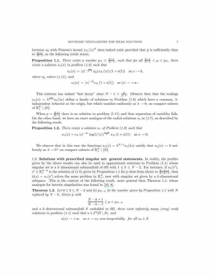
between u0 with Poisson’s kernel xN/|x|N does indeed exist provided that p is sufficiently close

to N+1N−1 , as the following result states.

Proposition 1.1. There exists a number pN > N+1N−1 , such that for all N+1

N−1 < p < pN , there

exists a solution u1(x) to problem (1.8) such that

u1(x) = |x|−2

p−1 φp(xN/|x|) (1 + o(1)) as x→ 0,

where φp solves (1.11), and

u1(x) = |x|−NxN (1 + o(1)) as |x| → +∞ .

This solution has indeed “fast decay” since N − 1 > 2p−1 . Observe then that the scalings

uλ(x) = λ2

p−1u1(λx) define a family of solutions to Problem (1.8) which have a common, λ-independent behavior at the origin, but which vanishes uniformly as λ→ 0, on compact subsetsof R

N+ \ 0.

When p = N+1N−1 there is no solution to problem (1.11) and thus separation of variables fails.

On the other hand, we have an exact analogue of the radial solutions u1 in (1.7), as described bythe following result.

Proposition 1.2. There exists a solution u1 of Problem (1.9) such that

u1(x) = cN |x|−N log(1/|x|)1−N

2 xN (1 + o(1)) as x→ 0.

We observe that in this case the functions uλ(x) = λN−1u1(λx) satisfy that uλ(x) → 0 uni-formly as λ→ 0+ on compact subsets of R

N+ \ 0.

1.3. Solutions with prescribed singular set: general statements. In reality, the profilesgiven by the above results can also be used to approximate solutions to Problem (1.1) whosesingular set is a k dimensional submanifold of ∂Ω with 1 ≤ k ≤ N − 2. For instance, if u1(x

′),

x′ ∈ RN−k+ is the solution of (1.8) given by Proposition 1.1 for p close from above to N−k+1

N−k−1 , then

u(x) = u1(x′) solves the same problem in R

N+ , now with singular set given by a k-dimensional

subspace. This is the content of the following result, more general than Theorem 1.1, whoseanalogue for interior singularities was found in [10, 8].

Theorem 1.2. Let 0 ≤ k ≤ N − 2 and let pN−k be the number given by Proposition 1.1 with Nreplaced by N − k. Given p with

N − k + 1

N − k − 1≤ p < pN−k

and a k-dimensional submanifold S embedded in ∂Ω, there exist infinitely many (very) weaksolutions to problem (1.1) such that u ∈ C2(Ω \ S), and

u(x) → +∞ as x→ x0 non-tangentially, for all x0 ∈ S.

6 MANUEL DEL PINO, MONICA MUSSO, FRANK PACARD

When k = 0, we agree that S is a finite set of isolated points, so that Theorem 1.1 is recovered.In reality, the solutions found arise as continua, depending on as many real parameters as numberof points lie in S. When k ≥ 1, the solutions we construct are infinite dimensional families. Theconstruction actually allows much more: For instance, when p = N+1

N−1 , the number of points ofthe singular set can be taken to infinity, to total a dense subset of any given closed set A of ∂Ω,which can be properly called its singular set. In fact, since the solutions we are interested inare smooth in Ω, it is natural to define the singular set of a very weak solution u of (1.1) as thecomplement in ∂Ω of the set of points x ∈ ∂Ω in a neighborhood of which u is smooth. Observethat, by definition, the singular set of u is a closed subset of ∂Ω. We have the validity of thefollowing general result.

Theorem 1.3. Let 0 ≤ k ≤ N − 2, and N−k+1N−k−1 ≤ p < pN−k. Let us consider a nonempty closed

subset A of ∂Ω, which contains a sequence of k-dimensional embedded submanifolds Si, i ∈ N,which are also disjoint and satisfy that S := ∪iSi is dense in A. Then, there exists a positivevery weak solution of Problem (1.1) whose singular set is exactly A, and such that

u(x) → +∞ as x→ x0 non-tangentially, for all x0 ∈ S,

and

u(x) → 0 as x→ x0 non-tangentially, for all x0 ∈ ∂Ω \ S.

This last result and the underlying construction have interesting consequences: for instance,for p larger than but close enough to N+1

N−1 , there are infinitely many very weak solutions of (1.1)

whose singular set is any prescribed closed subset of ∂Ω, but such that u ∈ W 1,q0 (Ω) for any

1 < q < N p−1

p+1 . Therefore, even though u is not identically equal to 0 at each point of ∂Ω, we cansay that u = 0 on ∂Ω in appropriate sense of traces.

The proof of these results relies on two basic ingredients: one is the construction of the basiccells of Propositions 1.1 and 1.2, which we carry our in §2. The other ingredient is the analysisof invertibility of Laplace’s operator for right hand sides that involve singular behavior near apoint or an embedded manifold of the boundary. After this analysis, which is carried out in §3,the proof of Theorem 1.2 then follows from a fixed point argument. The result of Theorem 1.3 isa consequence of an inductive construction taken to the limit under suitable control.

2. The half-space case: proofs of Propositions 1.1 and 1.2

It is natural and convenient to look for solutions of (1.8) or (1.9) of the form

u(x) = |x|−2

p−1 φ(− log |x|, x/|x|),

so that the equation ∆u+ up = 0 reads in terms of φ(t, θ), t ∈ R, θ ∈ SN−1+ , as

∂2t φ−

(

N − 2p+1

p−1

)

∂tφ−p+1

p−1

(

N −p+1

p−1

)

φ+ (∆SN−1 +N − 1) φ+ φp = 0. (2.1)

BOUNDARY SINGULARITIES FOR WEAK SOLUTIONS 7

2.1. Proof of Proposition 1.2. When p = N+1N−1 , in the language of equation (2.1), problem

(1.9) becomes

∂2t φ+N ∂tφ+ (∆SN−1 +N − 1) φ+ φ

N+1

N−1 = 0 in (t∗,∞) × SN−1+

φ > 0 in (t∗,∞) × SN−1+

φ = 0 on (t∗,∞) × ∂SN−1+ .

(2.2)

We allow here t∗ > 0 to be a parameter, which we will choose later to be large. To get a solutionof problem (1.9) we actually need t∗ = 0, but this is simply achieved by a translation of φ in thet-variable.

The idea is now to look for a solution of this equation of the form

φ(t, θ) = aN t−bN ϕ1(θ) + ψ(t, θ), (2.3)

where aN , bN are positive constants to be fixed below, and ϕ1 denotes the eigenfunction of−∆SN−1

+

associated to the eigenvalue N − 1 and normalized so that its L2-norm is equal to

1. Explicitly,

ϕ1(θ) =θN

(

∫

SN−1

+

θ2N dσ)1/2

.

When substituting the function φ = aN t−bN ϕ1(θ) as an approximation for a solution of equation

(2.2), we see that for large t, the main order term in the error created is the function

E(t, θ) := NaNbN t−b−1 ϕ1(θ) − |aN t−bN ϕ1(θ)|N+1

N−1 .

We make the following choice for the numbers aN and bN :

bN =N−1

2, aN =

[

2

N(N − 1)

∫

SN−1

+

ϕ2N

N−1

1 dσ

]−N−1

2

.

This election achieves the L2-orthogonality of E to ϕ1 for all t, namely∫

SN−1

+

E(t, ·)ϕ1 dσ = 0 for all t > t∗.

We fix these values in what follows. In terms of ψ in (2.3), equation (2.2) now reads

∂2t ψ +N ∂tψ + (∆SN−1 +N − 1) ψ + bN (bN + 1) aN t−bN−2 ϕ1−

NbNaN t−bN−1 ϕ1 + |aN t−bN ϕ1 + ψ|N+1

N−1 = 0,

ψ = 0 on (t∗,∞) × ∂SN−1+ .

We further decompose

ψ(t, θ) = f2(t)ϕ1(θ) + ψ1(t, θ) (2.4)

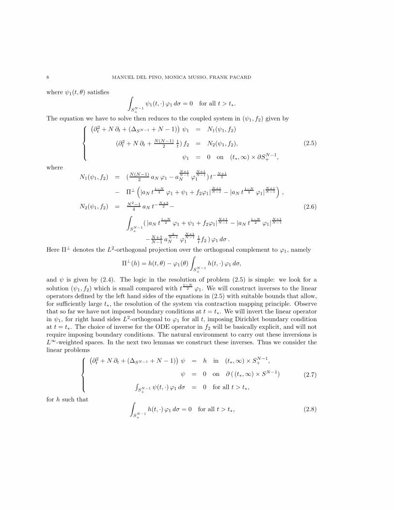
8 MANUEL DEL PINO, MONICA MUSSO, FRANK PACARD

where ψ1(t, θ) satisfies∫

SN−1

+

ψ1(t, ·)ϕ1 dσ = 0 for all t > t∗.

The equation we have to solve then reduces to the coupled system in (ψ1, f2) given by

(

∂2t +N ∂t + (∆SN−1 +N − 1)

)

ψ1 = N1(ψ1, f2)

(∂2t +N ∂t + N(N−1)

21t ) f2 = N2(ψ1, f2),

ψ1 = 0 on (t∗,∞) × ∂SN−1+ ,

(2.5)

where

N1(ψ1, f2) = (N(N−1)2 aN ϕ1 − a

N+1

N−1

N ϕN+1

N−1

1 ) t−N+1

2

− Π⊥(

|aN t1−N

2 ϕ1 + ψ1 + f2ϕ1|N+1

N−1 − |aN t1−N

2 ϕ1|N+1

N−1

)

,

N2(ψ1, f2) = N2−14 aN t−

N+3

2 −∫

SN−1

+

( |aN t1−N

2 ϕ1 + ψ1 + f2ϕ1|N+1

N−1 − |aN t1−N

2 ϕ1|N+1

N−1

−N+1N−1 a

2N−1

N ϕN+1

N−1

11t f2 )ϕ1 dσ .

(2.6)

Here Π⊥ denotes the L2-orthogonal projection over the orthogonal complement to ϕ1, namely

Π⊥(h) = h(t, θ) − ϕ1(θ)

∫

SN−1

+

h(t, ·)ϕ1 dσ,

and ψ is given by (2.4). The logic in the resolution of problem (2.5) is simple: we look for a

solution (ψ1, f2) which is small compared with t1−N

2 ϕ1. We will construct inverses to the linearoperators defined by the left hand sides of the equations in (2.5) with suitable bounds that allow,for sufficiently large t∗, the resolution of the system via contraction mapping principle. Observethat so far we have not imposed boundary conditions at t = t∗. We will invert the linear operatorin ψ1, for right hand sides L2-orthogonal to ϕ1 for all t, imposing Dirichlet boundary conditionat t = t∗. The choice of inverse for the ODE operator in f2 will be basically explicit, and will notrequire imposing boundary conditions. The natural environment to carry out these inversions isL∞-weighted spaces. In the next two lemmas we construct these inverses. Thus we consider thelinear problems

(

∂2t +N ∂t + (∆SN−1 +N − 1)

)

ψ = h in (t∗,∞) × SN−1+ ,

ψ = 0 on ∂ ( (t∗,∞) × SN−1)∫

SN−1

+

ψ(t, ·)ϕ1 dσ = 0 for all t > t∗,

(2.7)

for h such that∫

SN−1

+

h(t, ·)ϕ1 dσ = 0 for all t > t∗, (2.8)

BOUNDARY SINGULARITIES FOR WEAK SOLUTIONS 9

and(

∂2t +N ∂t +

N(N−1)

2

1

t

)

f = g in (t∗,∞). (2.9)

We have the validity of the following results.

Lemma 2.1. There exists a constant c > 0 such that the following holds: Given σ ≥ 0, thereis a tσ > 0, with tσ > 0 if σ > 0 and tσ = 0 if σ = 0, such that, for all t∗ ≥ tσ, and allh ∈ C0((t∗,∞)×SN−1

+ ) that satisfies (2.8) and tσh ∈ L∞((t∗,∞)×SN−1+ ), there exists a solution

ψ = T1(h) of problem (2.7), which defines a linear operator of h and satisfies the estimate

‖tσ ψ‖L∞ + ‖tσ ∇θψ‖L∞ ≤ c ‖tσ h‖L∞ .

Lemma 2.2. Given σ > N−1

2 , there exist numbers tσ, cσ > 0 such that for all t∗ > tσ and all

g ∈ C0((t∗,∞)) satisfying tσg ∈ L∞((t∗,∞)), there exists a solution f = T2(g) of equation (2.9),which defines a linear operator of g and satisfies the estimate

‖tσ f‖L∞ ≤ cσ ‖t1+σ g‖L∞.

Before proceeding into the proofs of these lemmas, let us conclude the result.

Conclusion of the proof of Proposition 1.2. Let us fix in the above lemmas any number σsuch that

N−1

2< σ <

N+1

2

and t∗ > tσ. We obtain a solution of problem (2.5) if (ψ1, f2) solves the fixed point problem

(ψ1, f2) = M(ψ1, f2) := (T1(N1(ψ1, f2) ) , T2(N2(ψ1, f2) )), (2.10)

in the space of functions

(ψ, f) ∈ C0([t∗,∞) × SN−1+ ) × C0([t∗,∞))

for which the norm‖(ψ, f)‖µ = ‖tσ ψ‖∞ + µ‖tσf‖∞

is finite. Here µ < 1 is a positive number which we will fix later. T1, T2 are the operatorspredicted by Lemmas 2.1 and 2.2. It is directly checked that we have the pointwise estimates

|N1(ψ1, f2)| ≤ A[ t−N+1

2 + t−1|ψ1| + t−1|f2| ] ,

|N2(ψ1, f2)| ≤ A[ t−N+3

2 + t−1|ψ1| + tN−3

2 |f2|2 + |f2|

N+1

N−1 ] ,(2.11)

where A depends only on N , whenever ‖(ψ, f)‖µ ≤ µ. It follows that,

‖tσN1(ψ1, f2)‖∞ ≤ A [ tσ−N+1

2∗ + t−1

∗ ‖tσψ1‖∞ + t−1∗ ‖tσf2‖∞ ] ,

‖t1+σN2(ψ1, f2)‖∞ ≤ A [ tσ−N+1

2∗ + ‖tσψ1‖∞ + (t

N−1

2−σ

∗ + t1− 2σ

N−1

∗ )‖tσf2‖∞ ] .

(2.12)

These estimates, together with Lemmas 2.1 and 2.2, yield that if µ is chosen sufficiently small,depending only on σ and N , and t∗ is taken sufficiently large, then the operator M applies theball ‖(ψ, f)‖µ ≤ µ into itself. A similar estimates shows that, also, M is a contraction mapping

10 MANUEL DEL PINO, MONICA MUSSO, FRANK PACARD

with this norm inside this region. Hence there is a fixed point (ψ1, f2) in this ball. The solutionobtained this way renders the function

φ(t, θ) = aN t−N−1

2 ϕ1(θ) + f2(t)ϕ1(θ) + ψ1(t, θ)

positive in (t∗,+∞)×SN−1+ , and it is then a solution of problem (2.2). This completes the proof

of Proposition 1.2.

Next we carry out the proofs of the lemmas.

Proof of Lemma 2.1 . Let us consider first the case σ = 0, so that h is bounded. Withno loss of generality, we also assume t∗ = 0. We see then that problem (2.7) has at most onebounded solution. This can be shown for instance expanding a bounded solution of the equationwith h = 0 in eigenfunctions of the Laplace-Beltrami operator with zero boundary conditionson SN−1

+ . The coefficients in this expansion will be functions of t which correspond to boundedsolution of certain homogeneous ODE’s which only have the zero solution. Thus, we only haveto prove existence. To do so, let us consider, for any given number t2 > 0, the problem

(∂2t +N ∂t + (∆SN−1 +N − 1))ψ = h in (0, t2) × SN−1

+

ψ = 0 on ∂ ( (0, t2) × SN−1+ ).

(2.13)

This problem is uniquely solvable since it is just a rephrasing of a Dirichlet problem for theLaplacian in a half-annular region. Let us denote by ψ = ψt2 its unique solution. Since, byassumption, h(t, ·) is L2-orthogonal to ϕ1 for all t ∈ (0, t2), so is ψ.

It suffices to check that there exists a constant c > 0 independent of t2 ≥ 1 such that

‖ψ‖L∞([0,t2]×SN−1

+) ≤ c ‖h‖L∞([0,t2]×SN−1

+). (2.14)

Indeed, assuming this estimate is already proven, we use elliptic estimates together with Ascoli’stheorem to show that, as t2 tends to ∞, the sequence of functions ψt2 converges uniformly to afunction ψ solution of (2.7) which satisfies

‖ψ‖L∞([0,∞)×SN−1

+) ≤ c ‖h‖L∞([0,∞)×SN−1

+).

Elliptic estimates then imply that

‖∇ψ‖L∞([0,∞)×SN−1

+) + ‖ψ‖L∞([0,∞)×SN−1

+) ≤ c0 ‖h‖L∞([0,∞)×SN−1

+). (2.15)

The orthogonality conditions on ψ pass certainly to the limit, and existence of a solution withthe desired properties thus follows. It remains to prove the uniform estimate (2.14). We argueby contradiction. Since the result is certainly true when t2 remains bounded, we assume thatthere exists a sequence t2 = t2,i tending to ∞, functions h = hi and ψi corresponding solutionsto problem (2.13) for which

‖ψi‖L∞([0,t2,i]×SN−1

+) = 1 and lim

i→∞‖hi‖L∞([0,t2,i]×SN−1

+) = 0.

We choose ti ∈ (0, t2,i) where ‖ψi‖L∞([t1,i,t2,i]×SN−1

+) is achieved and define

ψi(t, θ) = ψi(t+ ti, θ)

BOUNDARY SINGULARITIES FOR WEAK SOLUTIONS 11

Using elliptic estimates together with Ascoli’s theorem, we can extract from (ψi)i some subse-

quence which converges uniformly on compact sets to ψ, a bounded solution of

(∂2t +N ∂t + (∆SN−1 +N − 1)) ψ = 0 (2.16)

which is either defined on [0,∞)×SN−1+ , on (−∞, 0]×SN−1

+ or on (−∞,∞)×SN−1+ . Furthermore,

‖ψ‖L∞ = 1 (2.17)

with ψ having 0 boundary data. Furthermore ψ(t, ·) is L2-orthogonal to ϕ1, for all t. Eigenfunc-

tion decomposition of ψ(t, ·) for the Laplace-Beltrami operator yields that there is non nontrivialbounded solution of (2.16) and this contradicts (2.17). This completes the proof of the uniformestimate, and thus existence of a unique bounded solution of (2.7) with the desired estimatefollows. This solution of course defines a linear operator on bounded h.

To establish the result for σ > 0 and t∗ > 0 sufficiently large, let us write

h = t−σ h and ψ = t−σ ψ

so that h is bounded. (2.7) reduces to

(∂2t +N ∂t + (∆SN−1 +N − 1)) ψ +

(

σ(σ+1)

t2−

Nσ

t

)

ψ −2σ

t∂tψ = h (2.18)

We can estimate

‖(

σ(σ+1)

t2−

Nσ

t

)

ψ −2σ

t∂tψ‖L∞([t∗,∞)×SN−1

+) ≤

µ(

‖∇ψ‖L∞([t∗,∞)×SN−1

+) + ‖ψ‖L∞([t∗,∞)×SN−1

+)

)

where µ can be taken as small as we wish, after choosing t∗ ≥ tσ with tσ large enough. Theresolution of (2.18) with the desired bound then follows from that of (2.7) with σ = 0 togetherwith a direct linear perturbation argument. This finishes the proof.

Proof of Lemma 2.2 . Observe that a right inverse for the operator ∂2t + N ∂t on [t∗,∞) is

given by

G(g)(t) = −

∫ ∞

t

e−Nζ

∫ ζ

t∗

eNs g(s) ds dt

One checks that

‖tσ G(g)‖L∞((t∗,+∞)) ≤1

N |σ|

(

1 −(σ+1)

Nt∗

)−1

‖t1+σg‖L∞((t∗,+∞))

provided Nt∗ − 1 − σ > 0. This follows at once from the computation∫ t

t∗

eNs s−σ−1 ds =[

1

NeNs s−σ−1

]t

t∗+

σ+1

N

∫ t

t∗

eNs s−σ−2 ds

≤1

NeNt t−σ−1 +

1+σ

N t∗

∫ t

t∗

eNs s−σ−1 ds

12 MANUEL DEL PINO, MONICA MUSSO, FRANK PACARD

and hence(

1 −σ+1

N t∗

)∫ t

t∗

eNs s−σ−1 ds ≤1

NeNt t−σ−1.

The result of the lemma then follows from a simple linear perturbation argument, provided t∗ > 0is chosen so that

N(N−1)

2‖tσ

1

tG(g)‖L∞((t∗,+∞)) ≤

1

2‖t1+σg‖L∞((t∗,+∞)),

and the result is concluded. 2

2.2. Proof of Proposition 1.1. Recall that, when p ∈ ( N+1

N−1 ,N+1

N−3 ) the Mountain Pass Lemmayields the existence of φp, a nontrivial positive solution of (1.11). This solution then induces asolution

up(x) := |x|−2

p−1 φp(x/|x|),

of Problem (1.8), for which this time we emphasize its dependence on p. We have to show thatthere exists a solution of (1.8) which is asymptotic to up near 0 and it is asymptotic to

u∞(x) := |x|−N xN

at infinity. Let us consider a smooth cut-off function χ which is equal to 0 in B1(0) and it isidentically equal to 1 in R

N\B2(0). We will consider the function up(1−χ) as a first approximation

for the solution we are looking for. Since, we recall, φp approaches zero uniformly as p ↓ N+1N−1 ,

then the same is true for u0,p away from the origin. The result of the proposition relies on aperturbation procedure, and this is the reason why we can only show the for exponents p closeto N

N−1 . To carry out this scheme, we shall build a right inverse for the Laplacian relative to thefollowing doubly weighted space:

Definition 2.1. Given δ, δ′ ∈ R, the space L∞δ,δ′(RN

+ ) is defined to be the space of functions

u ∈ L∞loc(R

N+ ) for which the following norm

‖u‖L∞

δ,δ′(RN

+) = ‖|x|−δ u‖L∞(B+(1)) + ‖|x|−δ′

u‖L∞(RN+−B+(1))

is finite.

Hence δ controls the behavior of the function near 0 and δ′ the behavior of the function nearinfinity. Let us consider the problem

∆u = |x|−2f in RN+

u = 0 on ∂RN+ \ 0.

(2.19)

We have the validity of the following result.

Lemma 2.3. Let δ ∈ (1 −N, 1) and δ′ ∈ (−N, 1 −N) be given. There is a constant c > 0 suchthat for each f ∈ L∞

δ,δ′(RN+ ), there exists a solution u = G(f) of problem (2.19), which defines a

linear operator in f and can be decomposed as

u = u+ aχu∞

BOUNDARY SINGULARITIES FOR WEAK SOLUTIONS 13

with|a| + ‖u‖L∞

δ,δ′≤ c‖f‖L∞

δ,δ′.

Proof. Let us observe that δ (N − 2 + δ) < N − 1 precisely when δ ∈ (1 −N, 1). Therefore, wecan define ϕ∗ = ϕN,δ to be the unique, positive solution of

− (∆SN−1 + δ (δ +N − 2)) ϕ∗ = 1 in SN−1+

ϕ∗ = 0 on ∂SN−1+ .

A direct computation shows that

− |x|2 ∆RN (|x|δ ϕ∗(θ)) = c|x|δ. (2.20)

Assume that f ∈ L∞δ,δ′(RN

+ ). Given r1 < 1 < r2, we can solve the equation |x|2 ∆u = f in

RN+ ∩ (Br2

−Br1), with 0 boundary conditions. We use the function x 7−→ ϕ∗(x) |x|

δ as a barrierto prove the pointwise estimate

|u| ≤ c ‖f‖L∞

δ,δ′(RN

+) |x|

δ

in RN+ ∩ (Br2

−Br1). Furthermore, given δ ∈ (1 −N, 1) we can use the function x 7−→ ϕ∗(x) |x|

δ

as a barrier to prove the estimate

|u| ≤ c ‖f‖L∞

δ,δ′(RN

+) |x|

δ

in RN+ ∩ (Br2

−Br1).

We use elliptic regularity theory as well as Ascoli’s theorem to pass to the limit as r1 tendsto 0 and r2 tends to ∞. We obtain a solution u of problem (2.19) which satisfies the pointwiseestimates

|u| ≤ c ‖f‖L∞

δ,δ′(RN

+) |x|

δ

in (RN+ ∩B1) − 0, and

|u| ≤ c ‖f‖L∞

δ,δ′(RN

+) |x|

δ

in RN+ ∩ (RN −B1). Finally, the decomposition of the solution u at infinity into

u = u+ a u∞

where the function u satisfies|u| ≤ c ‖f‖L∞

δ,δ′(RN

+) |x|

δ′

follows easily from Green’s representation formula. Moreover, we can directly compute the valueof a. Indeed, integration of the equation over B+

r := RN+ ∩Br yields, for r large enough,

∫

B+r

f |x|−2 dx =

∫

∂B+r

∂ru dσ =

∫

SN−1

+

(∂ru)(r θ) rN−1 dσ − a (N − 1)

∫

SN−1

+

θN dσ

Passing to the limit as r tends to ∞, we obtain the identity

a (N − 1)

∫

SN−1

+

θN dσ = −

∫

RN+

f |x|−2 dx, (2.21)

14 MANUEL DEL PINO, MONICA MUSSO, FRANK PACARD

and the proof is concluded.

Conclusion of the proof of Proposition 1.1. To find a solution of problem (1.8), we write

u = (1 − χ)up + v,

where χ is a smooth cut-off function which is equal to 0 in B1 and identically equal to 0 inR

N −B2. Let us fix numbers δ ∈ (1 −N, 1), δ′ ∈ (−N, 1−N) and let G be the operator definedin Lemma 2.3. Then, we obtain a solution with the required properties if v solves the fixed pointproblem

v = −G(

|x|2(∆(1 − χ) up + |(1 − χ) up + v|p))

(2.22)

in the space L∞δ,δ′((RN

+ − 0) ⊕ Span χu∞), and (1 − χ)up + v > 0.

Let us observe that there exists a constant c0 = c(N, δ, δ′) > 0 such that

‖|x|2 (∆((1 − χ) up) + ((1 − χ) up)p)‖L∞

δ,δ′(RN

+−0) ≤ c0 ‖φp‖C2(SN−1

+). (2.23)

Indeed, since ∆up + upp = 0 we have

∆((1 − χ) up) + ((1 − χ) up)p = −∆χ up − 2∇χ · ∇up + (1 − χ− (1 − χ)p)∆up

and the estimate follows at once.

On the other hand, if we assume that p is sufficiently close to N+1N−1 from above, we have that

‖φp‖C2(SN−1

+) ≤ 1,

and also

δ > −2

p−1and δ′ > p (1 −N) + 2.

Under these constraints, it is not hard to check the existence of a constant c = c(N, δ, δ′) > 0such that

‖|x|2(|(1 − χ) up + v2|p − |(1 − χ) up + v1|

p)‖L∞

δ,δ′(RN

+−0)

≤ c ‖φp‖C2(SN−1

+) ‖v2 − v1‖L∞

δ,δ′(RN

+−0)⊕Span χ u∞

(2.24)

for all v2, v1 ∈ L∞δ,δ′(RN

+ − 0)⊕ Spanχu∞ satisfying

‖vi‖L∞

δ,δ′((RN

+−0)⊕Span χ u∞) ≤ 2 c0 ‖φp‖C2(SN−1

+).

Using estimates (2.23), (2.24) and Lemma 2.3, the existence of a solution to the fixed pointproblem (2.22) can then be obtained by contraction mapping principle in the ball of radius2 c0 ‖φp‖C2(SN−1

+) in the space L∞

δ,δ′((RN+ − 0)⊕ Span χu∞), provided that p is chosen larger

than (but close enough to) N+1N−1 . Let us denote by vp this fixed point.

Since δ > 1 − N , we have |vp| << up near 0 and hence the solution u := (1 − χ) up + vp issingular and positive near 0. We now prove that u := (1 − χ) up + vp is also positive at infinity.Indeed, the function vp can be written as

vp = vp + ap χu∞

BOUNDARY SINGULARITIES FOR WEAK SOLUTIONS 15

where, according to formula (2.21), ap can be computed as

ap (N − 1)

∫

SN+

θN dσ =

∫

RN+

(∆(1−χ) up + |(1−χ) up + vp|p) dx =

∫

RN+

|(1−χ) up + vp|p dx. > 0

This implies that ap > 0, and by the maximum principle, it is now easy to check that u > 0 inR

N+ − 0. This completes the proof of Proposition 1.1.

2.3. Some open questions. The results of proof of Propositions 1.1 and 1.2 and their parallelwith the radial case and p close to N

N−2 , to which we recall ODE phase plane analysis applies,lead us naturally to several questions concerning existence of solutions of ∆u + up = 0 on thepunctured half space R

N+ − 0 with 0 boundary data. We list some of them next.

Question 1. We believe that the solution u1 which has been obtained in Proposition 1.1 for pclose to N+1

N−1 should actually exist for all p ∈ (N+1N−1 ,

N+2N−2 ).

Question 2. When p = N+2N−2 , we believe that there exists a one parameter family of solutions of

the formu(x) = |x|

2−N2 v(− log |x|, θ)

where t 7−→ v(t, ·) is periodic. This one-parameter family of solution corresponds to the wellknow periodic solutions for the singular Yamabe problem and also to Delaunay surfaces in thecontext of constant mean curvature surfaces.

Question 3. When p > N+2N−2 , N ≥ 3, we believe that there exists a solution of ∆u + up = 0

defined on RN+ which is identically equal to 0 on ∂R

N+ and which is asymptotic to u0 in (1.10)

at ∞. This solution should correspond to the smooth radially symmetric solution of the same

equation which is defined on the whole space and decays like |x|−2

p−1 at infinity, when p > N+2N−2 .

Question 4. Are there singular solutions when p ≥ N+1N−3 , N ≥ 4? In this regime separation of

variables in general fails.

Some partial answer to this question is given in [3].

3. The bounded domain case: proofs of Theorems 1.2 and 1.3

The proof of our main results relies on two basic ingredients: one is the, already established,existence of the “basic cells” given by Propositions 1.1 and 1.2 which we will use to constructapproximations to singular solutions. Another important ingredient, on which we elaborate inthe next two subsections, is the analysis of invertibility of Laplace’s operator, for right hand sidesexhibiting a controlled singular behavior on a given embedded submanifold of ∂Ω, in the samespirit to that of Lemma 2.3. Then we will use a fixed point scheme analogous to that in the proofof Proposition 1.1.

For notational convenience, we will assume in what follows that Ω is actually a subset of RN ,

and that S is a smooth embedded submanifold of ∂Ω ⊂ RN with dimension k. We define

N = n+ k.

16 MANUEL DEL PINO, MONICA MUSSO, FRANK PACARD

We start by setting up a suitable description of the space and Laplacian operator in naturalcoordinates associated to S. While the analysis below is done for k ≥ 1, it applies equally wellto the point-singularity case k = 0, being actually simpler.

3.1. Local coordinate system. In a neighborhood of a point p of S let us choose coordinatesy1, . . . , yk on S. Next we choose sections E1, . . . , En−1 of the normal bundle of S in ∂Ω. We candefine Fermi coordinates in some tubular neighborhood of S in ∂Ω by using the exponential map,

F (p, (x1, . . . , xn−1)) = Exp∂Ωp (

∑

i

xi Ei(p))

for p in a neighborhood of p ∈ S and (x1, . . . , xn−1) in some neighborhood of 0 in Rn−1.

In these coordinates, it is well known that the induced metric gb on ∂Ω can be expanded as

gb = gRn−1 + gS + O(|x|)

where gS denotes the induced metric on S and x = (x1, . . . , xn−1).

Finally, to parameterize a neighborhood of a point of ∂Ω in Ω, we denote by En the normal(inward pointing) vector field about ∂Ω and again use the exponential map to define

G(q, xn) = q + xn En(q)

for q in a neighborhood of p in ∂Ω and xn ≥ 0 in some neighborhood of 0.

In these coordinates, it is well known that the Euclidan metric in Ω can be expanded as

gRn+k = dx2n + gb + O(xn).

Collecting these two expansions, we conclude that in these coordinates the (Euclidean) Lapla-cian can be expanded as

∆ = ∆NS + O(|x|)∇2 + O(1)∇ (3.1)

where x = (x1, . . . , xn) and ∆NS = ∆Rn +∆S is the Laplace Betrami operator on NS, the normalbundle of S in R

n.

3.2. Analysis of the Laplacian in weighted spaces. We want to prove a result in the samespirit as that of Lemma 2.3 in the current setting. To do this, we need to define weighted spaceson Ω\S, which have a controlled blow up rate as S is approached. Unlike those in Lemma 2.3, wechoose Holder spaces, which are more suitable to deal with linear perturbations which are secondorder operators. Let us define, for sufficiently small R > 0, half “balls” and “annuli”

B+(R) := (p, x) ∈ NS+ / |x| ∈ (0, R]

and

A+(R1, R2) := (p, x) ∈ NS+ / |x| ∈ [R1, R2]

B+(R) is roughly “half” of a tubular neighborhood of radius R of the manifold S, or just a ballin case that S reduces to a single points. We consider the following weighted space of functionsdefined on B+(R) \ S.

BOUNDARY SINGULARITIES FOR WEAK SOLUTIONS 17

Definition 3.1. The space Cℓ,αδ (B+(R) \ S) is the space of functions u ∈ Cℓ,α

loc (B+(R) \ S)) forwhich the norm

‖u‖Cℓ,α

δ(B+(R)\S) = sup

r∈(0,R)

r−δ ‖u(·, r ·)‖Cℓ,α(A+(r/2,r))

is finite.

We consider now the problem

∆NSu = |x|−2f in B+(R) \ S

u = 0 on ∂B+(R) \ S.(3.2)

We have the validity of the following result.

Lemma 3.1. Assume that δ ∈ (1 − n, 1). There exists a constant c > 0, independent of R > 0,

such that, for each f ∈ C0,αδ (B+(R) \ S), there is a solution u = Gδ,R (f) of problem (3.2) which

defines a linear operator of f and satisfies the estimate

‖u‖C2,α

δ(B+(R)\S) ≤ c‖f‖C0,α

δ(B+(R)\S) .

Proof. We only carry out the proof for R = 1 since the general case follows by scaling. First wesolve for each r ∈ (0, 1/2) the problem

∆NSu = |x|−2f in A+(r, 1)

u = 0 on ∂A+(r, 1)(3.3)

and call ur its unique solution. Maximum principle employed in a similar way as in Lemma 2.3,taking into account expansion (3.1), yield the a priori bound

|ur| ≤ c ‖f‖C0,α

δ(B+(1)\S) |x|

δ

where c = c(n, δ) > 0. Then, elliptic estimates applied on geodesic balls of radius r centered atdistance 2r from S give the following bound on the gradient of u

|∇ur| ≤ c ‖f‖C0,α

δ(B+(1)\S) |x|

δ−1

for some c = c(n, δ) > 0. Using Arzela’s theorem, we conclude that, for a sequence of radiitending to 0, the sequence ur converges to a function u which satisfies

|u| ≤ c ‖f‖C0,α

δ(B+(1)\S) |x|

δ

and solves (3.2) for R = 1. Again, elliptic estimates applied on geodesic balls of radius r centeredat distance 2r from S yield the bound

‖u‖C2,α

δ(B+(1)\S) ≤ c ‖f‖C2,α

δ(B+(1)\S)

for some constant c = c(n, δ) > 0. Uniqueness of the limit u is easy to get and we leave it to thereader. The proof is concluded. 2

18 MANUEL DEL PINO, MONICA MUSSO, FRANK PACARD

Next we will extend the previous result to the entire domain Ω \ S. To do so, we consider afunction

γ : Ω \ S −→ (0,∞)

smooth, positive, which in the above defined local coordinates coincides with |x| in a neighborhoodof S in Ω. This function will play the role of the function |x| defined in B+(R) \ S. We defineaccordingly weighted Holder spaces as follows.

Definition 3.2. We let the space Cℓ,αδ (Ω \ S) be that of functions u ∈ Cℓ,α

loc (Ω \ S) for which thenorm

‖u‖Cℓ,α

δ(Ω\S) = ‖u‖Cℓ,α

δ(B+(R)\S) + ‖u‖Cℓ,α(Ω\B+(R/2))

is finite.

We consider now the problem

∆u = γ−2f in Ω \ S

u = 0 on ∂Ω \ S.(3.4)

We have the following result, extension of Lemma 3.1.

Lemma 3.2. Assume that δ ∈ (1 − n, 1). There exists a constant c > 0 such that, for each

f ∈ C0,αδ (Ω \ S), there is a solution u = Gδ (f) of problem (3.4) which defines a linear operator

of f and satisfies the estimate

‖u‖C2,α

δ(Ω\S) ≤ c‖f‖C0,α

δ(Ω\S) .

Proof. The proof follows from Lemma 3.1, expansion (3.1) and a linear perturbation argument.First, we claim that the result of Lemma 3.1 remains true in B+(R) \ S if the operator ∆NS isreplaced by ∆ and if R is chosen small enough. Indeed, we have from (3.1) and Proposition 3.1

‖f − γ2 (∆ − ∆NS) Gδ,R(f)‖C0,α

δ(B+(R)\S) ≤ cR ‖f‖C0,α

δ(B+(R)\S).

The claim follows at once from a perturbation argument, provided that R is fixed small enough.We denote by Gδ,R the right inverse for ∆ in B+(R) \ S.

We consider a cut-off function χR which is equal to 1 in B+(R/2) \ S and equal to 0 inΩ \B+(R). We define

f := f − γ2 ∆(χRu1),

where u1 = Gδ,R(f). Observe that this function is supported in Ω \ B+(R/2). We have that

f ∈ C0,α(Ω) and

‖f‖C0,α(Ω) ≤ c‖f‖C0,α

δ(Ω\Γ)

for some constant c = c(n, δ, R) > 0.

Finally, we can solve∆u2 = γ−2f in Ω

u2 = 0 on ∂Ω.

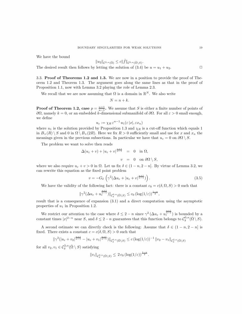
BOUNDARY SINGULARITIES FOR WEAK SOLUTIONS 19

We have the bound‖u2‖C2,α(Ω) ≤ c‖f‖C0,α(Ω\S).

The desired result then follows by letting the solution of (3.4) be u = u1 + u2. 2

3.3. Proof of Theorems 1.2 and 1.3. We are now in a position to provide the proof of The-orem 1.2 and Theorem 1.3. The argument goes along the same lines as that in the proof ofProposition 1.1, now with Lemma 3.2 playing the role of Lemma 2.3.

We recall that we are now assuming that Ω is a domain in RN . We also write

N = n+ k.

Proof of Theorem 1.2, case p = n+1n−1 . We assume that S is either a finite number of points of

∂Ω, namely k = 0, or an embedded k-dimensional submanifold of ∂Ω. For all ε > 0 small enough,we define

uε := χR εn−1 u1(ε |x|, εxn)

where u1 is the solution provided by Proposition 1.3 and χR is a cut-off function which equals 1in B+(R) \ S and 0 in Ω \B+(2R). Here we fix R > 0 sufficiently small and use for x and xn themeanings given in the previous subsections. In particular we have that uε = 0 on ∂Ω \ S.

The problem we want to solve then reads

∆(uε + v) + |uε + v|n+1

n−1 = 0 in Ω,

v = 0 on ∂Ω \ S,

where we also require uε + v > 0 in Ω. Let us fix δ ∈ (1 − n, 2 − n]. By virtue of Lemma 3.2, wecan rewrite this equation as the fixed point problem

v = −Gδ

(

γ2(∆uε + |uε + v|n+1

n−1 ))

. (3.5)

We have the validity of the following fact: there is a constant c0 = c(δ,Ω, S) > 0 such that

‖γ2(∆uε + un+1

n−1

ε )‖C0,α

δ(Ω\S) ≤ c0 (log(1/ε))

1−n2 ,

result that is a consequence of expansion (3.1) and a direct computation using the asymptoticproperties of u1 in Proposition 1.2.

We restrict our attention to the case where δ ≤ 2 − n since γ2 (∆uε + un+1

n−1

ε ) is bounded by a

constant times |x|2−n near S, and δ ≤ 2−n guarantees that this function belongs to C0,αδ (Ω \S).

A second estimate we can directly check is the following: Assume that δ ∈ (1 − n, 2 − n] isfixed. There exists a constant c = c(δ,Ω, S) > 0 such that

‖γ2(|uε + v2|n+1

n−1 − |uε + v1|n+1

n−1 )‖C0,α

δ(Ω\S) ≤ c (log(1/ε))−1 ‖v2 − v1‖C2,α

δ(Ω\S)

for all v2, v1 ∈ C2,αδ (Ω \ S) satisfying

‖vi‖C2,α

δ(Ω\S) ≤ 2 c0 (log(1/ε))

1−n2 .

20 MANUEL DEL PINO, MONICA MUSSO, FRANK PACARD

The above estimates allow an application of contraction mapping principle in the ball of radius

2 c0 (log(1/ε))1−n

2 in C2,αδ (Ω\S) to predict existence of a solution to problem (3.5), which we denote

by vε.

Since δ > 1−n, we have |vε| << uε near S and hence the solution u := uε+vε is singular alongS and is positive near S. The maximum principle then implies that u > 0 in Ω. This completesthe proof of Theorem 1.2 in the case p = n+1

n−1 .

The proof of Theorem 1.3, case p = n+1n−1 . This proof uses similar arguments together

with an induction process. By assumption, A is closed and contains a sequence of k-dimensionalsubmanifolds Si, i ∈ N such that ∪iSi is dense in A. We define inductively the sequence offunctions ui which are solutions of

∆ui + un+1

n−1

i = 0 (3.6)

in Ω, satisfy ui = 0 on ∂Ω − ∪ij=0Sj and are singular along ∪i

j=0Sj. Assume for example thatui−1 has already been constructed, then, we define

ui = ui−1 + εn−1i χri+1

u1(εi dist(·, Si))

where u1 is the solution provided by Proposition 1.3, ri is fixed small enough less than half thedistance from Si to ∪i−1

j=0Sj and εi > 0 is small enough. Applying a perturbation argument as

above, we can perturb ui into a solution ui = ui + vi of (3.6) for some function vi ∈ C2,αδ (Ω \

∪ij=0Sj). Taking εi small enough, we can ensure that

‖ui − ui−1‖L1(Ω) ≤ 2−i (3.7)

‖dist(·, ∂Ω)2 |ui − ui−1|n+1

n−1 ‖n+1

n−1

L1(Ω) ≤ 2−i (3.8)

and

‖γδvi‖L∞(Ω) ≤ 2−i (3.9)

where γ = dist(·, S) and where δ ∈ (1− n, 2− n] is fixed. Clearly (3.7) ensures that the sequence(ui)i converges in L1(Ω) to a function u. Moreover (3.7) and (3.8) imply that u is a weak solutionof (1.1). Finally, (3.9) implies that the nontangential limit of u at any point of S is equal to+∞.

Finally, we observe that, using Proposition 1.1 instead of Proposition 1.2, the results of Theo-rems 1.2 and 1.3 hold when p > n+1

n−1 , is sufficiently close to n+1n−1 . The only difference being that,

in the proof of the result corresponding to the one of Theorem 1.3, in addition to the properties(3.7) to (3.9) which ensure the convergence of the sequence of solutions in the appropriate space,we may also ask that the sequence converges in W 1,q(Ω), for some q close enough to 1. The proofsare concluded.

Acknowledgement

This work has been supported by grants Ecos/Conicyt C05E05, Fondecyt 1030840, 104936,and FONDAP.

BOUNDARY SINGULARITIES FOR WEAK SOLUTIONS 21

References

[1] H. Brezis and R. Turner, On a class of superlinear elliptic problems Commun. Partial Differ. Equations, 2(1977), 601-614.

[2] H. Beresticky, I. Capuzzo-Dolcetta, L. Nirenberg, Superlinear indefinite elliptic problems and nonlinear Li-

ouville theorems, Topol. Methods Nonlinear Anal., 4 (1994), 59-78.[3] M.F. Bidaut-Veron, A. Ponce and L. Veron, Boundary singularities of positive solutions of some nonlinear

elliptic equations, C. R. Acad. Sci. Paris, Ser. I 344, 2, (2007) 83-88[4] C.C. Chen and C.S. Lin, Existence of positive weak solutions with a prescribed singular set of semilinear

elliptic equations. J. Geom. Anal. 9 (1999), no. 2, 221–246.[5] S. Fakhi, New existence results for singular solutions of some semilinear elliptic equations. Comm. Partial

Differential Equations 25 (2000), no. 9-10, 1649–1668.[6] S. Fakhi, Positive solutions of ∆u + up = 0 whose singular set is a manifold with boundary. Calc. Var.

Partial Differential Equations 17 (2003), no. 2, 179–197.[7] B. Gidas and J. Spruck, Global and local behavior of positive solutions of nonlinear elliptic equations. Comm.

Pure Appl. Math. 34 (1981), no. 4, 525–598.[8] R. Mazzeo and F. Pacard, A construction of singular solutions for a semilinear elliptic equation using as-

ymptotic analysis. J. Differential Geom. 44 (1996), no. 2, 331–370.[9] F. Pacard, Existence and convergence of weak positive solutions of −∆u = uα in bounded domains of R

n,

n ≥ 3 C. R. Acad. Sci. Paris Sr. I Math. 315 (1992), no. 7, 793–798.

[10] F. Pacard, Existence and convergence of positive weak solutions of −∆u = un

n−2 in bounded domains of Rn,

n ≥ 3. Calc. Var. Partial Differential Equations 1, (1993), 243-265.[11] P. Quittner, and P. Souplet, A priori estimates and existence for elliptic systems via bootstrap in weighted

Lebesgue spaces. Arch. Ration. Mech. Anal. 174 (2004), no. 1, 49–81[12] P. Souplet, Optimal regularity conditions for elliptic problems via L

pδ-spaces, Duke Math. J. 127, (2005), no

1, 175-192.

M. del Pino

Departamento de Ingenierıa Matematica and CMM, Universidad de Chile, Casilla 170 Correo 3,Santiago, Chile.email : delpino@dim.uchile.cl,

M. Musso

Departamento de Matematica, Pontificia Universidad Catolica de Chile, Avda. Vicuna Mackenna4860, Macul, Chile and Dipartimento di Matematica, Politecnico di Torino, Corso Duca degliAbruzzi 24, 10129 Torino, Italy.email : mmusso@mat.puc.cl,

F. Pacard

Universite Paris 12 and Institut Universitaire de Franceemail : pacard@univ-paris12.fr