Semilinear Evolution Equations of Second Order via Maximal Regularity
20
Hindawi Publishing Corporation Advances in Difference Equations Volume 2008, Article ID 316207, 20 pages doi:10.1155/2008/316207 Research Article Semilinear Evolution Equations of Second Order via Maximal Regularity Claudio Cuevas 1 and Carlos Lizama 2 1 Departamento de Matem´ atica, Universidade Federal de Pernambuco, Avenue Prof. Luiz Freire, S/N, Recife, 50540-740 PE, Brazil 2 Departamento de Matem´ atica, Facultad de Ciencias, Universidad de Santiago de Chile, Casilla 307-Correo 2, Santiago, Chile Correspondence should be addressed to Carlos Lizama, [email protected] Received 26 October 2007; Revised 23 January 2008; Accepted 4 February 2008 Recommended by Alberto Cabada This paper deals with the existence and stability of solutions for semilinear second-order evolution equations on Banach spaces by using recent characterizations of discrete maximal regularity. Copyright q 2008 C. Cuevas and C. Lizama. This is an open access article distributed under the Creative Commons Attribution License, which permits unrestricted use, distribution, and reproduction in any medium, provided the original work is properly cited. 1. Introduction Let A be a bounded linear operator defined on a complex Banach space X. In this article, we are concerned with the study of existence of bounded solutions and stability for the semilinear problem Δ 2 x n − Ax n f n, x n , Δx n , n ∈ Z , 1.1 by means of the knowledge of maximal regularity properties for the vector-valued discrete time evolution equation Δ 2 x n − Ax n f n , n ∈ Z , 1.2 with initial conditions x 0 0 and x 1 0. The theory of dynamical systems described by the difference equations has attracted a good deal of interest in the last decade due to the various applications of their qualitative properties; see 1–5. In this paper, we prove a very general theorem on the existence of bounded solutions for the semilinear problem 1.1 on l p Z ; X spaces. The general framework for the proof of this statement uses a new approach based on discrete maximal regularity.
Transcript of Semilinear Evolution Equations of Second Order via Maximal Regularity

Hindawi Publishing CorporationAdvances in Difference EquationsVolume 2008, Article ID 316207, 20 pagesdoi:10.1155/2008/316207
Research ArticleSemilinear Evolution Equations of Second Ordervia Maximal Regularity
Claudio Cuevas1 and Carlos Lizama2
1Departamento de Matematica, Universidade Federal de Pernambuco, Avenue Prof. Luiz Freire, S/N,Recife, 50540-740 PE, Brazil
2Departamento de Matematica, Facultad de Ciencias, Universidad de Santiago de Chile,Casilla 307-Correo 2, Santiago, Chile
Correspondence should be addressed to Carlos Lizama, [email protected]
Received 26 October 2007; Revised 23 January 2008; Accepted 4 February 2008
Recommended by Alberto Cabada
This paper deals with the existence and stability of solutions for semilinear second-order evolutionequations on Banach spaces by using recent characterizations of discrete maximal regularity.
Copyright q 2008 C. Cuevas and C. Lizama. This is an open access article distributed underthe Creative Commons Attribution License, which permits unrestricted use, distribution, andreproduction in any medium, provided the original work is properly cited.
1. Introduction
Let A be a bounded linear operator defined on a complex Banach space X. In this article, weare concerned with the study of existence of bounded solutions and stability for the semilinearproblem
Δ2xn −Axn = f(n, xn,Δxn), n ∈ Z+, (1.1)
by means of the knowledge of maximal regularity properties for the vector-valued discretetime evolution equation
Δ2xn −Axn = fn, n ∈ Z+, (1.2)
with initial conditions x0 = 0 and x1 = 0.The theory of dynamical systems described by the difference equations has attracted
a good deal of interest in the last decade due to the various applications of their qualitativeproperties; see [1–5].
In this paper, we prove a very general theorem on the existence of bounded solutions forthe semilinear problem (1.1) on lp(Z+;X) spaces. The general framework for the proof of thisstatement uses a new approach based on discrete maximal regularity.

2 Advances in Difference Equations
In the continuous case, it is well known that the study of maximal regularity is veryuseful for treating semilinear and quasilinear problems (see, e.g., Amann [6], Denk et al. [7],Clement et al. [8], the survey by Arendt [9], and the bibliography therein). Maximal regularityhas also been studied in the finite difference setting. Blunck considered in [10, 11] maximalregularity for linear difference equations of first order; see also Portal [12, 13]. In [14], max-imal regularity on discrete Holder spaces for finite difference operators subject to Dirichletboundary conditions in one and two dimensions is proved. Furthermore, the authors inves-tigated maximal regularity in discrete Holder spaces for the Crank-Nicolson scheme. In [15],maximal regularity for linear parabolic difference equations is treated, whereas in [16] a char-acterization in terms of R-boundedness properties of the resolvent operator for linear second-order difference equations was given; see also the recent paper by Kalton and Portal [17],where they discussed maximal regularity of power-bounded operators and relate the discreteto the continuous time problem for analytic semigroups. However, for nonlinear discrete timeevolution equations like (1.1), this new approach appears not to be considered in the litera-ture.
The paper is organized as follows. Section 2 provides an explanation for the basic nota-tions and definitions to be used in the article. In Section 3, we prove the existence of boundedsolutions whose second discrete derivative is in lp (1 < p < +∞) for the semilinear problem(1.1) by using maximal regularity and a contraction principle. We also get some a priori es-timates for the solutions xn and their discrete derivatives Δxn and Δ2xn. Such estimates willfollow from the discrete Gronwall inequality [1] (see also [18, 19]). In Section 4, we give a cri-terion for stability of (1.1). Finally, in Section 5 we deal with local perturbations of the system(1.2).
2. Discrete maximal regularity
LetX be a Banach space. Let Z+ denote the set of nonnegative integer numbers and letΔ be theforward difference operator of the first order, that is, for each x : Z+ → X and n ∈ Z+, Δxn =xn+1 − xn. We consider the second-order difference equation
Δ2xn − (I − T)xn = fn, ∀n ∈ Z+,
x0 = x, Δx0 = x1 − x0 = y,(2.1)
where T ∈ B(X), Δ2xn = Δ(Δxn), and f : Z+ → X.Denote C(0) = I, the identity operator on X, and define
C(n) =[n/2]∑
k=0
(n
2k
)(I − T)k, for n = 1, 2, . . . , (2.2)
and C(n) = C(−n), for n = −1,−2, . . . . We define also S(0) = 0,
S(n) =[(n−1)/2]∑
k=0
(n
2k + 1
)(I − T)k, (2.3)
for n = 1, 2, . . . , and S(n) = −S(−n), for n = −1,−2, . . . .

C. Cuevas and C. Lizama 3
Considering the above notations, it was proved in [16] that the (unique) solution of (2.1)is given by
xm+1 = C(m)x + S(m)y + (S∗f)m. (2.4)
Moreover,
Δxm+1 = (I − T)S(m)x + C(m)y + (C∗f)m. (2.5)
The following definition is the natural extension of the concept of maximal regularityfrom the continuous case (cf., [16]).
Definition 2.1. Let 1 < p < +∞. One says that an operator T ∈ B(X) has discrete maximalregularity if KTf :=
∑nk=1(I − T)S(k)fn−k defines a bounded operatorKT ∈ B(lp(Z+, X)).
As a consequence of the definition, if T ∈ B(X) has discrete maximal regularity, then Thas discrete lp-maximal regularity, that is, for each (fn) ∈ lp(Z+;X)we have (Δ2xn) ∈ lp(Z+;X),where (xn) is the solution of the equation
Δ2xn − (I − T)xn = fn, ∀n ∈ Z+, x0 = 0, x1 = 0. (2.6)
Moreover,
Δ2xn =n−1∑
k=1
(I − T)S(k)fn−1−k + fn. (2.7)
We introduce the means
∥∥(x1, . . . , xn)∥∥R :=
12n
∑
εj∈{−1,1}n
∥∥∥∥∥
n∑
j=1
εjxj
∥∥∥∥∥ (2.8)
for x1, . . . , xn ∈ X.
Definition 2.2. LetX and Y be Banach spaces. A subsetT of B(X,Y ) is calledR-bounded if thereexists a constant c ≥ 0 such that
∥∥(T1x1, . . . , Tnxn)∥∥R ≤ c
∥∥(x1, . . . , xn)∥∥R (2.9)
for all T1, . . . , Tn ∈ T, x1, . . . , xn ∈ X, n ∈ N. The least c such that (2.9) is satisfied is called theR-bound of T and is denoted by R(T).
An equivalent definition using the Rademacher functions can be found in [7]. We notethat R-boundedness clearly implies boundedness. If X = Y , the notion of R-boundedness isstrictly stronger than boundedness unless the underlying space is isomorphic to aHilbert space[20, Proposition 1.17]. Some useful criteria for R-boundedness are provided in [7, 20, 21].

4 Advances in Difference Equations
Remark 2.3. (a) Let S,T ⊂ B(X,Y ) be R-bounded sets, then S + T := {S + T : S ∈ S, T ∈ T} isR-bounded.
(b) Let T ⊂ B(X,Y ) and S ⊂ B(Y,Z) be R-bounded sets, then S · T := {S ·T : S ∈ S,T ∈ T} ⊂ B(X,Z) is R-bounded and
R(S · T) ≤ R(S) · R(T). (2.10)
(c) Also, each subset M ⊂ B(X) of the form M = {λI : λ ∈ Ω} is R-bounded wheneverΩ ⊂ C is bounded. This follows from Kahane’s contraction principle (see [20, 22] or [7]).
A Banach space X is said to be UMD if the Hilbert transform is bounded on Lp(R, X) forsome (and then all) p ∈ (1,∞). Here, the Hilbert transform H of a function f ∈ S(R, X), theSchwartz space of rapidly decreasing X-valued functions, is defined by
Hf :=1πPV
(1t
)∗f. (2.11)
These spaces are also called HT spaces. It is a well-known theorem that the set of Banachspaces of class HT coincides with the class of UMD spaces. This has been shown by Bourgain[23] and Burkholder [24].
Recall that T ∈ B(X) is called analytic if the set{n(T − I)Tn : n ∈ N
}(2.12)
is bounded. For recent and related results on analytic operators we refer the reader to [25].The characterization of discrete maximal regularity for second-order difference equations byR-boundedness properties of the resolvent operator T reads as follows (see [16]).
Theorem 2.4. Let X be a UMD space and let T ∈ B(X) be analytic. Then, the following assertions areequivalent.
(i) T has discrete maximal regularity of order 2.
(ii){(λ − 1)2R((λ − 1)2, I − T) : |λ| = 1, λ /= 1
}is R-bounded.
Observe that from the point of view of applications, the above-given characteriza-tion provides a workable criterion; see Section 4 below. We remark that the concept of R-boundedness plays a fundamental role in recent works by Clement-Da Prato [26], Clementet al. [22], Weis [27, 28], Arendt-Bu [20, 29], and Keyantuo-Lizama [30–32].
3. Semilinear second-order evolution equations
In this section, our aim is to investigate the existence of bounded solutions, whose seconddiscrete derivative is in �p for semilinear evolution equations via discrete maximal regularity.
Next, we consider the following second-order evolution equation:
Δ2xn −Axn = f(n, xn,Δxn
), n ∈ Z+, x0 = 0, x1 = 0, (3.1)
which is equivalent to
xn+2 − 2xn+1 + Txn = f(n, xn,Δxn
), ∀n ∈ Z+, x0 = 0, x1 = 0, (3.2)
where T := I −A.

C. Cuevas and C. Lizama 5
To establish the next result, we need to introduce the following assumption.
Assumption 3.1. Suppose that the following conditions hold.
(i) The function f : Z+ × X × X → X satisfy the Lipschitz condition on X × X, that isfor all z,w ∈ X × X and n ∈ Z+, we get ‖f(n, z) − f(n,w)‖X ≤ αn‖z − w‖X×X, whereα := (αn) ∈ l1(Z+).
(ii) f(·, 0, 0) ∈ l1(Z+, X).
We remark that the condition α ∈ l1(Z) in (i) is satisfied quite often in applications. Forexample, it appears when we study asymptotic behavior of discrete Volterra systems whichdescribe processes whose current state is determined by their entire history. These processesare encountered in models of materials with memory, in various problems of heredity or epi-demics, in theory of viscoelasticity, and in solving optimal control problems (see, e.g., [33, 34]).
We began with the following property which will be useful in the proof of our mainresult.
Lemma 3.2. Let (αn) be a sequence of positive real numbers. For all n, l ∈ Z+, one has
n−1∑
m=0
αm
(m−1∑
j=0
αj
)l
≤ 1l + 1
(n−1∑
j=0
αj
)l+1
. (3.3)
Proof. Putting Am :=∑m−1
j=0 αj , we obtain
(l + 1)(Am+1 −Am
)Al
m =(Am+1 −Am
)(Al
m +Al−1m Am + · · · +AmA
l−1m +Al
m
)
≤(Am+1 −Am)
(Al
m+1 +Al−1m+1Am + · · · +Am+1A
l−1m +Al
m
)
= Al+1m+1 −Al+1
m .
(3.4)
Hence,
(l + 1)n−1∑
m=0
(Am+1 −Am
)Al
m ≤n−1∑
m=0
(Al+1
m+1 −Al+1m
)= Al+1
n . (3.5)
Denote by W2,p0 the Banach space of all sequences V = (Vn) belonging to l∞(Z+, X) such
that V0 = V1 = 0 and Δ2V ∈ lp(Z+, X) equipped with the norm |||V ||| = ‖V ‖∞ + ‖Δ2V ‖p. Wewill say that T ∈ B(X) is S-bounded if S ∈ l∞(Z+;X). With the above notations, we have thefollowing main result.
Theorem 3.3. Assume that Assumption 3.1 holds. In addition, suppose that T is S-bounded and thatit has discrete maximal regularity. Then, there is a unique bounded solution x = (xn) of (3.1) such that(Δ2xn) ∈ lp(Z+, X). Moreover, one has the following a priori estimates for the solution:
supn∈Z+
[∥∥xn
∥∥X +∥∥Δxn
∥∥X
]≤ 3M
∥∥f(·, 0, 0)∥∥1e
3M‖α‖1 ,
∥∥Δ2x∥∥p ≤ C
∥∥f(·, 0, 0)∥∥1e
6M‖α‖1 , 1 < p < +∞,
(3.6)
whereM := supn∈Z+‖S(n)‖ and C > 0.
6 Advances in Difference Equations
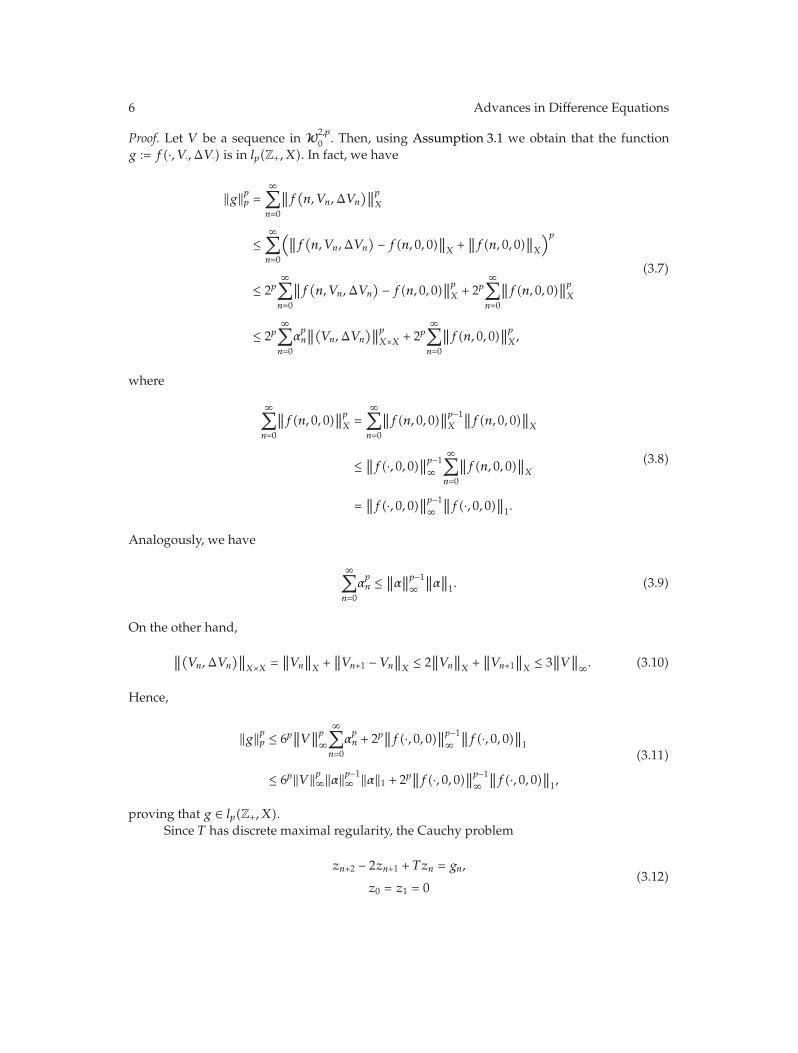
Proof. Let V be a sequence in W2,p0 . Then, using Assumption 3.1 we obtain that the function
g := f(·, V·,ΔV·) is in lp(Z+, X). In fact, we have
‖g‖pp =∞∑
n=0
∥∥f(n, Vn,ΔVn
)∥∥pX
≤∞∑
n=0
(∥∥f(n, Vn,ΔVn
)− f(n, 0, 0)
∥∥X +∥∥f(n, 0, 0)
∥∥X
)p
≤ 2p∞∑
n=0
∥∥f(n, Vn,ΔVn
)− f(n, 0, 0)
∥∥pX + 2p
∞∑
n=0
∥∥f(n, 0, 0)∥∥pX
≤ 2p∞∑
n=0
αpn
∥∥(Vn,ΔVn
)∥∥pX×X + 2p
∞∑
n=0
∥∥f(n, 0, 0)∥∥pX,
(3.7)
where
∞∑
n=0
∥∥f(n, 0, 0)∥∥pX =
∞∑
n=0
∥∥f(n, 0, 0)∥∥p−1X
∥∥f(n, 0, 0)∥∥X
≤∥∥f(·, 0, 0)
∥∥p−1∞
∞∑
n=0
∥∥f(n, 0, 0)∥∥X
=∥∥f(·, 0, 0)
∥∥p−1∞∥∥f(·, 0, 0)
∥∥1.
(3.8)
Analogously, we have
∞∑
n=0
αpn ≤∥∥α∥∥p−1∞∥∥α∥∥1. (3.9)
On the other hand,
∥∥(Vn,ΔVn
)∥∥X×X =
∥∥Vn
∥∥X +∥∥Vn+1 − Vn
∥∥X ≤ 2
∥∥Vn
∥∥X +∥∥Vn+1
∥∥X ≤ 3
∥∥V∥∥∞. (3.10)
Hence,
‖g‖pp ≤ 6p∥∥V∥∥p∞
∞∑
n=0
αpn + 2p
∥∥f(·, 0, 0)∥∥p−1∞∥∥f(·, 0, 0)
∥∥1
≤ 6p‖V ‖p∞‖α‖p−1∞ ‖α‖1 + 2p
∥∥f(·, 0, 0)∥∥p−1∞∥∥f(·, 0, 0)
∥∥1,
(3.11)
proving that g ∈ lp(Z+, X).Since T has discrete maximal regularity, the Cauchy problem
zn+2 − 2zn+1 + Tzn = gn,
z0 = z1 = 0(3.12)
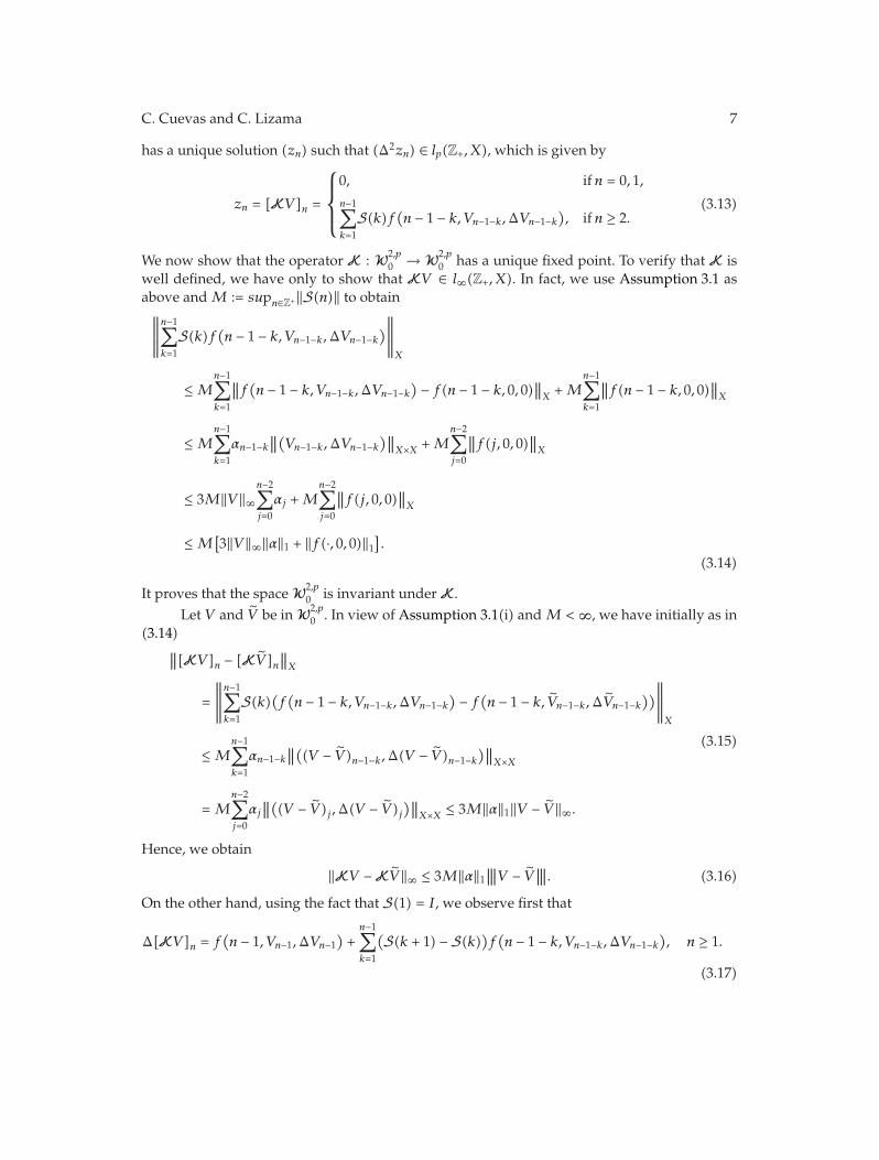
C. Cuevas and C. Lizama 7
has a unique solution (zn) such that (Δ2zn) ∈ lp(Z+, X), which is given by
zn = [KV ]n =
⎧⎪⎪⎨
⎪⎪⎩
0, ifn = 0, 1,n−1∑
k=1
S(k)f(n − 1 − k, Vn−1−k,ΔVn−1−k
), ifn ≥ 2.
(3.13)
We now show that the operator K : W2,p0 → W2,p
0 has a unique fixed point. To verify that K iswell defined, we have only to show that KV ∈ l∞(Z+, X). In fact, we use Assumption 3.1 asabove andM := supn∈Z+‖S(n)‖ to obtain∥∥∥∥∥
n−1∑
k=1
S(k)f(n − 1 − k, Vn−1−k,ΔVn−1−k
)∥∥∥∥∥X
≤ Mn−1∑
k=1
∥∥f(n − 1 − k, Vn−1−k,ΔVn−1−k
)− f(n − 1 − k, 0, 0)
∥∥X +M
n−1∑
k=1
∥∥f(n − 1 − k, 0, 0)∥∥X
≤ Mn−1∑
k=1
αn−1−k∥∥(Vn−1−k,ΔVn−1−k
)∥∥X×X +M
n−2∑
j=0
∥∥f(j, 0, 0)∥∥X
≤ 3M‖V ‖∞n−2∑
j=0
αj +Mn−2∑
j=0
∥∥f(j, 0, 0)∥∥X
≤ M[3‖V ‖∞‖α‖1 + ‖f(·, 0, 0)‖1
].
(3.14)
It proves that the space W2,p0 is invariant underK.
Let V and V be inW2,p0 . In view of Assumption 3.1(i) andM < ∞, we have initially as in
(3.14)∥∥[KV ]n − [KV ]n
∥∥X
=
∥∥∥∥∥
n−1∑
k=1
S(k)(f(n − 1 − k, Vn−1−k,ΔVn−1−k
)− f(n − 1 − k, Vn−1−k,ΔVn−1−k
))∥∥∥∥∥X
≤ Mn−1∑
k=1
αn−1−k∥∥((V − V )n−1−k,Δ(V − V )n−1−k
)∥∥X×X
= Mn−2∑
j=0
αj
∥∥((V − V )j ,Δ(V − V )j)∥∥
X×X ≤ 3M‖α‖1‖V − V ‖∞.
(3.15)
Hence, we obtain
‖KV −KV ‖∞ ≤ 3M‖α‖1∣∣∣∣∣∣V − V
∣∣∣∣∣∣. (3.16)
On the other hand, using the fact that S(1) = I, we observe first that
Δ[KV ]n = f(n − 1, Vn−1,ΔVn−1
)+
n−1∑
k=1
(S(k + 1) − S(k)
)f(n − 1 − k, Vn−1−k,ΔVn−1−k
), n ≥ 1.
(3.17)

8 Advances in Difference Equations
Since S(2) = 2I, we get
Δ2[KV ]n = f(n, Vn,ΔVn
)− f(n − 1, Vn−1,ΔVn−1
)+(S(2) − I
)f(n − 1, Vn−1,ΔVn−1
)
+n−1∑
k=1
(S(k + 2) − 2S(k + 1) + S(k))f
(n − 1 − k, Vn−1−k,ΔVn−1−k
)
= f(n, Vn,ΔVn) +
n−1∑
k=1
(S(k + 2) − 2S(k + 1) + TS(k)
)f(n − 1 − k, Vn−1−k,ΔVn−1−k
)
+n−1∑
k=1
(I − T)S(k)f(n − 1 − k, Vn−1−k,ΔVn−1−k
).
(3.18)
Taking into account that zn+1 = (S∗g)n is solution of (3.12), we get the following identity:
n−1∑
k=1
(S(k + 2) − 2S(k + 1) + TS(k)
)f(n − 1 − k, Vn−1−k,ΔVn−1−k
)= 0. (3.19)
Using (3.19), we obtain for n ≥ 1
Δ2[KV ]n = f(n, Vn,ΔVn
)+
n−1∑
k=1
(I − T)S(k)f(n − 1 − k, Vn−1−k,ΔVn−1−k
), (3.20)
whence, for n ≥ 1,
Δ2[KV ]n −Δ2[KV ]n
= f(n, Vn,ΔVn
)− f(n, Vn,ΔVn
)
+n−1∑
k=1
(I − T)S(k)(f(n − 1 − k, Vn−1−k,ΔVn−1−k
)− f(n − 1 − k, Vn−1−k,ΔVn−1−k
)).
(3.21)
Furthermore, using the fact that Δ2[KV ]0 = f(0, 0, 0), the above identity, and thenMinkowskii’s inequality, we get
∥∥Δ2KV −Δ2KV∥∥p
=
(∥∥f(0, 0, 0) − f(0, 0, 0)
∥∥pX +
∞∑
n=1
∥∥Δ2[KV ]n −Δ2[KV ]n∥∥pX
)1/p
≤[
∞∑
n=1
∥∥f(n, Vn,ΔVn) − f(n, Vn,ΔVn
)∥∥pX
]1/p
+
[∞∑
n=1
∥∥∥∥∥
n−1∑
k=1
(I − T)S(k)(f(n−1−k, Vn−1−k,ΔVn−1−k
)−f(n−1−k, Vn−1−k,ΔVn−1−k
))∥∥∥∥∥
p
X
]1/p.
(3.22)

C. Cuevas and C. Lizama 9
Since KT is bounded on lp(Z+, X), using Assumption 3.1, we obtain
∥∥Δ2KV −Δ2KV∥∥p ≤(1 +∥∥KT
∥∥)[
∞∑
n=1
∥∥f(n, Vn,ΔVn) − f(n, Vn,ΔVn)∥∥pX
]1/p
≤(1 +∥∥KT
∥∥)[
∞∑
n=1
αpn
∥∥((V − V )n,Δ(V − V )n)∥∥p
X×X
]1/p
≤ 3(1 +∥∥KT
∥∥)‖α‖1∥∥V − V
∥∥∞.
(3.23)
Hence, we obtain from (3.16) and (3.23)∣∣∣∣∣∣KV −KV
∣∣∣∣∣∣ =∥∥KV −KV
∥∥∞ +∥∥Δ2KV −Δ2KV
∥∥p
≤ 3M‖α‖1∣∣∣∣∣∣V − V
∣∣∣∣∣∣ + 3(1 +∥∥KT
∥∥)‖α‖1∣∣∣∣∣∣V − V
∣∣∣∣∣∣
= 3(M + 1 +
∥∥KT
∥∥)‖α‖1∣∣∣∣∣∣V − V
∣∣∣∣∣∣
= ab∣∣∣∣∣∣V − V
∣∣∣∣∣∣,
(3.24)
where a := 3M‖α‖1 and b := 1 + (1 + ‖KT‖)M−1.Next, we consider the iterates of the operator K. Let V and V be in W2,p
0 . Taking intoaccount that S(1) = I, S(0) = 0, and V0 = V1 = V0 = V1 = 0, we observe first that for n ≥ 2
Δ[KV ]n −Δ[KV ]n
=n−1∑
k=0
(S(k + 1) − S(k)
)(f(n − 1 − k, Vn−1−k,ΔVn−1−k
)− f(n − 1 − k, Vn−1−k,ΔVn−1−k
))
=n−1∑
k=1
(S(n − k) − S(n − k − 1)
)(f(k, Vk,ΔVk) − f
(k, Vk,ΔVk
)),
(3.25)
whence
∥∥Δ[KV ]n −Δ[KV ]n∥∥X ≤ 2M
n−1∑
k=1
∥∥f(k, Vk,ΔVk
)− f(k, Vk,ΔVk
)∥∥X
≤ 2Mn−1∑
k=1
αk
∥∥((V − V )k,Δ(V − V )k)∥∥
X×X.
(3.26)
On the other hand, from (3.15)we get
∥∥[KV ]n − [KV ]n∥∥X ≤ M
n−2∑
k=1
αk
∥∥((V − V )k,Δ(V − V )k)∥∥
X×X. (3.27)
Using estimates (3.26) and (3.27), we obtain for n ≥ 2
∥∥([KV −KV ]n,Δ[KV −KV ]n)∥∥
X×X ≤ 3Mn−1∑
k=1
αk
∥∥((V − V )k,Δ(V − V )k)∥∥
X×X. (3.28)

10 Advances in Difference Equations
Next, using [KV ]0 = [KV ]1 = 0 and estimates (3.28) and (3.10), we obtain
∥∥[K2V ]n − [K2V ]n∥∥X ≤ M
n−2∑
j=0
∥∥f(j, [KV ]j ,Δ[KV ]j
)− f(j, [KV ]j ,Δ[KV ]j
)∥∥X
≤ Mn−2∑
j=1
αj
∥∥([KV −KV ]j ,Δ[KV −KV ]j)∥∥
X×X
≤ 3M2n−1∑
j=1
αj
(j−1∑
i=1
αi
∥∥((V − V )i,Δ(V − V )i)∥∥
X×X
)
≤ 12(3M)2
(n−1∑
τ=1
ατ
)2∥∥V − V∥∥∞.
(3.29)
Since [K2V ]0 = [K2V ]1 = 0, we get∥∥K2V −K2V
∥∥∞ ≤ 1
2(3M‖α‖1
)2∣∣∣∣∣∣V − V∣∣∣∣∣∣. (3.30)
Furthermore, using the identity
Δ2[K2V]n −Δ2[K2V
]n
= f(n, [KV ]n,Δ[KV ]n
)−f(n, [KV ]n,Δ[KV ]n
)
+n−1∑
k=1
(I−T)S(k)(f(n−1−k, [KV ]n−1−k,Δ[KV ]n−1−k
)−f(n−1−k, [KV ]n−1−k, Δ[KV ]n−1−k
)),
(3.31)
the fact that Δ2[K2V ]0 = f(0, 0, 0) for all V ∈ W2,p0 , and Lemma 3.2, we obtain
∥∥Δ2K2V −Δ2K2V∥∥p
=(∥∥Δ2[K2V
]0 −Δ2[K2V
]0
∥∥pX +
∞∑
n=1
∥∥Δ2[K2V]n −Δ2[K2V
]n
∥∥pX
)1/p
≤(1 +∥∥KT
∥∥)[
∞∑
n=1
∥∥f(n,[KV]n,Δ[KV]n
)− f(n,[KV]n,Δ[KV]n
)∥∥pX
]1/p
≤(1 +∥∥KT
∥∥)[
∞∑
n=1
αpn
∥∥([KV −KV]n,Δ[KV −KV
]n
)∥∥pX×X
]1/p
≤ 3M(1 +∥∥KT
∥∥)[
∞∑
n=1
αpn
(n−1∑
k=1
αk
∥∥([V − V ]k,Δ[V − V ]k)∥∥
X×X
)p]1/p
≤ 32M(1 +∥∥KT
∥∥)[
∞∑
n=0
αpn
(n−1∑
k=0
αk
)p∥∥V − V∥∥p∞
]1/p
≤ 32M(1 +∥∥KT
∥∥)12
(∞∑
j=0
αj
)2∥∥V − V∥∥∞,
(3.32)

C. Cuevas and C. Lizama 11
whence
∥∥Δ2K2V −Δ2K2V∥∥p ≤ 1
2(3M‖α‖1
)2(1 +∥∥KT
∥∥)M−1∣∣∣∣∣∣V − V∣∣∣∣∣∣. (3.33)
From estimates (3.30) and (3.33), we get
∣∣∣∣∣∣K2V −K2V∣∣∣∣∣∣ ≤ b
2a2∣∣∣∣∣∣V − V
∣∣∣∣∣∣, (3.34)
with a and b defined as above. Taking into account (3.26), (3.28), (3.29), and (3.10), we caninfer that
∥∥([K2V −K2V]j ,Δ[K2V −K2V
]j
)∥∥X×X ≤ 3
2(3M)2
(j−1∑
τ=1
ατ
)2∥∥V − V∥∥∞. (3.35)
Next, using estimate (3.35) and Lemma 3.2, we get
∥∥[K3V]n −[K3V
]n
∥∥X ≤ M
n−2∑
j=1
αj
∥∥([K2V −K2V]j ,Δ[K2V −K2V
]j
)∥∥X×X
≤ 12(3M)3
n−1∑
j=0
αj
(j−1∑
τ=1
ατ
)2∥∥V − V∥∥∞
≤ 16(3M)3
(n−1∑
j=1
αj
)3∥∥V − V∥∥∞.
(3.36)
Hence,
∥∥K3V −K3V∥∥∞ ≤ 1
6(3M‖α‖1
)3∣∣∣∣∣∣V − V∣∣∣∣∣∣. (3.37)
Using (3.35), we get
∥∥Δ2K3V −Δ2K3V∥∥p ≤(1 +∥∥KT
∥∥)[
∞∑
n=1
αpn
∥∥([K2V −K2V]n,Δ[K2V −K2V
]n
)∥∥pX×X
]1/p
≤ 3(3M)2(1 +∥∥KT
∥∥)16
(∞∑
j=0
αj
)3∥∥V − V∥∥∞,
(3.38)
whence
∥∥Δ2K3V −Δ2K3V∥∥p ≤ 1
6(3M‖α‖1
)3(1 +∥∥KT
∥∥)M−1∣∣∣∣∣∣V − V∣∣∣∣∣∣. (3.39)
From estimates (3.37) and (3.39), we get
∣∣∣∣∣∣K3V −K3V∣∣∣∣∣∣ ≤ b
3!a3∣∣∣∣∣∣V − V
∣∣∣∣∣∣. (3.40)

12 Advances in Difference Equations
An induction argument shows us that
∣∣∣∣∣∣KnV −KnV∣∣∣∣∣∣ ≤ b
n!an∣∣∣∣∣∣V − V
∣∣∣∣∣∣. (3.41)
Since ban/n! < 1 for n sufficiently large, by the fixed point iteration method K has a uniquefixed point V ∈ W2,p
0 . Let V be the unique fixed point ofK, then by Assumption 3.1 we have
∥∥Vn
∥∥X =
∥∥∥∥∥
n−1∑
k=1
S(k)f(n − 1 − k, Vn−1−k,ΔVn−1−k
)∥∥∥∥∥X
≤ Mn−2∑
k=0
∥∥f(k, Vk,ΔVk
)− f(k, 0, 0)
∥∥X +M
n−2∑
k=0
∥∥f(k, 0, 0)∥∥X
≤ Mn−2∑
k=0
αk
∥∥(Vk,ΔVk
)∥∥X×X +M
∥∥f(·, 0, 0)∥∥1,
(3.42)
hence,
∥∥Vn
∥∥X
≤ M∥∥f(·, 0, 0)
∥∥1 +M
n−1∑
k=0
αk
∥∥(Vk,ΔVk
)∥∥X×X. (3.43)
On the other hand, we have
∥∥ΔVn
∥∥X =
∥∥∥∥∥
n−1∑
k=1
(S(k + 1) − S(k)
)f(n − 1 − k, Vn−1−k,ΔVn−1−k
)∥∥∥∥∥X
≤ 2Mn−1∑
k=0
αk
∥∥(Vk,ΔVk
)∥∥X×X + 2M
n−1∑
k=0
∥∥f(k, 0, 0)∥∥X,
(3.44)
hence
∥∥ΔVn
∥∥X
≤ 2M∥∥f(·, 0, 0)‖1 + 2M
n−1∑
k=0
αk
∥∥(Vk,ΔVk
)∥∥X×X. (3.45)
From (3.43) and (3.45), we get
∥∥(Vn,ΔVn
)∥∥X×X ≤ 3M
∥∥f(·, 0, 0)∥∥1 + 3M
n−1∑
k=0
αk
∥∥(Vk,ΔVk
)∥∥X×X. (3.46)
T hen, by application of the discrete Gronwall inequality [1, Corollary 4.12, page 183], we get
∥∥(Vn,ΔVn
)∥∥X×X ≤ 3M
∥∥f(·, 0, 0)∥∥1
n−1∏
j=0
(1 + 3Mαj
)
≤ 3M∥∥f(·, 0, 0)
∥∥1
n−1∏
j=0
e3Mαj
= 3M∥∥f(·, 0, 0)
∥∥1e
3M∑n−1
j=0 αj
≤ 3M∥∥f(·, 0, 0)
∥∥1e
3M‖α‖1 .
(3.47)

C. Cuevas and C. Lizama 13
Then,
supn∈Z+
[∥∥(Vn,ΔVn
)∥∥X×X]≤ 3M
∥∥f(·, 0, 0)∥∥1e
3M‖α‖1 . (3.48)
Finally, by (3.20)we obtain
Δ2Vn = f(n, Vn,ΔVn
)+
n−1∑
k=1
(I − T)S(k)f(n − 1 − k, Vn−1−k,ΔVn−1−k
). (3.49)
Hence, using the fact that Δ2V0 = f(0, 0, 0) and proceeding analogously as in (3.23), we get
∥∥Δ2V∥∥p =(∥∥f(0, 0, 0)
∥∥pX +
∞∑
n=1
∥∥Δ2Vn
∥∥pX
)1/p
≤∥∥f(0, 0, 0)
∥∥X +
(∞∑
n=1
∥∥Δ2Vn
∥∥pX
)1/p
≤∥∥f(0, 0, 0)
∥∥X +
(∞∑
n=1
∥∥f(n, Vn,ΔVn
)∥∥pX
)1/p
+∥∥KT
∥∥(
∞∑
n=1
∥∥f(n, Vn,ΔVn)∥∥pX
)1/p
≤ 2
(∞∑
n=0
∥∥f(n, Vn,ΔVn
)∥∥pX
)1/p
+∥∥KT
∥∥(
∞∑
n=0
∥∥f(n, Vn,ΔVn)
∥∥pX
)1/p
≤(2 +∥∥KT
∥∥)∞∑
n=0
∥∥f(n, Vn,ΔVn
)∥∥X,
(3.50)
where, by Assumption 3.1 and (3.48),
∞∑
n=0
∥∥f(n, Vn,ΔVn
)∥∥X ≤
∞∑
k=0
αk
∥∥(Vk,ΔVk
)∥∥X×X +
∥∥f(·, 0, 0)∥∥1
≤ 3M‖α‖1∥∥f(·, 0, 0)
∥∥1e
3M‖α‖1 +∥∥f(·, 0, 0)
∥∥1
≤∥∥f(·, 0, 0)
∥∥1e
6M‖α‖1 .
(3.51)
This ends the proof of the theorem.
In view of Theorem 2.4, we obtain the following result valid on UMD spaces.
Corollary 3.4. Let X be a UMD space. Assume that Assumption 3.1 holds and suppose T ∈ B(X)is an analytic S-bounded operator such that the set {(λ − 1)2R((λ − 1)2, I − T) : |λ| = 1, λ /= 1} isR-bounded. Then, there is a unique bounded solution x = (xn) of (3.1) such that (Δ2xn) ∈ lp(Z+, X).Moreover, the a priori estimates (3.6) hold.
Example 3.5. Consider the semilinear problem
Δ2xn − (I − T)xn = qnf(xn), n ∈ Z+, x0 = x1 = 0, (3.52)
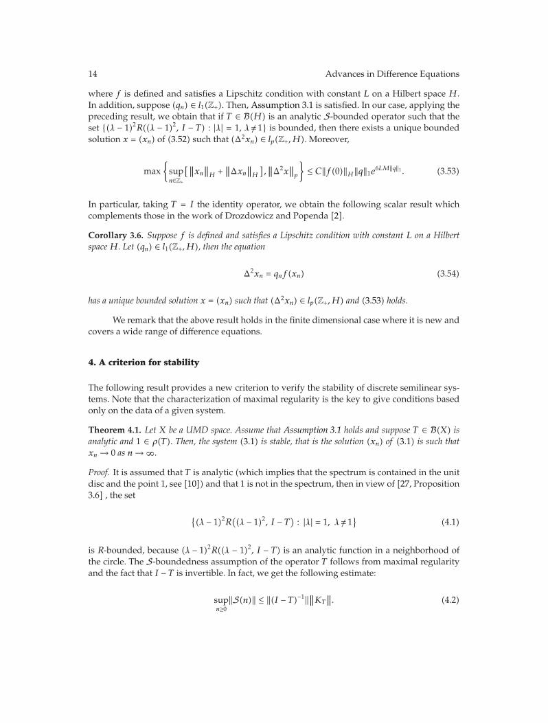
14 Advances in Difference Equations
where f is defined and satisfies a Lipschitz condition with constant L on a Hilbert space H.In addition, suppose (qn) ∈ l1(Z+). Then, Assumption 3.1 is satisfied. In our case, applying thepreceding result, we obtain that if T ∈ B(H) is an analytic S-bounded operator such that theset {(λ − 1)2R((λ − 1)2, I − T) : |λ| = 1, λ /= 1} is bounded, then there exists a unique boundedsolution x = (xn) of (3.52) such that (Δ2xn) ∈ lp(Z+,H). Moreover,
max{supn∈Z+
[ ∥∥xn
∥∥H +∥∥Δxn
∥∥H
],∥∥Δ2x
∥∥p
}≤ C‖f(0)‖H‖q‖1e6LM‖q‖1 . (3.53)
In particular, taking T = I the identity operator, we obtain the following scalar result whichcomplements those in the work of Drozdowicz and Popenda [2].
Corollary 3.6. Suppose f is defined and satisfies a Lipschitz condition with constant L on a HilbertspaceH. Let (qn) ∈ l1(Z+,H), then the equation
Δ2xn = qnf(xn) (3.54)
has a unique bounded solution x = (xn) such that (Δ2xn) ∈ lp(Z+,H) and (3.53) holds.
We remark that the above result holds in the finite dimensional case where it is new andcovers a wide range of difference equations.
4. A criterion for stability
The following result provides a new criterion to verify the stability of discrete semilinear sys-tems. Note that the characterization of maximal regularity is the key to give conditions basedonly on the data of a given system.
Theorem 4.1. Let X be a UMD space. Assume that Assumption 3.1 holds and suppose T ∈ B(X) isanalytic and 1 ∈ ρ(T). Then, the system (3.1) is stable, that is the solution (xn) of (3.1) is such thatxn → 0 as n → ∞.
Proof. It is assumed that T is analytic (which implies that the spectrum is contained in the unitdisc and the point 1, see [10]) and that 1 is not in the spectrum, then in view of [27, Proposition3.6] , the set
{(λ − 1)2R
((λ − 1)2, I − T
): |λ| = 1, λ /= 1
}(4.1)
is R-bounded, because (λ − 1)2R((λ − 1)2, I − T) is an analytic function in a neighborhood ofthe circle. The S-boundedness assumption of the operator T follows from maximal regularityand the fact that I − T is invertible. In fact, we get the following estimate:
supn≥0
‖S(n)‖ ≤ ‖(I − T)−1‖∥∥KT
∥∥. (4.2)

C. Cuevas and C. Lizama 15
By Corollary 3.4, there exists a unique bounded solution xn of (3.1) such that (Δ2xn) ∈lp(Z+, X). Then, Δ2xn → 0 as n → ∞. Next, observe that Assumption 3.1 and estimate (3.10)imply
∥∥f(n, xn,Δxn
)∥∥X ≤∥∥f(n, xn,Δxn
)− f(n, 0, 0)
∥∥X +∥∥f(n, 0, 0)
∥∥X
≤ αn
∥∥(xn,Δxn
)∥∥X×X +
∥∥f(n, 0, 0)∥∥X
≤ αnsupn∈Z+
∥∥(xn,Δxn
)∥∥X×X +
∥∥f(n, 0, 0)∥∥X
≤ 3αn
∥∥x∥∥∞ +∥∥f(n, 0, 0)
∥∥X.
(4.3)
Since (f(·, 0, 0)) ∈ l1(Z+, X) and (αn) ∈ l1(Z+), we obtain that f(n, xn,Δxn) → 0 as n → ∞.Then, the result follows from the fact that 1 ∈ ρ(T) and (3.1).
From the point of view of applications, we specialize to Hilbert spaces. The followingcorollary provides easy-to-check conditions for stability.
Corollary 4.2. Let H be a Hilbert space. Let T ∈ B(H) such that ‖T‖ < 1. Suppose thatAssumption 3.1 holds inH. Then, the system (3.1) is stable.
Proof. First, we note that each Hilbert space is UMD, and then the concept of R-boundednessand boundedness coincide; see [7]. Since ‖T‖ < 1, we get that T is analytic and 1 ∈ ρ(T).Furthermore, for |λ| = 1, λ /= 1, the inequality
∥∥(λ − 1)2R((λ − 1)2, I − T
)∥∥ =
∥∥∥∥∥(λ − 1)2
λ(λ − 2)
∞∑
n=0
(T
λ(λ − 2)
)n∥∥∥∥∥ ≤ |λ − 1|2
|λ − 2| − ‖T‖ ≤ 41 − ‖T‖ (4.4)
shows that the set (4.1) is bounded .
Of course, the same result holds in the finite dimensional case.
5. Local perturbations
In the process of obtaining our next result, we will require the following assumption.
Assumption 5.1. The following conditions hold.
(i)∗ The function f(n, z) is locally Lipschitz with respect to z ∈ X × X; that is for eachpositive number R, for all n ∈ Z+, and z,w ∈ X ×X, ‖z‖X×X ≤ R, ‖w‖X×X ≤ R
‖f(n, z) − f(n,w)‖X ≤ l(n,R)‖z −w‖X×X, (5.1)
where � : Z+ × [0,∞) → [0,∞) is a nondecreasing function with respect to the secondvariable.
(ii)∗ There is a positive number a such that∑∞
n=0�(n, a) < +∞.
(iii)∗ f(·, 0, 0) ∈ �1(Z+, X).

16 Advances in Difference Equations
We need to introduce some basic notations. We denote by W2,pm the Banach space of all
sequences V = (Vn) belonging to �∞(Z+, X), such that Vn = 0 if 0 ≤ n ≤ m, and Δ2V ∈ �p(Z+, X)equipped with the norm
∣∣∣∣∣∣ ·∣∣∣∣∣∣. For λ > 0, denote by W2,p
m [λ] the ball∣∣∣∣∣∣V∣∣∣∣∣∣ ≤ λ in W2,p
m . Ourmain result in this section is the following local version of Theorem 3.3.
Theorem 5.2. Suppose that the following conditions are satisfied.
(a)∗ Assumption 5.1 holds.
(b)∗ T is an S-bounded operator and it has discrete maximal regularity.
Then, there are a positive constant m ∈ N and a unique bounded solution x = (xn) of (3.1) forn ≥ m such that xn = 0 if 0 ≤ n ≤ m and the sequence (Δ2xn) belongs to �p(Z+, X). Moreover, one has
‖x‖∞ +∥∥Δ2x
∥∥p ≤ a, (5.2)
where a is the constant of condition (ii)∗.
Proof. Let β ∈ (0, 1/3). Using (iii)∗ and (ii)∗, there are n1 and n2 in N such that
(M + 2 +
∥∥KT
∥∥)∞∑
j=n1
∥∥f(j, 0, 0)∥∥X ≤ βa, (5.3)
T := β +(M + 2 +
∥∥KT
∥∥)∞∑
j=n2
�(j, a) <13, (5.4)
whereM := supn∈Z+‖S(n)‖.Let V be a sequence in W2,p
m [a/3], with m = max{n1, n2}. A short argument similar to(3.7) and involving Assumption 5.1 shows that the sequence
gn :=
⎧⎨
⎩0, if 0 ≤ n ≤ m,
f(n, Vn,ΔVn), if n > m,(5.5)
belongs to �p. By the discrete maximal regularity, the Cauchy problem (3.12) with gn definedas in (5.5) has a unique solution (zn) such that (Δ2zn) ∈ lp(Z+, X), which is given by
zn = [KV )]n =
⎧⎪⎪⎨
⎪⎪⎩
0, if 0 ≤ n ≤ m,
n−1−m∑
k=0
S(k)f(n − 1 − k, Vn−1−k,ΔVn−1−k), if n ≥ m + 1.(5.6)
We will prove that KV belongs toW2,pm [a/3]. In fact, since
∥∥(Vj,ΔVj
)∥∥X×X ≤ 3‖|V |‖∞ ≤ 3‖|V |‖ < a, (5.7)
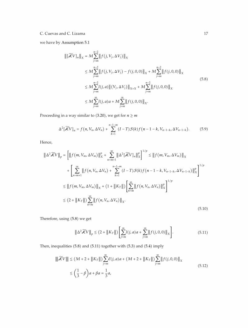
C. Cuevas and C. Lizama 17
we have by Assumption 5.1
∥∥[KV ]n∥∥X = M
n−2∑
j=m
∥∥f(j, Vj ,ΔVj
)∥∥X
≤ Mn−2∑
j=m
∥∥f(j, Vj ,ΔVj
)− f(j, 0, 0)
∥∥X +M
n−2∑
j=m
∥∥f(j, 0, 0)∥∥X
≤ Mn−2∑
j=m
l(j, a)∥∥(Vj,ΔVj
)∥∥X×X +M
n−2∑
j=m
∥∥f(j, 0, 0)∥∥X
≤ M∞∑
j=m
l(j, a)a +M∞∑
j=m
∥∥f(j, 0, 0)∥∥X.
(5.8)
Proceeding in a way similar to (3.20), we get for n ≥ m
Δ2[KV ]n = f(n, Vn,ΔVn
)+
n−1−m∑
k=1
(I − T)S(k)f(n − 1 − k, Vn−1−k,ΔVn−1−k
). (5.9)
Hence,
∥∥Δ2KV∥∥p =[∥∥f(m,Vm,ΔVm
)∥∥pX +
∞∑
n=m+1
∥∥Δ2[KV ]n∥∥pX
]1/p≤∥∥f(m,Vm,ΔVm
)∥∥X
+
[∞∑
n=m+1
∥∥f(n, Vn,ΔVn
)+
n−1−m∑
k=1
(I − T)S(k)f(n − 1 − k, Vn−1−k,ΔVn−1−k
)∥∥pX
]1/p
≤∥∥f(m,Vm,ΔVm
)∥∥X +(1 +∥∥KT
∥∥)[
∞∑
n=m
∥∥f(n, Vn,ΔVn
)∥∥pX
]1/p
≤(2 +∥∥KT
∥∥)∞∑
n=m
∥∥f(n, Vn,ΔVn
)∥∥X.
(5.10)
Therefore, using (5.8) we get
∥∥Δ2KV∥∥p ≤(2 +∥∥KT
∥∥)[
∞∑
j=m
l(j, a)a +∞∑
j=m
∥∥f(j, 0, 0)∥∥X
]. (5.11)
Then, inequalities (5.8) and (5.11) together with (5.3) and (5.4) imply
∣∣∣∣∣∣KV∣∣∣∣∣∣ ≤
(M + 2 +
∥∥KT
∥∥)∞∑
j=m
�(j, a)a +(M + 2 +
∥∥KT
∥∥)∞∑
j=m
∥∥f(j, 0, 0)∥∥X
≤(13− β
)a + βa =
13a,
(5.12)

18 Advances in Difference Equations
proving that KV belongs to W2,pm [a/3]. In an essentially similar way to the proof of
Theorem 3.3, for all V andW inW2,pm [a/3], we prove that
‖KV − KW‖∞ ≤ 3M∞∑
j=m
�(j, a)∣∣∣∣∣∣V −W
∣∣∣∣∣∣, (5.13)
∥∥Δ2KV −Δ2KW∥∥p ≤ 3
(1 +∥∥KT
∥∥)∞∑
j=m
�(j, a)∣∣∣∣∣∣V −W
∣∣∣∣∣∣, (5.14)
whence
∣∣∣∣∣∣KV − KW∣∣∣∣∣∣ ≤ 3
(M + 1 +
∥∥KT
∥∥)∞∑
j=m
�(j, a)∣∣∣∣∣∣V −W
∣∣∣∣∣∣ = 3(T − β)∣∣∣∣∣∣V −W
∣∣∣∣∣∣. (5.15)
Since 3(T − β) < 1, K is a 3(T − β)-contraction. This completes the proof of the theorem.
This enables us to prove, as an application, the following corollary.
Corollary 5.3. Let Bi : X × X → X, i = 1, 2, be two bounded bilinear operators, y ∈ �1(Z+, X),and α, β ∈ �1(Z+,R). In addition, suppose that T is a S-bounded operator and has discrete maximalregularity. Then, there is a unique bounded solution x such that (Δ2x) ∈ lp(Z+, X) for the equation
xn+2 − 2xn+1 + Txn = yn + αnB1(xn, xn
)+ βnB2
(Δxn,Δxn
). (5.16)
Proof. Take l(n,R) := 2R(|αn| + |βn|)(‖B1‖ + ‖B2‖). Then,∑∞
n=0�(n, 1) < +∞. Note also thatf(n, 0, 0) = yn belongs to �1(Z+, X). Hence, Assumption 5.1 is satisfied.
Remark 5.4. We observe that under the hypotheses of the above local theorem and corollary,the same type of conclusions on stability of solutions proved in Section 4 remains true.
Acknowledgments
The authors would like to thank the referees for the careful reading of the manuscript andtheir many useful comments and suggestions. The first author is partially supported byCNPq/Brazil under Grant no. 300068/2005-0. The second author is partially financed byProyecto Anillo ACT-13 and CNPq/Brazil under Grant no. 300702/2007-08.
References
[1] R. P. Agarwal, Difference Equations and Inequalities, vol. 155 of Monographs and Textbooks in Pure andApplied Mathematics, Marcel Dekker, New York, NY, USA, 1992.
[2] A. Drozdowicz and J. Popenda, “Asymptotic behavior of the solutions of the second order differenceequation,” Proceedings of the American Mathematical Society, vol. 99, no. 1, pp. 135–140, 1987.
[3] S. Elaydi, An Introduction to Difference Equations, Undergraduate Texts in Mathematics, Springer, NewYork, NY, USA, 3rd edition, 2005.
[4] V. B. Kolmanovskii, E. Castellanos-Velasco, and J. A. Torres-Munoz, “A survey: stability and bound-edness of Volterra difference equations,” Nonlinear Analysis: Theory, Methods & Applications, vol. 53,no. 7-8, pp. 861–928, 2003.
[5] J. P. LaSalle, The Stability and Control of Discrete Processes, vol. 62 of Applied Mathematical Sciences,Springer, New York, NY, USA, 1986.
C. Cuevas and C. Lizama 19
[6] H. Amann, “Quasilinear parabolic functional evolution equations,” in Recent Avdances in Elliptic andParabolic Issues, M. Chipot and H. Ninomiya, Eds., pp. 19–44, World Scientific, River Edge, NJ, USA,2006.
[7] R. Denk, M. Hieber, and J. Pruss, “R-boundedness, Fourier multipliers and problems of elliptic andparabolic type,”Memoirs of the American Mathematical Society, vol. 166, no. 788, p. 114, 2003.
[8] Ph. Clement, S.-O. Londen, and G. Simonett, “Quasilinear evolutionary equations and continuousinterpolation spaces,” Journal of Differential Equations, vol. 196, no. 2, pp. 418–447, 2004.
[9] W. Arendt, “Semigroups and evolution equations: functional calculus, regularity and kernel esti-mates,” in Evolutionary Equations, vol. 1 of Handbook of Differential Equations, pp. 1–85, North-Holland,Amsterdam, The Netherlands, 2004.
[10] S. Blunck, “Maximal regularity of discrete and continuous time evolution equations,” Studia Mathe-matica, vol. 146, no. 2, pp. 157–176, 2001.
[11] S. Blunck, “Analyticity and discrete maximal regularity on Lp-spaces,” Journal of Functional Analysis,vol. 183, no. 1, pp. 211–230, 2001.
[12] P. Portal, “Discrete time analytic semigroups and the geometry of Banach spaces,” Semigroup Forum,vol. 67, no. 1, pp. 125–144, 2003.
[13] P. Portal, “Maximal regularity of evolution equations on discrete time scales,” Journal of MathematicalAnalysis and Applications, vol. 304, no. 1, pp. 1–12, 2005.
[14] D. Guidetti and S. Piskarev, “Stability of the Crank-Nicolson scheme and maximal regularity forparabolic equations in Cθ(Ω) spaces,” Numerical Functional Analysis and Optimization, vol. 20, no. 3-4, pp. 251–277, 1999.
[15] M. Geissert, “Maximal Lp regularity for parabolic difference equations,” Mathematische Nachrichten,vol. 279, no. 16, pp. 1787–1796, 2006.
[16] C. Cuevas and C. Lizama, “Maximal regularity of discrete second order Cauchy problems in Banachspaces,” Journal of Difference Equations and Applications, vol. 13, no. 12, pp. 1129–1138, 2007.
[17] N. J. Kalton and P. Portal, “Remarks on l1 and l∞ maximal regularity for power bounded operators,”preprint.
[18] J. Popenda, “Gronwall type inequalities,” Zeitschrift fur Angewandte Mathematik und Mechanik, vol. 75,no. 9, pp. 669–677, 1995.
[19] E. Magnucka-Blandzi, J. Popenda, and R. P. Agarwal, “Best possible Gronwall inequalities,” Mathe-matical and Computer Modelling, vol. 26, no. 3, pp. 1–8, 1997.
[20] W. Arendt and S. Bu, “The operator-valued Marcinkiewicz multiplier theorem and maximal regular-ity,”Mathematische Zeitschrift, vol. 240, no. 2, pp. 311–343, 2002.
[21] M. Girardi and L. Weis, “Operator-valued Fourier multiplier theorems on Besov spaces,”Mathematis-che Nachrichten, vol. 251, no. 1, pp. 34–51, 2003.
[22] Ph. Clement, B. de Pagter, F. A. Sukochev, and H. Witvliet, “Schauder decomposition and multipliertheorems,” Studia Mathematica, vol. 138, no. 2, pp. 135–163, 2000.
[23] J. Bourgain, “Some remarks on Banach spaces in which martingale difference sequences are uncondi-tional,” Arkiv for Matematik, vol. 21, no. 1, pp. 163–168, 1983.
[24] D. L. Burkholder, “A geometric condition that implies the existence of certain singular integrals ofBanach-space-valued functions,” in Conference on Harmonic Analysis in Honour of Antoni Zygmund, Vol.I, II (Chicago, Ill., 1981), W. Becker, A. P. Calderon, R. Fefferman, and P. W. Jones, Eds., WadsworthMathematics Series, pp. 270–286, Wadsworth, Belmont, Calif, USA, 1983.
[25] N. Dungey, “A note on time regularity for discrete time heat kernels,” Semigroup Forum, vol. 72, no. 3,pp. 404–410, 2006.
[26] Ph. Clement and G. Da Prato, “Existence and regularity results for an integral equation with infinitedelay in a Banach space,” Integral Equations and Operator Theory, vol. 11, no. 4, pp. 480–500, 1988.
[27] L. Weis, “Operator-valued Fourier multiplier theorems and maximal Lp-regularity,” MathematischeAnnalen, vol. 319, no. 4, pp. 735–758, 2001.
[28] L. Weis, “A new approach to maximal Lp-regularity,” in Evolution Equations and Their Applications inPhysical and Life Sciences, vol. 215 of Lecture Notes in Pure and Applied Mathematics, pp. 195–214, MarcelDekker, New York, NY, USA, 2001.
[29] W. Arendt and S. Bu, “Operator-valued Fourier multipliers on periodic Besov spaces and applica-tions,” Proceedings of the Edinburgh Mathematical Society, vol. 47, no. 1, pp. 15–33, 2004.

20 Advances in Difference Equations
[30] V. Keyantuo and C. Lizama, “Maximal regularity for a class of integro-differential equations withinfinite delay in Banach spaces,” Studia Mathematica, vol. 168, no. 1, pp. 25–50, 2005.
[31] V. Keyantuo and C. Lizama, “Fourier multipliers and integro-differential equations in Banach spaces,”Journal of the London Mathematical Society, vol. 69, no. 3, pp. 737–750, 2004.
[32] V. Keyantuo and C. Lizama, “Periodic solutions of second order differential equations in Banachspaces,”Mathematische Zeitschrift, vol. 253, no. 3, pp. 489–514, 2006.
[33] C. Cuevas and M. Pinto, “Asymptotic properties of solutions to nonautonomous Volterra differencesystems with infinite delay,” Computers & Mathematics with Applications, vol. 42, no. 3–5, pp. 671–685,2001.
[34] C. Cuevas and L. Del Campo, “An asymptotic theory for retarded functional difference equations,”Computers & Mathematics with Applications, vol. 49, no. 5-6, pp. 841–855, 2005.