Quantification of regularity in RR-interval time series using ...
121
New Jersey Institute of Technology Digital Commons @ NJIT eses eses and Dissertations Summer 2005 Quantification of regularity in RR-interval time series using approximate entropy, sample entropy, and multi-scale entropy Nirvish Shah New Jersey Institute of Technology Follow this and additional works at: hps://digitalcommons.njit.edu/theses Part of the Biomedical Engineering and Bioengineering Commons is esis is brought to you for free and open access by the eses and Dissertations at Digital Commons @ NJIT. It has been accepted for inclusion in eses by an authorized administrator of Digital Commons @ NJIT. For more information, please contact [email protected]. Recommended Citation Shah, Nirvish, "Quantification of regularity in RR-interval time series using approximate entropy, sample entropy, and multi-scale entropy" (2005). eses. 511. hps://digitalcommons.njit.edu/theses/511
-
Upload
khangminh22 -
Category
Documents
-
view
3 -
download
0
Transcript of Quantification of regularity in RR-interval time series using ...
New Jersey Institute of TechnologyDigital Commons @ NJIT
Theses Theses and Dissertations
Summer 2005
Quantification of regularity in RR-interval timeseries using approximate entropy, sample entropy,and multi-scale entropyNirvish ShahNew Jersey Institute of Technology
Follow this and additional works at: https://digitalcommons.njit.edu/theses
Part of the Biomedical Engineering and Bioengineering Commons
This Thesis is brought to you for free and open access by the Theses and Dissertations at Digital Commons @ NJIT. It has been accepted for inclusionin Theses by an authorized administrator of Digital Commons @ NJIT. For more information, please contact [email protected].
Recommended CitationShah, Nirvish, "Quantification of regularity in RR-interval time series using approximate entropy, sample entropy, and multi-scaleentropy" (2005). Theses. 511.https://digitalcommons.njit.edu/theses/511

Copyright Warning & Restrictions
The copyright law of the United States (Title 17, United States Code) governs the making of photocopies or other
reproductions of copyrighted material.
Under certain conditions specified in the law, libraries and archives are authorized to furnish a photocopy or other
reproduction. One of these specified conditions is that the photocopy or reproduction is not to be “used for any
purpose other than private study, scholarship, or research.” If a, user makes a request for, or later uses, a photocopy or reproduction for purposes in excess of “fair use” that user
may be liable for copyright infringement,
This institution reserves the right to refuse to accept a copying order if, in its judgment, fulfillment of the order
would involve violation of copyright law.
Please Note: The author retains the copyright while the New Jersey Institute of Technology reserves the right to
distribute this thesis or dissertation
Printing note: If you do not wish to print this page, then select “Pages from: first page # to: last page #” on the print dialog screen

The Van Houten library has removed some ofthe personal information and all signatures fromthe approval page and biographical sketches oftheses and dissertations in order to protect theidentity of NJIT graduates and faculty.

ABSTRACT
QUANTIFICATION OF REGULARITY IN RR-INTERVAL TIME SERIESUSING APPROXIMATE ENTROPY, SAMPLE ENTROPY,
AND MULTI-SCALE ENTROPY
byNirvish Shah
Heart rate variability (HRV) has proven to be a useful noninvasive tool to study the
neuronal control of the heart. Recently, nonlinear dynamic methods based on chaos
theory and fractal dynamics have been developed to uncover the nonlinear fluctuations in
heart rate. Approximate Entropy (ApEn), Sample Entropy (SampEn) and Multi-scale
Entropy (MSE) are measures based on chaos theory that quantify the regularity in time
series. This study has been designed to examine the ability of these measures to
distinguish the RR-interval time series of normal subjects (NSR) from subjects with
congestive heart failure (CHF). The study was conducted on the RR-interval data of 44
NSR subjects and 18 CHF subjects. In addition to this, entropy measures of three
apparently healthy subjects were calculated during sitting, standing, exercise and paced
breathing to determine the change in entropy measures during these conditions. The
results showed that ApEn and SampEn measures for 1000 RR-intervals were
significantly (P < 0.005) higher for the NSR group than the CHF group. However, no
significant difference was observed for these measures calculated for 40,000 RR-
intervals. MSE analysis revealed that the complexity of the RR-interval time series was
significantly higher for the NSR group than the CHF group at all scales but one. SampEn
was significantly lower during exercise while there was no significant difference in
SampEn for other activities. The results reproduced the findings of others. This study
suggests a general decrease in entropy in subjects with congestive heart failure.

QUANTIFICATION OF REGULARITY IN RR-INTERVAL TIME SERIESUSING APPROXIMATE ENTROPY, SAMPLE ENTROPY,
AND MULTI-SCALE ENTROPY
ByNirvish Shah
A ThesisSubmitted to the Faculty of
New Jersey Institute of Technologyin Partial Fulfillment of the Requirements for the Degree of
Master of Science in Biomedical Engineering
Department of Biomedical Engineering
August 2005


APPROVAL PAGE
QUANTIFICATION OF REGULARITY IN RR-INTERVAL TIME SERIESUSING APPROXIMATE ENTROPY, SAMPLE ENTROPY,
AND MULTI-SCALE ENTROPY
Nirvish Shah
Dr. Stanley Reisman, Thesis Advisor DateProfessor of Biomedical Engineering, NJIT
Dr. Ronald Rockland, Committee Member DateAssociate Professor of Engineering Technology, NJIT
Dr Tara Alvarez, Comm* Member DateAssistant Professor of Biomedical Engineering, NJIT

BIOGRAPHICAL SKETCH
Author: Nirvish S. Shah
Degree: Master of Science
Date: August 2005
Graduate and Undergraduate Education:
■ Master of Science in Biomedical EngineeringNew Jersey Institute of Technology, Newark, New Jersey, 2005
■ Bachelor of Science in Biomedical and Instrumentation EngineeringC.U.Shah College of Engineering and Technology, Wadhwan, India, 2003
Major: Biomedical Engineering
iv

ACKNOWLEDGMENT
I would like to thank my thesis advisor Dr. Stanley Reisman for his invaluable guidance.
It was his direction that immensely contributed to the successful completion of this thesis.
I would also like to thank Dr. Ronald Rockland and Dr. Tara Alvarez for serving as
members of my thesis committee.
I would like to thank the pioneers of PhysioNet for providing a large database of
complex physiologic signals and a large library of software for physiologic signal
processing and analysis on Internet.
I would like to thank my colleagues at the Biomedical Signal Processing
Laboratory at NJIT for their help. I would also like to thank my friends for being subjects
in my research.
I would like to thank my parents for their moral and financial support without
which my study at NJIT would not have been possible. I would also like to thank my
maternal grandfather for lending me a helping hand.
Above all, I would like to thank God for His guardianship.
v

TABLE OF CONTENTS
Chapter Page
1 INTRODUCTION 1
1.1 Overview 1
1.2 Outline of the thesis 4
2 PHYSIOLOGICAL AND ENGINEERING BACKGROUND 5
2.1 Physiological Background 5
2.1.1 The Cardiovascular System 5
2.1.2 The Autonomic Nervous System 9
2.1.3 The Electrocardiogram 12
2.1.4 Heart Rate Variability 13
2.2 Engineering Background 17
2.2.1 Introduction 17
2.2.2 Nonlinear Dynamics and Chaos 17
2.2.3 Analytic Techniques to Detect Nonlinear Dynamics Behavior 24
2.2.4 Heart Rate and Nonlinear Dynamics 29
3 METHODS 30
3.1 Approximate Entropy 30
3.1.1 Algorithm 30
3.1.2 Implementation 33
3.1.3 Interpretation 36
3.1.4 Relationship with other Approaches 41
vi

TABLE OF CONTENTS(Continued)
Chapter Page
3.1.5 Advantages and Disadvantages 45
3.2 Sample Entropy 47
3.2.1 Algorithm 47
3.2.2 Implementation 49
3.2.3 Interpretation 52
3.2.4 Comparison with ApEn 52
3.2.5 Advantages and Disadvantages 56
3.3 Multi-Scale Entropy 57
3.3.1 Algorithm 58
3.3.2 Implementation 59
3.3.3 Interpretation 60
4 DATA ACQUISITION AND ANALYSIS 62
4.1 Data Acquisition 62
4.2 Data. Anomalies and Correction 63
4.3 Programs for Data Analysis 64
4.4 Results of Data Analysis 64
4.5 t-Test Analysis 80
4.6 ANOVA Analysis 84
4.7 MSE Analysis 89
5 CONCLUSIONS AND FUTURE WORK 91
5.1 Conclusions and Future Work 91
vii

TABLE OF CONTENTS(Continued)
Chapter Page
APPENDIX A Henon Attractor 95
APPENDIX B Programs for the Study 96
REFERENCES 103
viii

LIST OF TABLES
Table Page
3.1 ApEn(2,R,N) Calculations for Two Deterministic Models 34
3.2 SampEn(2,R,N) Calculations for Two Deterministic Models 51
4.1 ApEn(2,0.2,N) vs. Data Lengths for NSR Subjects 66
4.2 ApEn(2,0.2,1000) vs. Consecutive Data Points for NSR Subjects 67
4.3 ApEn(2,0.2,N) vs. Data Lengths for CHF Subjects 68
4.4 ApEn(2,0.2,1000) vs. Consecutive Data Points for CHF Subjects 68
4.5 SampEn(2,0.2,N) vs. Data Lengths for NSR Subjects 70
4.6 SampEn(2,0.2,1000) vs. Consecutive Data Points for NSR Subjects 71
4.7 SampEn(2,0.2,N) vs. Data Lengths for CHF Subjects 72
4.8 SampEn(2,0.2,1000) vs. Consecutive Data Points for CHF Subjects 72
4.9 MSE Analysis for NSR Subjects 74
4.10 MSE Analysis for CHF Subjects 76
4.11 t-Test for ApEn(2,0.2,1000) for NSR and CHF Subjects 80
4.12 t-Test for ApEn(2,0.2,40000) for NSR and CHF Subjects. 81
4.13 t-Test for SampEn(2,0.2,1000) for NSR and CHF Subjects 82
4.14 t-Test for SampEn(2,0.2,40000) for NSR and CHF Subjects 83
4.15 SampEn(2,0.2,1000) for Different Activities 85
4.16 Two-Factor ANOVA to Find the Effect of Activities on SampEn 85
4.17 ANOVA for Sitting vs. Standing Activity 86
4.18 ANOVA for Sitting vs. Paced Breathing Activity 86
ix

LIST OF TABLES(Continued)
Table Page
4.19 ANOVA for Sitting vs. Exercise Activity 87
4.20 ANOVA for Standing vs. Paced Breathing Activity 87
4.21 ANOVA for Standing vs. Exercise Activity 88
4.22 ANOVA for Paced Breathing vs. Exercise Activity 88
4.23 t-Test for MSE for NSR and CHF Subjects 90

LIST OF FIGURES
Figure Page
1.1 Heart rate time series 2
2.1 The Human Heart 5
2.2 The Circulatory System 7
2.3 The Conduction System 8
2.4 The Autonomic Nervous System 11
2.5 The Electrocardiogram 12
2.6 x(n) vs. x(n+1) for the Logistic equation 19
2.7 Iterative solutions of the Logistic equation for different values of r 20
2.8 Bifurcation diagram for the Logistic equation 21
2.9 Sensitive dependence on initial conditions 22
2.10 Phase plane and Return maps of periodic, chaotic and random signals 26
3.1 ApEn(2,0.2,N) vs. N for Logistic equation 35
3.2 ApEn(2,0.2,N) vs. N for Henon attractor 36
3.3 x(n) vs. N for R = 1.25 in the Logistic equation 37
3.4 x(n) vs. N for R = 3.20 in the Logistic equation 38
3.5 x(n) vs. N for R = 3.54 in the Logistic equation 38
3.6 x(n) vs. N for R = 3.99 in the Logistic equation 39
3.7 x(n) vs. N for random signal 39
3.8 Amplitude vs. Time for MIX(P) p=0.1, 0.4 and 0.9 43
3.9 SampEn(2,0.2,N) vs. N for Logistic equation 50
xi

LIST OF FIGURES(Continued)
Figure Page
3.10 SampEn(2,0.2,N) vs. N for Henon attractor 51
3.11 ApEn, SampEn vs. N for uniform i.i.d. random variables 53
3.12 ApEn, SampEn vs. r for uniform i.i.d. random variables 54
3.13 ApEn(2,0.2,100), SampEn(2,0.2,100) vs. r for uniform i.i.d. randomvariables 54
3.14 ApEn(2,0.2,5000), SampEn(2,0.2,5000) vs. r for uniform i.i.d. randomvariables 55
3.15 ApEn(2,0.2,20000), SampEn(2,0.2,20000) vs. r for uniform i.i.d. randomvariables 55
3.16 Schematic illustration of the coarse-graining procedure for scale 2 and 3 59
3.17 MSE analysis of white noise and 1/f noise 61
4.1 SampEn(m,r,1000) vs. r for different r for NSR group.. 77
4.2 SampEn(m,r,1000) vs. m for different r for NSR group 78
4.3 ApEn(2,0.2,1000) vs Consecutive data points for NSR group 79
4.4 SampEn(2,0.2,1000) vs Consecutive data points for NSR group 79
4.5 ApEn(2,0.2,N) vs. Data Lengths for NSR and CHF groups 81
4.6 SampEn((2,0.2,N) vs. Data Lengths for NSR and CHF groups 83
4.7 MSE Analyses for NSR and CHF groups 90
A.1 Henon Attractor 95
xii

CHAPTER 1
INTRODUCTION
1.1 Overview
Biological systems are complex systems. They are systems that are spatially and
temporally complex, built from a dynamic web of interconnected feedback loops marked
by interdependence, pleiotropy and redundancy [1]. Complex systems have the properties
that cannot wholly be understood by understanding parts of the system. The properties of
the system are distinct from the properties of the parts, and they depend on the integrity
of the whole; the systemic properties vanish when the system breaks apart; whereas, the
properties of the parts are maintained [1]. Quantifying the complexity of the physiologic
signals in health and disease has been the focus of considerable attention. Such metrics
have been potentially important applications with respect to evaluating both dynamical
models of biologic control systems and bedside diagnostics [1]. For example, a wide
class of disease states, as well as aging, appears to degrade physiologic information
content and reduce the adaptive capacity of the individual [1]. Loss of complexity,
therefore, has been proposed as a generic feature of pathologic dynamics.
Heart rate variability is one such metric. It refers to the regulation of the SA node
by the sympathetic and parasympathetic branch of the autonomic nervous system. Heart
rate variability has become the conventionally accepted term to describe variations in
both instantaneous heart rate and RR intervals [2]. The clinical relevance of HRV was
first appreciated in 1965 when Hon and Lee noted that fetal distress was preceded by
alterations in interbeat intervals before any appreciable change occurred in heart rate
itself [2]. The clinical importance of HRV became appreciated in the late 1980s, when it
1

2
was confirmed that HRV was a strong and independent predictor of mortality after an
acute myocardial infarction [2]. Statistical time domain methods based on mean and
standard deviation have been used to characterize HRV. Figure 1.1 shows two sequences
of interbeat intervals, one for a normal individual and one for a subject with congestive
heart failure. Visual inspection makes clear the existence of differences in the dynamics
generating the two signals. However, the signals have the same means and standard
deviations. Hence additional methods are required if these two signals are to be
distinguished. [3].
Figure 1.1 Heart rate time series [3].
Spectral analysis assesses HR fluctuations averaged over time and thus provides
only an overall measure of HRV [4]. Whereas this method describes cyclic variations in
heart rate, such as respiratory sinus arrhythmia, autonomic nervous system mechanisms

3
governing beat-to-beat changes may be masked by time averaging [4]. Furthermore,
Guevara and others observed nonlinear behavior in cardiac tissue [5]. Ritzenberg
observed a variety of electro-physiologic and hemodynamic phenomena indicative of
chaotic behavior [5]. Also, the human heart rate was found to exhibit 1/f behavior. This
has led to the development of methods based on fractal dynamics and chaos theory to
characterize the intrinsic nature of HRV. Approximate entropy is one such method based
on chaos theory developed by Pincus et al. for analyzing time series data. It is used to
differentiate among data sets on the basis of pattern regularity in the time series. ApEn
has been extensively used in the evaluation of heart rate dynamics. Heart rate becomes
more orderly with age, exhibiting decreased ApEn [1]. Heart rate ApEn is decreased in
infants with aborted sudden infant death syndrome [1]. Sample Entropy, developed by
Moorman et al. [6], is a refinement of ApEn. Finally, because both ApEn and SampEn
evaluate regularity on one scale only, Goldberger et al. [7] developed multi-scale entropy
to evaluate temporal complexity of the physiologic signal on multiple scales. This study
has been designed to examine these methods.
The goal of this research is to verify the ability of these methods to distinguish
between the RR interval time series derived from normal subjects and subjects with
congestive heart failure. Also a small study has been designed to see the effect of various
activities such as paced breathing and exercise on these entropy measures.

4
1.2 Outline of the Thesis
Chapter 1 summarizes the scope of the research involving the evaluation of various
entropy measures in distinguishing RR interval data sets derived from normal subjects
and subjects with congestive heart failure.
Chapter 2 presents the physiology background for studying human cardiac dynamics and
engineering background for analyzing the RR interval time series.
Chapter 3 presents the detailed description of each of the methods.
Chapter 4 presents the description of the data acquisition, protocols used in the study and
the results of the analysis.
Chapter 5 presents the conclusion of the results obtained in chapter 4 and suggestions for
future work.
CHAPTER 2
PHYSIOLOGICAL AND ENGINEERING BACKGROUND
2.1 Physiological Background
2.1.1 The Cardiovascular System
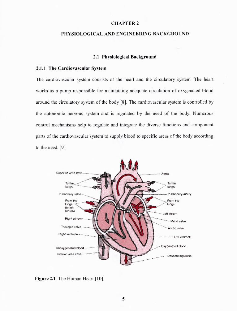
The cardiovascular system consists of the heart and the circulatory system. The heart
works as a pump responsible for maintaining adequate circulation of oxygenated blood
around the circulatory system of the body [8]. The cardiovascular system is controlled by
the autonomic nervous system and is regulated by the need of the body. Numerous
control mechanisms help to regulate and integrate the diverse functions and component
parts of the cardiovascular system to supply blood to specific areas of the body according
to the need. [9].
Figure 2.1 The Human Heart [10].
5

6
The human heart is a hollow, cone-shaped muscle, about the size of a clenched
fist, located obliquely between the lungs and behind the sternum. The apex of the cone
points down and to the left. The heart is encased in a double layer of tissue called the
pericardium. This double layer of tissue helps the heart stay in position and protects it
from harm. The heart (Figure 2.1) is a dual pump, consisting of a two-chambered pump
on both the left and right sides. The upper chambers (the atria) are inputs to the pumps
and the lower chambers (the ventricles) are output of the pumps.
The heart serves as a pump to move blood through vessels called arteries and
veins. Blood is carried away from the heart in arteries and is brought back to the heart in
veins. When blood is circulated through the body, it carries oxygen and nutrients to the
organs and tissues and returns carrying carbon dioxide to be excreted through the lungs
and various waste products to be excreted through the kidneys. The deoxygenated blood
is returned to the right side of the heart via the venous system. Blood returns to the right
atrium of the heart through the superior and inferior vena cava. Blood leaves the right
atrium through the tricuspid valve to enter the right ventricle. From the right ventricle it
passes through the pulmonary semilunar valve to the pulmonary artery. This vessel
carries blood to the lungs, where exchange of gases takes place. Blood from the lungs
reenters the heart through the left atrium. It then passes through the mitral valve to the
left ventricle, and than back into the mainstream of the circulatory system via the aortic
valve. The greater artery attached to the left ventricle is called the aorta. Blood then
circulates through the body to again return to the right side of the heart via the superior
and inferior vena cava. [11].
7
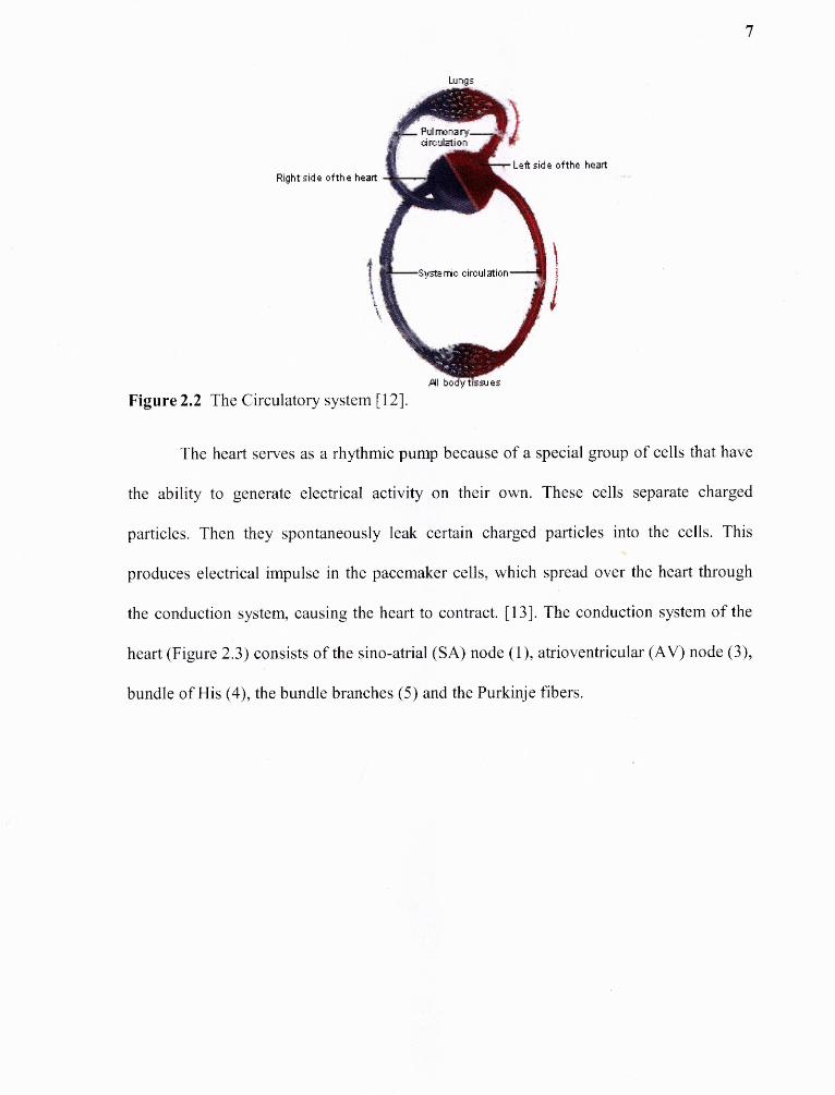
Figure 2.2 The Circulatory system [12].
The heart serves as a rhythmic pump because of a special group of cells that have
the ability to generate electrical activity on their own. These cells separate charged
particles. Then they spontaneously leak certain charged particles into the cells. This
produces electrical impulse in the pacemaker cells, which spread over the heart through
the conduction system, causing the heart to contract. [13]. The conduction system of the
heart (Figure 2.3) consists of the sino-atrial (SA) node (1), atrioventricular (AV) node (3),
bundle of His (4), the bundle branches (5) and the Purkinje fibers.

8
Figure 2.3 The Conduction System [14].
The SA node, located in the top of the right atrium, serves as the natural
pacemaker of the heart. It provides the electrical stimulus triggering the contraction of the
heart muscle. When the SA node discharges a pulse, then electrical stimulus spreads
across the atria, causing them to contract. Blood in the atria is forced into the ventricles.
There is a band of specialized tissue between the SA node and the AV node, which
carries the signal to the AV node. The electrical stimulus then reaches the AV node,
located in the lower part of the wall between the atria near the ventricles. The AV node
provides the only electrical connection between the atria and ventricles; otherwise, the
atria are insulated from the ventricles by tissue that does not conduct electricity. The AV
node delays transmission of the electric stimulus so that the atria can contract completely
and the ventricles can fill with as much blood as possible before the ventricles are
electrically signaled to contract. After passing through the AV node, the electrical

9
stimulus travels down the bundle of His, a group of fibers that divide into a left bundle
branch for the left ventricle and a right bundle branch for the right ventricle. The
electrical stimulus then spreads in a regulated manner over the surface of the ventricles
through Purkinje fibers, from the bottom up, initiating contraction of the ventricles,
which ejects blood from the heart. Any of the electrical tissue in the heart has the ability
to be a pacemaker. However, the SA node generates an electric stimulus faster than the
other tissues so it is normally in control. If the SA node should fail, the other parts of the
electrical system can take over, although usually at a slower rate. [15].
The rate at which the pacemaker discharges the electric stimulus determines the
heart rate. Although the pacemaker cells produce the electrical stimulus that causes the
heart to beat, neurally, chemically and physically induced homeostatic mechanisms
control the rate at which the pacemaker cells fire. The most important extrinsic influences
on heart rate are exerted by the Autonomic Nervous System.
2.1.2 The Autonomic Nervous System
The nervous system is a complex interconnection of nervous tissue that is connected with
the integration and control of all bodily functions. It is generally considered the most
complex bodily system. [16]. It is divided into several major divisions distinguished by
anatomy and physiology including the following:
Central Nervous System (CNS), which is enclosed within the skull and vertebral column
— brain and spinal cord.
Peripheral Nervous System (PNS), which consists of nervous tissue outside the skull and
vertebral column — periphery of the body. Subdivisions of the PNS include:

10
Somatic system, which supplies sensory motor and sensory fibers to the skin and skeletal
muscles.
Autonomic Nervous System (ANS), which supplies motor fibers to smooth muscle,
cardiac muscle, and glands in the body viscera. It functions "automatically" at the reflex
and subconscious levels to keep basic body system operating. Figure 2.4 shows the ANS,
including sympathetic (stimulatory) and parasympathetic (inhibitory) areas. Equilibrium
of the following bodily functions is obtained through the ANS:
1. Heart function — rate and volume output.
2. Blood pressure — arterivenous vessel size.
3. Blood sugar — regulation of liver action.
4. Digestion — regulation of gastric action.
5. Growth — hormone secretion through the endocrine system.
6. Body temperature — sweat glands.
7. Body fluid balance — sweat and kidney functions.
8. Emotional reaction — endocrine system and the brain.
The sympathetic and the parasympathetic nervous systems function as antagonists
to regulate these body systems. [16].

11
Figure 2.4 The Autonomic Nervous System [17].
2.1.2.1 Sympathetic Nervous System (SNS). This system is formed by thoracic
and lumbar nerve outflows. Body resources are made more available through stimulation
by this system. Visceral functions are involved. The main function of the sympathetic
nervous system is to prepare the body for stressful or emergency situations. For example,
a massive sympathetic discharge is associated with the liberation of epinephrine from the
adrenal glands. This increases heart rate and skeletal muscle movements that characterize
the "fight or flight" state. [16].
2.1.2.2 Parasympathetic Nervous System (PSNS). This system arises from
cranial motor nerve outflows from the brain stem and spinal nerves. The main function of
the parasympathetic nervous system is to prepare the body for ordinary situations. For
example, during sleep, this system acts to slow heart rate down to conserve energy. [16].
12
2.1.3 The Electrocardiogram
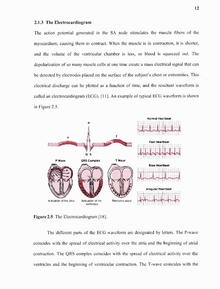
The action potential generated in the SA node stimulates the muscle fibers of the
myocardium, causing them to contract. When the muscle is in contraction, it is shorter,
and the volume of the ventricular chamber is less, so blood is squeezed out. The
depolarization of so many muscle cells at one time create a mass electrical signal that can
be detected by electrodes placed on the surface of the subject's chest or extremities. This
electrical discharge can be plotted as a function of time, and the resultant waveform is
called an electrocardiogram (ECG). [11]. An example of typical ECG waveform is shown
in Figure 2.5.
Figure 2.5 The Electrocardiogram [18].
The different parts of the ECG waveform are designated by letters. The P-wave
coincides with the spread of electrical activity over the atria and the beginning of atrial
contraction. The QRS complex coincides with the spread of electrical activity over the
ventricles and the beginning of ventricular contraction. The T-wave coincides with the

13
recovery phase of the ventricles. The recovery phase of the atria is overshadowed by the
ventricular contraction. The heart rate can be calculated from an electrocardiogram [19].
Heart rate is defined as the number of R waves in one minute, i.e. the number of times the
heart contracts in a minute. The normal heart rate of the human is 72 beats per minute
(i.e. 72 R waves in one minute or one R wave in every 0.83 seconds or the distance
between RR interval is 0.83 seconds); however, it varies from person to person.
According to the classical concepts of physiologic control, healthy systems are
self-regulated to reduce variability and maintain physiologic constancy [20]. That is, it
was believed that parameters like heart rate, blood pressure, etc. show consistency under
resting condition and any variation in them was treated as noise or averaged out [21].
Contrary to the predictions of homeostasis, however, the output of a wide variety of
systems fluctuates in a complex manner, even under resting conditions [20]. The human
ECG, even in case of a resting subject, displays a considerable amount of fluctuations in
time, as well as in amplitude [22]. This phenomenon of fluctuation in the interval
between consecutive heartbeats is called the Heart Rate Variability.
2.1.4 Heart Rate Variability
Beat to beat fluctuation in the heart rate partly reflects the interplay between various
perturbations of cardiovascular fluctuation and the response of the cardiovascular
regulatory systems to these perturbations [16]. The changes in heart rate behavior may be
either exogenous or endogenous. The various factors that influence the heart rate
variability are:

14
1. The Autonomic Nervous System Regulation.
The rate at which the heart beats is determined by two opposing systems — the
sympathetic nervous system (SNS) and the parasympathetic nervous system (PSNS). The
SNS division works through the plexus of nerves that end in the SA node, the AV node
and the myocardium and through the hormone epinephrine and nonepinephrine, which
are released by the adrenal glands and the nerve endings. The PSNS works through the
vagal nerve that innervates the SA node, the AV node and the atrial myocardium. Under
the resting condition, both divisions continuously send impulses to the SA node of the
heart, but the predominant influence is inhibitory. Thus, the heart is said to exhibit vagal
tone, and the heart rate is generally slower than it would be if the vagal nerves were not
stimulated [16]. When either division is stimulated more strongly by sensory inputs
relayed from various parts of the cardiovascular system, the effect of alternate division is
temporarily reduced. Activation of the SNS area results from the emotional or physical
stressors causing the heart rate to increase. Activation of the PSNS area reduces the heart
rate and contractility when the stressful situation has passed. However, the PSNS division
may be persistently activated in certain emotional conditions, such as grief or depression
[16].
2. Chemical Regulation.
Chemicals (ions and hormones) normally present in blood and other bodily fluids
may influence heart rate, particularly if they become excessive or deficient.
i. Hormones: Epinephrine liberated by the adrenal glands during periods of
SNS activation and nonepinephrine released by sympathetic nerves enhances heart rate
15
and contractility. Thyroxin released by thyroid gland causes a slower but more sustained
increase in heart rate when it is released in large quantities.
ii. Ions: Physiologic relationships between intracellular and extracellular ions
must be maintained for normal heart function. Hypocalcaemia depresses the heart.
Hypercalcaemia tightly couples the excitation - contraction mechanism causing an
increase in heart rate. Excessive amount of ionic sodium and potassium lead to heart
blocks. [16].
3. Respiratory Sinus Arrhythmia (RSA).
RSA is heart rate variability in synchrony with respiration, by which the RR
interval is shortened during inspiration and prolonged during expiration. The activity of
the vagus nerve is modulated by respiration, and hence SA node activity is secondarily
modulated by the respiratory rhythm. During inspiration, the activity of the efferent vagal
nerve is almost abolished. Hence, the RR interval is shortened. During expiration, the
activity of the efferent vagal nerve reaches its maximum, thus prolonging the RR interval.
[23].
4. Baroreceptor Reflex Regulation.
Baroreceptors, located in nearly every large artery of the neck and thorax, detect
changes in arterial pressure. When arterial blood pressure rises and stretches these
receptors, they send off a faster stream of impulses to the vasomotor center. This inhibits
the vasomotor center, reducing impulse transmission along the vasomotor fibers, and
results in vasodilatation and a decline in blood pressure. Afferent impulses from the
baroreceptors reach cardiac inhibitory center in the medulla, leading to a reduction in
heart rate and contractility. [16].
16
5. Physical Factors.
A number of physical factors including age, gender, exercise, and body
temperature, influence heart rate. Resting heart rate is fastest in the fetus and gradually
decreases throughout a lifetime. Average heart rate is faster in females than in males.
Exercise promotes increased heart rate by acting through the SNS. Heat increases the
heart rate by increasing metabolic rate of the cardiac cells. [16].
Subtle beat-to-beat fluctuations in cardiovascular signals have received only little
attention until recently, most probably due to a lack of high-resolution
electrocardiographic recordings and digital computers with adequate calculation capacity.
Since the introduction of such computers, computation of heart rate variability has been
possible. [21]. The clinical relevance of HRV was first appreciated in 1965 when Hon
and Lee noted that fetal distress was preceded by alterations in interbeat intervals before
any appreciable change occurred in the heart rate itself. Wolf et al. first showed the
association of higher risks of post-infarction mortality with reduced HRV in 1977. The
clinical importance of HRV became appreciated in the late 1980s, when it was confirmed
that HRV was a strong and independent predictor of mortality after an acute myocardial
infarction. In general higher HRV represents healthy conditions and lower HRV
represents diseased conditions. [2].
HRV analysis has become an important tool in cardiology because it is
noninvasive and provides prognostic information on patients with heart disease [24].
Time and frequency domain measures of heart rate variability are most commonly used
methods of analysis. New methods based on non-linear dynamics have also been
introduced for heart rate variability analysis.

17
2.2 Engineering Background
2.2.1 Introduction
Statistical time domain and frequency domain measures assume that the analyzed
segment of the RR interval time series is stationary or that the variations are harmonic or
sinusoidal. This is, however, not the case in complex biological regulation systems.
Fluctuations in heart rate contain both periodic and non-periodic fluctuations. The non-
periodic fluctuations are not random but arise from dynamics of chaotic nature and are
governed by deterministic laws. Thus in order to get a better understanding of heart rate
regulation, methods based on non-linear mathematics and chaos theory have been
developed. These methods do not attempt to assess the actual magnitude of heart rate
variability but describe the complexity or fractal dynamics of the RR interval time series.
These methods may provide information beyond the conventional time and frequency
domain methods. [25].
Before describing the metrics used to characterize the non-linear dynamics of the
RR interval time series, a brief review of the concepts of nonlinear dynamics and chaos
theory is provided to facilitate the understanding of these measures.
2.2.2 Nonlinear Dynamics and Chaos
The dynamics of any situation refers to how the situation changes with time. A
deterministic dynamical system is a set of rules or equations that describe how variables
change over time. The discrete time dynamical systems theory is an area of mathematics
that studies the applications of difference and differential equations to describe the
behavior of the complex systems. Linear dynamical systems follow the principles of
proportionality and superposition. Proportionality means that the output bears a straight-

18
line relationship with the input. Superposition refers to the fact that the behavior of the
linear system composed of multiple components can be fully understood and predicted by
considering one input at a time and finding their individual input-output relationships
[26]. The overall output is the summation of the outputs resulting from these individual
inputs. In contrast, the nonlinear dynamical systems do not follow the principles of
proportionality and/or superposition. The non-linearity in a dynamical system arises
because the function specifying the change is nonlinear [26]. In nonlinear systems, small
changes can have dramatic and unanticipated effects, as the law of proportionality does
not hold. Also nonlinear systems with multiple inputs cannot be understood by analyzing
these inputs individually because the inputs interact in a nonlinear way. They may exhibit
various kinds of behavior like periodicity, multiple periodicity, and erratic behavior.
Consider the logistic equation:
xn+1 = rxn (1-xn) (2.1)
This simple model is often used to introduce chaos because it displays major chaotic
concepts. The non-linearity of this equation arises from the quadratic term x n2 [26].
Plotting xn+1 vs. xn reveals a nonlinear relation as shown in Figure 2.6.
19
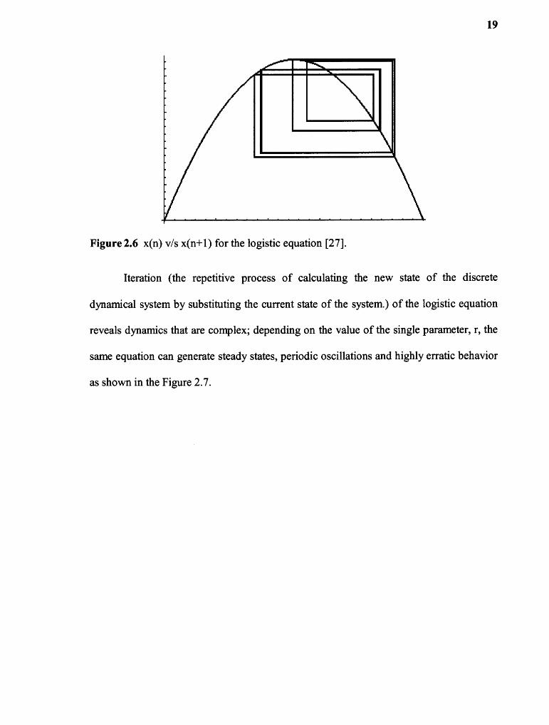
Figure 2.6 x(n) v/s x(n+1) for the logistic equation [27].
Iteration (the repetitive process of calculating the new state of the discrete
dynamical system by substituting the current state of the system.) of the logistic equation
reveals dynamics that are complex; depending on the value of the single parameter, r, the
same equation can generate steady states, periodic oscillations and highly erratic behavior
as shown in the Figure 2.7.
20
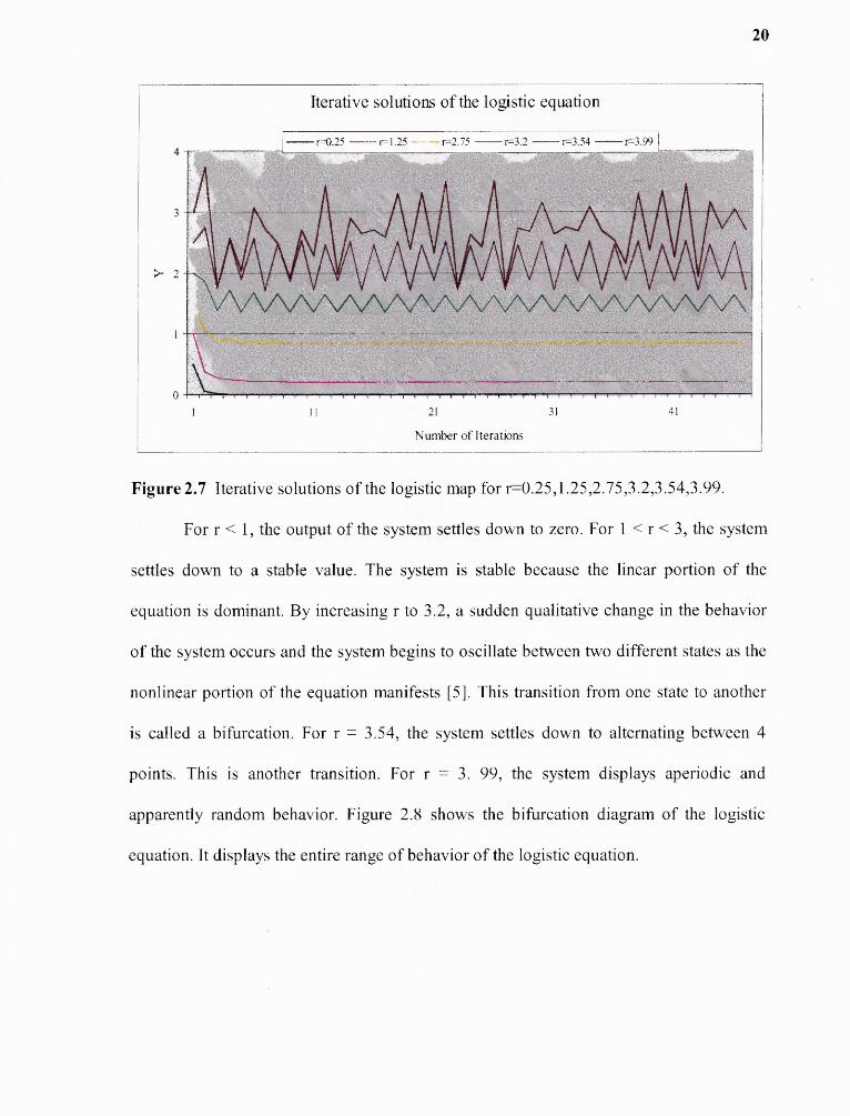
Figure 2.7 Iterative solutions of the logistic map for r=0.25,1.25,2.75,3.2,3.54,3.99.
For r < 1, the output of the system settles down to zero. For 1 < r < 3, the system
settles down to a stable value. The system is stable because the linear portion of the
equation is dominant. By increasing r to 3.2, a sudden qualitative change in the behavior
of the system occurs and the system begins to oscillate between two different states as the
nonlinear portion of the equation manifests [5]. This transition from one state to another
is called a bifurcation. For r = 3.54, the system settles down to alternating between 4
points. This is another transition. For r = 3. 99, the system displays aperiodic and
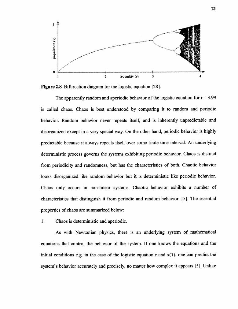
apparently random behavior. Figure 2.8 shows the bifurcation diagram of the logistic
equation. It displays the entire range of behavior of the logistic equation.
21
Figure 2.8 Bifurcation diagram for the logistic equation [28].
The apparently random and aperiodic behavior of the logistic equation for r = 3.99
is called chaos. Chaos is best understood by comparing it to random and periodic
behavior. Random behavior never repeats itself, and is inherently unpredictable and
disorganized except in a very special way. On the other hand, periodic behavior is highly
predictable because it always repeats itself over some finite time interval. An underlying
deterministic process governs the systems exhibiting periodic behavior. Chaos is distinct
from periodicity and randomness, but has the characteristics of both. Chaotic behavior
looks disorganized like random behavior but it is deterministic like periodic behavior.
Chaos only occurs in non-linear systems. Chaotic behavior exhibits a number of
characteristics that distinguish it from periodic and random behavior. [5]. The essential
properties of chaos are summarized below:
1. Chaos is deterministic and aperiodic.
As with Newtonian physics, there is an underlying system of mathematical
equations that control the behavior of the system. If one knows the equations and the
initial conditions e.g. in the case of the logistic equation r and x(1), one can predict the
system's behavior accurately and precisely, no matter how complex it appears [5]. Unlike

22
Newtonian physics, however, chaotic behavior never repeats itself exactly [5]. There are
no cycles that recur at regular interval.
2. Chaotic system is sensitive to initial conditions.
This means that very small difference in initial conditions will result in large
differences in behavior at a later point in time. For example, Figure 2.9 shows the
behavior of the logistic equation for x(1) = 0.5 and 0.5001. The two behaviors are almost
identical at the start, but become highly divergent even with initial conditions that differ
by only one part in a thousand. [5].
Figure 2.9 Sensitive dependence on initial conditions.
3. Chaotic behavior is bounded.
Although it appears random, the behavior of the chaotic system is bounded, and
does not wander off to infinity. In the logistic map, the limits of the behavior are
determined by the height and length of the arms of the parabola [5]. The definition of
bounded as "staying in a finite range" is not very useful when dealing with data; any
measured data will be in a finite range, since the mass and energy of the universe are

23
finite. Infinity is a mathematical concept, not a physical one [28]. A different, but related
concept for assessing boundedness in data is stationarity [28]. A time series is stationary
when it shows statistically similar behavior throughout its duration.
4. Chaotic system does not take all possible states.
The state of the system can be entirely described by the values of its variables. If
there are n variables, then the state of the system can be described as a point in an n-
dimensional space whose coordinates are the values of the dynamical variables. This
space is called phase space. As the values of the variables evolve in time, the coordinates
of the point in the phase space move. The behavior of the system over a given period of
time is called a trajectory. In the long run, although the values of the variables seem to
fluctuate widely, they do not take on all combination of values. This restricted set of
possible values is called an attractor. If the initial state of the system is not on the
attractor, then the phase space point moves towards the attractor as time increases.
However, because of the sensitivity to initial conditions, two points on the attractor
diverge exponentially faster from each other as time goes by, even though they both
remain on the attractor. They cannot, however, diverge forever, because the attractor is
finite. Thus, trajectories from nearby initial points on the attractor diverge and are folded
back onto the attractor, diverge and are folded back, etc. The structure of the attractor
consists of finite layers, like an exquisite pastry. The closer one looks, the more detail in
the adjacent layers of the trajectories is revealed. Thus, the attractor is fractal. An
attractor that is fractal is called a strange attractor. [29]. Well known examples of strange
attractors are Henon attractor and Lorenz attractor.

24
Before going further, a very brief description of the term fractal is provided. The
concept of a fractal is most often associated with geometrical objects satisfying two
criteria: self-similarity and fractional dimensionality. Self-similarity means that an object
is composed of sub-units and sub-sub-units on multiple levels that statistically resemble
the structure of the whole object. It lacks a characteristic length scale. The second
criterion for a fractal object is that it has a fractional dimension. This requirement
distinguishes fractals from Euclidean objects, which have integer dimensions. [26]. A
solid cube is self-similar since it can be divided into sub-units of 8 smaller solid cubes
that resemble the large cube, and so on. However, the cube is not a fractal because its
dimension is 3, an integer. Thus, all fractals are self-similar but all self-similar objects are
not fractals. Well known examples of fractal objects are Gasket, Cantor set, etc.
2.2.3 Analytic Techniques to Detect Non-Linear Dynamics Behavior
To determine the behavior of any system, one must know the underlying mathematical
mechanisms. Unfortunately, we are instead presented with a time series x(t) of the
behavior, and must infer the mechanisms from simple measurements of the time series
[5]. Most techniques for nonlinear time series analysis involve two steps. In the first step,
the time series is used to reconstruct the dynamics of the system. The second step
involves the characterization of the reconstructed dynamics [28]. The general philosophy
of this approach is to extract 'physical sense' from an experimental signal, by passing the
detailed knowledge of the underlying dynamics. In particular one investigates some
properties, which characterize the time evolution in terms of geometrical quantities.
Takens showed that one-dimensional projected data were sufficient to reconstruct an
original m-dimensional attractor with the method of time delays [30]. It consists in

25
considering the time series x(t) [t= 1 to N], as the projection of one coordinate axis of an
m-dimensional series xk(t)=x(t+(k-1)τ) with k=1, ...., m, taken as a trajectory on an
attractor [19]. The appropriate time delay to reconstruct the phase space may be
suggested by the system itself. The logistic equation is a discrete equation whose natural
period is one. Reconstructing dynamics using a time delay of one reveals a parabolic
structure. The dimension m of the space in which one thus embeds the trajectory is called
the embedding dimension. If it is chosen large enough (m > 2d +1, where d is the
correlation dimension — explained in Chapter 3), then the geometrical properties of the
trajectory and of the reconstructed attractor are conserved by this processing [30].
2.2.3.1 Reconstruction of Dynamics. Phase plane plots: In order to visualize the
dynamics of a dynamic system, a value x(t) is plotted against x(t-τ) where 't is the time
delay discussed earlier. Repeating this procedure results in a phase portrait (i.e., a
projection of the phase space trajectory or attractor onto two dimensions) [31]. Phase
plane plots of periodic signals have trajectories that overlap each other precisely while
those of random signals exhibit no definite pattern. In contrast, although the phase plane
plots of the chaotic signals do not have periodic trajectories, they do exhibit a definite
pattern as shown in Figure 2.10. A major disadvantage of the phase plane is its high
sensitivity to noise [5].
Return maps:
In contrast to a phase plot, the return map is a discrete description of the underlying
dynamics. For a given time series x(n), n={1,2,...,N}, an m-dimensional return map is
obtained by plotting the vector v(n) = {v(n), v(n-τ), v(n-2τ), ..., v(n-m*τ)}. A two-
dimensional return map is obtained by plotting the time series in a space where X-axis is

26
v(n) and Y-axis is v(n-1). The temporal difference t between the two points is called the
lag. The lag acts to smooth away some of the noise in the data, making the return map
less sensitive to noise. [5]. They are also called return plots, first-return plot, and Poincare
return map.
Figure 2.10 Phase plane and Return maps of periodic, chaotic and random signals [5].
Poincare Section:
A further way of determining a possible structure of a system is the investigation of an
attractor when it penetrates a plane in phase space. A surface or plane is fixed and all
transitions of the multi-dimensional attractor from one side of the plane to the other are
sampled. This method is termed "Poincare section". For a multi-periodic system, the
Poincare section is a closed curve and for a chaotic system the Poincare section is not a
27
closed curve but reveals a fractal structure. [31]. The complexity of the Poincare section
depends on the complexity of the underlying mechanism of the dynamic system.
2.2.3.2 Characterization of Dynamics. If a good model of the underlying
mechanism can be constructed from the plots, one has essentially succeeded in extracting
some physical sense from the time series. However, this procedure of interpretation of a
chaotic signal is possible only for those systems for which precise geometrical
information about the shape of the attractor is accessible. Since it is only feasible to
model geometrically a time evolution with relatively few variables, this procedure is
restricted to those cases in which one has low-dimensional attractors. In order to extract
useful information from a time series which lives on a relatively high-dimensional
attractor, one has to study the properties of invariant probability measures generated by
the density of points in the phase space as the time goes to infinity. [30]. The various
invariant probability measures are dimensions (information dimension, capacity
dimension, correlation dimension), Lyapunov exponent, and entropy.
2.2.33 Entropy. In his famous work in 1948, which originated information theory,
Shannon introduced a notion of entropy. Suppose we perform an experiment with n
possible outcomes, for example rolling a die with n faces. Let ph p2, and .., pn be the
probabilities of the different outcomes [30]. Then, a measure of amount of uncertainty in
the experiment — namely the amount of uncertainty about which outcome will turn out,
before each observation — is given by the function [30]:
H(p1,p2,..,Pn) = -Σipilogpi (2.2)
The lower the entropy the easier is to predict the outcome of the system, and vice versa.
The entropy is a measure of the uncertainty over the true content of a message in

28
Shannon's information theory. It can also be interpreted as a measure of rate of
information generation.
As discussed previously, the chaotic system is sensitive to initial conditions. Due
to this sensitivity, trajectories emerging from nearby initial conditions diverge
exponentially. In other words, due to this sensitivity any uncertainty about seemingly
insignificant digits in the sequence of numbers, which defines an initial condition,
spreads with time towards the significant digits. Therefore there is a change in the
information of the state of the system. This change can be thought as a creation of
information if we consider that two initial conditions that are different but
indistinguishable, evolve into distinguishable states after a finite time. [30].
For a dynamical system the notion of entropy must be somewhat modified
introducing the Kolmogorov — Sinai invariant [30]. The Kolmogorov entropy is defined
as follows: Consider a dynamical system with F degrees of freedom. Suppose that the F-
dimensional phase space is partitioned to hyper cubes of the size CF . Suppose that there is
an attractor in phase space and the trajectory x(t) is in the basin of attraction. The state of
the system is measured at intervals of time T. Let p(i1,i2, ...,id) be the joint probability
that x(t=τ) is in hypercube i 1 , x(t=2τ) is in hypercube i2 , ..., and x(t=dτ) is in hypercube
id. [32]. The Kolmogorov entropy is then given by:
K = -limd->∞ limε->0limτ->0(1/dτ) Σ(i1,i2, ..., id)p(i1,i2, ... ,id) logp(i1,i2, • • •,id) (2.3)
Thus, Kolmogorov entropy measures the asymptotic rate of creation of
information [30]. A positive value of the K-S entropy indicates that the underlying
system is chaotic. K-S entropy is zero for periodic systems and infinite for random
system. For analytically defined models, it is very easy to estimate K from the tangent
29
equations describing the evolution of the distance between two infinitely close points.
But it is very difficult to determine K directly from a measured time signal [32].
Grassberger and Procaccia [32] proposed a way to estimate the Kolmogorov
entropy from a chaotic signal by defining a quantity K2, where K2 is a lower bound of K.
If K2 > 0, then one can conclude that K > 0, i.e. the system is chaotic. They defined K2 in
[32] as follows:
K2 = limr->0 limm->∞ lim N->∞ In C m (r) / C m+1 (r) / At (2.4)
where C m is explained later in chapter 2.
Approximate entropy (ApEn), proposed by Pincus, is a variant of K2, It is the
basis of this thesis.
2.2.4 Heart Rate and Non-Linear Dynamics
The ECG may be viewed as a deterministic continuous dynamical system of unknown
dimension [19]. The RR interval series can than be considered as the projection on one
coordinate axis of an m-dimensional series {RR t = [RR(t), RR(t+τ), RR(t+2τ),
RR(t+(m-1)τ)], t= 1,2,...,N), taken as a trajectory on an attractor [19]. Various methods
based on non-linear dynamics can thus be applied to the RR interval time series.
CHAPTER 3
METHODS
3.1 Approximate Entropy
Approximate Entropy (ApEn) is a regularity statistic [33] that quantifies the regularity in
a time-series. It was pioneered by Pincus [34] as a measure of system complexity.
3.1.1 Algorithm
In order to find the approximate entropy of a given time series of N evenly sampled data
points, a subsequence of N-m+1 vectors is formed, where `m' is the embedding
dimension. Each vector consists of m consecutive points. Each vector serves, in turn, as a
template vector for comparison with all other vectors (including itself — referred to as
self-matching) in the time series, toward the determination of a conditional probability
(condition that the distance between the template vector and the conditioning vectors is
within the tolerance `r') associated with this vector [35]. The conditional probability
calculation consists of first obtaining a set of conditioning vectors close to the template
vector and then determining the fraction of instances in which the next point after the
conditioning vector is close to the value of the point after the template vector [35]. ApEn
aggregates these conditional probabilities into an ensemble measure of regularity [35] as
explained below.
A given RR interval time series of equally sampled N data points is divided into
subsequences of vectors `NT' of length `m', where v(i)=(RR[i], RR[i+1], RR[i+2],
RR[i+m-2],RR[i+m-1]) for 1 i S N-m+1. The distance d(i,j) between the two
30

31
vectors vm(i) and vm(j) is defined as the maximum difference between the scalar
components of the two vectors. The two vectors are similar to each other if the distance
between the two vectors is less than r i.e., (Id(i,j)I<=r). The time series is evaluated for
pattern vectors that are repeated in the time series. The number of vectors vm(j) (1 j
N-m+1) similar to the template vector vm(i) is given by:
Bi = number of vectors vm(j) such that |d(i,j)|<=r (3.1)
The probability of occurrence of vectors that are similar to the template vector is given
by:
Cm,r(0= Bi /(N-m+1) (3.2)
The average of the natural logarithm of the probability of occurrence of vectors of length
m that are similar to the template vector is given by:
Φm,r (Σi In Cm,r(i))/(N-m+1) for 1 5_ i 5_ N-m+1 (3.3)
Φm,r is a measure of the prevalence of repetitive patterns of length m within tolerance r
[1]. Similarly, the number of vectors v m+i(j) (1 j 5_ N-m) similar to the template vector
vm+1(i) of length m+1 is given by:
Ai = number of vectors vm+i(j) such that |d(i,j)|<=r (3.4)
The probability of occurrence of vectors that are similar to the template vector of length
(m+1) is given by:
Cm+i,r(i) = Ai / (N-m) (3.5)
The average of the natural logarithm of the probability of occurrence of vectors of length
m+1 that are similar to the template vector is given by:
Φm+1,r = In Cm+i, r(i))/(N-m) for 1 i N-m+1 (3.6)

32
The approximate entropy of the time series measures the relative prevalence of repetitive
patterns of length m as compared with those of length m+1 [1]. It is given by:
ApEn(m,r) = limN->∞ [Φm,r-Φm+1,r] (3.7)
The statistic ApEn(m,r,N) is given by:
ApEn(m,r,N) = Φm,r-Φm+1,r (3.8)
The statistic ApEn is the difference between the logarithmic frequencies of similar runs
of length m and runs with the length m+1 [1]. Thus, the ApEn of a time series measures
the logarithmic likelihood that runs of patterns of length m that are close to each other
will remain close in the next incremental comparisons, m+1 [33].
From equations 3.6 and 3.8,
ApEn(m,r,N) = [Σi ln Cm,r(i)/(N-m+1)]-[Σi ln Cm+i,r(i)/(N-m)] (3.9)
It is approximated [1] as:
ApEn(m,r,N) = [(1, In Cin,r(i))/(N-m)]-[(Σi ln Cm+i,r(i))/(N-In)] (3.10)
= [ln Cm,r(i)-ln Cm+ i,r(i)]/(N-m) (3.11)
=Σ i ln [Cm,r(i)/ Cm+1,r(i)NN-In) (3.12)
= - ln [Cm+i,r(i)/ Cm,r(i)]/(N-m) (3.13)
= - ln [{Ai/(N-m)}/ {Bi(N-m+1)}]/(N-m) (3.14)
= - -Σi ln [Ai /Bi]/(N-m) (3.15)
Thus, ApEn can be thought of as the negative natural logarithm of the probability that
sequences that are close for m points remain close for an additional point [6]. The largest
possible value of ApEn statistic is ln(N-m) [6].

33
3.1.2 Implementation
To implement the approximate entropy algorithm, one has to define the length 'm' of the
pattern vector, the tolerance factor 'T. ' and the length 'N' of the time series. The various
existing rules generally lead to the values of r between 0.1 SD (standard deviation of the
time series) and 0.25 SD and values of m of 1 or 2 for data records of length N ranging
from 100 to 5000 data points [36]. In principle, the accuracy and confidence of the
entropy estimate improve as the number of matches of length m and m+1 increases [36].
The number of matches can be increased by choosing small m and larger r. However,
there are penalties for small m and large r. As r increases, the probability of matches
tends toward 1 and ApEn tends to 0 for all processes, thereby reducing the ability to
distinguish any salient features in the data set [36]. As m decreases the underlying
physical processes that are not optimally apparent at smaller values of m may be
obscured [36]. Based on calculations that included both theoretical analysis and clinical
applications, Pincus [37] concluded that for m=2, values of r between 0.1 and 0.25 SD
produce good statistical validity of ApEn for applications to HR data. These choices of m
and r are made to ensure that the conditional probabilities defined in the equation of
ApEn are reasonably estimated from the N input data points [35]. The incorporation of
standard deviation in the calculation of r allows the comparison of time series with
different amplitude as it indirectly normalizes the time series. For r values smaller than
0.1 SD, one usually achieves poor conditional probability estimates as well, whereas for r
values larger than 0.25 SD, too much detailed system information is lost [35]. To avoid
significant contribution from noise in the ApEn calculation, r must be larger than most of
the noise [35]. To demonstrate the utility of the ApEn statistic, it is applied to low

34
dimensional nonlinear deterministic models. Table 3.1 shows the ApEn values, mean and
standard deviation for two different systems, namely the logistic equation (described
earlier) and the Henon equation (refer to Appendix A).
Table 3.1 Apen (2,R,N) Calculations for Two Deterministic Models
Model Control Mean Std. ApEn (2,r,N) ApEn (2,r,N) ApEn (2,r,N)
type Param, Dev. R N=500 N=1000 N=5000 r N=500 N=1000 N=5000 r N=500 N=1000 N=5000
Logistic 3.55 0.6477 0.2139 0.2 0 0 0 0.05 0 0 0 0.5 0.0173 0,0093 0.0022
Logistic 3.69 0,6686 0.2009 0.2 0.375 0.3691 0.377 0,05 0.3664 0.374 0.3892 0.5 0.3457 0,3436 0,3461
Logistic 3.79 0.646 0.2413 0.2 0,439 0.4346 0.4388 0.05 0.4237 0.4314 0,4522 0.5 0.4249 0,4223 0.4236
A=-
Henon 1,b,48 0,2857 0,8774 0,2 0.232 0.2294 0.2309 0,05 0,2611 0,2631 0,283 0.5 0.1493 0,1527 0.1575
A=-
Henon 1.4,b=0,3 0.2624 0,7171 0.2 0,467 0.4707 0.481 0,05 0.3805 0.4323 0,4663 0.5 0.4645 0.4643 0.4656
One can easily distinguish any Logistic output from a Henon output on the basis
of quite different means and standard deviations. However, one cannot distinguish the
behavior of the model for different values of the control parameters on the basis of mean
and standard deviation of the output of the model. From the table, it is evident that ApEn
is able to distinguish systems whose standard deviation and mean are similar. Greater
utility of ApEn arises when the standard deviation and means of evolving systems show
little change with system evolution [37]. As seen in the table, for different values of
control parameter R in the Logistic equation, the standard deviation and mean do not
change much. Therefore, we are not able to distinguish the behavior of the system.
However, ApEn values are quite different for different values of the control parameter R.
ApEn is 0 for R=3.55 showing that the system displays a periodic behavior. ApEn is
0.3691 and 0.4346 for R=3.69 and R=3.79 respectively for 1000 data points, indicating

35
that the system displays more complex behavior for R=3.79 than for R=3.69. Thus, the
ApEn statistic cannot distinguish between the Logistic output or the Henon output as the
value of ApEn is not very different. However, it is able to distinguish the behavior of the
system on the basis of complexity. The capability to distinguish multiply periodic
systems [37] (for R=3.55 in the Logistic equation) from chaotic system appears to be a
desirable attribute of a complexity statistic. A more comprehensive tabular analysis is
given by Pincus [37].
Figure 3.1 ApEn v/s N for logistic equation.
Value of N = 30m will yield statistically reliable and reproducible results [1]. This
can be seen from Figure 3.1 and 3.2 of ApEn v/s N. The value of ApEn becomes
relatively steady for the Logistic and Henon equations (for different control parameters)
for data length above 1000 points.

36
Figure 3.2 ApEn v/s N for Henon equation.
3.1.3 Interpretation
In a deterministic linear system, the change from the current to the next point in a time
series is approximately the same as the change from the immediately previous point to
the current point and in the same direction [35]. Therefore, the incremental change i.e.,
the distance from one point to next point in a time series, is equal for all points, causing
the pattern vectors to repeat itself in the time series. This causes the conditional
probabilities to be nearly equal to 1, and results in low values of ApEn. The non-linearity
in a deterministic system causes some differences in incremental changes and results in
variation in the predicted length change [35]. Greater non-linearity causes more variation
in the predicted change, causing fewer patterns to repeat itself in the time series. This
produces smaller conditional probabilities, and results in higher values of ApEn [35].
Greater stochastic influence causes both, more changes in direction and more variation in
the values of the incremental changes [35], causing fewer repetitions of patterns in the

37
time series. This produces lower conditional probabilities, and results in higher values of
ApEn. Thus for a periodic system the value of ApEn will be very low, while for a non-
linear deterministic and stochastic behavior the value of ApEn is high.
Figures 3.3, 3.4, 3.5, and 3.6 shows the behavior of the logistic equation
x[i]=R*x[i]*(1-x[i-1]) (3.16)
for R=1.25, 3.2, 3.54 and 3.99, respectively. The value of x(0) is 0.3. Figure 3.7 shows
the behavior of a random process. For R=1.25, the logistic equation has a non-zero one-
point attractor. The approximate entropy of this series is 0. For R=3.2, the logistic system
settles down to alternating between two points i.e., it becomes periodic. It has a two-point
attractor. The approximate entropy of this series is 0.0017. The ApEn is not exactly zero
because of the initial point of the time series behaves as a transient. This transient causes
fewer patterns, similar to the first template vector, to be repeated in the time series, and
thus increasing the approximate entropy.
ONE POINT ATTRACTORR = 1.25ApEn = 0
Figure 3.3 x(n) vs. N for R=1.25 in logistic equation.

38
Figure 3.4 x(n) vs. N for R=3.2 in Logistic equation.
For R = 3.54, the logistic system settles down to alternating between four points.
It has a four-point attractor. The approximate entropy value for this series is again 0 as
the series is periodic.
FOUR POINT ATTRACTORr=3.54
ApEn = 0
Figure 3.5 x(n) vs. N for R=3.54 in Logistic equation.
39
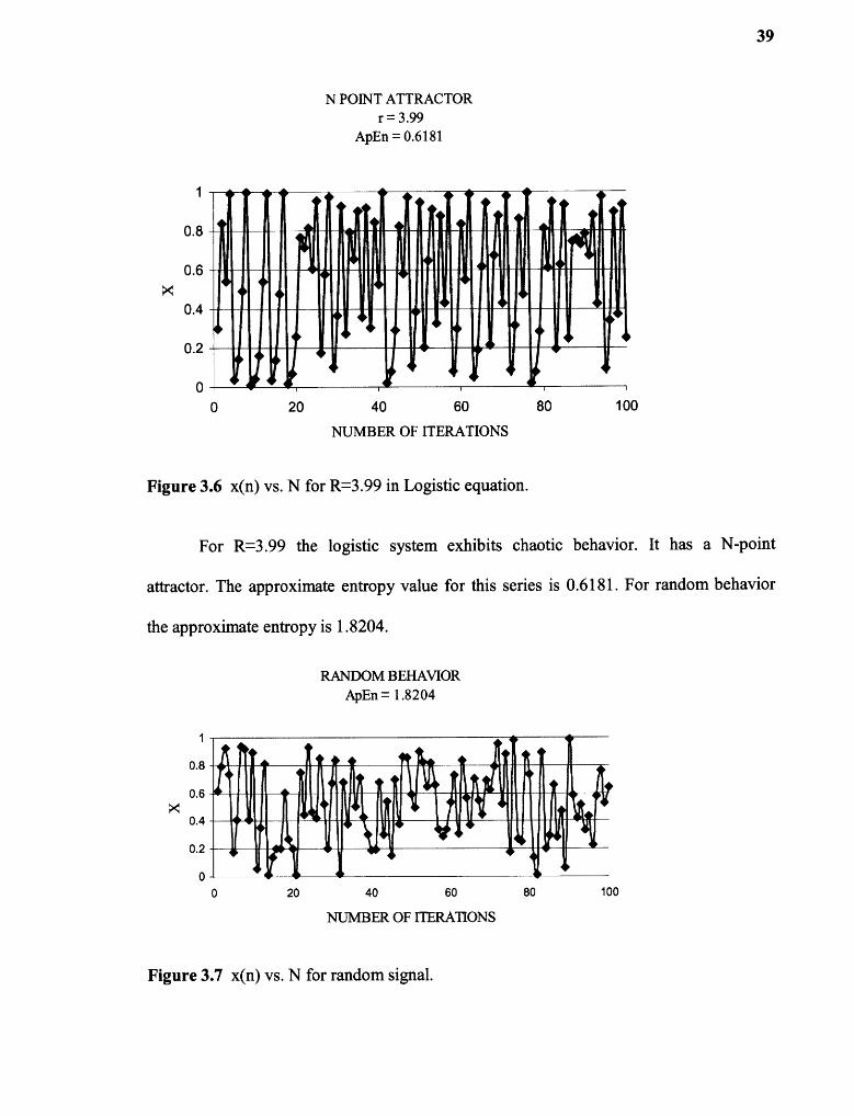
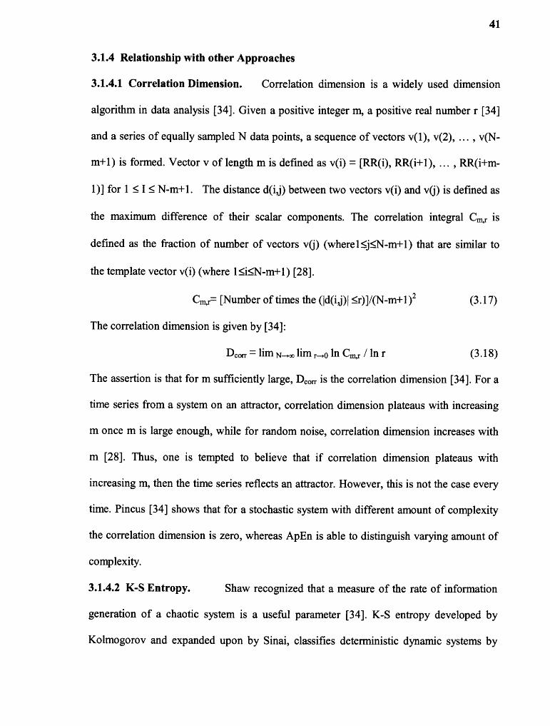
Figure 3.6 x(n) vs. N for R=3.99 in Logistic equation.
For R=3.99 the logistic system exhibits chaotic behavior. It has a N-point
attractor. The approximate entropy value for this series is 0.6181. For random behavior
the approximate entropy is 1.8204.
RANDOM BEHAVIORApEn = 1.8204
Figure 3.7 x(n) vs. N for random signal.

40
Thus, for the two opposite extremes: periodic and random behavior, the ApEn
values are very low and high respectively. Intermediate value corresponds to complex
behavior. However, one cannot certify chaos using ApEn. One can notice that numerical
values of ApEn correlate with the intuition of the complexity from the graphical
presentation of the time series.
A low value of ApEn might be because of two very different reasons: an increase
in the degree of regularity, or outlying data points. As discussed before, the regularity in
the time series causes the pattern vectors to repeat itself. This causes the conditional
probabilities to be nearly equal to 1, and results in low values of ApEn. However, the
presence of outliers or spikes in the time series causes the standard deviation to inflate.
This increases the similarity criterion `r', which results in more matches and in turn
produces a low value of ApEn. Therefore, the data set should be free of outliers.
A measure such as HR probably represents the output of multiple mechanisms,
including coupling interactions such as sympathetic/parasympathetic response and
external inputs from internal and external sources [35]. Greater non-linearity and
stochastic influence, visually manifested as a highly complex and random structure [35],
is seen in RR interval time series of humans. Pincus and Goldberger [35] hypothesize that
a wide class of disease and perturbations represent system decoupling and/or lessening of
external inputs, in effect isolating a central component from its ambient universe. ApEn
provides a means of assessing this hypothesis. Thus, a high value of ApEn of RR interval
time series usually corresponds to healthy conditions and a low value of ApEn usually
corresponds to pathology.
41
3.1.4 Relationship with other Approaches
3.1.4.1 Correlation Dimension. Correlation dimension is a widely used dimension
algorithm in data analysis [34]. Given a positive integer m, a positive real number r [34]
and a series of equally sampled N data points, a sequence of vectors v(1), v(2), , v(N-
m+1) is formed. Vector v of length m is defined as v(i) = [RR(i), RR(i+1), , RR(i+m-
1)] for 1 5 I 5_ N-m+1. The distance d(i,j) between two vectors v(i) and v(j) is defined as
the maximum difference of their scalar components. The correlation integral Cmr is
defined as the fraction of number of vectors v(j) (where15.1-m+1) that are similar to
the template vector v(i) (where 15_i5_N-m+1) [28].
Cm,r= [Number of times the (|d(i,j)|≤r)]/(N-m+1)2 (3.17)
The correlation dimension is given by [34]:
= lim N->∞ lim r->0 In Cm,r/In r (3.18)
The assertion is that for m sufficiently large, Dew is the correlation dimension [34]. For a
time series from a system on an attractor, correlation dimension plateaus with increasing
m once m is large enough, while for random noise, correlation dimension increases with
m [28]. Thus, one is tempted to believe that if correlation dimension plateaus with
increasing m, then the time series reflects an attractor. However, this is not the case every
time. Pincus [34] shows that for a stochastic system with different amount of complexity
the correlation dimension is zero, whereas ApEn is able to distinguish varying amount of
complexity.
3.1.4.2 K-S Entropy. Shaw recognized that a measure of the rate of information
generation of a chaotic system is a useful parameter [34]. K-S entropy developed by
Kolmogorov and expanded upon by Sinai, classifies deterministic dynamic systems by

42
rates of information generation [37]. The Eckmann - Ruelle formula to calculate rate of
information generation based on K-S entropy is given by [34]:
E-R entropy =lim r->0 limm->∞limN->∞[Φm,r-Φm+1,r] (3.19)
where (1)„1,r is defined in equation 3.3. E-R entropy is useful in classifying low
dimensional chaotic system; however, noise free and infinite amount of data is assumed
in its calculations [34]. It is usually infinite for stochastic process [37]. Since RR intervals
comprise both stochastic and deterministic components [37] and a large amount of noise
free data is hard to acquire, application of K-S entropy is difficult.
Heuristically, E-R entropy and ApEn measure the logarithmic likelihood that runs
of patterns that are close remain close on the next incremental comparisons [34]. A
nonzero value for the E-R entropy ensures that a known deterministic system is chaotic
[34]. E-R entropy is infinite for stochastic processes [34]. ApEn has three advantages in
comparison to K-S entropy [35]. ApEn is nearly unaffected by noise of magnitude below
the filter level r; is robust to occasional artifacts; and is finite for both stochastic and
deterministic process [35]. Thus, ApEn is closely related to K-S entropy because of
algorithm similarities but it is not an approximation of E-R entropy [34]. The building
block of the ApEn algorithm is the estimations of transition probabilities of the form:
{the probability that |v(j+m)-v(i+m)|≤s, given that |v(j+k)-v(i+k)|≤r for k=0,1,...,m-1}.
To calculate the K-S entropy, one would let m--÷00 and r-40. For N data points, these
transition probabilities cannot be well estimated for large m or small r, so a limiting
procedure cannot be undertaken without a massive amount of data [38]. Nonetheless,
there is substantial process information in these transition probabilities for fixed m and r,
which are used explicitly to form ApEn. The intuition motivating ApEn is that if joint
43
probability measures for reconstructed dynamics that describe each of two systems are
different, then their marginal distribution on a fixed partition are likely different [38].
Since one is interested in distinguishing two systems, rather than in attempting to certify
chaos, one typically needs orders of magnitude fewer points to accurately estimate these
marginals than to accurately reconstruct the "attractor" measure defining the process [38].
To test the ability of K-S entropy, Correlation dimension and ApEn to distinguish
stochastic processes from each other, Pincus [37] has developed a mixture of
deterministic and stochastic processes called the MIX(p) process. MIX is family of
processes that samples a sine wave for P=0 and consists of independent, identically
distributed uniform random variables from an interval for P=1, intuitively becoming more
random as P increases as illustrated in Fig 8a, 8b and 8c for P=0.1, 0.4 and 0.8
respectively [34]. To define the MIX process, let 0 5_ P 5_ 1. Let Xj = '\I2 sin(24/12) for
all j, Yj = i.i.d. uniform random variables on [43;0], and Zj=i.i.d. random variables, Zj
= 1 with probability P, Zj = 0 with probability 1-P. Then MIX (P)j = (1-Zj)Xj + ZjYj.
The MIX process has mean 0 and SD 1 for all P. [34].
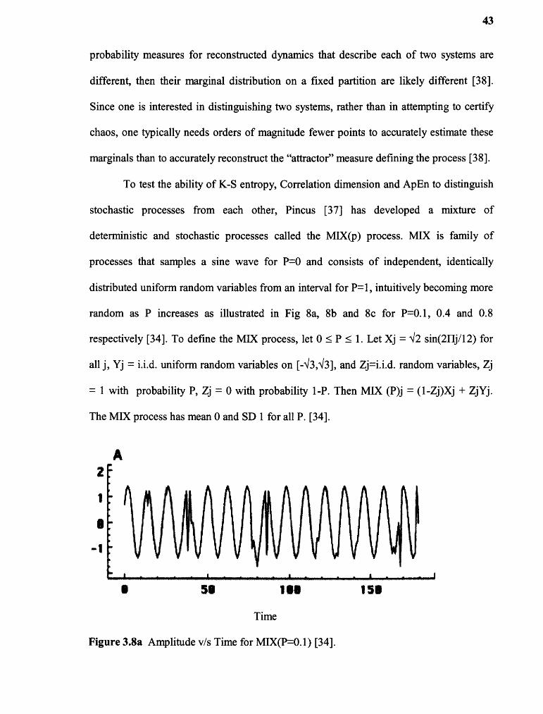
Figure 3.8a Amplitude v/s Time for MIX(P=0.1) [34].
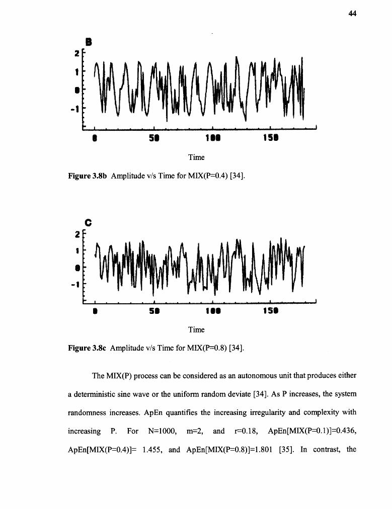
Figure 3.8b Amplitude v/s Time for MIX(P=0.4) [34].
44
Figure 3.8c Amplitude v/s Time for MIX(P=0.8) [34].
The MIX(P) process can be considered as an autonomous unit that produces either
a deterministic sine wave or the uniform random deviate [34]. As P increases, the system
randomness increases. ApEn quantifies the increasing irregularity and complexity with
increasing P. For N=1000, m=2, and r=0.18, ApEn[MIX(P=0.1)]=0.436,
ApEn[MIX(P=0.4)]= 1.455, and ApEn[MIX(P=0.8)]=1.801 [35]. In contrast, the

45
correlated dimension of MIX(P)=0 for all P<1, and the K-S entropy of MIX(P)=oc for all
P>0 [35]. Thus even given no noise and an infinite amount of data, these latter do not
discriminate the MIX(P) family [35].
Various complexity statistics like K-S entropy, Correlation dimension, etc.
developed to detect chaos from a time series work well with true dynamical systems as
these methods employ embedding dimension larger than m=2, as is typically employed
with ApEn [34]. In a purely deterministic dynamical system, they are more powerful than
ApEn in that they reconstruct the probability structure of the space with greater detail
[34]. However, they give confounding results for a system with both deterministic and
stochastic components and require large amount of noise free data [34].
3.1.5 Advantages and Disadvantages
The ApEn statistic may be calculated for a relatively short (1000 data points in case of
RR interval time series) series of noisy data [1]. It can give statistically accurate results
compared to the K-S entropy and Correlation dimension, whose values for certain
settings are undefined or infinity [34]. It can potentially distinguish a wide variety of
systems: low-dimensional deterministic systems, periodic and multiple periodic systems,
high-dimensional chaotic systems, stochastic and mixed systems [34]. The form of ApEn
provides for both de facto noise filtering, via choice of `r', and artifact insensitivity [37].
The numerical calculation of ApEn generally concurs with pictorial intuition, both for
theoretical and clinically derived data [37].
The order of the data is integral to the calculation of ApEn and must be preserved
during the data harvest [1]. Significant noise compromises meaningful interpretation of
ApEn [1]. ApEn is a biased statistic as 1) it depends on length of the time series and 2) it

46
counts self-matches. The statistic ApEn(m,r,N) is an estimate of the parameter
ApEn(m,r). Although the expected value of statistic ApEn increases asymptotically with
N to parameter ApEn, it is still a cause of bias [35]. Therefore, N must be same while
ApEn values of two time series are compared. The ApEn algorithm counts each sequence
as matching itself to avoid the occurrence of in (0) in calculations [37]. This leads to poor
self-consistency i.e., if ApEn of one data is higher than that of another, it should, but does
not, remain higher for all conditions tested [6]. If no patterns are repeated in the time
series than, intuitively, the ApEn should be high but because of self-matches it is equal to
zero. This is a strong source of bias. To elaborate this further, let us redefine the
conditional probability associated with the template vector v(i) of length m by letting Bi
denote the number of vector v(j) of length m with j # i, such that |d(i,j)|<=r by Ai [7].
Therefore, ApEn = - Σ i In [ WAN {1+Bi} ]/(N-m). For a time series in which patterns of
vectors are not repeated, intuitively, ApEn should be very high. But in such a random
time series, the templates are not repeated. Therefore, Bi and Ai are equal to zero. Hence
the conditional probability is equal to one and thus ApEn is equal to zero. This is
obviously inconsistent with the idea of new information and is a strong source of bias
toward conditional probability equal to 1 when there are few matches and A and B are
small [6]. The most straightforward way to e-inate the bias would be to remove self-
matching from the ApEn algorithm, leaving it otherwise unaltered [6]. However, without
the inclusion of self-matches, the ApEn algorithm is not defined unless Cm+i,r(i) > 0 for
every i. Removing self-matches would make ApEn statistics highly sensitive to outliers;
if there were a single template that matched no other vector, ApEn could not be
calculated because of the occurrence of ln(0) [6].

47
For a periodic system the value of ApEn will be very low; while, for a non-linear
and stochastic behavior the value of ApEn is high. ApEn cannot certify chaos unlike K-S
entropy [37] because ApEn has intermediate value for both non-linear deterministic and
stochastic process as seen in the case of MIX process, the Logistic equation and the
Henon equation.
3.2 Sample Entropy
An inherent bias within the ApEn calculation as discussed before has led to the
development of new family of statistics named sample entropy (SampEn) by Richman
and Moorman [6]. In sample entropy, self-matches are excluded from analysis to reduce
the bias. The name refers to the applicability to time series data sampled from a
continuous process [6].
3.2.1 Algorithm
In order to find the sample entropy of a given time series of N evenly sampled data
points, a subsequence of N-m vectors is formed, where `m' is the embedding dimension.
Each vector consists of m consecutive points. Each vector is compared with all other
vectors (excluding itself) in the time series to determine the probability that the distance
between two sequences of length m is within the tolerance `r'. Also the probability that
the distance between two sequences of length m+1 is within the tolerance 'r' is
determined. SampEn is the natural logarithm of the ratio of these probabilities.
A given RR interval time series of equally sampled N data points is divided into
subsequences of vectors `NT' of length `m', where v(i)=(RR[i], RR[i+1], RR[i+2],...,
RR[i+m-2],RR[i+m-l]) for 1 i N-m. Only first N-m vectors of length m are
48
considered to ensure that for 1 5. i N-m, both v. (i) and vm+1(i) defined. The distance
d(i,j) between two vectors vm(i) and vm(j) is defined as the maximum difference between
the scalar components of the two vectors. The two vectors are similar to each other if the
distance between the two vectors is less than r i.e., (|d(i,j)|<=r). The time series is
evaluated for pattern vectors that are repeated in the time series. The number of vectors
vm(j) (1 5. j N-m and j *i to exclude self-matches) similar to the template vector vm(i) is
given by:
Bi = number of vectors vm(j) such that |d(i,j)|<=r (3.19)
The probability of occurrence of vectors that are similar to the template vector is given
by:
Cm,r(i)= Bi /(N-m-1) (3.20)
The probability that two sequences match for m points is given by:
Bm,r = (Σi Cm,r(i))/(N-m) for 1 i 5_ N-m (3.21)
Similarly, the number of vectors vm+ 1(j) (1 j N-m and j A to exclude self-matches)
similar to the template vector vm+1 (i) is given by:
Ai = number of vectors vm+1(j) such thatld(i,j)|<=r (3.22)
The probability of occurrence of vectors that are similar to the template vector is given
by:
Cin+i,r(i)= A i /(N-m-1) (3.23)
The probability that two sequences match for m+1 points is given by:
Am,r = (Σi Cm+i,r(i))/(N-m) for 1 5. i 5. N-m (3.24)
The parameter SampEn is defined as [6]:
SampEn(m,r) = limN->∞ [-ln (Am,r /Bm,r )] (3.25)

49
The parameter SampEn(m,r) is estimated by statistic SampEn(m,r,N) [6] as:
SampEn(m,r,N) = [-In (Am,r /Bm,r )] (3.26)
Let B={[(N-m-1)(N-m)]/2}B nv and A = {RN-m-1)(N-m]/2} Am,r so that B is the total
number of template matches of length m and A is the total number of forward matches of
length m+1 [6]. Now A/B= (Am,r/Bm,r ), so statistic SampEn is given by:
SampEn(m,r,N) = -ln (A B) (3.27)
The quantity AB is precisely the conditional probability that two sequences within a
tolerance r for m points remain within r of each other at the next point [6]. The largest
possible value of SampEn statistic is ln(N-m)+ln(N-m+1)-ln(2) [6]. Thus, SampEn
statistic has nearly double the dynamic range than ApEn statistic [6]. There are two major
differences between SampEn and ApEn algorithms [6]. First, SampEn does not count
self-matches. Second, SampEn does not use a template wise approach when estimating
conditional probabilities [6]. Only one match is required for SampEn to be defined unlike
in ApEn where the match should be defined for each i. In contrast to ApEn(m,r,N), which
calculates probabilities in a template-wise fashion, SampEn(m,r,N) calculates the
negative algorithm of a probability associated with the series as a whole [6].
SampEn(m,r,N) will be defined except when B=0, in which case no regularity has been
detected, or when A=0, which corresponds to a conditional probability of 0 and an
infinite value of SampEn(m,r,N) [6].
3.2.2 Implementation
To implement the sample entropy algorithm, one has to define the length 'm' of the
pattern vector, the tolerance factor 'r' and the length 'N' of the time series. Based on
calculations that included both theoretical analysis and clinical applications, Richman and
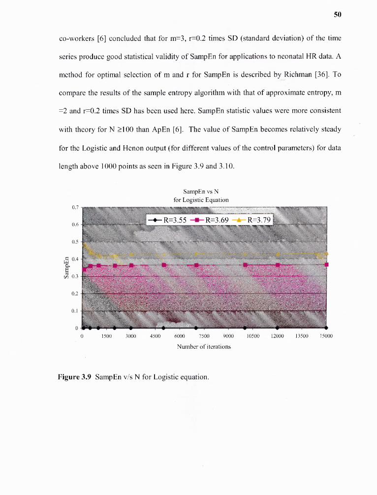
50
co-workers [6] concluded that for m=3, r=0.2 times SD (standard deviation) of the time
series produce good statistical validity of SampEn for applications to neonatal HR data. A
method for optimal selection of m and r for SampEn is described by Richman [36]. To
compare the results of the sample entropy algorithm with that of approximate entropy, m
=2 and r=0.2 times SD has been used here. SampEn statistic values were more consistent
with theory for N ...100 than ApEn [6]. The value of SampEn becomes relatively steady
for the Logistic and Henon output (for different values of the control parameters) for data
length above 1000 points as seen in Figure 3.9 and 3.10.
Figure 3.9 SampEn v/s N for Logistic equation.

Figure 3.10 ApEn v/s N for Henon equation.
Similar to the ApEn statistic, the SampEn statistic cannot distinguish between the
Logistic output and the Henon output as the value of SampEn is not much different.
However, similar to the ApEn statistic, it is able to distinguish the behavior of the system
on the basis of complexity of the output, as seen from the Table 3.2.
Table 3.2 Sampen (2,R,N) Calculations for Two Deterministic Models
Model Control Mean Std, r SampEn (2,r,N) r SampEn (2,r,N) r SampEn (2,r,N)
Type Param, Dev, N=500 N=1000 N=5000 N=500 N=1000 N=5000 N=500 N=1000 N=5000
Logistic 3,55 0.6477 0,2139 0.2 0 0 0 0,05 0 0 0 0.5 0,0081 0.004 0.0008
Logistic 3,69 0,6686 0,2009 0,2 0,3604 0,3633 0,3665 0.05 0,3614 0,3775 0.3833 0,5 0.3197 0.3242 0,3282
Logistic 3.79 0.646 0,2413 0,2 0,4401 0,4248 0.4304 0,05 0,4253 0.4263 0,4391 0,5 0,4232 0.4125 0,4126
a=-
Henon 1,b=0,48 0.2857 0,8774 0.2 0,2373 0,2343 0,2413 0,05 0,2493 0.2292 0,2503 0,5 0.1516 0,1558 0,1618
a=-
Henon 1.4,b=0.3 0,2624 0,7171 0.2 0,4801 0.4711 0.4652 0.05 0,5349 0,5204 0,5195 0,5 0.4502 0.4426 0,4393
51

52
3.2.3 Interpretation
The interpretation of sample entropy is similar to that of approximate entropy as
explained earlier. For a periodic system the value of SampEn will be very low, while for
a non-linear deterministic and stochastic behavior the value of SampEn is high.
Pincus and Goldberger [35] hypothesize that a wide class of disease and
perturbations represent system decoupling and/or lessening of external inputs, in effect
isolating a central component from its ambient universe. SampEn provides a means of
assessing this hypothesis. A high value of SampEn of RR interval time series corresponds
to healthy conditions and a low value corresponds to pathology.
3.2.4 Comparison with ApEn
For most processes, both ApEn and SampEn are expected to have two properties. First,
ApEn(m,r,N) and SampEn(m,r,N) should increase as r decreases [6]. Intuitively, as the
similarity criterion r becomes smaller, the conditional probability that sequences within r
of each other remain within r reduces, indicating that the series is less periodic and thus
resulting in larger values of both ApEn and SampEn. Second, ApEn and SampEn should
be independent of the length of the time series [6]. ApEn and SampEn statistic are tested
on uniform, independent, identically distributed random numbers. Uniform, independent,
identically distributed random numbers are used for testing because the conditional
probability can be calculated analytically based on their probabilistic distribution and
further, the theoretical values of ApEn and SampEn are nearly identical [6].

53
Figures 3.11 and 3.12 shows the performance of ApEn(2,r,N) and SampEn(2,r,N)
on uniform, independent, identically distributed random variables. The theoretical values
calculated by Richman and co-workers [6] are also shown. The uniform, independent,
identically distributed random numbers were generated using inbuilt functions of
MATLAB 7.0. The ApEn and SampEn values for different r and N were obtained using
the MATLAB codes described in Appendix B. SampEn(2,r,N) very closely matches the
expected results for r 0.03 (Figure3.12) and N ?_ 100 (Figure 3.11), whereas
ApEn(2,r,N) differs markedly from expectations for N < 1000 (Figure 3.11) and r < 0.2
(Figure 3.12). The value of ApEn is very low for small r and is not consistent with our
intuition. This inconsistency is a result of self- matching in the ApEn algorithm discussed
earlier.
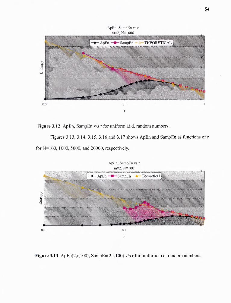
54
Figure 3.12 ApEn, SampEn v/s r for uniform i.i.d. random numbers.
Figures 3.13, 3.14, 3.15, 3.16 and 3.17 shows ApEn and SampEn as functions of r
for N=100, 1000, 5000, and 20000, respectively.
Figure 3.13 ApEn(2,r,100), SampEn(2,r,100) v/s r for uniform i.i.d. random numbers.
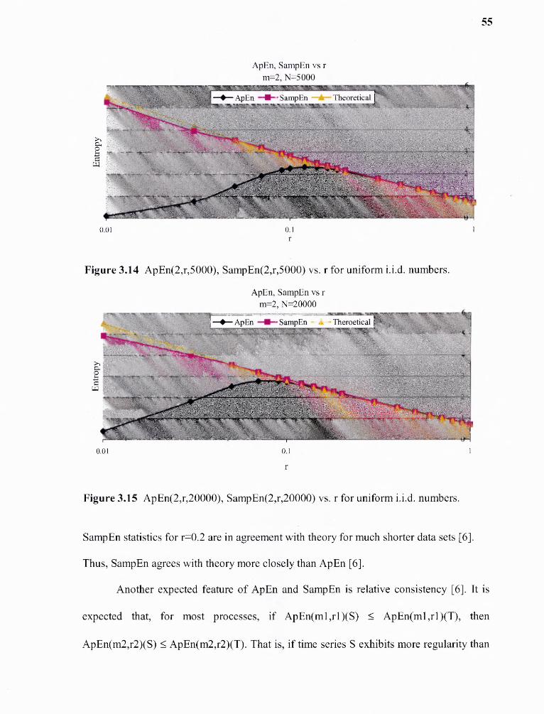
55
Figure 3.14 ApEn(2,r,5000), SampEn(2,r,5000) vs. r for uniform i.i.d. numbers.
Figure 3.15 ApEn(2,r,20000), SampEn(2,r,20000) vs. r for uniform i.i.d. numbers.
SampEn statistics for r=0.2 are in agreement with theory for much shorter data sets [6].
Thus, SampEn agrees with theory more closely than ApEn [6].
Another expected feature of ApEn and SampEn is relative consistency [6]. It is
expected that, for most processes, if ApEn(ml,rl)(S) ApEn(ml,rl)(T), then
ApEn(m2,r2)(S) ApEn(m2,r2)(T). That is, if time series S exhibits more regularity than

56
time series T for one pair of parameters m and r, it is expected to do so for all other pairs
[6]. Graphically, plots of ApEn and SampEn as a function of r for different data sets
should not cross over one another. The determination that one set of data exhibits greater
regularity than another can be made only when this condition is met. Richman and co-
workers [6] tested this expectation using 1000-point realizations of the MIX(p) process.
They found that relative consistency is maintained by SampEn but not by ApEn for
MIX(0.1) and MIX(0.9) processes. Thus, SampEn statistic shows relative consistency
where ApEn does not [6].
3.2.5 Advantages and Disadvantages
The advantages of the SampEn statistic are similar to those of the ApEn statistic. The
SampEn statistic can be calculated for shorter series of noisy data. Similar to the ApEn
statistic, the SampEn statistic is able to distinguish a wide variety of systems: low-
dimensional deterministic systems, periodic and multiply periodic systems, high-
dimensional chaotic systems, stochastic and mixed systems. The numerical calculation of
SampEn generally concurs with pictorial intuition, both for theoretical and clinically
derived data. In addition to that, the SampEn statistic agrees much better than the ApEn
statistic with theory for random numbers with known probabilistic character over a broad
range of operating conditions [6]. The SampEn statistic maintains relative consistency
where ApEn statistics do not [6].
The order of the data, just like with ApEn, is integral to the calculation of
SampEn and must be preserved during the data harvest. As discussed earlier, the SampEn
statistic maintains relative consistency where ApEn statistics do not [6]. However, there
is no general reason why ApEn or SampEn statistics should remain relatively consistent

57
for all time series and all choices of parameters [6]. SampEn is an event counting
statistic, where events are instances of vectors being similar to one another [6]. When
these events are sparse, the statistics are expected to be unstable, which might lead to lack
of relative inconsistency [6]. Suppose SampEn(m,r,N)(S) SampEn(m,r,N)(T) and that
the number of T's template matches, B t, is less than the number of S's template matches,
B„ which would be consistent with T displaying less order than S. Provided A t and As,
the number of forward matches, are relatively large, both SampEn statistics will be
considerably lower than their upper bounds [6]. As r decreases, B t and A t are expected to
decrease more rapidly than B s and A. Thus, as Bt becomes very small,
SampEn(m,r,N)(T) will begin to decrease approaching the value ln(Bt), and could cross
over a graph of SampEn(m,r,N)(S), where or while Bs is still relatively large.
Furthermore, as the number of template matches decreases, small changes in the number
of forward matches can have a large effect on the observed conditional probability [6].
Thus the discrete nature of the SampEn probability estimation could lead to small degrees
of cross over and intermittent failure of relatively consistency [6].
3.3 Multi-Scale Entropy
Classical entropy and physiologic complexity concepts do not have straightforward
correspondence [39]. Entropy is related to the degree of randomness of a time series and
it is maximum for completely random signals. Complexity is related to the underlying
structure of a time series and its information content [39]. An increase of the entropy
assigned to a time series usually, but not always, corresponds to an increase of underlying
system complexity. For instance, a randomized time series has higher entropy than the

58
original time series, although the process of generating the randomized data destroys
correlations and degrades the information content of the original signal [40].
Diseased systems, when associated with the emergence of more regular behavior
show reduced entropy values compared to the dynamics of free running healthy systems
[40]. However, certain pathologies, like atrial fibrillation, are associated with highly
erratic fluctuations with statistical properties resembling uncorrelated noise [40]. ApEn
and SampEn statistics will yield an increase in entropy for such physiologic signal when
compared to healthy dynamics showing correlated 1/f-type properties, even though the
latter represent a more physiologically complex state. This inconsistency may be related
to the fact that these statistics are based on single scale analysis and do not take into
account the complex temporal fluctuations inherent in healthy physiologic control system
[40]. Multi-scale entropy analysis is a new method of measuring the complexity, at
different time scales, of finite length time series. It was developed by Goldberger and co-
workers [41].
3.3.1 Algorithm
The MSE method consists of two procedures:
1. A "coarse-graining" process is applied to the time series. For a given RR interval
time series, {xi, x2,..., xN}, multiple coarse-grained series are constructed by averaging
the data points within non-overlapping windows of increasing length s [41]. Each
element of the coarse-grained time series, y(j), is calculated according to the equation:
y(j)s = (1/s) Σ i x(i) (3.28)
where ((j-1)s +1) i js, s represents the scale factor and j N/s. The length of each
coarse-grained time series is N/s. The scale factor specifies the number of data points

59
averaged to obtain each element of the coarse-grained time series. Figure 3.16 shows this
process for scale 2 and 3.
Figure 3.16 Schematic illustration of the coarse-graining procedure for scale 2 and 3[40].
For scale 1 the coarse-grained time series is simply the original time series.
2. SampEn is calculated for each coarse-grained time series, and then plotted as a
function of the scale factor [41]. SampEn is described earlier.
3.3.2 Implementation
To implement the multi-scale entropy algorithm, one has to define the length 'N' of the
time series, maximum scale factor s and parameters m and r for calculating the sample-
entropy of the coarse-grained time series. The multi-scale entropy is found for scale
factors from 1 to 20. To have sufficient data points in the coarse-grained time series at the
maximum scale factor, the length of the data is chosen to be 40000 points. This ensures
that at scale factor of 20, the length of the coarse-grained time series is 2000, sufficient to
find the sample entropy of the time series. As discussed earlier, m = 2 and r = 0.15 X SD.
r=0.15 X SD for all groups corresponds to normalizing all time series by their SD [40].
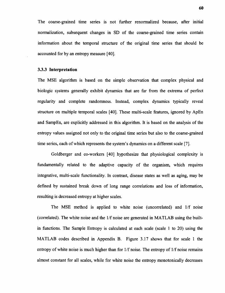
60
The coarse-grained time series is not further renormalized because, after initial
normalization, subsequent changes in SD of the coarse-grained time series contain
information about the temporal structure of the original time series that should be
accounted for by an entropy measure [40].
3.3.3 Interpretation
The MSE algorithm is based on the simple observation that complex physical and
biologic systems generally exhibit dynamics that are far from the extrema of perfect
regularity and complete randomness. Instead, complex dynamics typically reveal
structure on multiple temporal scales [40]. These multi-scale features, ignored by ApEn
and SampEn, are explicitly addressed in this algorithm. It is based on the analysis of the
entropy values assigned not only to the original time series but also to the coarse-grained
time series, each of which represents the system's dynamics on a different scale [7].
Goldberger and co-workers [40] hypothesize that physiological complexity is
fundamentally related to the adaptive capacity of the organism, which requires
integrative, multi-scale functionality. In contrast, disease states as well as aging, may be
defined by sustained break down of long range correlations and loss of information,
resulting is decreased entropy at higher scales.
The MSE method is applied to white noise (uncorrelated) and 1/f noise
(correlated). The white noise and the 1/f noise are generated in MATLAB using the built-
in functions. The Sample Entropy is calculated at each scale (scale 1 to 20) using the
MATLAB codes described in Appendix B. Figure 3.17 shows that for scale 1 the
entropy of white noise is much higher than for 1/f noise. The entropy of 1/f noise remains
almost constant for all scales, while for white noise the entropy monotonically decreases
61
with scale such that for scales larger than 4 it is lower than the entropy of 1/f noise [40].
This result is consistent with the fact that, unlike white noise, 1/f noise contains structures
across multiple time scales [39]. The white noise generates more information at scale
one, but the rate of information generation decreases at higher time scales; whereas, for
1/f noise, the rate of information generation is not high as compared to the white noise at
scale one, but the rate of information generation is higher at higher scales. This shows
that the 1/f behavior appears to be more complex than the white noise, when observed at
different scales.
Figure 3.17 MSE analysis of white noise and 1/f noise.
CHAPTER 4
DATA ACQUISTION AND ANALYSIS
4.1 Data Acquisition
As discussed earlier in section 1.2, the aim of this thesis is 1) to find how these entropy
measures differ in healthy and diseased subjects and 2) to find the effect of activity on
these measures. The RR interval time series data for task 1 is available on the website
www.physionet.org . The data for the normal control group were obtained from 24-hour
Holier monitor recordings of 44 subjects (men and women aged 20-76 years) from the
PhysioNet normal sinus rhythm database with ECG data sampled at 128 Hz. The data for
the congestive heart failure (CHF) group were obtained from 24 Holter recordings of 18
subjects (men and women aged 22-79 years) with ECG recordings sampled at 250 Hz.
The time at which these data were acquired, however, is not known. The data for task 2
were obtained from apparently normal subjects (3 men aged 22-27 years) using a Polar
S810 Heart Rate Monitor (accuracy of heart rate measurement is —1 to +1 beats per
minute). The monitor records the RR interval. The data were recorded when the subjects
were doing various activities. The protocol was as follows:
Standing: The subjects were allowed to stand at a particular place for 20 minutes
and were allowed to do nothing. The last thousand RR intervals were used for the
calculation of entropy measures.
Sitting on a chair: the subjects were allowed to sit on a chair and to read a book.
Data acquisition time was 20 minutes. The last thousand RR intervals were used for the
calculation of entropy measures.
62

63
Exercise: The subjects were asked to ride an exercise bike with an ergometer
(which can measure the amount of calories burned by the rider). The subjects were
allowed to warm up for 1 minute. The subject performed exercise for 15 minutes. Various
parameters like age, weight, number of calories to burn, etc., were kept same so that the
subjects were subjected to the same amount of load. They were allowed to ride the bike at
100 rpm. The last thousand RR intervals were used for the calculation of entropy
measures.
Paced Breathing: The subjects controlled their breathing for 15 minutes. The
breathing was paced using a device that flashed LEDs in a sequence. The LED are
arranged in a vertical position. Flashing sequence is such that first the LEDs flash from
bottom to top and then from top to bottom. The whole sequence is repeated 12 times in a
minute. Thus, if one synchronizes their breathing with the flashing sequence, the
breathing is paced at 12 breathes per minute. The last thousand RR intervals were used
for the calculation of entropy measures.
Two sets of readings were obtained for each subject on two different days
between 4 and 8 P.M. The recordings took place at the athletic center of NJIT and the
Biomedical Signal Processing Lab at NJIT.
4.2 Data Anomalies and Correction
The data, discussed in the previous section, contained sporadic entries that were too high
or too low to be considered as a part of the data set. These sporadic entries are called
outliers. Outliers have detrimental effects on the calculation of the entropy measures
because outliers increase the standard deviation of the time series. This unnecessarily

64
increases the tolerance factor 'r' and subsequently reduces the entropy. Such entries were
removed from the data set using a "deglitching" code [Appendix B] available on
PhysioNet. The code is written in MATLAB. The code identifies the outliers by
comparing the data set with an Auto Regressive prediction model of order 3. If the data
point is within 25% to 75% of the predicted value, than the point is labeled valid,
otherwise invalid. Only valid points are used to calculate the entropy measures.
4.3 Programs for Data Analysis
The computer programs used to calculate ApEn, SampEn and MSE are written in
MATLAB. They are based on the algorithms explained in chapter 3. The codes
[Appendix B] for ApEn and SampEn are available on PhysioNet and are classified as
Class 1 software (extensively and rigorously tested software). The author of this thesis
wrote the MATLAB program for MSE analysis. The sample entropy calculation in the
MSE program is, however, done using the SampEn program from PhysioNet.
4.4 Results of Data Analysis
The results of various entropy measures obtained from the RR interval data of normal
sinus rhythm (NSR) and congestive heart failure (CHF) subjects are provided. The
sample entropy obtained from the RR interval data of apparently healthy subjects during
various activities (described earlier) is also displayed.
Table 4.1 shows the effect of length on the value of ApEn for NSR subjects. Table 4.2
shows the variation in value of ApEn during the recording for NSR subjects. Table 4.3
shows the effect of length on the value of ApEn for CHF subjects. Table 4.4 shows the

65
variation in value of ApEn during the recording for CHF subjects. As can be seen in these
tables, the ApEn values are higher for the NSR group than the CHF group. The ApEn
value for the NSR group is 0.99 ± 0.21 (mean ± standard deviation) while, 0.82 ± 0.23
(mean ± standard deviation) for the CHF group for the first thousand data points. Also,
27 subjects out of a total of 44 NSR subjects have ApEn(2,0.2,1000) > 0.9 as seen in
Table 4.1. Also, 12 subjects out of a total of 18 CHF subjects have ApEn(2,0.2,1000) <
0.9 as seen in Table 4.3. The true positive specificity is 0.61. The true negative specificity
is 0.67. The false positive specificity is 0.33. The false negative specificity is 0.39.

Table 4.1 Apen(2,0.2,N) vs. Data Lengths for NSR Subjects
DataLength 500 1000 2000 3000 4000 5000 10000 20000 30000 40000SubjectNSR001 0.9228 0.8866 0.8026 0.7333 0.7132 0.7222 0.7462 0.45 0.8744 0.916NSR002 1.1564 1.1372 0.9718 0.9982 0.9804 0.9682 0.9413 1.017 1.0941 1.1282NSR003 1.2096 0.9913 0.9251 0.8642 0.9083 0.9421 0.9163 0.8567 0.7757 0.7627NSR004 0.919 0.6686 0.5831 0.6136 0.6774 0.6056 0.6805 0.8559 0.8141 0.74NSR005 0.8329 0.8959 0.9423 0.7526 0.9027 0.7167 0.7421 0.7052 0.7115 0.5272NSR006 1.018 1.0067 0.8684 0.9032 0.6241 0.6192 0.6122 0.5324 0.6524 0.7457NSR007 1.0232 1.0747 0.8534 1.0372 1.0352 1.0166 0.4326 0.5709 0.5037 0.523NSR008 1.1526 1.1883 1.2403 1.2773 1.2939 1.2882 1.275 1.1959 1.1813 1.1796NSR009 1.2169 1.0074 0.9102 1.1007 1.0268 1.0032 0.9797 1.0795 0.9721 1.0503NSR010 0.9932 0.9481 0.9573 1.0649 1.0634 1.0704 0.9918 0.9631 0.9702 0.9872NSR011 1.2156 1.0136 1.0095 1.0098 1.0984 1.0218 0.976 1.1816 1.0157 1.0661NSR012 0.8083 0.6935 0.7666 0.8144 0.8248 0.8061 0.8995 0.9927 0.8337 0.6567NSR013 1.1308 1.2611 0.4418 0.3637 0.3641 0.3725 0.4844 0.6917 0.4301 0.4229NSR014 1.1219 1.159 1.2412 1.1642 0.7459 0.706 1.0317 0.9937 0.944 0.9737NSR015 1.1276 1.1124 1.1476 1.1915 1.2071 1.2401 1.2776 1.2621 1.3032 1.3225NSR016 1.0658 1.1056 1.2205 1.1898 1.2028 0.9418 1.1008 1.1026 1.0682 1.0799NSR017 0.7178 0.6677 0.6391 0.6581 0.6782 0.6729 0.7084 0.7716 0.797 0.4854NSR018 1.1709 1.2741 1.1562 1.1673 1.0568 0.964 1.0825 1.1797 1.1895 0.9201NSR019 0.9539 1.1438 1.1941 1.2337 1.1042 1.1488 1.1055 1.052 1.0739 0.7275NSR020 0.9975 1.2057 0.7052 0.6968 0.7149 0.7363 0.67 0.6939 0.7018 0.6916NSR021 0,7769 0.8797 0.3595 0.2987 0.2863 0.2719 0,2783 0.3693 0.3472 0.3897NSR022 1.1916 0.6364 0.6932 0.702 0.7397 0.7666 0.8405 0.9341 0.8578 0.5051NSR023 0.6685 0.7661 0.3488 0.3927 0.7186 0.7515 0.9306 0.619 0.6075 0.6318NSR024 0.8118 0.8585 0.8507 0.8356 0.8082 0.784 0.4899 0.4486 0.4916 0.5284NSR025 0.8748 0.8815 0.9312 0.9465 1.0109 0.9873 0.9784 0.8985 0.8331 0.9368NSR026 1.0362 0.9156 0.6067 0.6283 0.6608 0.8433 0.8879 0.8246 0.9004 0.7459NSR027 0.9199 0.75 0.5125 0.688 0.7646 0.7637 0.6596 0.5673 0.797 0.8254NSR028 0.8744 0.8077 0.8263 0.8707 0.8973 0.863 0.8405 0.7757 0.7195 1.5139NSR029 1.1312 1.2781 1.4978 0.9324 1.003 0.8739 0.7352 0.6934 0.7521 0.7408NSR030 1.1104 0.8792 0.8259 0.807 0.7949 0.8222 0.8669 0.8707 0.7411 0.5336NSR031 1.1502 0.7753 0.4145 0.3838 0.4036 0.4173 0.4434 0.7025 0.8535 0.7097NSR032 1.0834 1.2373 1.3315 1.3888 1.4009 0.925 1.1417 0.7187 0.7689 1.1261NSR033 0.8335 0.9224 0.9322 0.869 0.9527 0.963 0.9271 0.6756 0.6625 0.7034NSR034 1.1061 0.6835 0.7122 0.7085 0.7041 0.5722 0.8122 0.83 0.8398 0.6806NSR035 1.0598 0.7456 0.8024 0.8538 0.8652 0.8776 0.993 0.8299 0.8506 0.672NSR036 1.1936 1.3149 1.3356 1.3491 1.3364 1.3459 1.3705 1.4115 0.972 1.0174NSR037 1.1182 1.0419 1.0519 1.0937 1.0602 1.116 1.0088 0.7917 0.8623 0.8971NSR038 1.1025 1.1595 1.1974 1.2343 1.2566 1.2691 1.2458 1.2057 1.2282 1.2562NSR039 1.1976 0.931 1.0934 1.0606 1.0779 1.0738 1.0085 0.9238 0.9047 0.8941NSR040 1.1239 1.3272 0.8681 0.9368 0.9475 0.936 0.8925 0.8282 0.6592 0.8764NSR041 1.1564 1.3744 1.1609 1.2775 1.3234 1.2886 1.1864 0.8555 0.8182 0.8918NSR042 1.1349 0.7792 0.6919 0.647 0.7215 0.6196 0.8429 0.8258 0.9852 0.5381NSR043 1.1741 1.0626 1.0607 1.3369 1.5242 1.5395 1.3471 1.2791 1.0037 1.0285NSR044 1.0803 1.3081 0.9062 0.8901 0.9405 0.9387 1.0026 1.0481 1.0847 1.1711MEAN 1.0378 0.9945 0.8997 0.9083 0.9187 0.8903 0.8951 0.8654 0.8511 0.8346
66
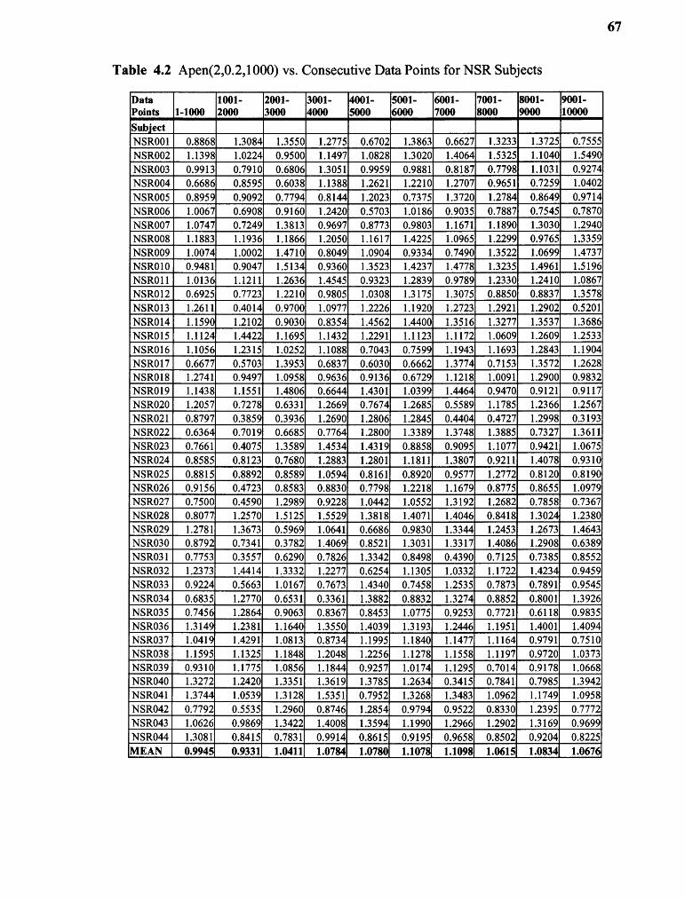
Table 4.2 Apen(2,0.2,1000) vs. Consecutive Data Points for NSR Subjects
DataPoints 1-1000
1001-2000
2001-3000
3001-4000
4001-5000
5001-6000
6001-7000
7001-8000
8001-9000
9001-10000
SubjectNSR001 0.8868 1.3084 1.3550 1.2775 0.6702 1.3863 0.6627 1.3233 1.3725 0.7555NSR002 1.1398 1.0224 0.9500 1.1497 1.0828 1.3020 1.4064 1.5325 1.1040 1.5490NSR003 0.9913 0.7910 0.6806 1.3051 0.9959 0.9881 0.8187 0.7798 1.1031 0.9274NSR004 0.6686 0.8595 0.6038 1.1388 1.2621 1.2210 1.2707 0.9651 0.7259 1.0402NSR005 0.8959 0.9092 0.7794 0.8144 1.2023 0.7375 1.3720 1.2784 0.8649 0.9714NSR006 1.0067 0.6908 0.9160 1.2420 0.5703 1.0186 0.9035 0.7887 0.7545 0.7870NSR007 1.0747 0.7249 1.3813 0.9697 0.8773 0.9803 1.1671 1.1890 1.3030 1.2940NSR008 1.1883 1.1936 1.1866 1.2050 1.1617 1.4225 1.0965 1.2299 0.9765 1.3359NSR009 1.0074 1.0002 1.4710 0.8049 1.0904 0.9334 0.7490 1.3522 1.0699 1.4737NSR010 0.9481 0.9047 1.5134 0.9360 1.3523 1.4237 1.4778 1.3235 1.4961 1.5196NSR011 1.0136 1.1211 1.2636 1.4545 0.9323 1.2839 0.9789 1.2330 1.2410 1.0867NSR012 0.6925 0.7723 1.2210 0.9805 1.0308 1.3175 1.3075 0.8850 0.8837 1.3578NSR013 1.2611 0.4014 0.9700 1.0977 1.2226 1.1920 1.2723 1.2921 1.2902 0.5201NSR014 1.1590 1.2102 0.9030 0.8354 1.4562 1.4400 1.3516 1.3277 1.3537 1.3686NSR015 1.1124 1.4422 1.1695 1.1432 1.2291 1.1123 1.1172 1.0609 1.2609 1.2533NSR016 1.1056 1.2315 1.0252 1.1088 0.7043 0.7599 1.1943 1.1693 1.2843 1.1904,NSR017 0.6677 0.5703 1.3953 0.6837 0.6030 0.6662 1.3774 0.7153 1.3572 1.2628NSR018 1.2741 0.9497 1.0958 0.9636 0.9136 0.6729 1.1218 1.0091 1.2900 0.9832NSR019 1.1438 1.1551 1.4806 0.6644 1.4301 1.0394 1.4464 0.9470 0.9121 0.9117NSR020 1.2057 0.7278 0.6331 1.2669 0.7674 1.2685 0.5589 1.1785 1.2366 1.2567NSR021 0.8797 0.3859 0.3936 1.2690 1.2806 1.2845 0.4404 0.4727 1.2998 0.3193NSR022 0.6364 0.7019 0.6685 0.7764 1.2800 1.3389 1.3748 1.3885 0.7327 1.3611NSR023 0.7661 0.4075 1.3589 1.4534 1.4319 0.8858 0.9095 1.1077 0.9421 1.0675NSR024 0.8585 0.8123 0.7680 1.2883 1.2801 1.1811 1.3807 0.9211 1.4078 0.9310NSR025 0.8815 0.8892 0.8589 1.0594 0.8161 0.8920 0.9577 1.2772 0.8120 0.8190NSR026 0.9156 0.4723 0.8583 0.8830 0.7798 1.2218 1.1679 0.8775 0.8655 1.0979NSR027 0.7500 0.4590 1.2989 0.9228 1.0442 1.0552 1.3192 1.2682 0.7858 0.7367NSR028 0.8077 1.2570 1.5125 1.5529 1.3818 1.4071 1.4046 0.8418 1.3024 1.2380NSR029 1.2781 1.3673 0.5969 1.0641 0.6686 0.9830 1.3344 1.2453 1.2673 1.4643NSR030 0.8792 0.7341 0.3782 1.4069 0.8521 1.3031 1.3317 1.4086 1.2908 0.6389NSR031 0.7753 0.3557 0.6290 0.7826 1.3342 0.8498 0.4390 0.7125 0.7385 0.8552NSR032 1.2373 1.4414 1.3332 1.2277 0.6254 1.1305 1.0332 1.1722 1.4234 0.9459NSR033 0.9224 0.5663 1.0167 0.7673 1.4340 0.7458 1.2535 0.7873 0.7891 0.9545NSR034 0.6835 1.2770 0.6531 0.3361 1.3882 0.8832 1.3274 0.8852 0.8001 1.3926NSR035 0.7456 1.2864 0.9063 0.8367 0.8453 1.0775 0.9253 0.7721 0.6118 0.9835NSR036 1.3149 1.2381 1.1640 1.3550 1.4039 1.3193 1.2446 1.1951 1.4001 1.4094NSR037 1.0419 1.4291 1.0813 0.8734 1.1995 1.1840 1.1477 1.1164 0.9791 0.7510NSR038 1.1595 1.1325 1.1848 1.2048 1.2256 1.1278 1.1558 1.1197 0.9720 1.0373NSR039 0.9310 1.1775 1.0856 1.1844 0.9257 1.0174 1.1295 0.7014 0.9178 1.0668NSR040 1.3272 1.2420 1.3351 1.3619 1.3785 1.2634 0.3415 0.7841 0.7985 1.3942NSR041 1.3744 1.0539 1.3128 1.5351 0.7952 1.3268 1.3483 1.0962 1.1749 1.0958NSR042 0.7792 0.5535 1.2960 0.8746 1.2854 0.9794 0.9522 0.8330 1.2395 0.7772NSR043 1.0626 0.9869 1.3422 1.4008 1.3594 1.1990 1.2966 1.2902 1.3169 0.9699NSR044 1.3081 0.8415 0.7831 0.9914 0.8615 0.9195 0.9658 0.8502 0.9204 0.8225MEAN 0.9945 0.9331 1.0411 1.0784 1.0780 1.1078 1.1098 1.0615 1.0834 1.0676
67
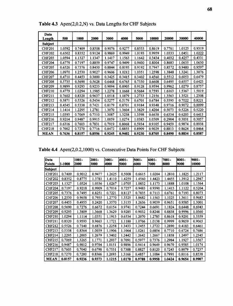
Table 4.3 Apen(2,0.2,N) vs. Data Lengths for CHF Subjects
DataLength 500 1000 2000 3000 4000 5000 10000 20000 30000 40000
SubjectCHF201 1.0592 0.7409 0.8508 0.9076 0.9277 0.8553 0.8619 0.7761 1.0125 0.9319CHF202 0.6502 0.8352 0.9124 0.9869 0.9949 1.0193 0.9959 1.0333 1.0451 1.0222CHF203 1.0594 1.1327 1.1347 1.1417 1.1563 1.1642 0.3434 0.4032 0.4257 0.4331CHF204 0.6779 0.7197 0.8859 0.9747 0.9499 0.9400 0.8004 0.8683 1.0635 1.0630CHF205 0.6526 0.7376 0.8450 0.8844 0.8193 0.9192 0.7947 0.8572 0.9480 0.9597CHF206 1.0970 1.2530 0.9027 0.9606 1.0212 1.0351 1.2598 1.3848 1.3241 1.3076CHF207 0.4710 0.4453 0.3800 0.3425 0.3415 0.3402 0.4560 0.5512 0.6053 0.6479CHF208 0.5735 0.5690 0.5628 0.6468 0.6765 0.7330 0.6608 0.6495 0.6557 0.6423CHF209 0.9899 0.9293 0.9233 0.9094 0.8905 0.9128 0.9594 0.9962 1.0279 0.8757CHF210 0.4779 1.0294 1.1985 1.2278 1.1668 0.5684 0.7593 1.6163 1.5367 1.5019CHF211 0.7602 0.8320 0.9637 1.0518 1.1879 1.2733 1.2156 1.3563 1.3521 1.2308CHF212 0.3871 0.5526 0.5434 0.5277 0.5179 0.6701 0.6784 0.5595 0.7022 0.8221CHF213 0.4545 0.5338 0.7421 0.8179 0.8701 0.9184 0.9348 0.9716 0.9072 0.8099CHF214 1.1414 1.2295 1.2781 1.3070 1.3604 1.3829 1.4204 0.5073 0.5226 0.5220CHF215 1.0393 0.7069 0.7310 1.3087 1.3238 1.3598 0.6638 0.6334 0.6203 0.6413CHF216 0.9214 0.9487 0.9915 1.0059 1.0274 1.0383 1.0509 0.2904 0.3031 0.3057CHF217 0.6316 0.7603 0.7831 0.7919 0.8068 0.5934 0.9105 0.9459 0.9874 0.8938CHF218 0.7002 0.7270 0.7716 0.8472 0.8855 0.8909 0.9029 0.8813 0.8624 0.8464MEAN 0.7636 0.8157 0.8556 0.9245 0.9402 0.9230 0.8705 0.8490 0.8834 0.8587
Table 4.4 Apen(2,0.2,1000) vs. Consecutive Data Points For CHF Subjects
DataPoints 1-1000
1001-2000
2001-3000
3001-4000
4001-5000
5001-6000
6001-7000
7001-8000
8001-9000
9001-10000
SubjectCHF201 0.7409 0.9012 0.9477 1.2625 0.5008 0.6615 1.0204 1.2810 1.1825 1.2117CHF202 0.8352 0.8775 1.3781 1.4110 1.4259 1.4560 1.4423 1.4455 1.3912 1.2947CHF203 1.1327 1.0524 1.0336 1.0267 1.0705 1.0832 1.1173 1.1888 1.0108 1.1564CHF204 0.7197 0.9218 0.9909 0.7016 0.7257 0.9483 0.9390 1.1415 1.1122 0.5204CHF205 0.7376 0.7495 0.8251 0.7221 0.8127 0.7835 0.7113 0.6761 0.7193 0.8073CHF206 1.2530 0.9658 0.7955 1.2770 1.3325 1.0682 1.1563 1.1025 1.3611 0.9683CHF207 0.4453 0.4955 0.2420 1.3570 1.3155 1.2636 0.9039 0.9651 0.9585 1.3001CHF208 0.5690 0.7276 0.6672 0.6154 0.9741 0.7244 0.6691 1.1824 0.6448 0.6943CHF209 0.9293 1.3809 1.3668 1.3629 0.9285 0.9032 0.8248 0.8838 0.9996 1.0360CHF210 1.0294 1.1114 1.0351 1.1913 0.6534 1.2070 1.2785 0.8618 0.9201 1.3359CHF211 0.8320 0.9593 0.9663 1.1721 1.1180 1.0766 1.0138 0.9999 0.9659 0.9065CHF212 0.5526 0.7140 0.6876 1.2258 1.3433 1.2455 1.2722 1.2890 0.4183 0.6461CHF213 0.5338 0.8364 1.0039 1.1906 1.1064 1.0261 0.6854 0.7710 0.6724 0.7686CHF214 1.2295 1.2005 1.2679 1.3402 1.2442 1.2642 1.2667 1.1858 1.2497 1.2345CHF215 0.7069 1.3265 1.1771 1.2937 0.7091 0.5977 0.7376 1.2984 1.1927 1.3567CHF216 0.9487 0.9812 0.9704 1.0151 0.9896 0.9414 0.9649 0.9670 0.9585 1.0174CHF217 0.7603 0.7040 0.6798 0.7531 0.7388 0.8827 0.8120 0.7243 0.8079 0.7237CHF218 0.7270 0.7200 0.8366 1.2693 1.3166 0.4857 1.1084 0.7991 0.8116 0.8538MEAN 0.8157 0.9236 0.9373 1.1215 1.0170 0.9788 0.9958 1.0424 0.9654 0.9907
68
69
Table 4.5 shows the effect of length on the value of SampEn for NSR subjects.
Table 4.6 shows the variation in the value of SampEn during the recording for NSR
subjects. Table 4.7 shows the effect of length on the value of SampEn for CHF subjects.
Table 4.8 shows the variation in the value of SampEn during the recording for CHF
subjects. As can be seen in these tables, the SampEn values are higher for the NSR group
than the CHF group. The SampEn value for the NSR group is 0.93 ± 0.28 (mean ±
standard deviation) while, 0.67 ± 0.27 (mean ± standard deviation) for the CHF group.
Also, 27 subjects out of a total of 44 NSR subjects have SampEn(2,0.2,1000) > 0.8 as
seen in Table 4.5. Also, 12 subjects out of a total of 18 CHF subjects have
SampEn(2,0.2,1000) < 0.8 as seen in Table 4.7. The true positive specificity is 0.61. The
true negative specificity is 0.67. The false positive specificity is 0.33. The false negative
specificity is 0.39.
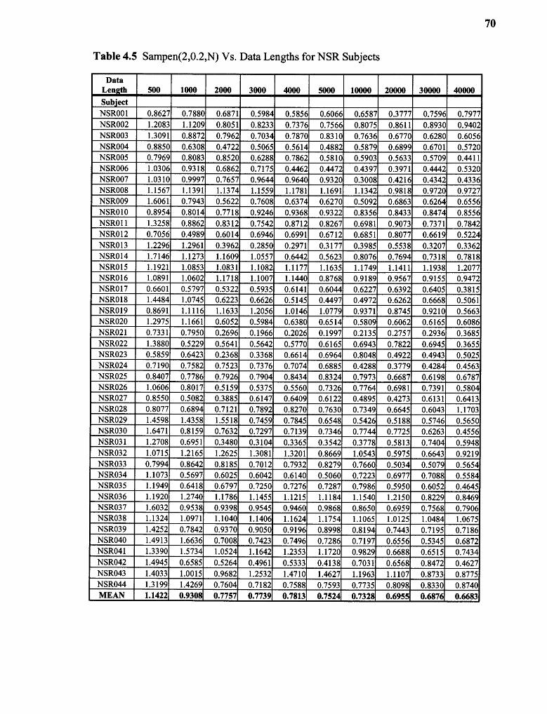
Table 4.5 Sampen(2,0.2,N) Vs. Data Lengths for NSR Subjects
DataLength 500 1000 2000 3000 4000 5000 10000 20000 30000 40000SubjectNSR001 0.8627 0.7880 0.6871 0.5984 0.5856 0.6066 0.6587 0.3777 0.7596 0.7977NSR002 1.2083 1.1209 0.8051 0.8233 0.7376 0.7566 0.8075 0.8611 0.8930 0.9402NSR003 1.3091 0.8872 0.7962 0.7870 0.8310 0.7636 0.6770 0.6280 0.6056NSR004 0.8850 0.6308 0.4722 0.5065 0.5614 0.4882 0.5879 0.6899 0.6701 0.5720NSR005 0.7969 0.8083 0.8520 0.6288 0.7862 0.5810 0.5903 0.5633 0.5709 0.4411NSR006 1.0306 0.9318 0.6862 0.7175 0.4462 0.4472 0.4397 0.3971 0.4442 0.5320NSR007 1.0310 0.9997 0.7657 0.9644 0.9640 0.9320 0.3008 0.4342 0.4336NSR008 1.1567 1.1391 1.1374 1.1559 1.1781 1.1691 1.1342 0.9818 0.9720 0.9727NSR009 1.6061 0.7943 0.5622 0.7608 0.6374 0.6270 0.5092 0.6863 0.6264 0.6556NSR010 0.8954 0.8014 0.7718 0.9246 0.9368 0.9322 0.8356 0.8433 0.8474 0.8556NSR011 1.3258 0.8862 0.8312 0.7542 0.8712 0.8267 0.6981 0.9073 0.7371 0.7842NSR012 0.7056 0.4989 0.6014 0.6946 0.6991 0.6712 0.6851 0.8077 0.6619 0.5224NSR013 1.2296 1.2961 0.3962 0.2850 0.2971 0.3177 0.3985 0.5538 0.3207 0.3362NSR014 1.7146 1.1273 1.1609 1.0557 0.6442 0.5623 0.8076 0.7694 0.7318 0.7818NSR015 1.1921 1.0853 1.0831 1.1082 1.1177 1.1635 1.1749 1.1411 1.1938 1.2077NSR016 1.0891 1.0602 1.1718 1.1007 1.1440 0.8768 0.9189 0.9567 0.9155 0.9472NSR017 0.6601 0.5797 0.5322 0.5935 0.6141 0.6044 0.6227 0.6392 0.6405 0.3815NSR018 1.4484 1.0745 0.6223 0.6626 0.5145 0.4497 0.4972 0.6262 0.6668 0.5061NSR019 0.8691 1.1116 1.1633 1.2056 1.0146 1.0779 0.9371 0.8745 0.9210 0.5663NSR020 1.2975 1.1661 0.6052 0.5984 0.6380 0.6514 0.5809 0.6062 0.6165 0.6086NSR021 0.7331 0.7950 0.2696 0.1966 0.2026 0.1997 0.2135 0.2757 0.2936 0.3685NSR022 1.3880 0.5229 0.5641 0.5642 0.5770 0.6165 0.6943 0.7822 0.6945 0.3655NSR023 0.5859 0.6423 0.2368 0.3368 0.6614` 0.6964 0.8048 0.4922 0.4943 0.5025NSR024 0.7190 0.7582 0.7523 0.7376 0.7074 0.6885 0.4288 0.3779 0.4284 0.4563NSR025 0.8407 0.7786 0.7926 0.7904 0.8434 0.8324 0.7973 0.6687 0.6198 0.6787NSR026 1.0606 0.8017 0.5159 0.5375 0.5560 0.7326 0.7764 0.6981 0.7391 0.5804NSR027 0.8550 0.5082 0.3885 0.6147 0.6409 0.6122 0.4895 0.4273 0.6131 0.6413NSR028 0.8077 0.6894 0.7121 0.7892 0.8270 0.7630 0.7349 0.6645 0.6043 1.1703NSR029 1.4598 1.4358 1.5518 0.7459 0.7845 0.6548 0.5426 0.5188 0.5746 0.5650NSR030 1.6471 0.8159 0.7632 0.7297 0.7139 0.7346 0.7744 0.7725 0.6263 0.4556NSR031 1.2708 0.6951 0.3480 0.3104 0.3365 0.3542 0.3778 0.5813 0.7404 0.5948NSR032 1.0715 1.2165 1.2625 1.3081 1.3201 0.8669 1.0543 0.5975 0.6643 0.9219NSR033 0.7994 0.8642 0.8185 0.7012 0.7932 0.8279 0.7660 0.5034 0.5079 0.5654NSR034 1.1073 0.5697 0.6025 0.6042 0.6140 0.5060 0.7223 0.6977 0.7088 0.5584NSR035 1.1949 0.6418 0.6797 0.7250 0.7276 0.7287 0.7986 0.5950 0.6052 0.4645NSR036 1.1920 1.2740 1.1786 1.1455 1.1215 1.1184 1.1540 1.2150 0.8229 0.8469NSR037 1.6032 0.9538 0.9398 0.9545 0.9460 0.9868 0.8650 0.6959 0.7568 0.7906NSR038 1.1324 1.0971 1.1040 1.1406 1.1624 1.1754 1.1065 1.0125 1.0484 1.0675NSR039 1.4252 0.7842 0.9370 0.9050 0.9196 0.8998 0.8194 0.7443 0.7195 0.7186NSR040 1.4913 1.6636 0.7008 0.7423 0.7496 0.7286 0.7197 0.6556 0.5345 0.6872NSR041 1.3390 1.5734 1.0524 1.1642 1.2353 1.1720 0.9829 0.6688 0.6515 0.7434NSR042 1.4945 0.6585 0.5264 0.4961 0.5333 0.4138 0.7031 0.6568 0.8472 0.4627NSR043 1.4033 1.0015 0.9682 1.2532 1.4710 1.4627 1.1963 1.1107 0.8733 0.8775NSR044 1.3199 1.4269 0.7604 0.7182 0.7588 0.7593 0.7735 0.8098 0.8330 0.8740MEAN 1.1422 0.9308 0.7757 0.7739 0.7813 0.7524 0.7328 0.6955 0.6876 0.6683
70

Table 4.6 Sampen(2,0.2,1000) vs. Consecutive Data Points for NSR Subjects
DataPoints 1-1000
1001-2000
2001-3000
3001-4000
4001-5000
5001-6000
6001-7000
7001-8000
8001-9000
9001-10000
SubjectNSR001 0.7880 1.5714 1.4555 1.4491 0.6150 1.5177 0.5865 1.6438 1.7371 0.6777NSR002 1.1209 0.9397 0.8402 1.0307 1.0766 1.2495 2.2768 2.1483 1.0775 2.0553NSR003 0.8872 0.6534 0.5515 1.3111 0.9174 0.9570 0.6238 0.6113 1.0402 0.8734NSR004 0.6308 0.7818 0.5269 1.1491 1.2246 1.1507 1.2531 0.8704 0.6490 0.9560NSR005 0.8083 0.8477 0.6924 0.7012 1.2780 0.6690 1.5838 1.4328 0.6437 0.8874NSR006 0.9318 0.5686 0.7869 1.2615 0.4818 0.9915 0.7400 0.6928 0.6548 0.7143NSR007 0.9997 0.6685 1.4535 0.8707 0.7847 0.8637 1.0857 1.1920 1.5095 1.4980NSR008 1.1391 1.1196 1.1613 1.2022 1.1342 1.7874 0.9986 1.1939 0.9271 1.9969NSR009 0.7943 0.7880 1.6295 0.5854 0.9240 0.6675 0.6728 1.7118 0.6332 1.5638NSR010 0.8014 0.7401 2.1592 0.8293 1.9026 1.8200 1.7689 1.5227 1.8290 1.9836NSR011 0.8862 1.1199 1.2778 1.7730 0.8308 1.2985 0.7174 1.2668 1.3267 0.9916NSR012 0.4989 0.6792 1.1648 0.9077 0.9642 1.4251 1.5701 0.7904 0.7774 1.6831NSR013 1.2961 0.3401 0.8878 1.1408 1.1627 1.2191 1.3289 1.4497 1.5106 0.4673NSR014 1.1273 1.1815 0.7901 0.6712 1.8120 1.9039 1.7789 1.7643 1.6820 1.6436NSR015 1.0853 1.8045 1.1482 1.1272 1.2492 1.1091 1.0611 1.0139 1.2834 1.2511NSR016 1.0602 1.2869 0.9176 1.1175 0.6303 0.6331 1.1423 1.1820 1.3215 1.2440NSR017 0.5797 0.4830 1.5646 0.6135 0.5551 0.6105 1.6942 0.6326 1.5147 1.2634NSR018 1.0745 0.6321 0.8422 0.8453 0.8380 0.5149 1.0026 0.5320 1.1067 0.7894NSR019 1.1116 1.1397 1.9865 0.5455 2.1602 0.9475 1.8950 0.8306 0.7803 0.7962NSR020 1.1661 0.6461 0.5136 1.2511 0.6899 1.2708 0.4654 1.1044 1.3655 1.4047NSR021 0.7950 0.3330 0.3123 1.4060 1.3380 1.4129 0.3739 0.3897 1.4595 0.3042NSR022 0.5229 0.5868 0.5551 0.6241 1.3690 1.3871 1.6501 1.6473 0.6045 1.4671NSR023 0.6423 0.3021 1.6989 1.6671 1.7433 0.8068 0.7999 1.0070 0.8627 1.0073NSR024 0.7582 0.7457 0.7016 1.5049 1.4725 1.2733 1.7102 0.8628 1.9384 0.8388NSR025 0.7786 0.7903 0.7502 0.9887 0.7158 0.8114 0.8460 1.3557 0.6992 0.7114NSR026 0.8017 0.4036 0.7833 0.8093 0.6919 1.1921 1.1443 0.8127 0.7823 1.0526NSR027 0.5082 0.3104 1.3429 0.8667 0.9743 0.9686 1.3170 1.3790 0.7205 0.6354NSR028 0.6894 1.2608 1.8384 1.8163 1.5412 1.6374 1.7400 0.7692 1.5557 1.1353NSR029 1.4358 1.6214 0.4464 0.9606 0.5723 0.8299 1.6792 1.2203 1.3327 1.6753NSR030 0.8159 0.6521 0.3422 1.5425 0.7850 1.4683 1.7199 1.8147 1.4582 0.6179NSR031 0.6951 0.2808 0.5500 0.6838 1.7300 0.7600 0.3416 0.6114 0.6330 0.7651NSR032 1.2165 2.0326 1.3504 1.2655 0.4650 1.1649 0.9306 1.0989 1.8904 0.8935NSR033 0.8642 0.4253 0.9385 0.6320 1.8566 0.6246 1.3183 0.7153 0.6489 0.9155NSR034 0.5697 1.3416 0.5582 0.2663 1.4467 0.8135 1.4787 0.8122 0.7425 1.6059NSR035 0.6418 1.3472 0.8163 0.7147 0.7355 1.0624 0.7713 0.6006 0.3192 0.8710NSR036 1.2740 1.0715 0.9470 1.6933 1.8443 1.3402 1.1921 1.0596 1.8056 2.1139NSR037 0.9538 1.7707 0.9676 0.7768 1.1902 1.1920 1.0943 1.1091 0.9013 0.6224NSR038 1.0971 1.1067 1.1573 1.1722 1.2259 1.0946 1.1723 1.0096 0.8999 0.9316NSR039 0.7842 1.1540 1.0679 1.1863 0.7969 0.9358 1.0965 0.5711 0.8163 0.9721NSR040 1.6636 1.1861 1.7533 1.7357 1.5605 1.2220 0.2503 0.6815 0.6837 1.6915SR041 1.5734 0.8830 1.3119 1.8242 0.6082 1.4069 1.3564 1.0044 1.1849 1.0230
NSR042 0.6585 0.4916 1.4021 0.8177 1.2736 0.9442 0.8856 0.6987 1.1768 0.6686NSR043 1.0015 0.9041 1.4320 1.5186 1.3704 1.1755 1.3405 1.2845 1.3554 0.8479NSR044 1.4269 0.6946 0.6370 0.8904 0.7483 0.7721 0.8107 0.7185 0.8152 0.7266MEAN 1.1449 1.0239 1.2161 1.2402 1.0968 1.0929 1.0008 0.8847 0.9792 0.9355
71
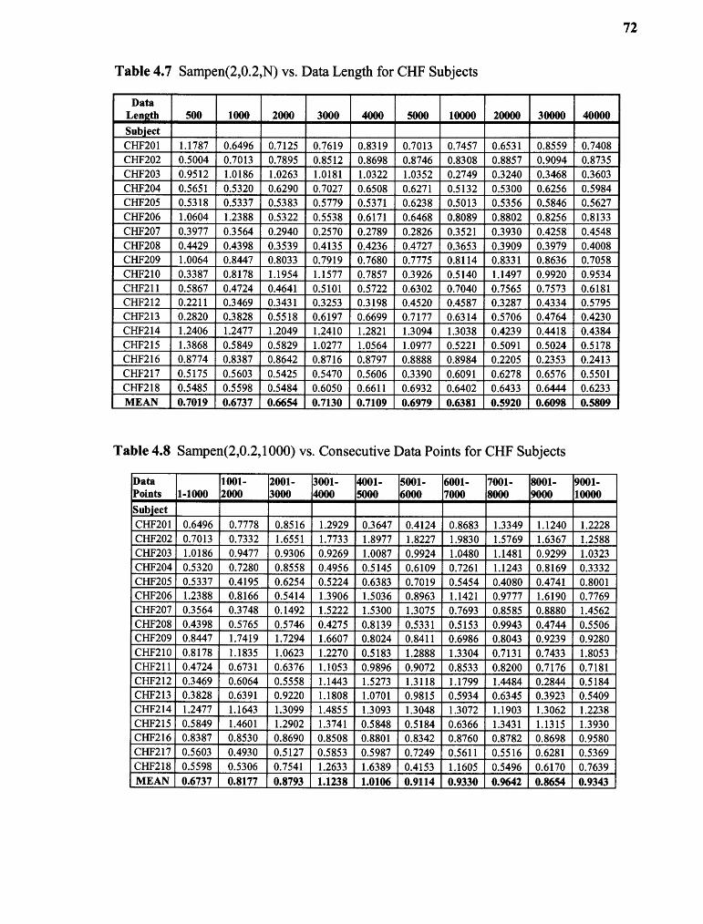
Table 4.7 Sampen(2,0.2,N) vs. Data Length for CHF Subjects
DataLength 500 1000 2000 3000 4000 5000 10000 20000 30000 40000SubjectCHF201 1.1787 0.6496 0.7125 0.7619 0.8319 0.7013 0.7457 0.6531 0.8559 0.7408CHF202 0.5004 0.7013 0.7895 0.8512 0.8698 0.8746 0.8308 0.8857 0.9094 0.8735CHF203 0.9512 1.0186 1.0263 1.0181 1.0322 1.0352 0.2749 0.3240 0.3468 0.3603CHF204 0.5651 0.5320 0.6290 0.7027 0.6508 0.6271 0.5132 0.5300 0.6256 0.5984CHF205 0.5318 0.5337 0.5383 0.5779 0.5371 0.6238 0.5013 0.5356 0.5846 0.5627CHF206 1.0604 1.2388 0.5322 0.5538 0.6171 0.6468 0.8089 0.8802 0.8256 0.8133CHF207 0.3977 0.3564 0.2940 0.2570 0.2789 0.2826 0.3521 0.3930 0.4258 0.4548CHF208 0.4429 0.4398 0.3539 0.4135 0.4236 0.4727 0.3653 0.3909 0.3979 0.4008CHF209 1.0064 0.8447 0.8033 0.7919 0.7680 0.7775 0.8114 0.8331 0.8636 0.7058CHF210 0.3387 0.8178 1.1954 1.1577 0.7857 0.3926 0.5140 1.1497 0.9920 0.9534CHF211 0.5867 0.4724 0.4641 0.5101 0.5722 0.6302 0.7040 0.7565 0.7573 0.6181CHF212 0.2211 0.3469 0.3431 0.3253 0.3198 0.4520 0.4587 0.3287 0.4334 0.5795CHF213 0.2820 0.3828 0.5518 0.6197 0.6699 0.7177 0.6314 0.5706 0.4764 0.4230CHF214 1.2406 1.2477 1.2049 1.2410 1.2821 1.3094 1.3038 0.4239 0.4418 0.4384CHF215 1.3868 0.5849 0.5829 1.0277 1.0564 1.0977 0.5221 0.5091 0.5024 0.5178CHF216 0.8774 0.8387 0.8642 0.8716 0.8797 0.8888 0.8984 0.2205 0.2353 0.2413CHF217 0.5175 0.5603 0.5425 0.5470 0.5606 0.3390 0.6091 0.6278 0.6576 0.5501CHF218 0.5485 0.5598 0.5484 0.6050 0.6611 0.6932 0.6402 0.6433 0.6444 0.6233MEAN 0.7019 0.6737 0.6654 0.7130 0.7109 0.6979 0.6381 0.5920 0.6098 0.5809
Table 4.8 Sampen(2,0.2,1000) vs. Consecutive Data Points for CHF Subjects
DataPoints 1-1000
1001-2000
2001-3000
3001- 4000
4001- 5000
5001-6000
6001-7000
7001- 8000
8001-9000
9001-10000
SubjectCHF201 0.6496 0.7778 0.8516 1.2929 0.3647 0.4124 0.8683 1.3349 1.1240 1.2228CHF202 0.7013 0.7332 1.6551 1.7733 1.8977 1.8227 1.9830 1.5769 1.6367 1.2588CHF203 1.0186 0.9477 0.9306 0.9269 1.0087 0.9924 1.0480 1.1481 0.9299 1.0323CHF204 0.5320 0.7280 0.8558 0.4956 0.5145 0.6109 0.7261 1.1243 0.8169 0.3332CHF205 0.5337 0.4195 0.6254 0.5224 0.6383 0.7019 0.5454 0.4080 0.4741 0.8001CHF206 1.2388 0.8166 0.5414 1.3906 1.5036 0.8963 1.1421 0.9777 1.6190 0.7769CHF207 0.3564 0.3748 0.1492 1.5222 1.5300 1.3075 0.7693 0.8585 0.8880 1.4562CHF208 0.4398 0.5765 0.5746 0.4275 0.8139 0.5331 0.5153 0.9943 0.4744 0.5506CHF209 0.8447 1.7419 1.7294 1.6607 0.8024 0.8411 0.6986 0.8043 0.9239 0.9280CHF210 0.8178 1.1835 1.0623 1.2270 0.5183 1.2888 1.3304 0.7131 0.7433 1.8053CHF211 0.4724 0.6731 0.6376 1.1053 0.9896 0.9072 0.8533 0.8200 0.7176 0.7181CHF212 0.3469 0.6064 0.5558 1.1443 1.5273 1.3118 1.1799 1.4484 0.2844 0.5184CHF213 0.3828 0.6391 0.9220 1.1808 1.0701 0.9815 0.5934 0.6345 0.3923 0.5409CHF214 1.2477 1.1643 1.3099 1.4855 1.3093 1.3048 1.3072 1.1903 1.3062 1.2238CHF215 0.5849 1.4601 1.2902 1.3741 0.5848 0.5184 0.6366 1.3431 1.1315 1.3930CHF216 0.8387 0.8530 0.8690 0.8508 0.8801 0.8342 0.8760 0.8782 0.8698 0.9580CHF217 0.5603 0.4930 0.5127 0.5853 0.5987 0.7249 0.5611 0.5516 0.6281 0.5369CHF218 0.5598 0.5306 0.7541 1.2633 1.6389 0.4153 1.1605 0.5496 0.6170 0.7639MEAN 0.6737 0.8177 0.8793 1.1238 1.0106 0.9114 0.9330 0.9642 0.8654 0.9343
72
73
Tables 4.9 and 4.10 shows the MSE analysis of NSR and CHF subjects,
respectively. They show the Sample entropy values at each scale. As can be seen in Table
4.9, 36 out of a total of 44 NSR subjects have the SampEn(2,0.2,N) > 0.9 for more than
10 scales. As can be seen in Table 4.10, 10 out of a total of 15 CHF subjects have the
SampEn(2,0.2,N) < 0.9 for more than 10 scales. The true positive specificity is 0.81. The
true negative specificity is 0.67. The false positive specificity is 0.33. The false negative
specificity is 0.19.

74
Table 4.9 MSE Analysis for NSR Subjects
Scale 1 2 3 4 5 6 7 8 9 10SubjectNSR001 0.7977 0.9381 0.9331 1.0948 1.1582 1.1757 1.2378 1.2248 1.2570 1.2635NSR002 1.3603 1.0758 1.0811 1.0680 1.1572 1.1959 1.2016 1.2523 1.2437 1.2625NSR003 0.8179 0.8489 0.9650 0.9991 1.0330 1.0967 1.0782 1.0662 1.0864 1.0527NSR004 0.7828 0.8548 0.8532 0.8791 0.8913 0.9281 0.9240 0.9317 0.9367 0.9338NSR005 0.7574 0.5015 0.4952 0.6065 0.6475 0.6724 0.7156 0.7484 0.7569 0.7618NSR006 0.5320 0.6791 0.8189 0.9152 0.9550 0.9772 0.9937 1.0215 1.0372 1.0486NSR007 0.5633 0.6444 0.7611 0.7879 0.8126 0.8030 0.8077 0.7969 0.8070 0.8085NSR008 0.9727 1.0249 1.1312 1.0782 1.1446 1.2005 1.2322 1.2142 1.2417 1.2496NSR009 1.0066 0.9048 1.0727 1.0777 1.1312 1.2430 1.2549 1.3035 1.3289 1.3242NSR010 0.8556 0.8542 0.8602 0.8041 0.9068 0.9735 0.9578 0.9946 1.0230 1.0237NSR011 0.9617 1.0226 1.0244 1.0288 1.0172 1.0351 1.0462 0.9963 0.9982 0.9830NSR012 0.8598 0.7158 0.8941 0.9550 1.0094 1.0860 1.0909 1.0844 1.1211 1.1029NSR013 0.6143 0.4749 0.6032 0.6143 0.6776 0.7247 0.7207 0.7514 0.7551 0.7589NSR014 0.7818 0.8807 1.0189 1.1307 1.2234 1.2899 1.3087 1.3237 1.3354 1.3207NSR015 1.2077 1.3020 1.2595 1.2236 1.3692 1.4347 1.4010 1.4405 1.4671 1.4668NSR016 1.4017 1.0607 1.0873 1.1341 1.1139 1.1534 1.1800 1.1514 1.2019 1.1950NSR017 0.6872 0.5932 0.6235 0.7427 0.7743 0.7919 0.8413 0.8565 0.8707 0.8962NSR018 0.5768 0.6506 0.6664 0.6755 0.6604 0.6565 0.6600 0.6602 0.6475 0.6484NSR019 0.9425 0.7389 0.8346 0.7981 0.8703 0.8802 0.9249 0.9327 0.9668 0.9594NSR020 1.2406 0.8791 0.8917 0.9247 0.9789 1.0692 1.1093 1.1238 1.1318 1.1675NSR021 0.5230 0.4976 0.4853 0.4807 0.5008 0.5403 0.5631 0.5807 0.5882 0.5928NSR022 0.5315 0.7309 0.8085 0.9199 0.9638 0.9817 1.0026 0.9770 0.9759 0.9822NSR023 0.6906 0.8217 0.9209 1.0320 1.1049 1.1159 1.1329 1.1162 1.1239 1.1154NSR024 0.4563 0.4501 0.5170 0.5971 0.6578 0.7047 0.7413 0.7610 0.7871 0.7957NSR025 0.6787 0.9058 1.0114 1.2408 1.3325 1.3661 1.3890 1.3476 1.3445 1.3287NSR026 0.8137 0.9377 0.9923 1.1304 1.2011 1.1847 1.2077 1.2402 1.2111 1.2369NSR027 0.8006 0.9896 1.0534 1.2720 1.3144 1.4198 1.4218 1.4600 1.4430 1.4419NSR028 1.5651 1.0754 1.0100 1.1815 1.3270 1.3601 1.3576 1.4436 1.4381 1.4101NSR029 0.9085 0.7089 0.7211 0.8151 0.8082 0.8170 0.8594 0.8715 0.8765 0.8950NSR030 0.6495 0.5032 0.5456 0.6100 0.6589 0.6876 0.7097 0.7074 0.7255 0.7234NSR031 0.7515 0.6428 0.6896 0.8017 0.8612 0.9378 0.9478 0.9880 0.9981 1.0320NSR032 0.9219 1.0271 0.7955 0.8230 0.7898 0.7812 0.8334 0.8093 0.8412 0.8269NSR033 0.7530 0.8230 0.9257 1.0103 1.0779 1.1293 1.1659 1.1798 1.2116 1.2239NSR034 0.7022 0.6321 0.6813 0.7729 0.8088 0.8535 0.8792 0.9098 0.9035 0.9409NSR035 0.7864 0.6583 0.6979 0.7606 0.8207 0.8989 0.9016 0.9084 0.8966 0.8961NSR036 1.0773 1.0084 0.9495 0.9409 0.9627 0.9920 0.9850 0.9819 0.9871 0.9834NSR037 1.2040 1.2617 1.4493 1.6125 1.6163 1.6016 1.6401 1.6105 1.5898 1.6090NSR038 1.0675 1.4462 1.5801 1.7372 1.8718 1.8296 1.8474 1.8484 1.8141 1.8176NSR039 1.0966 1.2371 1.6181 1.7415 1.7291 1.7121 1.6557 1.6095 1.5762 1.5652NSR040 0.8374 1.0764 1.1378 1.3161 1.3216 1.3650 1.3187 1.3426 1.2879 1.2972NSR041 0.9582 1.0845 1.1040 1.1695 1.1555 1.1929 1.2004 1.2139 1.2193 1.2333NSR042 0.7816 0.7738 0.9521 1.0422 1.0813 1.1472 1.1533 1.1584 1.1669 1.1650NSR043 1.2948 1.4413 1.5502 1.6649 1.6852 1.6427 1.6015 1.6057 1.6098 1.5744NSR044 0.8740 1.2884 1.5579 1.7001 1.7514 1.7599 1.7773 1.7934 1.7946 1.7736MEAN 0.8737 0.8788 0.9461 1.0207 1.0667 1.1002 1.1132 1.1214 1.1278 1.1293

75
Table 4.9 MSE Analysis for NSR Subjects (Continued)
Scale 11 12 13 14 15 16 17 18 19 20SubjectNSR001 1.2532 1.2953 1.2887 1.3024 1.3119 1.3180 1.3037 1.3170 1.3198 1.3285NSR002 1,2634 1.2668 1.2964 1.2824 1.3040 1.2933 1.2756 1.2683 1.2443 1.2747NSR003 1,0655 1.0587 1.0610 1.0158 1.0170 1.0362 1.0117 0.9994 1.0322 1.0045NSR004 0.9321 0.9169 0.9094 0.8980 0.8993 0.8963 0.8744 0.8895 0.8903 0.8674NSR005 0.7892 0.7979 0.7976 0.8243 0.8120 0.8251 0.8270 0.8200 0.8424 0.8383NSR006 1.0444 1.0470 1.0473 1.0602 1.0629 1.0638 7 1.0534 1.0513 1.0596 1.0806NSR007 0.7967 0.8085 0.8075 0.8153 0.7988 0.8129 0.8141 0.7988 0.8088 0.8153NSR008 1.2613 1.2527 1.2705 1.2889 1.2734 1.2739 1.2767 1.2634 1.2791 1.2732NSR009 1.3665 1.3761 1.3882 1.4052 1.3781 1.4016 1.4207 1.4250 1.4259 1.4121NSR010 1.0274 1.0374 1.0456 1.0536 1.0534 1.0488 1.0384 1.0475 1.0347 1.0244NSR011 0,9968 0.9590 0.9562 0.9487 0.9459 0.9275 0.9503 0.9473 0.9503 0.9165NSR012 1.1012 1.1163 1.1058 1.0980 1.1312 1.0990 1.1201 1.1415 1.1411 1.1583NSR013 0.7557 0.7796 0.7692 0.7693 0.7702 0.7882 0.7803 0.7838 0.8077 0.7913NSR014 1.2992 1.3098 1.2955 1.3080 1.3033 1.2710 1.3055 1.2751 1.2904 1.2991NSR015 1.4918 1.4911 1.5107 1.5027 1.5154 1.4934 1.4910 1.5160 1.4976 1.5156NSR016 1.1920 1.2351 1.2470 1.2226 1.2644 1.2459 1.2561 1.2748 1.2671 1.2694NSR017 0.9042 0.9184 0.9179 0.9360 0.9554 0.9438 0.9573 0.9660 0.9750 0.9759NSR018 0.6530 0.6504 0.6401 0.6486 0.6444 0.6487 0.6691 0.6560 0.6649 0.6601NSR019 0.9622 0.9639 0.9590 0.9506 0.9632 0.9572 0.9592 0.9511 0.9644 0.9728NSR020 1.1948 1.1856 1.2186 1.2308 1.2488 1.2757 1.2793 1.2995 1.2998 1.2989NSR021 0.5998 0.6019 0.6074 0.6145 0.6179 0.6144 0.6254 0.6206 0.6224 0.6305NSR022 0.9800 0.9751 0.9741 0.9734 0.9605 0.9488 0.9564 0.9466 0.9508 0.9379NSR023 1.1058 1.1153 1.1066 1.0962 1.1072 1.1061 1.1308 1.1182 1.0954 1.1207NSR024 0.8104 0.8192 0.8337 0.8536 0.8572 0.8524 0.8734 0.8611 0.8775 0.8894NSR025 1.3134 1.2832 1.2956 1.2526 1.3030 1.2301 1.2379 1.2304 1.2131 1.2302NSR026 1.2445 1.2180 1.2435 1.2466 1.2321 1.2130 1.2125 1.1963 1.2023 1.1654NSR027 1.4370 1.4580 1.4370 1.4178 1.4167 1.4335 1.4225 1.4212 1.4495 1.4202NSR028 1.3768 1.3881 1.3742 1.3747 1.3572 1.3387 1.3278 1.3393 1.3460 1.3247NSR029 0.8729 0.9036 0.9189 0.9068 0.9030 0.9148 0.9314 0.9193 0.9114 0.9035NSR030 0.7245 0.7180 0.7291 0.7299 0.7233 0.7265 0.7193 0.7127 0.7087 0.7127NSR031 1.0353 1.0572 1.0442 1.0724 1.0735 1.0768 1.0732 1.0929 1.0923 1.0877NSR032 0.8351 0.8239 0.8122 0.8211 0.8216 0.7931 0.8148 0.8017 0.7873 0.7706NSR033 1.2287 1.2555 1.2474 1.2542 1.2930 1.2785 1.2617 1.3030 1.2852 1.3255NSR034 0.9260 0.9434 0.9247 0.9295 0.9312 0.9316 0.9138 0.9210 0.9154 0.9115NSR035 0.9072 0.8892 0.8910 0.8736 0.8678 0.8365 0.8522 0.8569 0.8488 0.8349NSR036 0.9729 0.9610 0.9680 0.9468 0.9342 0.9501 0.9322 0.9246 0.9061 0.8862NSR037 1.6014 1.5922 1.5975 1.6123 1.5907 1.6028 1.6441 1.6196 1.6295 1.6275NSR038 1.8068 1.7527 1.7412 1.7476 1.7470 1.7021 1.7030 1.7190 1.6843 1.7110NSR039 1.5334 1.5280 1.4923 1.4799 1.4944 1.4998 1.5081 1.4964 1.5196 1.5288NSR040 1.2721 1.2754 1.2413 1.2614 1.2562 1.2558 1.2578 1.2598 1.2536 1.2416NSR041 1.2344 1.2335 1.2769 1.2787 1.2931 1.3105 1.3097 1.3083 1.3362 1.3467NSR042 1.1747 1.1818 1.1949 1.1817 1.2073 1.2231 1.2137 1.2194 1.2309 1.2487NSR043 1.5725 1.5482 1.5447 1.5273 1.5295 1.5498 1.5531 1.5600 1.5401 1.5158NSR044 1.7676 1.7679 1.7326 1.7550 1.7685 1.7517 1.7112 1.7375 1.7349 1.7483MEAN 1.1292 1.1308 1.1309 1.1311 1.1350 1.1309 1.1330 1.1336 1.1349 1.1340

76
Table 4.10 MSE Analysis for CHF Subjects
Scale 1 2 3 4 5 6 7 8 9 10SubjectCHF201 1.1927 0.3910 0.2322 0.2033 0.1957 0.2271 0.2354 0.2540 0.2582 0.2676CHF202 0.7213 0.5460 0.6490 0.5809 0.6586 0.6207 0.6324 0.5944 0.6328 0.6061CHF203 0.7414 0.6630 0.6483 0.6286 0.5970 0.5425 0.5266 0.5236 0.5281 0.5258CHF204 0.6621 0.7187 0.8695 0.8625 0.9587 0.9403 0.9974 0.9819 0.9365 0.9833CHF205 1.3701 0.7916 0.6458 0.5294 0.5001 0.4706 0.4457 0.4364 0.4474 0.4638CHF206 0.4548 0.4954 0.5838 0.6831 0.7526 0.8011. 0.8324 0.8559 0.8760 0.8925CHF207 0.6885 0.5370 0.5742 0.6635 0.7365 0.7818 0.8282 0.8570 0.8717 0.9060CHF208 0.7671 0.9256 1.0627 1.0584 1.0481 1.0362 1.0119 0.9956 0.9748 0.9744CHF209 0.5795 0.6233 0.5709 0.5895 0.6547 0.6960 0.7363 0.7938 0.8160 0.8254CHF210 0.7350 0.5940 0.6047 0.6466 0.6534 0.7071 0.7562 0.8079 0.8141 0.8219CHF211 0.4384 0.4040 0.4707 0.5079 0.5473 0.5725 0.6183 0.6613 0.6783 0.7116CHF212 1.4409 0.8815 0.8174 0.8350 0.8820 0.9348 0.9821 1.0892 1.1204 1.1419CHF213 0.9583 0.4350 0.3899 0.4069 0.4275 0.4580 0.4778 0.5438 0.5679 0.5766CHF214 0.6715 0.6685 0.5454 0.6094 0.6067 0.6058 0.6260 0.6451 0.6740 0.6538CHF215 0.6233 0.5549 0.6077 0.6608 0.7095 0.7357 0.7422 0.7952 0.8382 0.8746MEAN 0.8030 0.6153 0.6181 0.6311 0.6619 0.6753 0.6966 0.7223 0.7356 0.7484
Table 4.10 MSE Analysis for CHF Subjects (Continued)
Scale 11 12 13 14 15 16 17 18 19 20SubjectCHF201 0.2881 0.3049 0.3188 0.3284 0.3376 0.3518 0.3629 0.3737 0.3763 0.3842CHF202 0.6010 0.5669 0.5781 0.5838 0.5992 0.5809 0.5910 0.5865 0.5732 0.5723CHF203 0.5270 0.5322 0.5527 0.5346 0.5478 0.5711 0.5808 0.5882 0.5860 0.5983CHF204 0.9630 0.9694 0.9509 0.9787 0.9736 0.9638 0.9686 0.9683 0.9703 0.9538CHF205 0.4475 0.4707 0.4580 0.4683 0.4969 0.4900 0.4994 0.4921 0.5208 0.5169CHF206 0.9028 0.8994 0.9221 0.9253 0.9463 0.9528 0.9594 0.9767 0.9752 0.9913CHF207 0.9293 0.9155 0.9457 0.9572 0.9504 0.9833 0.9735 0.9612 1.0011 0.9754CHF208 0.9676 0.9694 0.9312 0.9267 0.9132 0.9293 0.9152 0.9078 0.9066 0.8894CHF209 0.8614 0.8781 0.8907 0.9100 0.9114 0.9257 0.9198_ 0.9470 0.9313 0.9374CHF210 0.8274 0.8438 0.8345 0.8511 0.8595 0.8598 0.8817 0.8568 0.8569 0.8659CHF211 0.7247 0.7502 0.7680 0.7828 0.8079 0.8288 0.8339 0.8528 0.8629 0.8775CHF212 1.1539 1.1726 1.1751 1.1767 1.1873 1.1990 1.2217 1.2192 1.2112 1.2235CHF213 0.5986 0.5991 0.6128 0.6140 0.6313 0.6549 0.6553 0.6505 0.6543 0.6711CHF214 0.6674 0.6611 0.6561 0.6790 0.6889 0.6680 0.6701 0.6955 0.6709 0.6696CHF215 0.8994 0.9287 0.9550 0.9623 0.9914 1.0256 1.0388 1.0588 1.0813 1.1012MEAN 0.7573 0.7641 0.7700 0.7786 0.7895 0.7990 0.8048 0.8090 0.8119 0.8152

77
Figures 4.1 and 4.2 show SampEn as a function of tolerance factor r and pattern
length m, respectively. One can see that as tolerance factor r increases the value of
SampEn decreases. Also as pattern length m increases the value of SampEn decreases.
This is in accordance with the theory. As r and m increases, the number of matches
increases. This results in a lower value of the sample entropy.
Figure 4.1 SampEn (m,r,1000) vs. r for different m for NSR group.

78
Figure 4.2 SampEn (m,r,1000) vs. m for different r for NSR group.
Figures 4.3 and 4.4 show the variation in the values of ApEn and SampEn with
time for NSR and CHF group. As seen in the figure, the values of ApEn and SampEn are
higher for the NSR group than the CHF group for the first thousand data points.
However, values do not remain high for all other thousand data points. This shows that
the underlying dynamics of the time series varies with time. This variation in the
underlying dynamics could be due to intrinsic factors (circadian rhythm, baroreceptor
reflex, etc.) or extrinsic factors (walking, exercise, etc.).
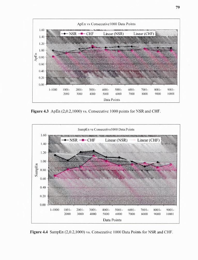
79
Figure 4.3 ApEn (2,0.2,1000) vs. Consecutive 1000 points for NSR and CHF.
Figure 4.4 SampEn (2,0.2,1000) vs. Consecutive 1000 Data Points for NSR and CHF.

80
4.5 t —Test Analysis
The t-test is the most commonly used parametric test to evaluate the difference in means
between two groups. The p-level reported with the t-test represents the probability of
error associated with rejecting the hypothesis of no difference between the two groups
when, in fact, the hypothesis is true [42]. Both one tail and two tail t-tests are used for our
analysis. In using the t-test one makes the assumption that both samples are drawn from
independent populations that can be described by a normal distribution, and that the
observations are independent random variables [43]. The t-test is used to compare the
mean entropy measures for NSR and CHF subjects. The null hypothesis is that the means
of the entropy measures are not different. The alternative hypothesis is that the means of
the entropy measures are different. If |t0| > t critical, one would reject the null hypothesis
and conclude that the means of entropy measures are different. This can also be tested
using P value. The null hypothesis is rejected for P < 0.05.
Table 4.11 t-Test for ApEn(2,0.2,1000) of NSR and CHF Subjects
t-Test for ApEn of NSR and CHFNSR CHF
Mean 0.9945 0.8157Variance 0.0440 0.0547
Observations 44.0000 18.0000Hypothesized Mean Difference 0.0000
Df 29.0000t Stat 2.8123
P(T<=t) one-tail 0.0044t Critical one-tail 1.6991P(T<=t) two-tail 0.0087t Critical two-tail 2.0452
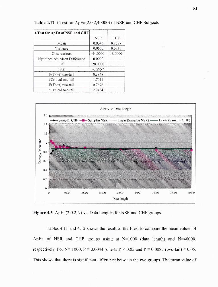
Table 4.12 t-Test for ApEn(2,0.2,40000) of NSR and CHF Subjects
t-Test for ApEn of NSR and CHFNSR CHF
Mean 0.8346 0,8587Variance 0.0670 0.0931
Observations 44.0000 18.0000Hypothesized Mean Difference 0.0000
Df 28.0000t Stat -0.2957
P(T<=t) one-tail 0.3848t Critical one-tail 1,7011P(T<=t) two-tail 0.7696t Critical two-tail 2.0484
81
Figure 4.5 ApEn(2,0.2,N) vs. Data Lengths for NSR and CHF groups.
Tables 4.11 and 4.12 shows the result of the t-test to compare the mean values of
ApEn of NSR and CHF groups using at N=1000 (data length) and N=40000,
respectively. For N= 1000, P = 0.0044 (one-tail) < 0.05 and P = 0.0087 (two-tail) < 0.05.
This shows that there is significant difference between the two groups. The mean value of
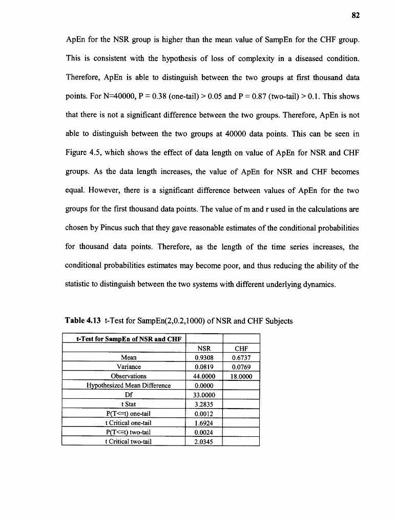
82
ApEn for the NSR group is higher than the mean value of SampEn for the CHF group.
This is consistent with the hypothesis of loss of complexity in a diseased condition.
Therefore, ApEn is able to distinguish between the two groups at first thousand data
points. For N=40000, P = 0.38 (one-tail) > 0.05 and P = 0.87 (two-tail) > 0.1. This shows
that there is not a significant difference between the two groups. Therefore, ApEn is not
able to distinguish between the two groups at 40000 data points. This can be seen in
Figure 4.5, which shows the effect of data length on value of ApEn for NSR and CHF
groups. As the data length increases, the value of ApEn for NSR and CHF becomes
equal. However, there is a significant difference between values of ApEn for the two
groups for the first thousand data points. The value of m and r used in the calculations are
chosen by Pincus such that they gave reasonable estimates of the conditional probabilities
for thousand data points. Therefore, as the length of the time series increases, the
conditional probabilities estimates may become poor, and thus reducing the ability of the
statistic to distinguish between the two systems with different underlying dynamics.
Table 4.13 t-Test for SampEn(2,0.2,1000) of NSR and CHF Subjects
t-Test for SampEn of NSR and CHFNSR CHF
Mean 0.9308 0.6737Variance 0.0819 0.0769
Observations 44.0000 18.0000Hypothesized Mean Difference 0.0000
Df 33.0000t Stat 3.2835
P(T<=t) one-tail 0.0012t Critical one-tail 1.6924P(T<=t) two-tail 0.0024t Critical two-tail 2.0345

Table 4.14 t-Test for Sampen of NSR and CHF for 40000 Data Points
t-Test for SampEn of NSR and CHFNSR CHF
Mean 0.6683 0.5809Variance 0.0478 0.0345
Observations 44.0000 18.0000Hypothesized Mean Difference 0.0000
Df 37.0000t Stat 1.5968
P(T<=t) one-tail 0.0594t Critical one-tail 1.6871P(T<=t) two-tail 0.1188t Critical two-tail 2.0262
83
Figure 4.6 SampEn vs. Data Lengths for NSR and CHF.
Tables 4.13 and 4.14 show the results of the t-test to compare the mean values of
SampEn of NSR and CHF groups using N=1000 (data length) and N=40000,
respectively. For N= 1000, P = 0.0012 (one-tail) < 0.05 and P = 0.0024 (two-tail) < 0.1.
This shows that there is significant difference between the two groups. The mean value of

84
the SampEn for the NSR group is higher than the mean value of the SampEn for the CHF
group. This is consistent with the hypothesis of loss of complexity in a diseased
condition. Therefore, SampEn is able to distinguish between the two groups at 1000 data
points. For N=40000, P = 0.059 (one-tail) > 0.05 and P = 0.1187 (two-tail) > 0.1. This
shows that there is not a significant difference between the two groups. Therefore,
SampEn is not able to distinguish between the two groups at 40000 data points. This can
be seen in Figure 4.6, which shows the effect of data length on value of SampEn for NSR
and CHF groups. As the data length increases, the value of SampEn for NSR and CHF
becomes equal. However, there is a significant difference between values of SampEn for
the two groups for the first thousand data points. The value of m and r used in the
calculations are chosen by Pincus such that they gave reasonable estimates of the
conditional probabilities for thousand data points. Therefore, as the length of the time
series increases, the conditional probabilities estimates may become poor, and thus
reducing the ability of the statistic to distinguish between the two systems with different
underlying dynamics.
4.6 ANOVA Analysis
The analysis of variance (ANOVA) is the most commonly used and appropriate
procedure to test the over all effect of the treatments (in our case various activities) on the
experiment (in our case the entropy of the RR interval time series of the subjects). In any
experiment, variability arising from a nuisance factor can affect the results. A nuisance
factor is a design factor that probably has an effect on the response, but one are not
interested in that effect. In our case the nuisance factor is the subject. The effect of
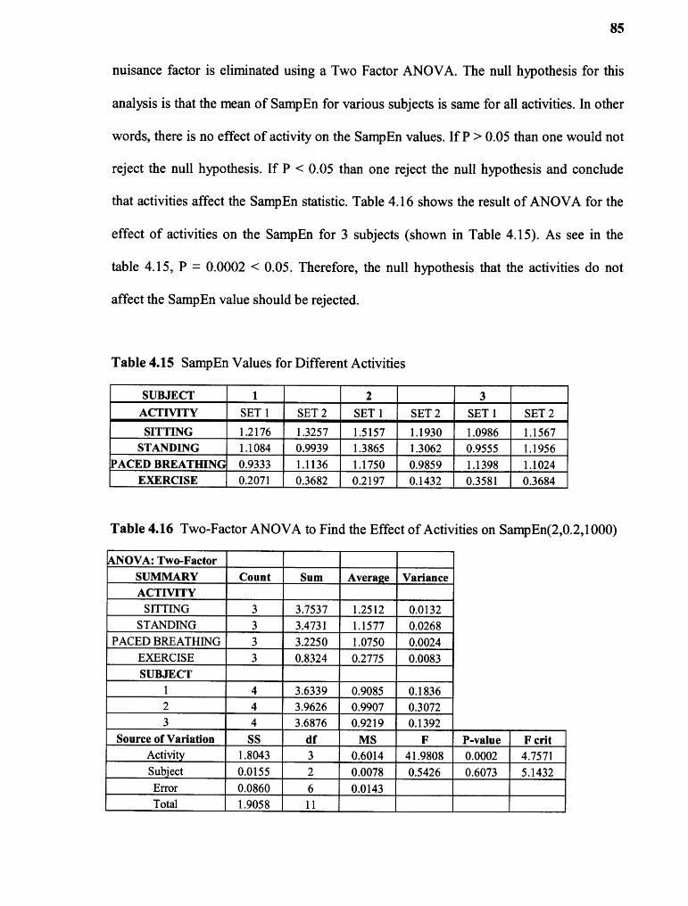
85
nuisance factor is eliminated using a Two Factor ANOVA. The null hypothesis for this
analysis is that the mean of SampEn for various subjects is same for all activities. In other
words, there is no effect of activity on the SampEn values. If P > 0.05 than one would not
reject the null hypothesis. If P < 0.05 than one reject the null hypothesis and conclude
that activities affect the SampEn statistic. Table 4.16 shows the result of ANOVA for the
effect of activities on the SampEn for 3 subjects (shown in Table 4.15). As see in the
table 4.15, P = 0.0002 < 0.05. Therefore, the null hypothesis that the activities do not
affect the SampEn value should be rejected.
Table 4.15 SampEn Values for Different Activities
SUBJECT 1 2 3ACTIVITY SET 1 SET 2 SET 1 SET 2 SET 1 SET 2
SITTING 1.2176 1.3257 1.5157 1.1930 1.0986 1.1567STANDING 1.1084 0.9939 1.3865 1.3062 0.9555 1.1956
PACED BREATHING 0.9333 1.1136 1.1750 0.9859 1.1398 1.1024EXERCISE 0.2071 0.3682 0.2197 0.1432 0.3581 0.3684
Table 4.16 Two-Factor ANOVA to Find the Effect of Activities on SampEn(2,0.2,1000)
ANOVA: Two-FactorSUMMARY Count Sum Average VarianceACTIVITY
SITTING 3 3.7537 1.2512 0.0132STANDING 3 3.4731 1.1577 0.0268
PACED BREATHING 3 3.2250 1.0750 0.0024EXERCISE 3 0.8324 0.2775 0.0083SUBJECT
1 4 3.6339 0.9085 0.18362 4 3.9626 0.9907 0.30723 4 3.6876 0.9219 0.1392
Source of Variation SS df MS F P-value F critActivity 1.8043 3 0.6014 41.9808 0.0002 4.7571Subject 0.0155 2 0.0078 0.5426 0.6073 5.1432Error 0.0860 6 0.0143Total 1.9058 11

86
Tables 4.17, 4.18, 4.19, 4.20, 4.21 and 4.22 shows the result of ANOVA to
compare the means of SampEn during Sitting and Standing, Sitting and Paced Breathing,
Sitting and Exercise, Standing and Paced Breathing, Standing and Exercise, and Paced
Breathing and Exercise, respectively.
Table 4.17 ANOVA for Sitting vs. Standing Activity
ANOVA: Two-FactorSUMMARY Count Sum Average VarianceACTIVITY
SITTING 3 3.7537 1.2512 0.0132STANDING 3 3.4731 1.1577 0.0268SUBJECT
1 2 2.3228 1.1614 0.02432 2 2.7007 1.3504 0.00003 2 2.2032 1.1016 0.0014
Source of Variation SS df MS F P-value F critActivity 0.0131 1 0.0131 2.0868 0.2854 18.5128Subject 0.0674 2 0.0337 5.3621 0.1572 19.0000Error 0.0126 2 0.0063Total 0.0931 5
Table 4.18 ANOVA for Sitting vs. Paced Breathing Activity
ANOVA: Two-FactorSUMMARY Count Sum Average VarianceACTIVITY
SITTING 3 3.7537 1.2512 0.0132PACED BREATHING 3 3.2250 1.0750 0.0024
SUBJECT1 2 2.2951 1.1476 0.03082 2 2.4348 1.2174 0.03753 2 2.2488 1.1244 0.0000
Source of Variation SS df MS F P-value F critActivity 0.0466 1 0.0466 4.2821 0.1744 18.5128Subject 0.0094 2 0.0047 0.4312 0.6987 19.0000Error 0.0218 2 0.0109Total 0.0777 5

Table 4.19 ANOVA for Sitting vs. Exercise Activity
ANOVA: Two-FactorSUMMARY Count Sum Average VarianceACTIVITY
SITTING 3 3.7537 1.2512 0.0132EXERCISE 3 0.8324 0.2775 0.0083SUBJECT
1 2 1.5593 0.7797 0.48412 2 1.5358 0.7679 0.68783 2 1.4909 0.7455 0.2922
Source of Variation SS df MS F P-value F critActivity 1.4223 1 1.4223 68.0597 0.0144 18.5128Subject 0.0012 2 0.0006 0.0289 0.9719 19.0000Error 0.0418 2 0.0209Total 1.4653 5
Table 4.20 ANOVA for Standing vs. Paced Breathing Activity
ANOVA: Two-FactorSUMMARY Count Sum Average VarianceACTIVITYSTANDING 3 3.4731 1.1577 0.0268
PACED BREATHING 3 3.2250 1.0750 0.0024SUBJECT
1 2 2.0746 1.0373 0.00042 2 2.4268 1.2134 0.03543 2 2.1967 1.0983 0.0010
Source of Variation SS df MS F P-value F critActivity 0.0103 1 0.0103 0.7734 0.4719 18.5128Subject 0.0320 2 0.0160 1.2062 0.4533 19.0000Error 0.0265 2 0.0133Total 0.0688 5
87
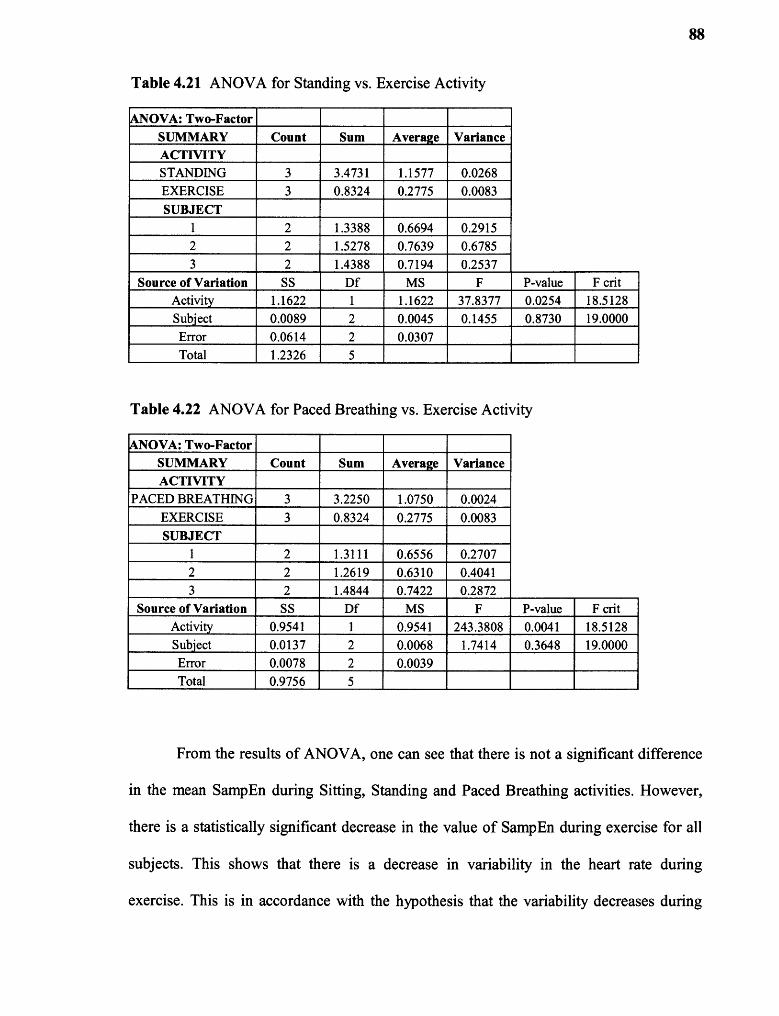
88
Table 4.21 ANOVA for Standing vs. Exercise Activity
ANOVA: Two-FactorSUMMARY Count Sum Average VarianceACTIVITYSTANDING 3 3.4731 1.1577 0.0268EXERCISE 3 0.8324 0.2775 0.0083SUBJECT
1 2 1.3388 0.6694 0.29152 2 1.5278 0.7639 0.67853 2 1.4388 0.7194 0.2537
Source of Variation SS Df MS F P-value F critActivity 1.1622 1 1.1622 37.8377 0.0254 18.5128Subject 0.0089 2 0.0045 0.1455 0.8730 19.0000Error 0.0614 2 0.0307Total 1.2326 5
Table 4.22 ANOVA for Paced Breathing vs. Exercise Activity
ANOVA: Two-FactorSUMMARY Count Sum Average VarianceACTIVITY
PACED BREATHING 3 3.2250 1.0750 0.0024EXERCISE 3 0.8324 0.2775 0.0083SUBJECT
1 2 1.3111 0.6556 0.27072 2 1.2619 0.6310 0.40413 2 1.4844 0.7422 0.2872
Source of Variation SS Df MS F P-value F critActivity 0.9541 1 0.9541 243.3808 0.0041 18.5128Subject 0.0137 2 0.0068 1.7414 0.3648 19.0000Error 0.0078 2 0.0039Total 0.9756 5
From the results of ANOVA, one can see that there is not a significant difference
in the mean SampEn during Sitting, Standing and Paced Breathing activities. However,
there is a statistically significant decrease in the value of SampEn during exercise for all
subjects. This shows that there is a decrease in variability in the heart rate during
exercise. This is in accordance with the hypothesis that the variability decreases during
89
the exercise. Exercise is a stressful condition. This causes the control of the sympathetic
nervous system to be more dominant than the control of the parasympathetic nervous
system. This can be viewed as a decrease in the interaction between the two systems and
thus reduces the variability in the heart rate.
4.7 MSE Analysis
Figure 4.7 shows the MSE analysis of RR interval time series derived from NSR and
CHF group. For scale one the SampEn entropy is not able to distinguish between the
NSR and CHF group. But as the scale increases, the NSR group has significantly (p = 0
as seen in Table 4.23) higher values than the CHF group. This shows that healthy
dynamics are more complex at different scales. The strongest separation between the two
groups is obtained at scale six. The SampEn value for the NSR group increases on small
time scales and then stabilizes to a constant value. The SampEn values for CHF decreases
down to time scale two and then progressively increases. This suggests that for the CHF
group the control mechanisms regulating heart rate on relatively short time scales are the
most affected [41].
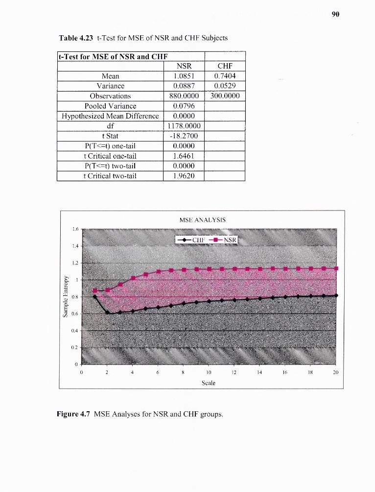
Table 4.23 t-Test for MSE of NSR and CHF Subjects
t-Test for MSE of NSR and CHFNSR CHF
Mean 1.0851 0.7404Variance 0.0887 0.0529
Observations 880.0000 300.0000Pooled Variance 0.0796
Hypothesized Mean Difference 0.0000df 1178.0000
t Stat -18.2700P(T<=t) one-tail 0.0000t Critical one-tail 1.6461P(T<=t) two-tail 0.0000t Critical two-tail 1.9620
90
Figure 4.7 MSE Analyses for NSR and CHF groups.

CHAPTER 5
CONCLUSIONS AND FUTURE WORK
5.1 Conclusions and Future Work
In conclusion, the goal of this thesis was to study the heart rate variability using entropy
measures namely, ApEn, SampEn and MSE. ApEn (2,0.2,1000) was found to be 0.99 ±
0.21 (mean ± standard deviation) for the NSR group and 0.82 ± .23 for the CHF group for
the first thousand RR intervals. SampEn (2,0.2,1000) was found to be 0.93 ± 0.28 for
NSR group and 0.67 ± .27 for CHF group for the first thousand RR intervals. The value
of ApEn and SampEn statistics were higher in the NSR group than the CHF group. This
is in accordance with the hypothesis that there is loss of complexity in RR interval time
series in diseased conditions. The difference in the value of ApEn and SampEn statistics
for the NSR group and the CHF group were statistically significant for N = 1000.
However, the difference was not statistically significant for N = 40000. The value of
ApEn for the NSR and the CHF group became equal for larger data lengths. However,
the SampEn value remained consistently higher for NSR group than CHF group for all
data lengths tested, suggesting that SampEn is a better statistic than ApEn. The
magnitude of ApEn and SampEn varied with time for both the groups. Also, the
magnitude of ApEn and SampEn did not remain high for the NSR group than the CHF
group for each thousand RR intervals in the time series. As the activity during data
acquisition is not known, this change could not be correlated with activity of the subjects.
This variation in entropy measures with time can be attributed to the non-stationarity of
the data resulting from the change in underlying cardiac dynamics because of either
91
92
intrinsic or extrinsic factors or both. A detailed study is required to find the effect on non-
stationarity in time series on the entropy measures. The statistic ApEn (2,0.2,1000) was
able to correctly identify 27 subjects out of a total of 44 subjects in the NSR group as
NSR subjects and 12 subjects out of a total of 18 subjects in the CHF group as CHF
subjects, assuming that ApEn (2,0.2,1000) > 0.9 indicates normal conditions. The statistic
SampEn (2,0.2,1000) was able to correctly identify 27 subjects out of a total of 44
subjects in the NSR group as NSR subjects and 12 subjects out of a total of 18 subjects in
the CHF group as CHF subject, assuming that SampEn (2,0.2,1000) > 0.8 indicates
normal conditions. The true positive specificity for ApEn and SampEn statistics is found
to be 0.61. The true negative specificity for ApEn and SampEn statistics is found to be
0.67.
Effect of various activities namely, sitting on a chair, standing, paced breathing
and exercise on SampEn was studied. The results of the analysis suggest that there is
significant reduction in the value of SampEn (2,0.2,1000) during exercise. This can be
attributed to the fact that the variation in the heart rate decreases during exercise. There is
no significant difference in the value of SampEn for other activities. However, a more
detailed study needs to be done to find the effect of various activities on these statistics as
the number of subjects was very small and precise control of paced breathing was not
verified using power spectrum analysis.
MSE analysis revealed that the SampEn was consistently higher for the NSR
group than the CHF group at higher scales. This is consistent with the hypothesis of loss
of complexity in diseased conditions. The strongest separation occurs at scale 6 and
weakest separation occurs at scale 1. Therefore, not only the specific values of the

93
entropy measure but also their dependence on different scale needs to be taken into
account to distinguish [41] the underlying cardiac dynamics in the NSR and the CHF
group. We are correctly able to identify 36 subjects out of a total of 44 subjects in NSR
group as NSR subjects and 10 subjects out of a total of 15 subjects in CHF group as CHF
subject. The true positive specificity for MSE statistic is found to be 0.81. The true
negative specificity for MSE statistic is found to be 0.67.
Out of the three entropy measures studied, MSE gave the most separability than
the others in classifying the subjects into the NSR and the CHF group. A decrease in
entropy was observed in the CHF group. The lower values of ApEn in the heart failure
population corresponded with previous findings of a reduced complexity (Kaplan et al.,
1991; Kleiger et al., 1987; Pincus et al., 1993; Pincus and Viscarello, 1992; Lin et al.,
2001) in pathologies. However, the findings were contradictory with previous findings of
increased ApEn in CHF by Beckers et al., 2001. Therefore, we can conclude that MSE
and SampEn can be used as a marker of a diseased condition. However, they should be
complemented by other measures. All these measures require at least 1000 data points (—
15 minutes of data). Therefore, these measures cannot be used on very short time series.
Although these results are promising in that they suggest a decrease in entropy in
diseased conditions like CHF, they add little to the understanding of cardiac dynamics.
This study should be performed for a variety of population like subjects with myocardial
infarction, fibrillation, etc. to see the change in entropy for different underlying cardiac
dynamics and hence have a better understanding of the cardiac dynamics. Also, the study
should be performed to determine the entropy measures in populations grouped on the
basis of age and gender. Furthermore, the study should be performed to examine the

94
ability of these methods to detect the onset of disease conditions in subjects. A study
should be performed to examine the ability of these entropy measures to detect the effect
of medication and therapy on diseased population.

APPENDIX A
HENON ATTRACTOR
This appendix describes the Henon attractor used in Chapter 3. The Henon attractor is an
interesting iterated fractal. It consists of two X and Y equations that produce a fractal.
The equations are:
xn = yn-1 + 1 -a*(xn-1)2 (A.1)
yn = b*Xn-1 (A.2)
The default parameters are a = 1.4 and b = 0.3. Figure A.1 shows the Henon attractor for
the default parameters. [44].
Figure A.1 Henon Attractor [44].
95

APPENDIX B
PROGRAMS FOR THE STUDY
This appendix describes the programs used in the study. The programs are written in
MATLAB 7.0. Program A was used to deglitch the RR interval time series. Program B
was used to calculate the Approximate Entropy of the time series. Program C was used to
calculate the Sample Entropy of the time series. Program D was used to calculate the
Multiscale Entropy of the time series. Various functions called in the program are
provided at the end of each main program. Input to each of the main program is a text file
with RR intervals arranged in a column.
Program A: To deglitch the RR interval time series
function datum=deglitching(vals)[a,b]=size(vals);
times(1)=vals(1);for i=2:a
times(i)=times(i-1)+vals(i);endlabels=ones(a,b);[labs,resids] = ardeglch(vals, labels);
c=1;for i=1:a
if labs(i)==1datum(c,1)=vals(i);
c=c+1;endend
function [labs,resids] = ardeglch(data, inlabels, modelorder, iqrcrit)% labs = arresid(data, inlabels, modelorder, iqrcrit)% identifies outliers in a time series by% looking at the residuals of a forward and% backward AR fit.% Excludes from the fit beats labeled 0 in <inlabels>% iqrcrit gives the criteria in inter-quartile range units
% for an outlier.
96

% or from the AR fit.% [labs,resids] = ardegich...% gives the actual values of the residuals as an optional second argument
if nargin < 3modelorder = 3;
endif nargin < 4
iqrcrit = 3.5;end% fit the forward modellabforward = arresid(data, inlabels, modelorder);% fit the backward modellabbackward = arresid( data((length(data)):-1:1), inlabels((length(data)):-1:1), modelorder);% take the smaller of the two residuals, remembering% to put labbackward back in forward order.labels = min(labforward, labbackward(length(data):-1:1) );resids = labels;% Compute the interquartile range and limits for outliers.lims = prctile(labels,[25 50 75]);iqrange = lims(3) - lims(1);bottom = lims(1) - iqrange*iqrcrit;top = lims(3) + iqrange*iqrcrit;% bogus points are marked as 666666 in <labels> or as 0 in <inlabels>labs = (labels > bottom & labels < top & labels —= 666666 & inlabels ~= 0 );
function resids = arresid(data, inlabels, modelorder)% res = arresid(data, inlabels, modelorder, outcrit)% Identifies outliers in a time series by looking% for outliers to a linear prediction model% data -- the time series% inlabels -- a zero for each already-known bogus data item% modelorder -- what model order to use% returns resids --- the residuals written in terms of IQRs from the median% These are synchronized to the data point being predicted.% Convert to a column formatdata = data(:);inlabels = inlabels(:);if length(inlabels) ~= length(data)
error('arresid: data and labels must be the same length.');end% create a lag-embedded matrix of preimagespre = ones( length(data) - modelorder, modelorder+1);Ipre = ones( length(data) - modelorder, modelorder+1);% and the images of thistargs = data( (modelorder+1):(length(data)) );% fill in the matrixfor k=1:modelorder
foo = length(data) - modelorder;pre(:,(k+1)) = data( (modelorder+1-k):(length(data)-k) );Ipre(:,(k+1)) = inlabels( (modelorder+1-k):(length(data)-k) );
endIpre(:,1) = inlabels( (modelorder+1):(length(data)) );% note that the matrix <pre> has all ones in the first column,% to handle the constant part of the linear model% the <Ipre> matrix gives the labels of the correspond entries
97

% in <pre>% get rid of the known bad beats% by identifying any row with a bad beatgoodrows = find( all((lpre—= 0)' )');% The following is for version 5%goodrows = find( all((lpre~= 0),2) );% create matrices for the preimages and targets that have% only clean beatscleanpre = pre(goodrows,:);cleantargs = targs(goodrows);% fit the linear modelparams = cleanpre\cleantargs;% calculate the residualsres = targs - pre*params;% set the output to give the residual for the beat being% predicted. Make bogus residuals big so they% are easily pulled out% Magic number 666666 is used in other programsresids = 666666*ones(size(data));resids( (modelorder + 1):(length(data)) ) = res;
Program B: To calculate the approximate entropy of the RR interval time series.
function approximateentropy(dataset)val=dataset;[a b]= size(val);modelorder=3;inlabels=ones(size(val));[labs,resids] = ardeglch(val, inlabels, modelorder);vvv=find((labs==1));vall=val(vvv);disp('mean and std');disp(mean(vall));disp(std(vall));[a b]=size(vall);vals=vall;%((a-900):(a-99));[c d]=size(vals);times(1,1)=vals(1,1);for i=2:c
times(i,1)=times(i-1,1)+vals(i,1);endilabels=ones(size(vals));rstd = 0.2;%APEN PROG "APENHR" USES R=RSTD*STDDEVIATIONlag = 1;[ntimes,entro,lab]=apenhr(times,vals,ilabels,[rstd,lag]);end
function [t,v,lab] = apenhr(times,vals,labels,params)% [t,v,lab] = apenhr(times,vals,labels,params)% computes the approximate entropy of the data.% <params> consists of [rstd lag]% <rstd> gives the "filter factor" which is the length% scale to apply in computing apen. If rstd > 0,% this is in terms of the standard deviation of the data.
98

% If rstd < 0, it's absolute value will be used as an% absolute length scale.% <lag> is the embedding lag.% Outputs:% t -- min and max times of the segment% v -- fraction of beat pairs differing by more than alpha% lab -- fraction of beat pairs where one or both beats are invalid.% When no arguments are given, the program documents itself% [t,v,lab] = apenhr()% <t> tells how many values in the returned t when there are arguments% <v> tells the approximate entropy% <lab> is a character string documenting t,v, and labif nargin < 3
t = 2; % return the max and min in the segmentv = 1; % return the pnnalpha% contents of the labels --- NOTE ALL MUST BE THE SAME LENGTHlab = [ 't1=min time ';
't2=max time ';'v1 =apenIlb=frac bad beats'];
return;end% set default parametersif nargin < 4
rstd = 0.2;lag = 1;
elseif length(params) ~= 2
error('apenhr: Must give two params: [rstd, lag]');else
rstd = params(1);lag = params(2);
endend% set the filter factorif rstd > 0
goodindex = find(labels == 1);r = rstd*std(vals(goodindex));
elser = abs(rstd);
end% embed the data in p=2% and find the pre and post valuesedata = lagembed(vals,2);[pre,post] = getimage(edata,1);% pull out only those rows that have good labels throughout!data = lagembed(labels,2,lag);[Ipre,Ipost]= getimage(Idata,1);foo = ~(any(~Ipre')' I ~Ipost);npre = pre(find(foo));npost = post(find(foo));% actually do the calculationv = apen(pre,post,r);t = [min(times), max(times)];lab = 1-(sum(foo)/length(foo));
99

function entropy = apen(pre, post, r)% computer approximate entropy a la Steve Pincus[N,p] = size(pre);% how many pairs of points are closer than r in the pre space
phiM = 0;% how many are closer in the post valuesphiMplus1 = 0;% will be used in distance calculation
foo = zeros(N,p);% Loop over all the points
for k=1:N% fill in matrix foo to contain many replications of the point in questionfor j=1:pfoo(:,j) = pre(k,j);
end% calculate the distance
goo = (abs( foo - pre ) <= r );% which ones of them are closer than r using the max norm
if p == 1closerpre = goo;
elsecloserpre = all(goo');
endprecount = sum(closerpre);phiM = phiM + log(precount);% of the ones that were closer in the pre space, how many are closer
% in post alsoinds = find(closerpre);postcount = sum( abs( post(closerpre) - post(k) ) < r );phiMplus1 = phiMplus1 + log(postcount);
endentropy = (phiM - phiMplus1)/N;
function y = lagEmbed(x,M,lag)% lagEmbed(x,dim,lag) constructs an embedding of a time series on a vector% lagEmbed(x,dim) makes an m-dimensional embedding with lag 1% lagEmbed(x,dim,lag) uses the specified lag% Copyright (c) 1996 by D. Kaplan, All Rights Reservedif nargin < 4
advance=0;endif nargin < 3
lag = 1;end%convert x to a column[xr,xc] = size(x);if xr == 1
x = x';endlx = length(x);
newsize = lx - lag*(M-1);y = zeros(newsize,M);i=1;for j = 0:-Iag:lag*(-(M-1))
first=1+Iag*(M-1)+j;last=first+newsize-1;
100

if last > lxlast = lx;
endy(:,i) = x(first:last, 1);i = i+1;
end
function [data2, images] = getimage(data, pred)% [data2, images] = GETIMAGE(data,pred) finds the scalar images of% the points in a time series <pred> time sets in the future% data --- matrix of embedded data (from lagembed)% pred --- look ahead time, default value 1% Returns% data2 --- a new embedded data matrix appropriately trimmed% images --- the images (at time <pred>) of the points in data2% This is a convenience program to trim an embedding appropriately.% Copyright (c) 1996 by D. Kaplan, All Rights Reservedif nargin < 2
pred = 1;endimages = data((1+pred):Iength(data),1);data2 = data(1:(length(data)-pred),:);
Program C: To calculate the sample entropy of the RR interval time series.
function e=sampennn(val)[a b]= size(val);%DEGLITCHINGmodelorder=3;inlabels=ones(size(val));[labs,resids] = ardeglch(val, inlabels, modelorder);%DEGLITCHED DATAvvv=find((labs==1));vall=val(vvv);rstd = 0.2*std(vall);[e,A,B]=sampenc(val1,3,rstd);end
function [e,A,B]=sampenc(y,M,r);%function [e,A,B]=sampenc(y,M,r);%Input%M maximum template length%r matching tolerance%Output%e sample entropy estimates for m=0,1,...,M-1%A number of matches for m=1,...,M%B number of matches for m=1,...,M excluding last pointn=length(y);lastrun=zeros(1,n);run=zeros(1,n);A=zeros(M,1);B=zeros(M,1);p=zeros(M,1);e=zeros(M,1);for i=1:(n-1)
nj=n-i;
101

y1 =y(i);for jj=1:njj=jj+i;
if abs(y(j)-y1)<rrun(jj)=lastrun(jj)+1;M1 =min(M,run(jj));for m=1:M1
A(m)=A(m)+1;if j<n
B(m)=B(m)+1;end
endelse
run(jj)=0;end
endfor j=1:nj
lastrun(j)=run(j);end
endN=n*(n-1)/2;p(1)=A(1)/N;e(1)=-Iog(p(1));for m=2:M
p(m)=A(m)/B(m-1);e(m)=-log(p(m));
end
Program D: To calculate the multiscale entropy of the RR interval time series.
function ee=msewhole(rawdata)% DEGLITCHINGdata=rawdata;[b,a]=size(data);r=0.2*std(data);% COARSE GRAININGfor i=0:1:19
y=zeros(floor(b/(i+1)),1);c=0;for j=1:i+1:b-i
c=c+1;summ=0;for k=j:j+i
summ=summ+data(k);endavg=summ/(i+1);y(c,1)=avg;avg=0;
end%SAMPLE ENTROPY
%M=3;[e,A,B]=sampenc(y,3,r);ee(i+1,1)=e(3);end
102

REFERENCES
1. A. J. E. Seely and P. T. Macklem, "Complex Systems and Technology of VariabilityAnalysis," Critical Care, 2004; 8:R367-R384.
2. Task Force of the European Society of Cardiology and the North American Society ofPacing and Electrophysiology, "Heart Rate Variability — Standards ofmeasurement, physiological interpretation and clinical use," Circulation, 1996;93:5:1043-1066.
3. H. E. Stanley, L. A. N. Amaral, A. L. Goldberger, and P. C. Ivanov, "Statisticalphysics and physiology: Monofractal and Multifractal approaches," Physica A,1999; 270:309-324.
4. L. J. Groome, D. M. Mooney, and P. C. Loizou, "Human fetuses have nonlinearcardiac dynamics," Journal of Applied Physiology, 1999; 87:530-537.
5. T. A. Denton, G. A. Diamond, R. H. Helfant and H. Karagueuzian, "Fascinatingrhythm: A primer on chaos theory and its application to cardiology," AmericanHeart Journal, 1990; 120:1419-1440.
6. J. S. Richman, and J. R. Moorman, "Physiological time series analysis usingapproximate entropy and sample entropy," The American Journal of Physiology,2000; 278:H2039-H2049.
7. M. Costa, A. L. Goldberger, and C. K. Peng, "Multiscale entropy analysis ofphysiologic time series," Physical Review Letters, 2002; 89:6:068102.
8. www.le.ac.uk/pathology/teach/anatomy/cardiovascular.html . Retrieved on 1 July2005.
9. www.training.seer.cancer.gov . Retrieved on 1 July 2005.
10.www.merck.com/media/mmhe2/figures/fg020 1.gif. Retrieved on 1 July 2005.
11. J. J. Carr and J. M. Brown, "Introduction to Biomedical Equipment Technology,"Pearson Education Asia, 2001.
12.www.whi.com/circulatory_pict.jpg. Retrieved on 1 July 2005.
13. www.whi.com/circulatorysystem.htm. Retrieved on 1 July 2005.
14.www.merck.com/media/mmhe2/figures/fg020_2.gif . Retrieved on 1 July 2005.
15. www.merck.com/media/mmhe2/heart.htm . Retrieved on 1 July 2005.
103

104
16. E. N. Marieb, "Human Anatomy and Physiology," Benjamin and Cummings, 1989.
17.www.users.rcn.comjkimball.ma.ultranet/BiologyPages/Aiautonomic.gif. Retrievedon 1 July 2005.
18.wwvv.merck.com/media/mmhe2/figures/fg021 1.gif. Retrieved on 1 July 2005.
19. P. Mansier, N. Charlotte, G. LePape, and B. Swynghedauw, "Linear and nonlinearanalyses of heart rate variability: a mini review," Cardiovascular Research, 1996;31:371-379.
20. A. L. Goldberger, P. C. Ivanov, C. K. Peng, and H. E. Stanley, "Fractal dynamics inphysiology: Alterations with disease and aging," PNAS, 2002; 99:1:2466-2472.
21. vvww.herkules.oulufilisbn9514250133/html/index.html. Retrieved on 15 June 2005.
22. A. Bezerianous, G. Papaioannou, and P. Polydoroulos, "Nonlinear time seriesanalysis of electrocardiograms," Chaos, 1994; 5:1:95-101.
23. F. Yasuma and J. Hayano, "Respiratory sinus arrhythmia," Chest, 2004; 125:683-690.
24. H. V. Huikuri, J. Airaksinen, A. Castellanos, and R. J. Myerburg, "Abnormalities inBeat-to-beat Dynamics of Heart Rate Before the Spontaneous Onset of Life-Threatening Ventricular Tachyarrhythmia in patients with prior MyocardialInfarction," Circulation, 1996; 93:1836-1844.
25. A. E. Hedman, and J. E. K. Hartikainen, "Has nonlinear analysis of Heart RateVariability any practical value?," Cardiac Electrophysiology Review, 1999;3:286-289.
26. www.reylab.bidmc.harvard.edu/DynaDx/tutorial/copilecture.html . Retrieved on 15June 2005.
27. wvvw.physics.cornell.edu/GIF/Feigenbaum.gif. Retrieved on 2 July 2005.
28. D. Kaplan and L. Glass, "Understanding Nonlinear Dynamics," Springer-Verlag,1995.
29. J. Bassinthwaighte, L. Liebovitch, and B. J. West, "Fractal Physiology," OxfordUniversity Press, 1994.
30. J. P. Eckmann and D. Ruelle, "Ergodic Theory of Chaos and Strange Attractors,"Review of Modern Physics, 1985; 57:3:617-655.
31. P. B. Persson and C. D. Wagner, "General principles of chaotic dynamics,"Cardiovascular Research, 1996; 31:332-341.

105
32. P. Grassberger and I. Procaccia, "Estimation of Kolmogorov entropy from a chaoticsignal," Physical Review A, 1983; 28:4:2591-2593.
33. www.physionet.org/physiotools/ApEn/ . Retrieved on 1 June 2005.
34. S. M. Pincus, "Approximate Entropy as a measure of system complexity," Proc NatlAcad Sci USA, 1991; 88:2297-2301.
35. A. L. Goldberger and S. M. Pincus, "Physiological time series: what does regularityquantify?," American Journal of Physiology, 1994; 266:H1643-H1656.
36. D. E. Lake, J. S. Richman, and J. R. Moorman, "Sample entropy of neonatal heartrate variability," The American Journal of Physiology, 2002; 283:R789-R797.
37. S. M. Pincus, "Approximate entropy as a complexity measures," Chaos, 1995;5:1:110-117.
38. S. M. Pincus and W. Huang, "Approximate Entropy: Statistical properties andapplication," Communication in Statistics: Theory and Methods, 1992; 21:3061-3077.
39. M. Costa, A. L. Goldberger, and C. K. Peng, "Multiscale Entropy to DistinguishPhysiologic and Synthetic RR time series," Computers in Cardiology, 2002;29:137-140.
40. M. Costa, A. L. Goldberger, and C. K. Peng, "Multiscale Entropy Analysis ofComplex Physiologic Time Series," Physical Review Letters, 2002; 89:6:068102.
41. M. Costa, A. L. Goldberger, and C. K. Peng, "Multiscale Entropy Analysis Tutorial,"www.physionet.org/physiotools/mse/tutorial/ . Retrieved on 2 June 2005.
42. www.statsoft.com/textbooks/stbasic.html#t-test. Retrieved on 10 July 2005.
43. D. C. Montgomery, "Design and Analysis of Experiments," Wiley, 2004.
44. http://spanky.triumf.ca/www/fractint/henon type.html. Retrieved on 13 July 2005.