QUADRATIC FORMS FOR THE 1-D SEMILINEAR SCHR ¨ ODINGER EQUATION
31
TRANSACTIONS OF THE AMERICAN MATHEMATICAL SOCIETY Volume 348, Number 8, August 1996 QUADRATIC FORMS FOR THE 1-D SEMILINEAR SCHR ¨ ODINGER EQUATION CARLOS E. KENIG, GUSTAVO PONCE, AND LUIS VEGA Abstract. This paper is concerned with 1-D quadratic semilinear Schr¨ odinger equations. We study local well posedness in classical Sobolev space H s of the associated initial value problem and periodic boundary value problem. Our main interest is to obtain the lowest value of s which guarantees the desired local well posedness result. We prove that at least for the quadratic cases these values are negative and depend on the structure of the nonlinearity considered. 1. Introduction This paper is concernedwith the semilinear Schr¨odingerequation. Our purpose is to study the well posedness of the associated initial value problem (IVP) and periodic boundary value problem (pbvp) under low regularity of the data. To measure this regularity we shall use the classical Sobolev spaces H s (R n ) or H s (T n ), and remark that our main interest is in the nonlinearities for which the Sobolev index s can take negative values, i.e., s< 0. In this work we restrict ourselves to the one-dimensional case with quadratic homogeneous nonlinearities. The IVP for the 1-D semilinear Schr¨odinger equation ( ∂ t u = i∂ 2 x u + N (u, ¯ u), x, t ∈ R, u(x, 0) = u 0 (x) (1.1) as well as its higher dimensional version, has been extensively studied (see [C], [CW], [GV1], [K2], [T] and references therein). (Here, we shall only consider the case where N (·, ·) is a polynomial.) In particular, T. Cazenave and F. Weissler [CW] and Y. Tsutsumi [T] have shown that for u 0 ∈ L 2 (R) the IVP (1.1) is locally well posed for every polynomial N of degree ≤ 5, i.e., N (z 1 ,z 2 )= X |α|≤5 a α z α1 1 z α2 2 . (1.2) The proof of this result is based on the version of the Strichartz estimate [S] for the free Schr¨ odinger group {e itΔ } ∞ -∞ found in [GV2], which in the 1-D case affirms Received by the editors May 17, 1995. 1991 Mathematics Subject Classification. Primary 35K22; Secondary 35P05. Key words and phrases. Schr¨ odinger equation, bilinear estimates, well-posedness. C. E. Kenig and G. Ponce were supported by NSF grants. L. Vega was supported by a DGICYT grant. c 1996 American Mathematical Society 3323 License or copyright restrictions may apply to redistribution; see http://www.ams.org/journal-terms-of-use
Transcript of QUADRATIC FORMS FOR THE 1-D SEMILINEAR SCHR ¨ ODINGER EQUATION

TRANSACTIONS OF THEAMERICAN MATHEMATICAL SOCIETYVolume 348, Number 8, August 1996
QUADRATIC FORMS FOR THE 1-D SEMILINEAR
SCHRODINGER EQUATION
CARLOS E. KENIG, GUSTAVO PONCE, AND LUIS VEGA
Abstract. This paper is concerned with 1-D quadratic semilinearSchrodinger equations. We study local well posedness in classical Sobolevspace Hs of the associated initial value problem and periodic boundary valueproblem. Our main interest is to obtain the lowest value of s which guaranteesthe desired local well posedness result. We prove that at least for the quadraticcases these values are negative and depend on the structure of the nonlinearityconsidered.
1. Introduction
This paper is concerned with the semilinear Schrodinger equation. Our purposeis to study the well posedness of the associated initial value problem (IVP) andperiodic boundary value problem (pbvp) under low regularity of the data.
To measure this regularity we shall use the classical Sobolev spaces Hs(Rn) orHs(Tn), and remark that our main interest is in the nonlinearities for which theSobolev index s can take negative values, i.e., s < 0.
In this work we restrict ourselves to the one-dimensional case with quadratichomogeneous nonlinearities.
The IVP for the 1-D semilinear Schrodinger equation{∂tu = i∂2
xu+N(u, u), x, t ∈ R,u(x, 0) = u0(x)
(1.1)
as well as its higher dimensional version, has been extensively studied (see [C],[CW], [GV1], [K2], [T] and references therein). (Here, we shall only consider thecase where N(·, ·) is a polynomial.) In particular, T. Cazenave and F. Weissler[CW] and Y. Tsutsumi [T] have shown that for u0 ∈ L2(R) the IVP (1.1) is locallywell posed for every polynomial N of degree ≤ 5, i.e.,
N(z1, z2) =∑|α|≤5
aαzα11 zα2
2 .(1.2)
The proof of this result is based on the version of the Strichartz estimate [S] forthe free Schrodinger group {eit∆}∞−∞ found in [GV2], which in the 1-D case affirms
Received by the editors May 17, 1995.1991 Mathematics Subject Classification. Primary 35K22; Secondary 35P05.Key words and phrases. Schrodinger equation, bilinear estimates, well-posedness.C. E. Kenig and G. Ponce were supported by NSF grants. L. Vega was supported by a DGICYT
grant.
c©1996 American Mathematical Society
3323
License or copyright restrictions may apply to redistribution; see http://www.ams.org/journal-terms-of-use

3324 CARLOS E. KENIG, GUSTAVO PONCE, AND LUIS VEGA
that (∫ ∞−∞‖eit∂
2xu0‖rLpxdt
)1/r
≤ c ‖u0‖L2(1.3)
for r, p ∈ [2,∞] with 2r = 1
2 −1p .
This local well posedness result depends on the degree of the nonlinearity N(·),and its proof does not distinguish any other structure on N(·).
We observe that for N(·) homogeneous of degree k, i.e., |α| = k in (1.2), it followsthat if u = u(x, t) solves (1.1) so does
uλ(x, t) = λ2/(k−1)u(λx, λ2t), for any λ ∈ R,(1.4)
with data
uλ(x, 0) = λ2/(k−1)u0(λx).(1.5)
In particular, for k = 5
‖uλ(0)‖L2 = ‖u0‖L2 , for any λ ∈ R.(1.6)
The scaling argument in (1.4)–(1.6) suggests that in this setting, 1-D, N(·) ho-mogeneous of degree 5 and u0 ∈ L2(R), the result in [CW] should be optimal. Thiswas proven in [BKPSV] for the nonlinearity N(z1, z2) = −iµz3
1z22 , with µ > 0. Also
this scaling argument hints that for lower nonlinearities N(·) one may expect localwell posedness results in Hs(R) with s < 0. However no results in this directionwere previously known.
As it was mentioned above, here we study the IVP (1.1) with nonlinearities
N1(u, u) = c1uu, N2(u, u) = c2uu and N3(u, u) = c3uu.(1.7)
It will be proven that for the nonlinearities N1(·) and N3(·) the IVP (1.1) islocally well posed in Hs(R), for s > −3/4, and that a similar result holds for N2(·)in Hs(R) with s > −1/4.
It is interesting to compare these results with those known for other evolutionmodels.
For the IVP for the generalized Korteweg-de Vries{∂tu+ ∂3
xu+ ∂x(uk+1) = 0, x, t ∈ R, k = 1, 2, . . . ,
u(x, 0) = u0(x),(1.8)
we showed in [KPV1] that for k ≥ 4 (1.8) is locally well posed in Hs(R), s ≥ s(k) =(k − 4)/2k, as the scaling argument suggests, and in [BKPSV] that these resultsare sharp. Also in [KPV1] we established similar local existence results for k = 2, 3and s(k) = 1/4, 1/12 respectively. In [KPV3], for the KdV equation, k = 1, weobtain local well posedness for s > −3/4 (see also [B]).
In a recent work [D] D. Dix has shown that the IVP for Burgers’ equation{∂tu− ∂2
xu+ ∂x(u2) = 0, x, t ∈ R,u(x, 0) = u0(x)
(1.9)
is ill-posed, more precisely, uniqueness fails in Hs(R) for s < −1/2. Thus we havethat the IVP for the dispersive models, like the KdV ((1.8) with k = 1) and thosein (1.1) with N1 and N3 in (1.7) exhibit “better” local existence properties thanthat of the parabolic equation in (1.9).
License or copyright restrictions may apply to redistribution; see http://www.ams.org/journal-terms-of-use
QUADRATIC FORMS FOR THE 1-D SEMILINEAR SCHRODINGER EQUATION 3325
Another interesting set of results are those concerned with the 3-D nonlinearwave equation
∂2t ω −∆ω = G(∇ω, ∂tω), x ∈ R3, t ∈ R,ω(x, 0) = f(x) ∈ Hs(R3),
∂tω(x, 0) = g(x) ∈ Hs−1(R3).
(1.10)
Written as a quasi-linear hyperbolic system we have that (1.10) is locally well-posed for s > n
2 + 1 = 5/2 (see [K1]). On the other hand, the scaling argumentsuggests that for G(·) satisfying
G(λ∇ω, λ∂tω) = λjG(∇ω, ∂tω), j = 2, . . . ,(1.11)
one should have local well-posedness for
s > s(j) = (5j − 7)/(2j − 2).(1.12)
In [PS] G. Ponce and T. Sideris showed that this is the case if j ≥ 3, and this is op-timal, and that if j = 2, then s > 2 suffices for the local well-posedness of (1.10). H.Lindblad [L] gave examples ofG(·) satisfying (1.11), with j = 2, for which the corre-sponding IVP (1.10) is ill-posed for s < 2. In [KM2] S. Klainerman and M. Mache-don, improving their earlier result in [KM1] (which motivated those in [PS], [L]),showed that, for a special form of the quadratic nonlinearity in (∇ω, ∂tω) the valuesuggested by the scaling in (1.12) can be reached. More precisely, for nonlinearitiessatisfying the so-called “null condition,” i.e. G(ω,∇ω, ∂tω) = φ(ω)((∂tω)2−(∇ω)2),the IVP (1.10) is locally well-posed for s > 3/2, the value suggested by the scalingargument, (j = 2 in (1.12)).
Thus, similar to the results obtained by S. Klainerman and M. Machedon in[KM2], Theorems 1.5–1.7 suggest that the local existence theory for IVP (1.1) maydepend on the structure of the nonlinear terms as well as its degree.
Our method of proof combines the ideas of J. Bourgain in [B] and those in[KPV3]. First we have the two parameter family spaces Xs,b introduced in [B].
Definition. For s, b ∈ R, Xs,b denotes the completion of the Schwartz class S(R2)with respect to the norm.
‖F‖Xs,b =
(∫ ∞−∞
∫ ∞−∞
(1 +∣∣τ − ξ2
∣∣)2b(1 + |ξ|)2s|F (ξ, τ)|2dξdτ)1/2
.(1.13)
For F ∈ Xs,b consider the bilinear operators
B1(F, F )(x, t) = F 2(x, t),(1.14)
B2(F, F )(x, t) = (FF )(x, t),(1.15)
and
B3(F, F )(x, t) = F 2(x, t),(1.16)
associated to the nonlinearities N1(·), N2(·) and N3(·) in (1.7) respectively.Our well-posedness results for the IVP (1.1) are consequences of the following
estimates for the bilinear forms (1.14)–(1.16).
Theorem 1.1. Given s ∈ (−3/4, 0] there exists b ∈ (1/2, 1) such that
‖B1(F, F )‖Xs,b−1≤ c ‖F‖2Xs,b .(1.17)
License or copyright restrictions may apply to redistribution; see http://www.ams.org/journal-terms-of-use

3326 CARLOS E. KENIG, GUSTAVO PONCE, AND LUIS VEGA
Theorem 1.2. Given s ∈ (−1/4, 0] there exists b ∈ (1/2, 1) such that
‖B2(F, F )‖Xs,b−1≤ c ‖F‖2Xs,b .(1.18)
Theorem 1.3. Given s ∈ (−3/4, 0] there exists b ∈ (1/2, 1) such that
‖B3(F, F )‖Xs,b−1≤ c ‖F‖2Xs,b .(1.19)
As in [KPV3] our proof of Theorems 1.1–1.3 uses elementary techniques some-what similar to those found in the works of C. Fefferman and E. M. Stein [F1] onthe L4/3(R2) restriction theorem for the Fourier transform to the circle and thoseof C. Fefferman [F2] for the L4(R2) boundedness of the Bochner-Riesz operator.
The following theorem shows that the results in Theorems 1.1–1.3 are sharp,except for the limiting cases which remain open.
Theorem 1.4.
i) For any s < −3/4 and any b ∈ R the estimate (1.17) fails.ii) For any s < −1/4 and any b ∈ R the estimate (1.18) fails.iii) For any s < −3/4 and any b ∈ R the estimate (1.19) fails.
Once the bilinear estimates (1.17)–(1.19) have been established we follow anapproach similar to that given in [KPV2], [KPV3] to obtain the following localwell-posedness results for the IVP (1.1) with nonlinear terms in (1.7).
Theorem 1.5. Let s ∈ (−3/4, 0]. Then there exists b ∈ (1/2, 1) such that for anyu0 ∈ Hs(R) there exists T = T (‖u0‖Hs) > 0 (with T (ρ) → ∞ as ρ → 0) and aunique solution u(t) of the IVP (1.1), with the nonlinear term N = N1 given by(1.7), satisfying
u ∈ C([−T, T ] : Hs(R)),(1.20)
u ∈ Xs,b(1.21)
and
u2 ∈ Xs,b−1, ∂tu, ∂2xu ∈ Xs−2,b−1.(1.22)
Moreover, given T ′ ∈ (0, T ) there exists R = R(T ′) > 0 such that the mapu0 → u(t) from {u0 ∈ Hs(R) : ‖u0 − u0‖Hs < R} into the class (1.20)–(1.21) withT ′ instead of T is Lipschitz.
If in addition, u0 ∈ Hs′(R) with s′ > s, then the above results hold with s′ insteadof s in the same time interval [−T, T ].
Theorem 1.6. For the IVP (1.1) with nonlinear term N = N2 given in (1.7) theresults in Theorem 1.4 (with uu in (1.22) instead of uu) hold for s ∈ (−1/4, 0].
Theorem 1.7. For the IVP (1.1) with nonlinear term N = N3 given in (1.7) theresults in Theorem 1.4 (with uu in (1.22) instead of uu) apply in the same intervals ∈ (−3/4, 0].
Next we consider the pbvp for the Schrodinger equation{∂tu = i∂2
xu+N(u, u), x ∈ T, t ∈ R,u(x, 0) = u0(x),
(1.23)
with the quadratic homogeneous nonlinearities in (1.7).
License or copyright restrictions may apply to redistribution; see http://www.ams.org/journal-terms-of-use
QUADRATIC FORMS FOR THE 1-D SEMILINEAR SCHRODINGER EQUATION 3327
In [B] J. Bourgain showed that the IVP (1.23) with nonlinearity
N(z1, z2) =∑|α|≤3
aαzα11 zα2
2(1.24)
is locally well-posed in L2(T).In the case of quadratic nonlinearities, i.e. |α| ≤ 2 in (1.24), this result follows
as a consequence of the estimate due to A. Zygmund [Z],∥∥∥∥∥∞∑
n=−∞ane
i(nx+n2t)
∥∥∥∥∥L4x,t(T2)
≤ c( ∞∑n=−∞
|an|2)1/2
(1.25)
(observe that in R (1.25) corresponds to the case p = r = 6 in (1.3)).To state our result for the pbvp (1.23) we need the function spaces Ys,b.
Definition. Let Y be the space of functions F (·) such that
(i) F : T× R→ C.(ii) F (x, ·) ∈ S(R) for each x ∈ T.(iii) F (·, t) ∈ C∞(T) for each t ∈ R.
For s, b ∈ R, Ys,b denotes the completion of Y with respect to the norm
‖F‖Ys,b =
( ∞∑n=−∞
∫ ∞−∞
(1 +
∣∣τ − n2∣∣)2b (1 + |n|)2s|F (n, τ)|2dτ
)1/2
.(1.26)
As in the case of the IVP (1.1), our well-posedness results for the pbvp (1.23)will be a consequence of the following estimates for the bilinear forms (1.14)–(1.16).
Theorem 1.8. Given s ∈ (−1/2, 0] there exists b ∈ (1/2, 1) such that
‖B1(F, F )‖Ys,b−1≤ c‖F‖2Ys,b.(1.27)
Theorem 1.9. Given s ∈ (−1/2, 0] there exists b ∈ (1/2, 1) such that
‖B3(F, F )‖Ys,b−1≤ c‖F‖2Ys,b.(1.28)
The following result shows the sharpness of (1.27)–(1.28).
Theorem 1.10.
(i) For any s < −1/2 and any b ∈ R the estimate (1.27) fails.(ii) For any s < −1/2 and any b ∈ R the estimate (1.28) fails.(iii) For any s < 0 and any b ∈ R the estimate
‖B2(F, F )‖Ys,b−1≤ c‖F‖2Ys,b(1.29)
fails.
Theorem 1.11. Let s ∈ (−1/2, 0]. Then there exists b ∈ (1/2, 1) such that for anyu0 ∈ Hs(T) there exists T = T (‖u0‖Hs) > 0 and a unique solution u(t) of the pbvp(1.23), with the nonlinear term N = N1 given in (1.7), satisfying
u ∈ C ([−T, T ] : Hs(T)) ,(1.30)
u ∈ Ys,b(1.31)
and
u2 ∈ Ys,b−1, ∂tu, ∂2xu ∈ Ys−2,b−1.(1.32)
License or copyright restrictions may apply to redistribution; see http://www.ams.org/journal-terms-of-use

3328 CARLOS E. KENIG, GUSTAVO PONCE, AND LUIS VEGA
Moreover, given T ′ ∈ (0, T ) there exists R = R(T ′) > 0 such that the mapu0 → u(t) from {u0 ∈ Hs(T) : ‖u0 − u0‖Hs < R} into the class (1.30)–(1.31).
Theorem 1.12. for the pbvp (1.23) with nonlinearity N = N3 given in (1.7) theresults in Theorem 1.12 (with uu in (1.32) instead of uu) apply in the same intervals ∈ (−1/2, 0].
We observe a loss of 1/4 derivatives in each result corresponding to the pbvp(1.23) in comparison to the corresponding one for the IVP (1.1). In particular, forthe nonlinearity N2(u, u) = cuu we do not improve the L2-result which follows from(1.25) (see [B]).
This paper is organized as follows. Section 2 is concerned with the results forthe IVP (1.1) with N = N1, (i.e., Theorems 1.1, 1.4(i) and 1.5). Section 3 containsthe proof of Theorems 1.2 and 1.4(ii) and section 4 the proof of Theorems 1.3 and1.4(iii). Finally, in section 5 we include our result for the pvbp (1.23), Theorems 1.8–1.10. We remark that once that the bilinear estimates (1.27)–(1.28) (resp. (1.18)–(1.19)) have been established, the proof of Theorems 1.11–1.12 (resp. Theorems1.6–1.7) follows an argument similar to that provided in the proof of Theorem 1.5in section 2 (see [KPV2], [KPV3]); therefore their proof will be omitted.
2. Proof of Theorems 1.1, 1.4(i) and 1.5
First we state some elementary calculus inequalities which are the main tools inthe proof of Theorems 1.1–1.3.
Lemma 2.1. If r > 1/2, then there exists c > 0 such that∫ ∞−∞
dx
(1 + |x− α|)2r(1 + |x− β|)2r≤ c
(1 + |α− β|)2r,(2.1)
∫ ∞−∞
dx
(1 + |x|)2r∣∣√α− x∣∣ ≤ c
(1 + |α|)1/2,(2.2)
∫ ∞−∞
dx
(1 + |x− α|)2(1−r)(1 + |x− β|)2r≤ c
(1 + |α− β|)2(1−r) ,(2.3)
and ∫|x|≤β
dx
(1 + |x|)2(1−r)∣∣√α− x∣∣ ≤ c (1 + β)2(r−1/2)
(1 + |α|)1/2.(2.4)
Next we define
ρ = −s ∈ [0, 3/4),(2.5)
and for F ∈ Xs,b = X−ρ,b
f(ξ, τ) ≡(1 +
∣∣τ − ξ2∣∣)b (1 + |ξ|)−ρ F (ξ, τ) ∈ L2(R2).(2.6)
Thus
‖f‖L2ξL
2τ
= ‖F‖Xs,b ,(2.7)
License or copyright restrictions may apply to redistribution; see http://www.ams.org/journal-terms-of-use

QUADRATIC FORMS FOR THE 1-D SEMILINEAR SCHRODINGER EQUATION 3329
and we can rewrite (1.17) in terms of f as
‖B1(F, F )‖Xs,b−1=∥∥∥(1 +
∣∣τ − ξ2∣∣)b−1(1 + |ξ|)−ρF 2
∥∥∥L2ξL
2τ
=∥∥∥(1 +
∣∣τ − ξ2∣∣)b−1(1 + |ξ|)−ρ(F ∗ F )
∥∥∥L2ξL
2τ
= c
∥∥∥∥ 1
(1 + |τ − ξ2|)1−b(1 + |ξ|)ρ
×∫∫
f(ξ1, τ1)(1 + |ξ1|)ρ(1 + |τ1 − ξ2
1 |)bf(ξ − ξ1, τ − τ1)(1 + |ξ − ξ1|)ρ
(1 + |τ − τ1 − (ξ − ξ1)2|)b dξ1dτ1
∥∥∥∥L2ξL
2τ
.
(2.8)
Defining
B1(f, g, ρ, b)(ξ, τ) =1
(1 + |τ − ξ2|)1−b(1 + |ξ|)ρ
×∫∫
f(ξ1, τ1)(1 + |ξ1|)ρ(1 + |τ1 − ξ2
1 |)bg(ξ − ξ1, τ − τ1)(1 + |ξ − ξ1|)ρ
(1 + |τ − τ1 − (ξ − ξ1)2|)b dξ1dτ1,
(2.9)
Theorem 1.1 can be restated as follows.
Theorem 2.2. Given ρ = −s ∈ [0, 3/4) there exists b ∈ (1/2, 1) such that
‖B1(f, g, ρ, b)‖L2ξL
2τ≤ c‖f‖L2
ξL2τ‖g‖L2
ξL2τ.(2.10)
The proof of Theorem 2.2 will be based on the following three lemmas.
Lemma 2.3. If b ∈ (1/2, 1], then
‖B1(f, g, 0, b)‖L2ξL
2τ≤ c‖f‖L2
ξL2τ‖g‖L2
ξL2τ.(2.11)
Proof. It suffices to see that for b′ > 1/2 and b ≤ 1
supξ,τ
1
(1 + |τ − ξ2|)1−b
×(∫ ∞−∞
∫ ∞−∞
dτ1dξ1(1 + |τ1 − ξ2
1 |)2b′(1 + |τ − τ1 − (ξ − ξ1)2|)2b′
)1/2
<∞.
(2.12)
This stronger statement will be useful later on.From (2.1) it follows that∫ ∞
−∞
dτ1(1 + |τ1 − ξ2
1 |)2b′(1 + |τ − τ1 − (ξ − ξ1)2|)2b′
≤ c
(1 + |τ − ξ2 + 2ξ1(ξ − ξ1)|)2b′.
(2.13)
To integrate in ξ1 we change variables
η = τ − ξ2 + 2ξ1(ξ − ξ1),(2.14)
thus
dη = 2(ξ − 2ξ1)dξ1(2.15)
License or copyright restrictions may apply to redistribution; see http://www.ams.org/journal-terms-of-use
3330 CARLOS E. KENIG, GUSTAVO PONCE, AND LUIS VEGA
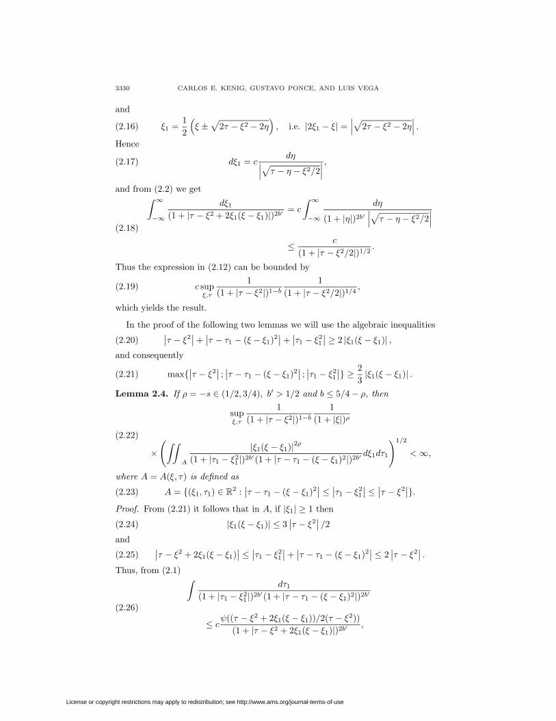
and
ξ1 =1
2
(ξ ±
√2τ − ξ2 − 2η
), i.e. |2ξ1 − ξ| =
∣∣∣√2τ − ξ2 − 2η∣∣∣ .(2.16)
Hence
dξ1 = cdη∣∣∣√τ − η − ξ2/2
∣∣∣ ,(2.17)
and from (2.2) we get∫ ∞−∞
dξ1(1 + |τ − ξ2 + 2ξ1(ξ − ξ1)|)2b′
= c
∫ ∞−∞
dη
(1 + |η|)2b′∣∣∣√τ − η − ξ2/2
∣∣∣≤ c
(1 + |τ − ξ2/2|)1/2.
(2.18)
Thus the expression in (2.12) can be bounded by
c supξ,τ
1
(1 + |τ − ξ2|)1−b1
(1 + |τ − ξ2/2|)1/4,(2.19)
which yields the result.
In the proof of the following two lemmas we will use the algebraic inequalities∣∣τ − ξ2∣∣+∣∣τ − τ1 − (ξ − ξ1)2
∣∣+∣∣τ1 − ξ2
1
∣∣ ≥ 2 |ξ1(ξ − ξ1)| ,(2.20)
and consequently
max{∣∣τ − ξ2
∣∣ ; ∣∣τ − τ1 − (ξ − ξ1)2∣∣ ; ∣∣τ1 − ξ2
1
∣∣} ≥ 2
3|ξ1(ξ − ξ1)| .(2.21)
Lemma 2.4. If ρ = −s ∈ (1/2, 3/4), b′ > 1/2 and b ≤ 5/4− ρ, then
supξ,τ
1
(1 + |τ − ξ2|)1−b1
(1 + |ξ|)ρ
×(∫∫
A
|ξ1(ξ − ξ1)|2ρ
(1 + |τ1 − ξ21 |)2b′(1 + |τ − τ1 − (ξ − ξ1)2|)2b′
dξ1dτ1
)1/2
<∞,
(2.22)
where A = A(ξ, τ) is defined as
A = {(ξ1, τ1) ∈ R2 :∣∣τ − τ1 − (ξ − ξ1)2
∣∣ ≤ ∣∣τ1 − ξ21
∣∣ ≤ ∣∣τ − ξ2∣∣}.(2.23)
Proof. From (2.21) it follows that in A, if |ξ1| ≥ 1 then
|ξ1(ξ − ξ1)| ≤ 3∣∣τ − ξ2
∣∣ /2(2.24)
and ∣∣τ − ξ2 + 2ξ1(ξ − ξ1)∣∣ ≤ ∣∣τ1 − ξ2
1
∣∣+∣∣τ − τ1 − (ξ − ξ1)2
∣∣ ≤ 2∣∣τ − ξ2
∣∣ .(2.25)
Thus, from (2.1) ∫dτ1
(1 + |τ1 − ξ21 |)2b′(1 + |τ − τ1 − (ξ − ξ1)2|)2b′
≤ cψ((τ − ξ2 + 2ξ1(ξ − ξ1))/2(τ − ξ2))
(1 + |τ − ξ2 + 2ξ1(ξ − ξ1)|)2b′,
(2.26)
License or copyright restrictions may apply to redistribution; see http://www.ams.org/journal-terms-of-use
QUADRATIC FORMS FOR THE 1-D SEMILINEAR SCHRODINGER EQUATION 3331
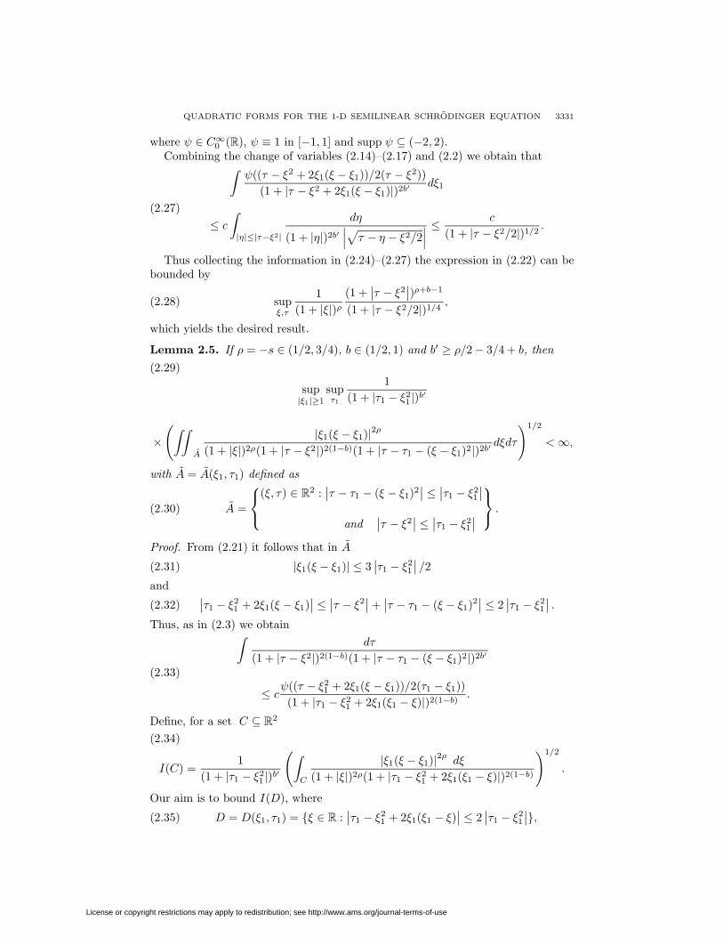
where ψ ∈ C∞0 (R), ψ ≡ 1 in [−1, 1] and supp ψ ⊆ (−2, 2).Combining the change of variables (2.14)–(2.17) and (2.2) we obtain that∫
ψ((τ − ξ2 + 2ξ1(ξ − ξ1))/2(τ − ξ2))
(1 + |τ − ξ2 + 2ξ1(ξ − ξ1)|)2b′dξ1
≤ c∫|η|≤|τ−ξ2|
dη
(1 + |η|)2b′∣∣∣√τ − η − ξ2/2
∣∣∣ ≤ c
(1 + |τ − ξ2/2|)1/2.
(2.27)
Thus collecting the information in (2.24)–(2.27) the expression in (2.22) can bebounded by
supξ,τ
1
(1 + |ξ|)ρ(1 +
∣∣τ − ξ2∣∣)ρ+b−1
(1 + |τ − ξ2/2|)1/4,(2.28)
which yields the desired result.
Lemma 2.5. If ρ = −s ∈ (1/2, 3/4), b ∈ (1/2, 1) and b′ ≥ ρ/2− 3/4 + b, then
sup|ξ1|≥1
supτ1
1
(1 + |τ1 − ξ21 |)b
′
×(∫∫
A
|ξ1(ξ − ξ1)|2ρ
(1 + |ξ|)2ρ(1 + |τ − ξ2|)2(1−b)(1 + |τ − τ1 − (ξ − ξ1)2|)2b′dξdτ
)1/2
<∞,
(2.29)
with A = A(ξ1, τ1) defined as
A =
(ξ, τ) ∈ R2 :
∣∣τ − τ1 − (ξ − ξ1)2∣∣ ≤ ∣∣τ1 − ξ2
1
∣∣and
∣∣τ − ξ2∣∣ ≤ ∣∣τ1 − ξ2
1
∣∣ .(2.30)
Proof. From (2.21) it follows that in A
|ξ1(ξ − ξ1)| ≤ 3∣∣τ1 − ξ2
1
∣∣ /2(2.31)
and ∣∣τ1 − ξ21 + 2ξ1(ξ − ξ1)
∣∣ ≤ ∣∣τ − ξ2∣∣+∣∣τ − τ1 − (ξ − ξ1)2
∣∣ ≤ 2∣∣τ1 − ξ2
1
∣∣ .(2.32)
Thus, as in (2.3) we obtain∫dτ
(1 + |τ − ξ2|)2(1−b)(1 + |τ − τ1 − (ξ − ξ1)2|)2b′
≤ cψ((τ − ξ21 + 2ξ1(ξ − ξ1))/2(τ1 − ξ1))
(1 + |τ1 − ξ21 + 2ξ1(ξ1 − ξ)|)2(1−b) .
(2.33)
Define, for a set C ⊆ R2
I(C) =1
(1 + |τ1 − ξ21 |)b
′
(∫C
|ξ1(ξ − ξ1)|2ρ dξ
(1 + |ξ|)2ρ(1 + |τ1 − ξ21 + 2ξ1(ξ1 − ξ)|)2(1−b)
)1/2
.
(2.34)
Our aim is to bound I(D), where
D = D(ξ1, τ1) = {ξ ∈ R :∣∣τ1 − ξ2
1 + 2ξ1(ξ1 − ξ)∣∣ ≤ 2
∣∣τ1 − ξ21
∣∣},(2.35)
License or copyright restrictions may apply to redistribution; see http://www.ams.org/journal-terms-of-use

3332 CARLOS E. KENIG, GUSTAVO PONCE, AND LUIS VEGA
uniformly in (ξ1, τ1) ∈ R2. We divide D into two subdomains D1 and D2. In
D1 = {ξ ∈ D : |2ξ1(ξ1 − ξ)| ≤∣∣τ1 − ξ2
1
∣∣ /2}(2.36)
one has that ∣∣τ1 − ξ21
∣∣ ≤ 2∣∣τ1 − ξ2
1 + 2ξ1(ξ1 − ξ)∣∣ ,(2.37)
and consequently
I(D1) ≤(1 +
∣∣τ1 − ξ21
∣∣)ρ(1 + |τ1 − ξ2
1 |)1−b+b′
(∫D1
dξ
(1 + |ξ|)2ρ
)1/2
< c.(2.38)
We subdivide D2, i.e.
D2 ={ξ ∈ D :
∣∣τ1 − ξ21
∣∣ /4 ≤ |ξ1(ξ1 − ξ)| ≤ 3∣∣τ1 − ξ2
1
∣∣ /2} ,(2.39)
into three pieces. First
D2,1 = {ξ ∈ D2 : |ξ|/4 ≤ |ξ1| ≤ 100|ξ|}.(2.40)
In this set
|ξ|2 ∼ |ξ1|2 ≥ c(1 +∣∣τ1 − ξ2
1
∣∣).(2.41)
Therefore using the change of variables
η = τ1 − ξ21 + 2ξ1(ξ1 − ξ), dη = −2ξ1dξ,(2.42)
we obtain
I(D2,1) ≤ c(1 +∣∣τ1 − ξ2
1
∣∣)ρ/2−b′ (∫|η|≤2|τ1−ξ2
1 |
1
|ξ1| (1 + |η|)2(1−b) dη
)1/2
≤ c(1 +∣∣τ1 − ξ2
1
∣∣)ρ/2−b′+3/4+b ≤ c.
(2.43)
In
D2,2 = {ξ ∈ D2 : 1 ≤ |ξ1| ≤ |ξ|/4}(2.44)
using (2.21) one has
I(D2,2) ≤ c(1 +∣∣τ1 − ξ2
1
∣∣)−b′ (∫|η|≤2|τ1−ξ2
1|
|ξ1|2ρ
|ξ1| (1 + |η|)2(1−b) dη
)1/2
≤ c(1 +∣∣τ1 − ξ2
1
∣∣)2ρ−1−b′+ρ−1/2+b−1/2.
(2.45)
Finally we consider
D2,3 = {ξ ∈ D2 : 100|ξ| ≤ |ξ1|}.(2.46)
In this region
|ξ1|2 ∼∣∣τ1 − ξ2
1
∣∣ .(2.47)
Hence,
I(D2,3) ≤ c(1 +∣∣τ1 − ξ2
1
∣∣)ρ−b′−3/4+b ≤ c,(2.48)
which completes the proof of (2.29).
License or copyright restrictions may apply to redistribution; see http://www.ams.org/journal-terms-of-use

QUADRATIC FORMS FOR THE 1-D SEMILINEAR SCHRODINGER EQUATION 3333
Proof of Theorem 2.2. First we consider the case s = 0. Combining Cauchy-Schwarz inequality, (2.12) and Fubini’s theorem, it follows that
∥∥∥∥ 1
(1 + |τ − ξ2|)1−b
∫∫f(ξ1, τ1)
(1 + |τ1 − ξ21 |)b
′g(ξ − ξ1, τ − τ1)
(1 + |τ − τ1 − (ξ − ξ1)2|)b′ dξ1dτ1∥∥∥∥L2L2
≤∥∥∥∥∥ 1
(1 + |τ − ξ2|)1−b
(∫∫dξ1dτ1
(1 + |τ − τ1 − (ξ − ξ1)2|)2b′
)1/2∥∥∥∥∥L∞ξ L
∞τ
×∥∥∥∥∥(∫∫
|f(ξ1, τ1)|2 |g(ξ − ξ1, τ − τ1)|2 dξ1dτ1)1/2
∥∥∥∥∥L2ξL
2τ
≤c‖f‖L2ξL
2τ‖g‖L2
ξL2τ
(2.49)
for any b′ > 1/2 and b ≤ 1. Taking b = b′ we obtain the result.Next we consider the case ρ = −s ∈ (1/2, 3/4). We observe that if
either |ξ1| ≤ 1 or |ξ − ξ1| ≤ 1,(2.50)
then
(1 + |ξ1|)ρ(1 + |ξ − ξ1|)ρ ≤ c(1 + |ξ|)ρ,(2.51)
which reduces the estimate to the previous case s = 0. Therefore, we assume
|ξ1| ≥ 1 and |ξ − ξ1| ≥ 1.(2.52)
Also by symmetry we can restrict ourselves to the case∣∣τ − τ1 − (ξ − ξ1)2∣∣ ≤ ∣∣τ1 − ξ2
1
∣∣ .(2.53)
Now we split the domain of integration into two pieces∣∣τ1 − ξ21
∣∣ ≤ ∣∣τ − ξ2∣∣ and
∣∣τ − ξ2∣∣ ≤ ∣∣τ1 − ξ2
1
∣∣ .(2.54)
In the first part, (∣∣τ1 − ξ2
1
∣∣ ≤ ∣∣τ − ξ2∣∣) we combine Cauchy-Schwarz and (2.22)
with b = b′, as in (2.49), to obtain the result. In the second part we use duality,Cauchy-Schwarz and (2.29) with b = b′ to complete the result.
Corollary 2.5. If ρ = −s ∈ (1/2, 3/4), b ∈ (1/2, 5/4 − ρ] and b′ > 1/2 withb− b′ ∈ (0, 3/4− ρ/2], then
‖B1(F, F )‖Xs,b−1≤ c‖F‖2Xs,b′ .(2.55)
Moreover (2.55) holds for s = 0, and 1/2 < b < b′ ≤ 1.
Proof of Theorem 1.4(i). For N ∈ Z+ define
fN(ξ, τ) = ψ(ξ −N)ψ(τ − ξ2)(2.56)
and
gN (ξ, τ) = ψ(ξ +N)ψ(τ − ξ2)(2.57)
where ψ ∈ C∞(R), ψ ≥ 0, ψ ≡ 1 in [−1, 1] and suppψ ⊆ [−2, 2]. A simplecomputation shows that for N large
(fN ∗ gN )(ξ, τ) ≥ c
Nψ(2N2 + τ/N)ψ(ξ).(2.58)
License or copyright restrictions may apply to redistribution; see http://www.ams.org/journal-terms-of-use

3334 CARLOS E. KENIG, GUSTAVO PONCE, AND LUIS VEGA
Thus (2.10) implies that
1
N2(1−b)N2ρ
N1/2≤ c.(2.59)
Now, taking
hN (ξ, τ) = ψ(ξ +N)ψ(τ + ξ2)(2.60)
we have that for N large
(fN ∗ hN )(ξ, τ) ∼= cχR(ξ, τ),(2.61)
where χA(·) denotes the characteristic function of the set A, and R is the rectangleof dimensions cN × N−1 centered in the origin with longest side pointing in the(1, 2N) direction.
Thus, (2.10) tells that
1
N1−bN2ρ
N2b≤ c.(2.62)
Combining (2.59), (2.62) and letting N tend to infinity, we obtain that
ρ ≤ min
{5
4− b; b
2+
1
2
},(2.63)
which completes the proof of Theorem 1.4(i).
Next, we deduce general estimates which are needed in the proof of Theorems1.5–1.7.
We denote by {eit∂2x}∞t=−∞ the unitary group describing the solution of the linear
IVP associated to (1.1). {∂tu− i∂2
xu = 0, t, x ∈ R,u(x, 0) = u0(x)
(2.64)
where
u(x, t) = eit∂2xu0(x) = c(e−itξ
2
u0(ξ))∨(x).(2.65)
We shall use the notations
‖f‖LpxLqt =
(∫ ∞−∞
(∫ ∞−∞|f(t, x)|q dt
)p/qdx
)1/p
,(2.66)
Jsh(ξ) = (1 + |ξ|)sh(ξ)(2.67)
and
Λbg(τ) = (1 + |τ |)bg(τ).(2.68)
The identity
‖F‖Xs,b =∥∥∥ΛbJseit∂
2xF∥∥∥L2xL
2t
(2.69)
describes the relationship between the spaces Xs,b’s and the group{eit∂
2x
}∞t=−∞
.
Let ψ ∈ C∞0 (R) with ψ ≡ 1 on [−1, 1] and suppψ ⊆ (−2, 2).
License or copyright restrictions may apply to redistribution; see http://www.ams.org/journal-terms-of-use
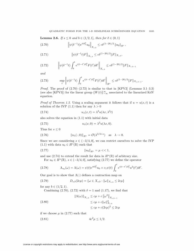
QUADRATIC FORMS FOR THE 1-D SEMILINEAR SCHRODINGER EQUATION 3335
Lemma 2.6. If s ≤ 0 and b ∈ (1/2, 1], then for δ ∈ (0, 1)∥∥∥ψ(δ−1t)eit∂2xu0
∥∥∥Xs,b≤ cδ(1−2b)/2 ‖u0‖Hs ,(2.70)
∥∥ψ(δ−1t)F∥∥Xs,b≤ cδ(1−2b)/2‖F‖Xs,b ,(2.71)
∥∥∥∥ψ(δ−1t)
∫ t
0
ei(t−t′)∂2
xF (t′)dt′∥∥∥∥Xs,b
≤ cδ(1−2b)/2‖F‖Xs,b−1(2.72)
and
supt
∥∥∥∥ψ(δ−1t)
∫ t
0
ei(t−t′)∂2
xF (t′)dt′∥∥∥∥Hs≤ cδ(1−2b)/2‖F‖Xs,b−1
.(2.73)
Proof. The proof of (2.70)–(2.72) is similar to that in [KPV2] (Lemmas 3.1–3.3)(see also [KPV3]) for the linear group {W (t)}∞−∞ associated to the linearized KdVequation.
Proof of Theorem 1.5. Using a scaling argument it follows that if u = u(x, t) is asolution of the IVP (1.1) then for any λ > 0
uλ(x, t) = λ2u(λx, λ2t)(2.74)
also solves the equation in (1.1) with initial data
uλ(x, 0) = λ2u(λx, 0).(2.75)
Thus for s ≤ 0
‖uλ(·, 0)‖Hs = O(λ3/2+s) as λ→ 0.(2.76)
Since we are considering s ∈ (−3/4, 0], we can restrict ourselves to solve the IVP(1.1) with data u0 ∈ Hs(R) such that
‖u0‖Hs = µ << 1,(2.77)
and use (2.74) to extend the result for data in Hs(R) of arbitrary size.For u0 ∈ Hs(R), s ∈ (−3/4, 0], satisfying (2.77) we define the operator
Λu0(ω) = Λ(ω) = ψ(t)eit∂2xu0 + c1ψ(t)
∫ t
0
ei(t−t′)∂2
xu2(t′)dt′.(2.78)
Our goal is to show that Λ(·) defines a contraction map on
Ds,b(2cµ) = {ω ∈ Xs,b : ‖ω‖Xs,b ≤ 2cµ}(2.79)
for any b ∈ (1/2, 1).Combining (2.70), (2.72) with δ = 1 and (1.17), we find that
‖Λ(ω)‖Xs,b ≤ cµ+ c∥∥ω2
∥∥Xs,b−1
≤ cµ+ c‖ω‖2Xs,b≤ cµ+ c(2cµ)2 ≤ 2cµ
(2.80)
if we choose µ in (2.77) such that
4c2µ ≤ 1/2.(2.81)
License or copyright restrictions may apply to redistribution; see http://www.ams.org/journal-terms-of-use

3336 CARLOS E. KENIG, GUSTAVO PONCE, AND LUIS VEGA
Similarly
‖Λ(ω)− Λ(ω)‖Xs,b ≤ c∥∥∥∥ψ(t)
∫ t
0
ei(t−t′)∂2
x(ω2 − ω2)dt′∥∥∥∥Xs,b
≤ c∥∥ω − ω2
∥∥Xs,b−1
= c ‖(ω + ω)(ω − ω)‖Xs,b−1
≤ 4c2µ ‖ω − ω‖Xs,b ≤1
2‖ω − ω‖Xs,b .
(2.82)
Thus, Λ(·) defines a contraction map, and consequently there exists a unique u ∈Ds,b(2cµ) such that
u(t) = ψ(t)
(eit∂
2xu0 + c1
∫ t
0
ei(t−t′)∂2
xu2(t′)dt′).(2.83)
Therefore in the time interval [−1, 1] solves the integral equation associated to theIVP (1.1) with N = N1(·) given by (1.7). Since u ∈ Xs,b, with b > 1/2, by theSobolev embedding theorem and (2.69) it follows that
u |[−1,1]∈ C([−1, 1] : Hs(R)).(2.84)
Finally we explain how to extend the uniqueness result in Ds,b(2cµ) to the wholespace Xs,b. First we restrict the time interval, i.e. consider Λu0(·) in (2.78) withψ(δ−1t), δ ∈ (0, 1), instead of ψ(t). Arguing as in [KPV2] we obtain estimatessimilar to those in (2.80), (2.82) but with a factor δθ0 , θ0 = θ0(b, b′) > 0, in theleft side, which allows us to establish the contraction principle in Ds,b(R) withR(δ)→∞ as δ → 0 (for details see [KPV2]).
3. Proof of Theorems 1.2, 1.4(ii) and 1.6
Define
ρ = −s ∈ [0, 1/4)(3.1)
and for F ∈ Xs,b = X−ρ,b
f(ξ, τ) = (1 +∣∣τ − ξ2
∣∣)b(1 + |ξ|)−ρF (ξ, τ) ∈ L2(R2),(3.2)
thus
‖f‖L2ξL
2τ
= ‖F‖Xs,b .(3.3)
Since
¯F (ξ, τ) = ˆF (−ξ,−τ)(3.4)
it follows that
ˆF (ξ, τ) =(1 + |ξ|)ρ
(1 + |τ + ξ2|)b f(−ξ,−τ)(3.5)
with
‖f‖L2ξL
2τ
= ‖F‖Xs,b .(3.6)
License or copyright restrictions may apply to redistribution; see http://www.ams.org/journal-terms-of-use

QUADRATIC FORMS FOR THE 1-D SEMILINEAR SCHRODINGER EQUATION 3337
Thus we can rewrite (1.18) in terms of f as
‖B2(F, F )‖Xs,b−1=∥∥∥(1 +
∣∣τ − ξ2∣∣)b−1(1 + |ξ|)−ρF F
∥∥∥L2ξL
2τ
=∥∥∥(1 +
∣∣τ − ξ2∣∣)b−1(1 + |ξ|)−ρ(F ∗ ˆF )
∥∥∥L2ξL
2τ
=c
∥∥∥∥ 1
(1 + |τ − ξ2|)1−b(1 + |ξ|)ρ
×∫∫
f(ξ − ξ1, τ − τ1)(1 + |ξ − ξ1|)ρ(1 + |τ − τ1 − (ξ − ξ1)2|)b
f(−ξ1,−τ1)(1 + |ξ1|)ρ(1 + |τ1 + ξ2
1 |)bdξ1dτ1
∥∥∥∥L2ξL
2τ
.
(3.7)
Defining
B2(f, g, ρ, b)(ξ, τ) =1
(1 + |τ − ξ2|)1−b(1 + |ξ|)ρ
×∫∫
f(ξ1, τ1)(1 + |ξ1|)ρ(1 + |τ1 + ξ2
1 |)bg(ξ − ξ1, τ − τ1)(1 + |ξ − ξ1|)ρ
(1 + |τ − τ1 − (ξ − ξ1)2|)b dξ1dτ1,
(3.8)
Theorem 1.2 can be rewritten as follows.
Theorem 3.1. Given ρ = −s ∈ [0, 1/4) there exists b ∈ (1/2, 1) such that
‖B2(f, g, ρ, b)‖L2ξL
2τ≤ c‖f‖L2
ξL2τ‖g‖L2
ξL2τ.(3.9)
The proof of Theorem 3.1 will be deduced from the following lemmas.
Lemma 3.2. If b ∈ (1/2, 1], then
‖B2(f, g, 0, b)‖L2ξL
2τ≤ c‖f‖L2
ξL2τ‖g‖L2
ξL2τ.(3.10)
Proof. It will be shown that
sup|ξ|≥1
supτ
1
(1 + |τ − ξ2|)1−b
×(∫∫
dτ1dξ1(1 + |τ1 + ξ2
1 |)2b(1 + |τ − τ1 − (ξ − ξ1)2|)2b
)1/2
<∞
(3.11)
and
supξ1,τ1
1
(1 + |τ1 + ξ21 |)b
×(∫|ξ|≤1
∫dτdξ
(1 + |τ − ξ2|)2(1−b)(1 + |τ − τ1 − (ξ − ξ1)2|)2b
)1/2
<∞.
(3.12)
It is easy to see that (3.10) follows by combining (3.11)–(3.12), Cauchy-Schwarzand duality.
To prove (3.11) we first use (2.1) to find that∫dτ1
(1 + |τ1 + ξ21 |)2b(1 + |τ − τ1 − (ξ − ξ1)2|)2b
≤ c
(1 + |τ − ξ2 + 2ξξ1|)2b.(3.13)
License or copyright restrictions may apply to redistribution; see http://www.ams.org/journal-terms-of-use

3338 CARLOS E. KENIG, GUSTAVO PONCE, AND LUIS VEGA
Next, changing variables
η1 = τ − ξ2 + 2ξξ1, dη1 = 2ξdξ1,(3.14)
it follows that ∫dξ1
(1 + |τ − ξ2 + 2ξξ1|)2b≤ c
∫dη1
|ξ|(1 + |η1|)2b≤ c′
|ξ| .(3.15)
Inserting (3.15) in (3.13) we obtain (3.11). To prove (3.12) we use (2.3) to concludethat ∫
|ξ|≤1
(∫dτ
(1 + |τ − ξ2|)2(1−b)(1 + |τ − τ1 − (ξ − ξ1)2|)2b
)dξ
≤ c∫|ξ|≤1
dξ
(1 + |τ1 + ξ21 − 2ξξ1|)2(1−b) ≤ 2c,
(3.16)
which yields (3.12).
In the next proofs we will use the following algebraic relations∣∣τ − τ1 − (ξ − ξ1)2∣∣+∣∣τ1 + ξ2
1
∣∣+∣∣τ − ξ2
∣∣ ≥ 2 |ξξ1|(3.17)
and consequently
max{∣∣τ − τ1 − (ξ − ξ1)2
∣∣ ; ∣∣τ1 + ξ21
∣∣ ; ∣∣τ − ξ2∣∣} ≥ 2 |ξξ1| /3.(3.18)
Lemma 3.3. If ρ = −s ∈ [0, 1/4), then there exists b > 1/2 such that
sup|ξ|≥1
supτ
1
(1 + |τ − ξ2|)1−b1
(1 + |ξ|)ρ
×(∫∫
A1
|ξ1(ξ − ξ1)|2ρ
(1 + |τ1 + ξ21 |)2b(1 + |τ − τ1 − (ξ − ξ1)2|)2b
dξ1dτ1
)1/2
<∞
(3.19)
where A1 = A1(ξ, τ) is defined as
A1 =
(ξ1, τ1) ∈ R2 : |ξ1| ≥ 10, |ξ − ξ1| ≥ 10∣∣τ − τ1 − (ξ − ξ1)2
∣∣ ≤ ∣∣τ − ξ2∣∣
and∣∣τ1 + ξ2
1
∣∣ ≤ ∣∣τ − ξ2∣∣
.(3.20)
Proof. From (2.1) it follows that∫τ1∈A1
dτ1(1 + |τ1 + ξ2
1 |)2b(1 + |τ − τ1 − (ξ − ξ1)2|)2b
≤ψ((τ − ξ2 + 2ξξ1)/2(τ − ξ2))
(1 + |τ − ξ2 + 2ξξ1|)2b,
(3.21)
and changing variable as in (3.14)
∫|τ−ξ2+2ξξ1|≤2|τ−ξ2|
dξ1(1 + |τ − ξ2 + 2ξξ1|)2b
≤ c 1
|ξ|
∫|η1|≤2|τ−ξ2|
dη1
(1 + |η1|)2b≤ c
(3.22)
since |ξ| ≥ 1.
License or copyright restrictions may apply to redistribution; see http://www.ams.org/journal-terms-of-use

QUADRATIC FORMS FOR THE 1-D SEMILINEAR SCHRODINGER EQUATION 3339
In A1, (3.18) and the hypothesis guarantee that there exists b > 1/2 such that
|ξ1(ξ − ξ1)|2ρ ≤ c∣∣τ − ξ2
∣∣4ρ ≤ c ∣∣τ − ξ2∣∣2(1−b)
,(3.23)
thus by inserting (3.21)–(3.23) in (3.19) we obtain the desired result.
Lemma 3.4. If ρ = −s ∈ [0, 1/4), then there exists b > 1/2 such that
sup|ξ1|≥10
supτ1
1
(1 + |τ1 + ξ21 |)b
×(∫∫
|ξ|≤1
|ξ1(ξ − ξ1)|2ρ dξdτ(1 + |ξ|)2ρ(1 + |τ − τ1 − (ξ − ξ1)2|)2b(1 + |τ − ξ2|)2(1−b)
)1/2
<∞.
(3.24)
Proof. Using (2.3) we find that
∫dτ
(1 + |τ − τ1 − (ξ − ξ1)2|)2b(1 + |τ − ξ2|)2(1−b) ≤c
(1 + |τ1 + ξ21 − 2ξξ1|)2(1−b) ,
(3.25)
and by changing variables
η = τ1 + ξ21 − 2ξξ1, dη = −2ξ1dξ,(3.26)
we get (∫|ξ|≤1
|ξ1(ξ − ξ1)|2ρ
(1 + |τ1 + ξ21 − 2ξξ1|2(1−b) dξ
)1/2
≤c |ξ1|2ρ
|ξ1|1/2
(∫|η|≤|τ1+ξ2
1 |+2|ξ1|
dη
(1 + |η|)2(1−b)
)1/2
≤c |ξ1|2ρ−1/2(
(1 +∣∣τ1 + ξ2
1
∣∣)b−1/2 + |ξ1|b−1/2).
(3.27)
Thus we obtain the following bound for the term in (3.24)
sup|ξ1|≥10
supτ1
|ξ1|2ρ−1/2
(1 + |τ1 + ξ21 |)b
((1 +
∣∣τ1 + ξ21
∣∣)b−1/2 + |ξ1|b−1/2),(3.28)
which yields the result.
Lemma 3.5. If ρ = −s ∈ [0, 1/4), then there exists b > 1/2 such that
sup|ξ1|≥10
supτ1
1
(1 + |τ1 + ξ21 |)b
×(∫∫
B1
|ξ1(ξ − ξ1)|2ρ dξdτ(1 + |ξ|)2ρ(1 + |τ − τ1 − (ξ − ξ1)2|)2b(1 + |τ − ξ2|)2(1−b)
)1/2
<∞
(3.29)
License or copyright restrictions may apply to redistribution; see http://www.ams.org/journal-terms-of-use

3340 CARLOS E. KENIG, GUSTAVO PONCE, AND LUIS VEGA
where B1 = B1(ξ1, τ1) is defined as
B1 =
(ξ, τ) ∈ R2 :
∣∣τ − τ1 − (ξ − ξ1)2∣∣ ≤ ∣∣τ1 + ξ2
1
∣∣∣∣τ − ξ2
∣∣ ≤ ∣∣τ1 + ξ21
∣∣|ξ − ξ1| ≥ 10 and |ξ| ≥ 1
.(3.30)
Proof. Arguing as in the previous proof, using that in B1
|η| =∣∣τ1 + ξ2
1 − 2ξξ1∣∣ ≤ 2
∣∣τ1 + ξ21
∣∣(3.31)
and also using (3.17), we see that the expression in (3.29) can be bounded by
sup|ξ1|≥10
supτ
(1 +∣∣τ1 + ξ2
1
∣∣)2ρ−1/2,(3.32)
which yields the result.
Lemma 3.6. If ρ = −s ∈ [0, 1/4), then there exists b > 1/2 such that
sup|ξ1|≥10
supτ1
1
(1 + |τ1 − ξ21 |)b
×(∫∫
C
|ξ1(ξ − ξ1)|2ρ dτdξ(1 + |ξ|)2ρ(1 + |τ − τ1 + (ξ − ξ1)2|)2b(1 + |τ − ξ2|)2(1−b)
)1/2
<∞
(3.33)
where C = C(ξ1, τ1) is defined as
C =
(ξ, τ) ∈ R2 :
∣∣τ − τ1 + (ξ − ξ1)2∣∣ ≤ ∣∣τ1 − ξ2
1
∣∣∣∣τ − ξ2
∣∣ ≤ ∣∣τ1 − ξ21
∣∣|ξ| ≥ 1 and |ξ − ξ1| ≥ 10
.(3.34)
Proof. From (2.3) it follows that∫τ∈C
dτ
(1 + |τ − τ1 + (ξ − ξ1)2|)2b(1 + |τ − ξ2|)2(1−b)
≤cψ((τ1 − ξ2
1 − 2ξ(ξ − ξ1))/2(τ1 − ξ21))
(1 + |τ1 − ξ21 − 2ξ(ξ − ξ1)|)2(1−b)
(3.35)
since in C∣∣τ1 − ξ21 − 2ξ(ξ − ξ1)
∣∣ ≤ ∣∣τ − τ1 + (ξ − ξ1)2∣∣+∣∣τ − ξ2
∣∣ ≤ 2∣∣τ1 − ξ2
1
∣∣ .(3.36)
Also we observe that in C (see (3.17))∣∣τ1 − ξ21
∣∣ ≥ c |ξξ1| .(3.37)
Next we introduce the notation
I(E) =1
(1 + |τ1 − ξ21 |)b
(∫E
|ξ1(ξ − ξ1)|2ρ
(1 + |ξ|)2ρ(1 + |τ1 − ξ21 − 2ξ(ξ − ξ1)|)2(1−b) dξ
)1/2
.
(3.38)
License or copyright restrictions may apply to redistribution; see http://www.ams.org/journal-terms-of-use

QUADRATIC FORMS FOR THE 1-D SEMILINEAR SCHRODINGER EQUATION 3341
Our aim is to bound I(D) where
D =
ξ ∈ C :
∣∣τ1 − ξ21 − 2ξ(ξ − ξ1)
∣∣ ≤ 2∣∣τ1 − ξ2
1
∣∣|ξ| ≥ 1 and |ξ − ξ1| ≥ 10
.(3.39)
Changing variables
η = τ1 − ξ21 − 2ξ(ξ − ξ1), dη = 2(ξ1 − 2ξ)dξ = 2
√2τ1 − 2η − ξ2
1dξ(3.40)
and splitting D into three parts, D1, D2, D3 we have, in D1, i.e.
D1 = {ξ ∈ D : |ξ1| ≤ 100|ξ|}(3.41)
from (3.37), (2.4) it follows that
I(D1) ≤ 1
(1 + |τ1 − ξ21 |)b−ρ
(∫|η|≤2|τ1−ξ2
1|
dη
(1 + |η|)2(1−b)√|2τ1 − 2η − ξ2
1 |
)1/2
≤ c(1 +
∣∣τ1 − ξ21
∣∣)ρ−1/4
(1 + |2τ1 − ξ21 |)1/4
< c′.
(3.42)
In D2, i.e.
D2 = {ξ ∈ D : |ξ1| ≥ 100|ξ| and |ξ1| ≤ 500∣∣τ1 − ξ2
1
∣∣}(3.43)
we have that the change of variable (3.40) satisfies
|ξ1 − 2ξ| ∼ |ξ1| and dη ' ξ1dξ.(3.44)
Therefore
I(D2) ≤ c |ξ1|2ρ−1/2
(1 + |τ1 − ξ21 |)b
(∫|η|≤2|τ1−ξ2
1|
dη
(1 + |η|)2(1−b)
)1/2
≤ c(1 +
∣∣τ1 − ξ21
∣∣)2ρ−1/2
(1 + |τ1 − ξ21 |)b
(1 +∣∣τ1 − ξ2
1
∣∣)b−1/2 ≤ c′.
(3.45)
Finally, a simple computation shows that
D3 = {ξ ∈ D : |ξ1| ≥ 100|ξ| ,∣∣τ1 − ξ2
1
∣∣ ≤ |ξ1| /500}(3.46)
is empty.
Proof of Theorem 1.4(ii). For N ∈ Z+ we define
fN(ξ, τ) = ψ(ξ −N)ψ(τ − ξ2)(3.47)
and
pN(ξ, τ) = ψ(ξ +N)ψ(τ + ξ2).(3.48)
Thus
(fN ∗ pN )(ξ, τ) ∼ cχR0(ξ, τ)(3.49)
where χA(·) denotes the characteristic function of the set A, and R0 is the rectangleof dimensions N × N−1 centered at the origin with longest side pointing in the(1, 2N) direction.
License or copyright restrictions may apply to redistribution; see http://www.ams.org/journal-terms-of-use

3342 CARLOS E. KENIG, GUSTAVO PONCE, AND LUIS VEGA
Finally from (3.9) it follows that for N large
N2s ≥ c(∫|ξ|≤1
∫|τ |<1
χR0(ξ, τ)dξdτ
)1/2
≥ cN−1/2.(3.50)
Once Theorem 1.2 is available the proof of Theorem 1.6 reduces to that given insection 2 for Theorem 1.5, therefore it will be omitted.
4. Proof of Theorems 1.3, 1.4(iii) and 1.7
Define
ρ = −s ∈ [0, 3/4)(4.1)
and
f(ξ, τ) = (1 +∣∣τ − ξ2
∣∣)b(1 + |ξ|)−ρF (ξ, τ) ∈ L2(R2).(4.2)
The argument in section 2 shows that
‖f‖L2ξL
2τ
= ‖F‖Xs,b .(4.3)
Thus B3 can be expressed in terms of f as
‖B3(F, F )‖Xs,b−1=∥∥∥(1 +
∣∣τ − ξ2∣∣)b−1(1 + |ξ|)−ρFF∥∥∥
L2ξL
2τ
=∥∥∥(1 +
∣∣τ − ξ2∣∣)b−1(1 + |ξ|)−ρ( F ∗ F )
∥∥∥L2ξL
2τ
= c
∥∥∥∥ 1
(1 + |τ − ξ2|)1−b(1 + |ξ|)ρ×∫∫f(ξ1 − ξ, τ1 − τ)(1 + |ξ − ξ1|)ρ
(1 + |τ − τ1 + (ξ − ξ1)2|)bf(−ξ1,−τ1)(1 + |ξ1|)ρ
(1 + |τ1 + ξ21 |)b
dξ1dτ1
∥∥∥∥L2ξL
2τ
.
(4.4)
Defining
B3(f, g, ρ, b)(ξ, τ) =1
(1 + |τ − ξ2|)1−b(1 + |ξ|)ρ ×∫∫f(ξ1, τ1)(1 + |ξ1|)ρ
(1 + |τ1 + ξ21 |)b
g(ξ − ξ1, τ − τ1)(1 + |ξ − ξ1)|)ρ(1 + |τ − τ1 + (ξ − ξ1)2|)b dξ1dτ1,
(4.5)
Theorem 1.2 can be rewritten as follows.
Theorem 4.1. Given ρ = −s ∈ [0, 3/4) there exists b ∈ (1/2, 1) such that
‖B3(f, g, ρ, b)‖L2ξL
2τ≤ c‖f‖L2
ξL2τ‖g‖L2
ξL2τ.(4.6)
The proof of Theorem 4.1 will be a direct consequence of the following lemmas.
Lemma 4.2. If b ∈ (1/2, 1], then
‖B3(f, g, 0, b)‖L2ξL
2τ≤ c‖f‖L2
ξL2τ‖g‖L2
ξL2τ.(4.7)
License or copyright restrictions may apply to redistribution; see http://www.ams.org/journal-terms-of-use

QUADRATIC FORMS FOR THE 1-D SEMILINEAR SCHRODINGER EQUATION 3343
Proof. It suffices to see that
supξ,τ
1
(1 + |τ − ξ2|)1−b
(∫∫dξ1dτ1
(1 + |τ1 + ξ21 |)2b(1 + |τ − τ1 + (ξ − ξ1)2|)2b
)1/2
<∞.
(4.8)
By changing variables (ξ, ξ1, τ, τ1) → −(ξ, ξ1, τ, τ1), the integral in (4.8) is thesame as that in (2.12) (Lemma 2.3). Following its proof we obtain the bound
supξ,τ
1
(1 + |τ + ξ2|)1−b1
(1 + |τ − ξ2/2|)1/4,(4.9)
which yields the result.
In the proof of the following lemmas we use the algebraic relations
τ − τ1 + (ξ − ξ1)2 + τ1 + ξ21 − (τ − ξ2) = (ξ − ξ1)2 + ξ2
1 + ξ2,(4.10)
and consequently
max{∣∣τ − ξ2
∣∣ ; ∣∣τ1 + ξ21
∣∣ ; ∣∣τ − τ1 + (ξ − ξ1)2∣∣} ≥ 1
3(ξ2
1 + ξ2 + (ξ − ξ1)2).(4.11)
Lemma 4.3. If ρ = −s ∈ (1/2, 3/4) and b ∈ (1/2, 5/4− s), then
supξ,τ
1
(1 + |τ − ξ2|)1−b1
(1 + |ξ|)ρ
×(∫∫
A3
|ξ1(ξ − ξ1)|2ρ
(1 + |τ1 + ξ21 |)2b(1 + |τ − τ1 + (ξ − ξ1)2|)2b
dτ1dξ1
)1/2
<∞
(4.12)
where A3 = A3(ξ, τ) is defined as
A3 = {(ξ1, τ1) :∣∣τ − τ1 + (ξ − ξ1)2
∣∣ ≤ ∣∣τ1 + ξ21
∣∣ ≤ ∣∣τ − ξ2∣∣}.(4.13)
Proof. Changing (τ, τ1) by −(τ, τ1) and following the argument in the proof ofLemma 2.4 (2.22) one obtains the following bound for (4.12)
supξ,τ
1
(1 + |ξ|)ρ(1 +
∣∣τ + ξ2∣∣)ρ+b−1
(1 + |τ − ξ2/2|)1/4,(4.14)
which yields the result.
Lemma 4.4. If ρ = −s ∈ (1/2, 3/4], then there exists b > 1/2 such that
sup|ξ1|≥1
supτ1
1
(1 + |τ1 + ξ21 |)b
×(∫∫
B3
|ξ1(ξ − ξ1)|2ρ
(1 + |ξ|)ρ(1 + |τ − ξ2|)2(1−b)(1 + |τ − τ1 + (ξ − ξ1)2|)2bdτdξ
)1/2
<∞
(4.15)
where B3 = B3(ξ1, τ1) is defined as
B3 =
(ξ, τ) ∈ R2 :
∣∣τ − τ1 + (ξ − ξ1)2∣∣ ≤ ∣∣τ1 + ξ2
1
∣∣and
∣∣τ − ξ2∣∣ ≤ ∣∣τ1 + ξ2
1
∣∣ .(4.16)
License or copyright restrictions may apply to redistribution; see http://www.ams.org/journal-terms-of-use

3344 CARLOS E. KENIG, GUSTAVO PONCE, AND LUIS VEGA
Proof. Following an argument similar to that used in the proof of Lemma 2.5, webound (4.15) by
sup|ξ1|≥1,τ1
1
(1 + |τ1 + ξ21 |)b
(∫D′
|ξ1(ξ − ξ1)|2ρ dξ
(1 + |ξ|)2ρ(1 + |τ1 − ξ2 − (ξ − ξ1)2|)2(1−b)
)1/2
(4.17)
with D′ = D′(ξ),
D′ = {ξ ∈ R :∣∣τ1 − ξ2 − (ξ − ξ1)2
∣∣ ≤ 2∣∣τ1 + ξ2
1
∣∣}.(4.18)
First we consider the subset of D′
D′1 = {ξ ∈ D′ : ξ2 + (ξ − ξ1)2 + ξ21 ≤
∣∣τ1 + ξ21
∣∣ /2}.(4.19)
In this domain it follows that
1
(1 + |τ1 + ξ21 |)b
(∫D′1
|ξ1(ξ − ξ1)|2ρ
(1 + |ξ|)2ρ(1 + |τ1 − ξ2 − (ξ − ξ1)2|)2(1−b) dξ
)1/2
≤(1 +
∣∣τ1 + ξ21
∣∣)ρ(1 + |τ1 + ξ2
1 |)
(∫dξ
(1 + |ξ|)2ρ
)1/2
<∞.(4.20)
Next we consider the remaining part of D1, i.e.
D′2 = {ξ ∈ D′ :∣∣τ1 + ξ2
1
∣∣ /2 ≤ ξ2 + (ξ − ξ1)2 + ξ21 ≤ 3
∣∣τ1 + ξ21
∣∣}.(4.21)
We split D′2 into three pieces D′2,1, D′2,2 and D′2,3. In D′2,1, i.e.
D′2,1 = {ξ ∈ D′2 : |ξ|/4 ≤ |ξ1| ≤ 100|ξ|},(4.22)
combining the change of variables
η = τ1 − ξ2 − (ξ − ξ1)2, dη = −2(ξ1 − 2ξ)dξ, |ξ1 − 2ξ| '√
(2τ1 − ξ2)/2− η),
(4.23)
so that since |ξ| ' |ξ1| we write
1
(1 + |τ1 + ξ21 |)b
(∫D′2,1
|ξ1(ξ − ξ1)|2ρ
(1 + |ξ|)2ρ(1 + |τ1 − ξ2 − (ξ − ξ1)2|)2(1−b) dξ
)1/2
≤c(1 +
∣∣τ1 + ξ21
∣∣)ρ/2(1 + |τ1 + ξ2
1 |)b
( ∫|η|≤3|τ1+ξ2
1|dη√
(2τ1 − ξ2)/2− η)(1 + |η|)2(1−b)
)1/2
≤c (1 + |τ1 + ξ21 |)ρ/2−1/4
(1 + |2τ1 − ξ21 |)1/4
≤ c.
(4.24)
In D′2,2, i.e.
D′2,2 = {ξ ∈ D′2 : 1 ≤ |ξ1| ≤ |ξ|/4},(4.25)
one has in (4.23) that |ξ1| /|ξ| < 1, hence, the argument in (4.24) extends to thiscase.
Finally we consider
D′2,3 = {ξ ∈ D′1 : 100|ξ| ≤ |ξ1|}.(4.26)
License or copyright restrictions may apply to redistribution; see http://www.ams.org/journal-terms-of-use
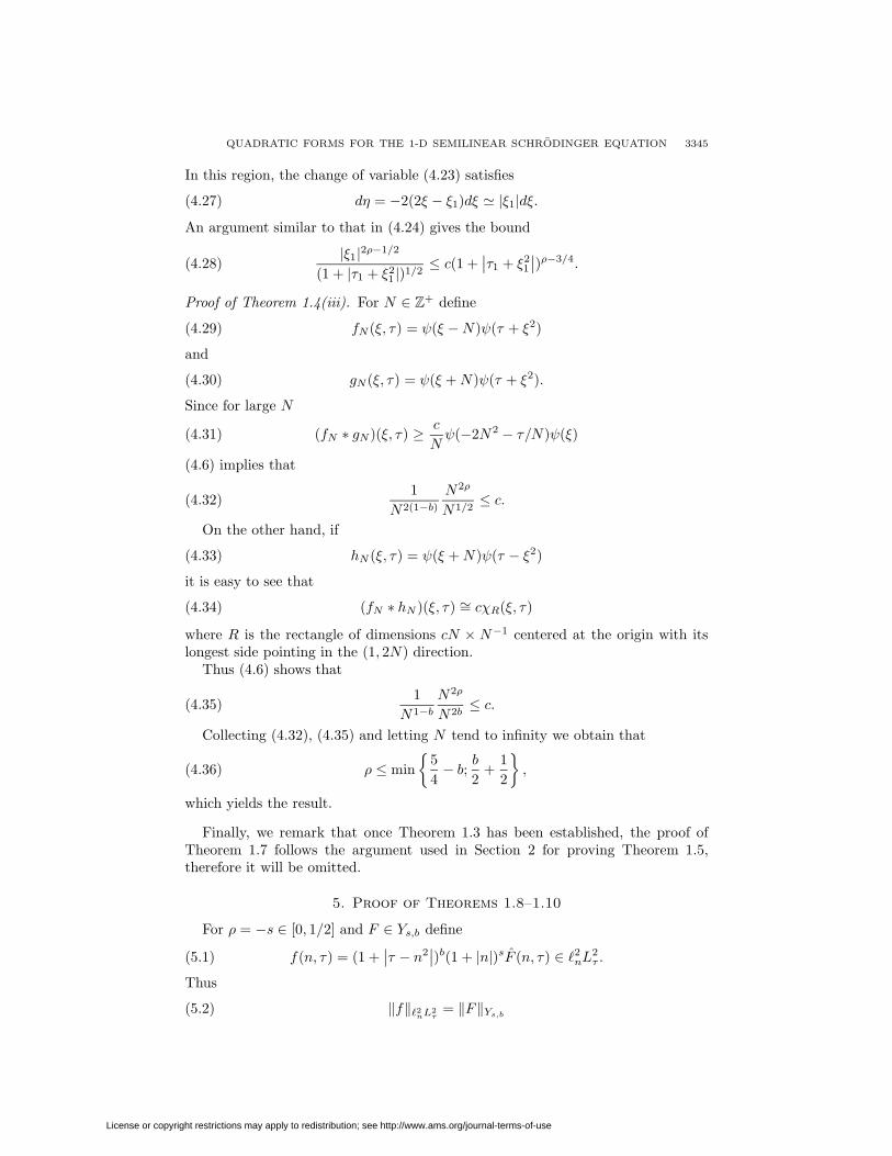
QUADRATIC FORMS FOR THE 1-D SEMILINEAR SCHRODINGER EQUATION 3345
In this region, the change of variable (4.23) satisfies
dη = −2(2ξ − ξ1)dξ ' |ξ1|dξ.(4.27)
An argument similar to that in (4.24) gives the bound
|ξ1|2ρ−1/2
(1 + |τ1 + ξ21 |)1/2
≤ c(1 +∣∣τ1 + ξ2
1
∣∣)ρ−3/4.(4.28)
Proof of Theorem 1.4(iii). For N ∈ Z+ define
fN(ξ, τ) = ψ(ξ −N)ψ(τ + ξ2)(4.29)
and
gN(ξ, τ) = ψ(ξ +N)ψ(τ + ξ2).(4.30)
Since for large N
(fN ∗ gN)(ξ, τ) ≥ c
Nψ(−2N2 − τ/N)ψ(ξ)(4.31)
(4.6) implies that
1
N2(1−b)N2ρ
N1/2≤ c.(4.32)
On the other hand, if
hN (ξ, τ) = ψ(ξ +N)ψ(τ − ξ2)(4.33)
it is easy to see that
(fN ∗ hN )(ξ, τ) ∼= cχR(ξ, τ)(4.34)
where R is the rectangle of dimensions cN × N−1 centered at the origin with itslongest side pointing in the (1, 2N) direction.
Thus (4.6) shows that
1
N1−bN2ρ
N2b≤ c.(4.35)
Collecting (4.32), (4.35) and letting N tend to infinity we obtain that
ρ ≤ min
{5
4− b; b
2+
1
2
},(4.36)
which yields the result.
Finally, we remark that once Theorem 1.3 has been established, the proof ofTheorem 1.7 follows the argument used in Section 2 for proving Theorem 1.5,therefore it will be omitted.
5. Proof of Theorems 1.8–1.10
For ρ = −s ∈ [0, 1/2] and F ∈ Ys,b define
f(n, τ) = (1 +∣∣τ − n2
∣∣)b(1 + |n|)sF (n, τ) ∈ `2nL2τ .(5.1)
Thus
‖f‖`2nL2τ
= ‖F‖Ys,b(5.2)
License or copyright restrictions may apply to redistribution; see http://www.ams.org/journal-terms-of-use

3346 CARLOS E. KENIG, GUSTAVO PONCE, AND LUIS VEGA
and (1.27) can be rewritten in terms of f
‖B1(F, F )‖Ys,b−1=∥∥∥(1 +
∣∣τ − n2∣∣)b−1(1 + |n|)sF 2
∥∥∥`2nL
2τ
=∥∥∥(1 +
∣∣τ − n2∣∣)b−1(1 + |n|)s(F ∗ F )
∥∥∥`2nL
2τ
=
∥∥∥∥ 1
(1 + |τ − n2|)1−b(1 + |n|)ρ
×∑n1
∫f(n1, τ1)(1 + |n1|)ρ
(1 + |τ1 − n21|)b
f(n− n1, τ − τ1)(1 + |n− n1|)ρ(1 + |τ − τ1 − (n− n1)2|)b dτ1
∥∥∥∥`2nL
2τ
.
(5.3)
Defining
B1(f, g, ρ, b, b′)(n, τ) =1
(1 + |τ − n2|)1−b(1 + |n|)ρ
×∑n1
∫f(n1, τ1)(1 + |n1|)ρ
(1 + |τ1 − n21|)b
′g(n− n1, τ − τ1)(1 + |n− n1|)ρ
(1 + |τ − τ1 − (n− n1)2|)b′ dτ1
(5.4)
we restate Theorem 1.8.
Theorem 5.1. If ρ = −s ∈ [0, 1/2], then
‖B1(f, g, ρ, 1/2, 1/2)‖`2nL2τ≤ c‖f‖`2nL2
τ‖g‖`2nL2
τ.(5.5)
As a consequence of the proof of Theorem 5.1 we have
Corollary 5.2. If ρ = −s ∈ [0, 1/2) and 1− b, b′ ≥ ρ with 1− b, b′ > 3/8, then
‖B1(f, g, ρ, b, b′)‖`2nL2τ≤ c‖f‖`2nL2
τ‖g‖`2nL2
τ.(5.6)
The following lemmas will be needed in the proof of Theorems 1.8–1.9.
Lemma 5.3. If γ > 1/2, then
sup(n,τ)∈Z×R
∞∑n1=−∞
1
(1 + |τ ± n1(n− n1)|)γ <∞.(5.7)
Proof. We rewrite (5.7)
∞∑n1=−∞
1
(1 + |τ ± n1(n− n1)|)γ =∑n1
1
(1 + |(n1 − α±)(n1 − β±)|)γ(5.8)
where α = α±(n, τ), β = β±(n, τ) are the roots of the polynomial
τ ± (n1(n− n1) = 0, i.e. τ ± n1(n− n1) = (n1 − α±)(n1 − β±).(5.9)
There are at most 10 n′1’s such that |n1 − α| ≤ 2 or |n1 − β| ≤ 2. The remainingn1’s satisfy
(1 + |(n1 − α)(n1 − β)|) ≥ 1
2(1 + |n1 − α|)(1 + |n1 − β|).(5.10)
Hence, applying the Cauchy-Schwarz inequality in (5.7) we obtain the desired result.
License or copyright restrictions may apply to redistribution; see http://www.ams.org/journal-terms-of-use

QUADRATIC FORMS FOR THE 1-D SEMILINEAR SCHRODINGER EQUATION 3347
In the proof of the following lemmas the following algebraic relation will be used
τ − n2 − (τ1 − n21)− (τ − τ1 − (n− n1)2) = −2n1(n− n1).(5.11)
In particular, this guarantees that
max{∣∣τ − n2
∣∣ ; ∣∣τ1 − n21
∣∣ ; ∣∣τ − τ1 − (n− n1)2∣∣} ≥ 2
3|n1(n− n1)| .(5.12)
Lemma 5.4. If ρ = −s ∈ [0, 1/2], then
sup(n,τ)∈Z×R
1
(1 + |τ − n2|)1/2
1
(1 + |n|)ρ
×(∑n1∈A
∫τ1∈A
(1 + |n1|)2ρ(1 + |n− n1|)2ρ
(1 + |τ1 − n21|)(1 + |τ − τ1 − (n− n1)2|)
)1/2
<∞
(5.13)
where A = A(n, τ) is defined as
A = {(n1, τ1) ∈ Z× R :∣∣τ − τ1 − (n− n1)2
∣∣ ≤ |τ1 − n1| ≤∣∣τ − n2
∣∣}.(5.14)
Proof. It suffices to consider the extremal cases, ρ = 0 and ρ = 1/2. If ρ = 0,changing variables
θ1 = τ1 − n21(5.15)
it follows that ∫τ1∈A
dτ1(1 + |τ1 − n2
1|)(1 + |τ − τ1 − (n− n1)2|)
=
∫dθ1
(1 + |θ1|)(1 + |θ1 − (τ − n2 + 2n1(n− n1))|)
≤`n(2 +
∣∣τ − n2 + 2n1(n− n1)∣∣)
(1 + |τ − n2 + 2n1(n− n1)|) .
(5.16)
Thus we have bound the term in (5.13) by
sup(n,τ)∈Z×R
(∑n1
`n(2 +∣∣τ − n2 + 2n1(n− n1)
∣∣)1 + |τ − n2 + 2n1(n− n1)|
)1/2
.(5.17)
Hence (5.7) completes the proof.
We observe that the factor(1 +
∣∣τ − n2∣∣)−1/2
in (5.13) has not been used in theproof.
If ρ = 1/2, the bound for the values n1 = 0 and n1 = n follows from the previouscase. Now restricting the sum in (5.13) to the n1’s such that n1 6= 0 and n1 6= nfrom (5.12) it follows that
(1 +∣∣τ − n2
∣∣) ≥ 1
3(1 + |n1|)(1 + |n− n1|),(5.18)
which reduces the proof to the previous case ρ = 0.
License or copyright restrictions may apply to redistribution; see http://www.ams.org/journal-terms-of-use

3348 CARLOS E. KENIG, GUSTAVO PONCE, AND LUIS VEGA
Lemma 5.5. If ρ = −s ∈ [0,−1/2], then
sup(n1,τ1)∈Z×R
1
(1 + |τ1 − n21|)1/2
×(∑n∈D
∫τ∈D
(1 + |n1|)2ρ(1 + |n− n1|)2ρ
(1 + |n|)2ρ(1 + |τ − n2|)(1 + |τ − τ1 − (n− n1)2|)dτ)1/2
<∞,
(5.19)
where D = D(n1, τ1) is defined as
D = {(n, τ) ∈ Z× R :∣∣τ − τ1 − (n− n1)2
∣∣ ≤ ∣∣τ1 − n21
∣∣ and∣∣τ − n2
∣∣ ≤ ∣∣τ1 − n21
∣∣}.(5.20)
Proof. It is similar to the proof of the previous lemma, hence it will be omitted.
Proof of Theorem 5.1. From (5.13)-(5.14) and symmetry it follows that
‖B1(f, g, ρ, 1/2, 1/2)‖`2nL2τ (A)
≤ c supn,τ
1
(1 + |τ − n2|)1/2
1
(1 + |n|)ρ
×(∑n1∈A
∫τ1∈A
(1 + |n1|)2ρ(1 + |n− n1|)2ρ
(1 + |τ1 − n21|)(1 + |τ − τ1 − (n− n1)2|)dτ1
)1/2
×‖f‖`2nL2τ‖g‖`2nL2
τ≤ c‖f‖`2nL2
τ‖g‖`2nL2
τ.
(5.21)
Also by duality and (5.20)
‖B1(f, g, ρ, 1/2, 1/2)‖`2nL2τ (D)
= sup‖h‖`2nL2
τ≤1
∑n
∫|B1(f, g, ρ, 1/2, 1/2)(n, τ)χDh(n, τ)| dτ
= sup‖h‖`2nL2
τ≤1
∑n1
∫|B∗1(hχD, g, ρ, 1/2)(n1, τ1)f(n1, τ1)| dτ1
(5.22)
where
B∗1(p, q, ρ, b, b′)(n1, τ1) =(1 + |n1|)ρ
(1 + |τ1 − n21|)b
′
×∑n∈D
∫τ∈D
p(n, τ)
(1 + |n|)ρ(1 + |τ − n2|)1−bq(n− n1, τ − τ1)(1 + |n− n1|)ρ
(1 + |τ − τ1 − (n− n1)2|)b′ dτ.
(5.23)
The argument in (5.21) combined with (5.13) shows that
‖B∗1(p, q, ρ, 1/2, 1/2)‖`2nL2τ≤ c‖p‖`2nL2
τ‖q‖`2nL2
τ.(5.24)
Collecting (5.21)-(5.24) we obtain the desired result.
License or copyright restrictions may apply to redistribution; see http://www.ams.org/journal-terms-of-use

QUADRATIC FORMS FOR THE 1-D SEMILINEAR SCHRODINGER EQUATION 3349
Proof of Theorem 1.10(i). For N ∈ Z define
hN (n, τ) = anχ((τ − n2)/2
), with an =
{1, n = N,
0, elsewhere,(5.25)
and
gN(n, τ) = bnχ((τ − n2)/2
), with bn =
{1, n = 1−N,0, elsewhere,
(5.26)
where χ(·) denotes the characteristic function of the interval [−1, 1]. Thus
an1bn−n1 6= 0 if and only if n1 = N and n = 1(5.27)
and consequently for N large∫χ((τ1 − n2
1)/2)χ((τ − τ1 − (n− n1)2)/2
)dτ ∼= χ
(τ − (n− n1)2 − n2
1
)∼= χ (τ − 1 + 2N(N − 1)) .
(5.28)
Therefore from the definition in (5.4)
B1(hN , gN , ρ, b, b′)(1, τ) ≥ c N2ρ
(1 + |τ − 1|)1−bχ (τ − 1 + 2N(N − 1)) .(5.29)
Hence, (5.6) implies that
N2ρ
N2(1−b) ≤ c.(5.30)
Now we define
pN (n, τ) = anχ((τ − n2)/2
), with an =
{1, n = 1,
0, elsewhere(5.31)
and
gN(n, τ) = bnχ((τ − n2)/2
), with bn =
{1, n = N − 1,
0, elsewhere.(5.32)
Thus
an1bn1−n 6= 0 if and only if n1 = N and n = 1,(5.33)
and ∫χ((τ − n2)/2
)χ((τ − τ1 − (n− n1)2)/2
)dτ ∼ χ
(τ1 + (n− n1)2 + n2
)∼ χ(τ1 +N2 − 2N).
(5.34)
Hence, using the definition in (5.23)
B∗1(pN , gN , ρ, b, b′)(N, τ1) ≥ c N2ρ
(1 + |τ1 − n12|)b′ χ(τ1 +N2 − 2N).(5.35)
Then (5.6) affirms that
N2ρ
N2b′≤ c.(5.36)
Combining (5.30), (5.36) the results in Theorem 1.10(i) follow.
License or copyright restrictions may apply to redistribution; see http://www.ams.org/journal-terms-of-use

3350 CARLOS E. KENIG, GUSTAVO PONCE, AND LUIS VEGA
Now we turn our attention to Theorem 1.9. As in the proof of Theorem 1.8defining
B3(f, g, ρ, b, b′)(n, τ) =1
(1 + |τ − n2|)1−b(1 + |n|)ρ
×∑n1
∫f(n1, τ1)(1 + |n1|)ρ
(1 + |τ1 + n21|)b
′g(n− n1, τ − τ1)(1 + |n− n1|)ρ
(1 + |τ − τ1 + (n− n1)2|)b′ dτ
(5.37)
we restate Theorem 1.9.
Theorem 5.6. If ρ = −s ∈ [0, 1/2], then
‖B3(f, g, ρ, 1/2, 1/2)‖`2nL2τ≤ c‖f‖`2nL2
τ‖g‖`2nL2
τ.(5.38)
From the proof of Theorem 5.6 one can obtain the following result.
Corollary 5.7. If ρ = −s ∈ [0, 1/2) and 1− b, b′ ≥ ρ with 1− b, b′ > 3/8, then
‖B3(f, g, ρ, b, b′)‖`2nL2τ≤ c‖f‖`2nL2
τ‖g‖`2nL2
τ.(5.39)
We shall use the algebraic relation
τ − n2 − (τ1 + n21)− (τ − τ1 + (n− n1)2) = −n2 − n2
1 − (n− n1)2.(5.40)
In particular, this implies that
max{∣∣τ − n2
∣∣ ; ∣∣τ1 + n21
∣∣ ; ∣∣τ − τ1 + (n− n1)2∣∣} ≥ n2 + n2
1 + (n− n1)2 ≥ 1
2n(n− n1).
(5.41)
The proof of Theorem 5.1 is a direct consequence of the following two lemmas,whose proofs we omit since they are similar to those given for Lemmas 5.4 and 5.5.
Lemma 5.8. If ρ = −s ∈ [0, 1/2], then
sup(n,τ)∈Z×R
1
(1 + |τ − n2|)1/2
1
(1 + |n|)ρ
×
∑(n1,τ1)∈A1
∫(1 + |n1|)2ρ(1 + |n− n1|)2ρ
(1 + |τ1 + n21|)(1 + |τ − τ1 + (n− n1)2|)dτ1
1/2
<∞
(5.42)
where
A1 = A1(n, τ) ={
(n1, τ1) ∈ Z× R :∣∣τ − τ1 + (n− n1)2
∣∣ ≤ ∣∣τ1 − n21
∣∣ ≤ ∣∣τ − n2∣∣} .(5.43)
Lemma 5.9. If ρ = −s ∈ [0, 1/2], then
sup(n1,τ1)∈Z×R
1
(1 + |τ1 + n21|)1/2
×
∑(n,τ)∈D1
∫(1 + |n1|)2ρ(1 + |n− n1|)2ρ
(1 + |n|)2ρ(1 + |τ − n2|)(1 + |τ − τ1 − (n− n1)2|)dτ
1/2
<∞
(5.44)
License or copyright restrictions may apply to redistribution; see http://www.ams.org/journal-terms-of-use
QUADRATIC FORMS FOR THE 1-D SEMILINEAR SCHRODINGER EQUATION 3351
where
D1 = D1(n1, τ1) =
(n, τ) ∈ Z× R :
∣∣τ − τ1 + (n− n1)2∣∣ ≤ ∣∣τ1 + n2
1
∣∣and
∣∣τ − n2∣∣ ≤ ∣∣τ1 + n2
1
∣∣ .(5.45)
Proof of Theorem 1.10(ii). For N ∈ Z define
fN (n, τ) = anχ((τ + n2)/2
), with an =
{1, n = N,
0, elsewhere(5.46)
and
gN(n, τ) = bnχ((τ + n2)/2
), with bn =
{1, n = 1−N,0, elsewhere
(5.47)
with χ(·) denoting the characteristic function of the interval [−1, 1]. Thus
an1bn−n1 6= 0 if and only if n1 = N and n = 1,(5.48)
and for N large∫χ((τ1 + n2
1)/2)χ((τ − τ1 + (n− n1)2)/2
)dτ1 ∼= χ
(τ + (n− n1)2 + n2
1
)∼= χ(τ + 1 + 2N(N − 1)).
(5.49)
From the definition (5.37) it follows that
B3(fn, gN , ρ, b, b′)(1, τ) ≥ c N2ρ
(1 + |τ + 1|)1−bχ(τ + 1 + 2N(N − 1)),(5.50)
and from (5.38)
N2ρ
N2(1−b) ≤ c.(5.51)
A similar argument with
pN (n, τ) = anχ((τ + n2)/2), with an =
{1, n = 1,
0, elsewhere(5.52)
and
qN (n, τ) = bnχ((τ + n2)/2), with bn =
{1, n = N − 1,
0, elsewhere(5.53)
shows that
B∗3(pN , qN , ρ, b, b′)(N, τ1) ≥ c N2ρ
(1 + |τ1 + n1|)b′χ(τ1 − (n− n1)2 + n2)(5.54)
where B∗3 is defined similarly as B∗1 in (5.23), and by (5.38) that
N2ρ
N2b′≤ c.(5.55)
Combining (5.51)–(5.55) we obtain the desired result.
License or copyright restrictions may apply to redistribution; see http://www.ams.org/journal-terms-of-use

3352 CARLOS E. KENIG, GUSTAVO PONCE, AND LUIS VEGA
Proof of Theorem 1.10(iii). We shall prove that for any ρ = −s > 0 and b ∈ R
B2(f, g, ρ, b)(n, τ) =1
(1 + |τ − n2|)1−b(1 + |n|)ρ
×∑n1
∫f(n1, τ1)(1 + |n1|)ρ
(1 + |τ1 + n21|)b
g(n− n1, τ − τ1)(1 + |n− n1|)ρ(1 + |τ − τ1 − (n− n1)2|)b dτ
(5.56)
the estimate
‖B2(f, g, ρ, b)‖`2nL2τ≤ C‖f‖`2nL2
τ‖q‖`2nL2
τ(5.57)
fails. For N ∈ Z+ define fN(n, τ) as in (5.46) and
gN(n, τ) = bnχ((τ − n2)/2), with bn =
{1 n = −N,0, elsewhere.
(5.58)
Using that
an1bn−n1 6= 0 if and only if n1 = N and n = 0(5.59)
and
∫χ((τ1 + n2
1)/2)χ(τ − τ1 − (n− n1)2/2)dτ ∼= χ(τ − (n− n1)2 + n21) ∼= χ(τ)
(5.60)
in (5.56) we obtain
B2(fN , gN , ρ, b)(0, τ) ≥ cN2ρ
(1 + |τ |)1−b χ(τ) = cN2ρχ(τ).(5.61)
Finally from (5.57) we obtain
N2ρ ≤ c.(5.62)
References
[BKPSV] B. Birnir, C. E. Kenig, G. Ponce, N. Svanstedt and L. Vega, On the ill-posedness ofthe IVP for the generalized Korteweg-de Vries and nonlinear Schrodinger equations, J.London Math. Soc. (to appear).
[B] J. Bourgain, Fourier restriction phenomena for certain lattice subsets and applicationsto nonlinear evolution equations, Geometric and Functional Anal. 3 (1993), 107–156,209–262. MR 95d:35160b
[C] T. Cazenave, An introduction to nonlinear Schrodinger equations, Textos de MetodosMatematicos 22 Universidade Federal do Rio de Janeiro.
[CW] T. Cazenave and F. Weissler, The Cauchy problem for the critical nonlinear Schrodingerequation in Hs, Nonlinear Anal. TMA 14 (1990), 807–836. MR 91j:35252
[D] D. Dix, Nonuniqueness and uniqueness in the initial-value problem for Burger’s equa-tion, SIAM J. Math. Anal. (to appear).
[F1] C. Fefferman, Inequalties for strongly singular convolution operators, Acta Math. 124(1970), 9–36. MR 41:2468
[F2] C. Fefferman, A note on spherical summation multipliers, Israel J. Math. 15 (1973),44–52. MR 47:9160
[GV1] J. Ginibre and G. Velo, On a class of nonlinear Schrodinger equations, J. Funct. Anal.32 (1979), 1–71. MR 82c:35057 and MR 82c:35058
[GV2] J. Ginibre and G. Velo, Scattering theory in the energy space for a class of nonlinearSchrodinger equations, J. Math. Pure Appl. 64 (1985), 363–401. MR 87i:35171
[K1] T. Kato, Quasi-linear equations of evolutions, with applications to partial differentialequations, Lecture Notes in Math, 448, Springer-Verlag, 1975, pp. 27–50. MR 53:11252
License or copyright restrictions may apply to redistribution; see http://www.ams.org/journal-terms-of-use
QUADRATIC FORMS FOR THE 1-D SEMILINEAR SCHRODINGER EQUATION 3353
[K2] T. Kato, On the Cauchy problem for the (generalized) Korteweg-de Vries equation,Advances in Math. Supp. Studies, Studies in Applied Math. 8 (1983), 93–128. MR86f:35160
[K3] T. Kato, Nonlinear Schrodinger equation, Schrodinger operators, Lecture Notes inPhysics, 345 (H. Holden and A. Jensen, eds.), Springer-Verlag, 1989, pp. 218–263.MR 91d:35202
[KPV1] C. E. Kenig, G. Ponce and L. Vega, Well-posedness and scattering results for the gen-eralized Koreteweg-de Vries equation via the contraction principle, Comm. Pure Appl.Math. 46 (1993), 527–620. MR 94h:35229
[KPV2] C. E. Kenig, G. Ponce and L. Vega, The Cauchy problem for the Korteweg-de Vriesequation in Sobolev spaces of negative indices, Duke Math. J. 71 (1993), 1–21. MR94g:35196
[KPV3] C. E. Kenig, G. Ponce and L. Vega, Bilinear estimates with applications to the KdVequations, J. Amer. Math. Soc. (to appear).
[KM1] S. Klainerman and M. Machedon, Space-time estimates for null forms and the localexistence theorem, Comm. Pure Appl. Math. 46 (1993), 1221–1268. MR 94h:35137
[KM2] S. Klainerman and M. Machedon, Smoothing estimates for null forms and applications,preprint.
[L] H. Lindblad, A sharp counter example to local existence of low regularity solutions tononlinear wave equations, Duke Math. J. 72 (1993), 503–539. MR 94h:35165
[PS] G. Ponce and T. Sideris, Local regularity of nonlinear wave equations in three spacedimensions, Comm. P.D.E. 18 (1993), 169–177. MR 95a:35092
[S] R. Strichartz, Restriction of Fourier transforms to quadratic surface and decay of so-lutions of wave equations, Duke Math. J. 44 (1977), 705–714. MR 58:23577
[T] Y. Tsutsumi, L2-solutions for nonlinear Schrodinger equations and nonlinear groups,Funk. Ekva. 30 (1987), 115–125. MR 89c:35143
[Z] A. Zygmund, On Fourier coefficients and transforms of functions of two variables,Studia Math. 50 (1974), 189–201. MR 52:8788
Department of Mathematics, University of Chicago, Chicago, Illinois 60637
E-mail address: [email protected]
Department of Mathematics, University of California, Santa Barbara, California
93106
E-mail address: [email protected]
Departamento de Matematicas, Universidad del Pais Vasco, Apartado 644, 48080 Bil-
bao, Spain
E-mail address: [email protected]
License or copyright restrictions may apply to redistribution; see http://www.ams.org/journal-terms-of-use