Lagrangean Methods for 0-1 Quadratic Problems

Discrete Applied Mathematics 42 (1993) 257-269

North-Holland

257

Lagrangean methods for O-l quadratic problems

Philippe Michelon

DeGpartement d’lnformatique et de Recherche Op&ationneile, Universitt de MontrPal, Case Postale 6128,

succ. A, Montrkal, Que., Canada H3C 357

Nelson Maculan

COPPE, Universidade Federal de Rio de Janeiro, Caixa postal 68501, 21945 Rio de Janeiro, Brazil

Received 15 May 1990

Revised 1 September 1991

Abstract

Michelon, P. and N. Maculan, Lagrangean methods for O-l quadratic problems, Discrete Applied

Mathematics 42 (1993) 257-269.

Three Lagrangean methods for O-l quadratic programming are presented. The first one decomposes the

initial problem into a continuous nonlinear subproblem and a O-l linear subproblem. The second

decomposes the initial problem into a O-1 quadratic problem without constraints and the same O-l

linear subproblem. The last method is a Lagrangean relaxation which dualizes all the constraints. We

try to show how a O-l quadratic problem may be analysed in order to choose the appropriate method.

We also furnish reformulations of the dual problems which make them easier to solve. This is particu-

larly true for the first decomposition for which we show that there is no need to solve the continuous

nonlinear subproblem. We also give some new primal interpretations for the second decomposition and

for the relaxation.

Keywords. O-l quadratic programming, Lagrangean methods.

1. Introduction

Lagrangean methods (relaxation and decomposition) are well known and extensively used for solving linear integer problems (see [4,7,9]). It seems that these kinds of methods can also be interesting for nonlinear integer problems: Chaillou, Hansen and Mahieu [3]; Roucairol and Hansen [12] solved some special cases of O-l

Correspondence to; Professor P. Michelon, Dtpartement d’lnformatique et de Recherche Op&ationnelle,

Universitt de Mont&al, Case Postale 6128, succ. A, Montreal, Que., Canada H3C 357.

0166-218X/93/$06.00 0 1993 - Elsevier Science Publishers B.V. All rights reserved

258 P. Michelon, N. Maculan

quadratic programming by Lagrangean relaxation and Benhamamouch and Plateau

[2] applied a Lagrangean decomposition to the quadratic assignment problem.

Michelon and Maculan [lo] and Guignard [6] studied the Lagrangean decom-

position for a general (but convex) nonlinear objective function.

In this paper, we study both Lagrangean relaxation and decomposition for a O-l

quadratic problem with linear constraints. Specifically, we are interested in the

problem:

s.t. Ax=b,

XE (41)"

with Q(n, n) a matrix, p E IR”, A(m, n) a matrix, b E Rm and (x, y) = Cy= 1 xjyi. In linear integer programming, Lagrangean decomposition is used to split the

constraints into two (or more) subsets (see [7,9]). In nonlinear programming,

Lagrangean decomposition separates the nonlinear objective function from the

linear constraints. Introducing a copy of the variables, we obtain an equivalent

problem to (Qp):

(QP) Min <Qr, Y> + (P, Y>,

s.t. Ax= b,

x=y, (1.1)

XE {l,O>“,

YE Y,

where Y is a subset of IR” such that (0, l}“C Y. Dualizing (1 .l), using the dual

vector u (E R”), we define the Lagrangean function L:

L(u)=Min(Qv,y)+(p-u,y)+Min(u,x),

s.t. ye Y, s.t. Ax=b, XE (0, 11".

(1.2)

As pointed out in [6], the linear integer subproblem can also be evaluated by

Lagrangean decomposition or relaxation.

There are two obvious ways of choosing the set Y: taking Y= [0, 11” or

Y= (0, 11”. Of course, for some very particular cases of (QP), one might consider

other choices for Y. However, in order to deal with the general case, we shall restrict

our study to Y= [0, 11” and to Y= (0, l}“. As we shall see, Y= (0, l}” is better. Un-

fortunately, the corresponding nonlinear subproblem is polynomially solvable only

for special instances of the matrix Q. One of these special instances, whenever all

the nondiagonal entries are nonpositive, is of particular importance since many

practical O-l quadratic problems have this characteristic (see [2,3,12] for examples).

O-I quadratic problems 259

In this case, it can be shown (see [ll]) that the unconstrained O-1 quadratic problem reduces to finding a minimum cut in a graph having only positive arc capacities. Therefore, we shall study individually the Lagrangean methods for a general O-l quadratic problem with Y= [0, l]“, and for the special case where Qii( 0 (i#j), with Y= (0, l}“. For the same reasons, the only Lagrangean relaxation that we shall consider here is defined by the Lagrangean function (v E R”‘):

f(v)=min{(Qx,x>+(p,x)+(v,Ax-6)JxE{O,l)”}. (1.3)

It is well known (see [3-7,9, IO] for examples) that the Lagrangean functions (L with Y= [0, l]“, L with Y= (0, l}“, 1) are concave, nondifferentiable and provide a lower bound to the optimal value of (QP) for each dual variable. In order to obtain the best lower bound, we have to solve (according to the chosen approach) the following dual problems:

(D2) Max Min UER” YC{O,l}”

{(ey,v)+(p-u,y)}+,~~~~~~{(~,~)I~~=b} , 1

(RI Max ve[Rm

Min {(Qx,x> + (P,x> + (v,Ax-b)} X~{O,1)”

The main drawback of Lagrangean methods is that we have to find an optimal solution of a nondifferentiable problem (this is generally done using the subgradient algorithm). Taking advantage of the quadratic structure, we shall give here, for each decomposition (0,) and (D2) a hypercube containing such a point. Thus for the problem (QP), the nondifferentiable (dual) problem appears easier to solve than the one corresponding to any other problem evaluated by a Lagrangean approach.

Another difficulty with Lagrangean methods is to analyse the quality of the bound (i.e., the optimal value of (D1), (DJ, (R)). This can be done by the so-called primal interpretations which give the bounds in terms of primal variables. In this paper, we shall give some primal interpretations which will allow us to make com- parisons between the different Lagrangean methods considered.

Before studying the Lagrangean methods for a general O-l quadratic problem, let us introduce the following notation: if (P) is an optimization problem, then V(P) will be its optimal value.

2. Lagrangean methods for a general O-l quadratic problem

As discussed in Section 1, the only Lagrangean methods that we will consider for a general quadratic problem is the decomposition (Di) (with Y= [0, 11”).

Hence, in this section, the Lagrangean function is defined by


L(u) = Min(@, y> + (p - U, y) + Min(u,x), s.t. y E [O, l]“, s.t. Ax=b,

XE (0, l)“, (2.1)

and the dual problem by

@I) Max(L(u)(u E R’}.

Without loss of generality, we can assume that Q is symmetric and positive definite (otherwise, consider Q’= +(Q + Qt), add to Q’ a diagonal matrix M such that Q’+M is positive definite and substract Mii from pi). The primal interpretation of (Dl) is then given by the following result which is a straightforward apphca- tion of [lo, Theorem 41.

Theorem 2.1.

l QD,) = UQp*), . UQp) 5 VDI) 5 Y(QW,

where

(QP) Min{<Qx,x)+(p,x)IAx=6,xE[O,l]“},

(QP*) Min{(Qx,x) + (p,x)jxE C,{xlAx=b,xE (0, l}“}},

C&S is the convex hull of the set S.

We are now interested in solving the dual problem (Dl).

Theorem 2.2. There exists at least an optimal solution of (0,) in the convex polyhedron

Proof. For 1.4 E IR”, let y(u) be the unique solution of the quadratic subproblem associated with u in (2.1), the nonlinear continuous subproblem in the expression of L (note that this problem has a unique solution because Q is positive definite).

From the Kuhn-Tucker conditions, we have: gL’(u)>O, 31Z”(u)r 0 such that:

2Qy(u) +p - A’(u) -P(u) = 0, (2.2)

Aj(u)(y;(u)-l)=O, i=l,..., n, (2.3)

A~(U)yi(Z4)=0, i=l,...,n. (2.4)

From (2.3) and (2.4),

Y;(U) E IO, 1[ * Ai’(u)=&4)=0, (2.5)

yi(&!)=O * A:(U)=O, (2.6)


YiC”) = l * $yu)=O. (2.7)

Consider now z.7 = 2@(u) +p, then z.7 E U. We are going to prove that L(G) zL(u). Note first that y(u) is also an optimal solution of the quadratic subproblem

associated with Din (2.1) (it is easy to verify (2.2), (2.3), (2.4) with ti and y(u) taking A’(a) = A’(c) = 0) that is _Y(u) = r(6).

Now let x(c) be an optimal solution of LP(u^), the O-l linear subproblem in the expression of L(ti). It is then easy to see that L(G) -L(U) 2 (u - Z&J+)> + (6 - U, x(c)> since y(u) is optimal for both quadratic subproblems and x(ti) is feasible (respectively optimal) for the linear subproblem associated with u (respectively z.7).

(2.2) can be written using zi:

zi-U+A’(u)-A0(z4)=o H u-C=A’(u)-P(U).

Thus: L(~)-L(U)~(~l(U)-IzO(u),y(u)-x(uI)),

that is:

L(a)-L(U)r ~ (of-_~(U))(yi(U)-Xi(J)). i=l

(2.9,

Theorem 2.3. On U, L is strongly concave. More accurately :

VUECJ, L(u)=-b(Q-‘(p-u),p-u>+Min(u,x), s.t. Ax= b,

XE (0, l}“.


Proof. VUE U, 3y~[O, 11” s.t. u=2Qy+p. Taking A1(u)=Ao(u)=O, it is easy to verify that U, y, A’(u), A’(u) satisfy the Kuhn-Tucker conditions, thus y is the unique solution of the quadratic subproblem associated with u and

L(u)=-+(Q-‘(p-u),p-u)+Min(u,x), s.t. Ax=b,

XE (0, l}“.

L is then the sum of a strongly concave function and of a concave function. 0

Corollary 2.4. (Dl) has one and only one solution in U.

Proof. Since L is strongly concave over U, (DJ has one and only one solution in u. 0

Theorem 2.5. (Dl) is equivalent to

Vy;~ln { - (Qvv v> + td2Qv +P))

where IJu)=Min{(U,x) / Ax=b,x~ {O,l}“}.

Proof. From Theorem 2.3 and Corollary 2.4, (Dl) is equivalent to:

y:; H<Q-‘(P-~&J- ~1) +4,(u)).

Now, let v = +Q-‘(I, - U) and the result follows. 0

This latest formulation of (DJ seems very interesting because it makes the dual problem easier to solve than the initial formulation. First, we have only one subproblem to solve in order to compute the objective function (two in the initial formulation) and we can take advantage of the fact that v is in [0, 11”. For example, if we use the subgradient algorithm to solve the last formulation of (D,), we can reduce the step in order to stay in [0, 11”. Furthermore, the objective function of this formulation is strongly concave, therefore and it is well that strictly concave maximisation are easier than concave

for quadratic problems with 5 0 (ifj)

Note first any loss can assume that Q is an upper triangular let Qij= QG+ Qji Qj;= for 1 zz i<jsn). Furthermore, (since X~E l} ex;=x,?), can write (QP)

n n n (QP) Min

i=l j=i+l i=l


s.t. Ax= 6,

XE (0, 1)"

where q;=Pi+Qii (i=l,...,n).

In this section, we shall consider the Lagrangean decomposition (@) defined b

(m Max{L(u) ( u E IR”}

where, now:

L(u)=Min i i Qi;rirj+ i (qi-ui)_Vi+Min(U,X), i=l j=i+l i= I

s.t. y E (0, l}“, s.t. Ax= b,

. and the Lagrangean relaxation

(R) Max{/(v) ) v E lRm}

where:

XE{O,l}”

defined by

l(V)= -(b,V)+Min i (qi+(AtV)i)Xi+ i i QijXiXj, i=l i=l j=i+l

s.t. XE (0, l}“.

As discussed in Section 1, the unconstrained 0- 1 quadratic subproblems in L(U) and

1(v) are polynomially solvable, since Q,~ 0 (i#j), by using a result of Picard and

Ratliff [ 111, which shows how such problems reduce to finding a min-cut (or a max-

flow) in a graph having only positive arc capacities. We must emphasize that the

bound obtained by decomposition (Dz) is better than the bound obtained by the

Lagrangean decomposition (0,) of the previous section, i.e.:

Remark 3.1. I/@,)5 V(Q).

In order to evaluate the quality of the decomposition (&) and of the relaxation

(R), we now want to give primal interpretations to these methods. As we shall see,

these primal interpretations are closely related to the problems (P), (P), (P*) below:

(P) Min i QiXi+ i=l

1 ,Lj5, Qu inf(xi,x~h

s.t. Ax=b,

xl5 (0, I>“,

264

(I’)

P. Michelon, N. Maculan

Min i qix,+ i=l

1 ~ ;Fjrn Qti infhxjh

s.t. Ax= 6,

xE 10, ll”,

(P *) Min i qiXi+ i=l

1 ai5jsn Qij infhxjh

s.t. XECO{XE{O,~}” /Ax=b}.

Note first that (QP) and (P) are two versions of the same problem since

XE {O,l}“~Vi,j,X~Xj=inf(Xi,Xj). For simplicity, let us denote by f the objective function of (P):

f (xl = ii, QiXi + C Qij inf(xi, xj). l-cicjsn

We need one lemma: ”

Lemma 3.2. For any r in R’, the following problem (F) has at least one integer

solution :

F’) Min{f(x)-0,x) Ix~[O,ll”}.

Proof. Let R be an optimal solution of(F). Without loss of generality, we can sup-

pose Xi5Z22..+<K _ n. Then R is also an optimal solution of

U-1 qi-ri+ i xi1 OCX,IX,~..*~X~~~ j=i+l

since i<j=, inf(xi,xj)=Xi. Thus

V(T) = i qi - ri + C Qij Xi = v(F)* i=l j=i+l >

Note that (T) is a linear problem. Thus, at least one optimal solution of (T) is

an extreme point of the feasible set S = {x E R” 1 0 <x1 I a.- 5x, 5 1). Let x* be such

a point. It follows that

I’(T)=v(F)=i$t (qi-ri+j=$+i Qg)@,

and, consequently, x* is also an optimal solution of (F) (since x* is feasible for (F)). It is easy to see that all the extreme points of (S) are integer (see [5]). Hence x* is

an integer solution of (F). 0

Let us now give the primal interpretation of the Lagrangean decomposition and

relaxation:


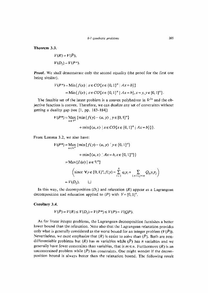
Theorem 3.3.

V(R) = V(F),

V(&) = V(P *) .

Proof. We shall demonstrate only the second equality (the proof for the first one

being similar).

V(P*)=Min{f(x) j XE CO{xe (0, l}” [ Ax=b}}

=Min{f(x> /x~C0{~~{0,1}"~Ax=b},x=y,y~[0, l]“}.

The feasible set of the latest problem is a convex polyhedron in R2N and the ob-

jective function is convex. Therefore, we can dualize any set of constraints without

getting a duality gap (see [l, pp. 183-1841)

v(p*)=~~{min{f(y)-(u,r) IY~W,11”1

+min{(u,x) ~x~C0{~~{0,1}"/Ax=b))}.

From Lemma 3.2, we also have:

Up*) = 2: {min{f(y) - 04 Y> I Y E (0, l>“>

+min{(u,x> 1 Ax=b,x~{O, 1)“))

=Max{L(u) 1 UE IR”)

In this way, the decomposition (Q) and relaxation (R) appear as a Lagrangean

decomposition and relaxation applied to (P) with Y= [0, 11”.

Corollary 3.4.

V(P) = V(R) I V(D2) = l’(P *) I l’(P) = l’(QP).

As for linear integer problems, the Lagrangean decomposition furnishes a better

lower bound than the relaxation. Note also that the Lagrangean relaxation provides

only what is generally considered as the worst bound for an integer problem (V(P)).

Nevertheless, we must emphasize that (R) is easier to solve than (P). Both are non-

differentiable problems but (R) has rn variables while (I’) has n variables and we

generally have fewer constraints than variables, that is msn. Furthermore (R) is an

unconstrained problem while (I’) has constraints. One might wonder if the decom-

position bound is always better than the relaxation bound. The following result

Lagrangean Methods for 0-1 Quadratic Problems

Documents

Transcript of Lagrangean Methods for 0-1 Quadratic Problems