Conditioning of linear-quadratic two-stage stochastic optimization problems

1 23

Mathematical ProgrammingA Publication of the MathematicalOptimization Society ISSN 0025-5610Volume 148Combined 1-2 Math. Program. (2014) 148:201-221DOI 10.1007/s10107-013-0734-0

Conditioning of linear-quadratic two-stagestochastic optimization problems

Konstantin Emich, René Henrion &Werner Römisch

1 23

Your article is protected by copyright and

all rights are held exclusively by Springer-

Verlag Berlin Heidelberg and Mathematical

Optimization Society. This e-offprint is for

personal use only and shall not be self-

archived in electronic repositories. If you wish

to self-archive your article, please use the

accepted manuscript version for posting on

your own website. You may further deposit

the accepted manuscript version in any

repository, provided it is only made publicly

available 12 months after official publication

or later and provided acknowledgement is

given to the original source of publication

and a link is inserted to the published article

on Springer's website. The link must be

accompanied by the following text: "The final

publication is available at link.springer.com”.

Math. Program., Ser. B (2014) 148:201–221DOI 10.1007/s10107-013-0734-0

FULL LENGTH PAPER

Conditioning of linear-quadratic two-stage stochasticoptimization problems

Konstantin Emich · René Henrion ·Werner Römisch

Received: 29 March 2013 / Accepted: 5 December 2013 / Published online: 20 December 2013© Springer-Verlag Berlin Heidelberg and Mathematical Optimization Society 2013

Abstract In this paper a condition number for linear-quadratic two-stage stochasticoptimization problems is introduced as the Lipschitz modulus of the multifunctionassigning to a (discrete) probability distribution the solution set of the problem. Beingthe outer norm of the Mordukhovich coderivative of this multifunction, the conditionnumber can be estimated from above explicitly in terms of the problem data by applyingappropriate calculus rules. Here, a chain rule for the extended partial second-ordersubdifferential recently proved by Mordukhovich and Rockafellar plays a crucial role.The obtained results are illustrated for the example of two-stage stochastic optimizationproblems with simple recourse.

Keywords Stochastic optimization · Two-stage linear-quadratic problems ·Conditioning · Coderivative calculus · Simple recourse

Mathematics Subject Classification 90C15 · 90C31 · 49K40

1 Introduction

In numerical analysis, a condition number of a given mathematical problem representsan upper bound on the ratio of the (relative) solution error to the (relative) data error.

This work was supported by the DFG Research Center Matheon “Mathematics for key technologies” inBerlin.

K. Emich · R. Henrion (B)Weierstrass Institute, Berlin, Germanye-mail: [email protected]

W. RömischHumboldt University, Berlin, Germany

123

Author's personal copy

202 K. Emich et al.

Its size provides information on the difficulty of solving the problem and its reciprocalis often proportional to the perturbation distance of the problem from ill-posedness. In[2] an increasing interest in conditioning of various optimization models is detected(see, for example, [3,8,10,14,23]) and general concepts are developed for derivingcondition numbers of generalized equations.

In this paper, we consider convex stochastic optimization models of the form

min

⎧⎨

⎩

∫

Rs

g(x, ξ)P(dξ) : x ∈ X

⎫⎬

⎭, (1)

where X is a nonempty closed convex subset of Rm, P a probability distribution on

Rs and g is an extended real-valued measurable function on R

m ×Rs such that g(·, ξ)

is convex for all ξ in the support of P . Particular cases of (1) are two-stage linear orlinear-quadratic stochastic programs. Our aim is to derive results on the conditioningof such optimization models.

So far the only paper studying conditioning of such stochastic optimization modelsis [21]. There, the authors assumed for (1) that in addition X is polyhedral, P hasfinite support, g(·, ξ) is piecewise linear for all ξ in the support of P and that (1) has aunique solution x0. Their approach consists in considering empirical or Monte Carlosampling methods for solving (1) and in studying the required sample size N suchthat the unique (random) solution xN of the empirical approximation

min

{

N−1N∑

i=1

g(x, ξ i ) : x ∈ X

}

, (2)

satisfies problem (1) with high probability. The ξ i , i ∈ N, in (2) are independentand identically distributed R

s-valued random samples with common distribution P .Motivated by large deviation techniques they consider the number β > 0 such that

limN→∞ N−1 log (1 − P(xN = x0)) = −β

as a condition measure of problem (1). More precisely, the number (2β)−1 is calledcondition number of (1). Moreover, the authors derived an approximate formula forthe condition number.

In this paper, we study linear-quadratic two-stage stochastic optimization problems(see [17]) and their conditioning. Such problems may be introduced by consideringthe Lagrangian (see also [16])

L(x, z) = 〈c, x〉+ 12 〈x,Cx〉 + E

(〈z, h(ξ)− T (ξ)x〉 − 12 〈z, Bz〉) (x ∈ X, z ∈ Z),

where X and Z are nonempty convex polyhedra in Rm and R

k , respectively, B andC are symmetric and positive semidefinite matrices, c ∈ R

m, h(ξ) is a random vectorin R

k, T (ξ) is a stochastic k × m-matrix, and E denotes expectation with respect to

123


Conditioning of linear-quadratic two-stage 203

a probability distribution P . Primal and dual problems are then associated by generalduality and given by

minx∈X

maxz∈Z

L(x, z) and maxz∈Z

minx∈X

L(x, z).

The primal problem is of the form

min

{

〈c, x〉 + 1

2〈x,Cx〉 + E (�(x, ξ)) |x ∈ X

}

, (3)

where x is the first-stage decision and

�(x, ξ) = maxz∈Z

{

〈z, h(ξ)− T (ξ)x〉 − 1

2〈z, Bz〉

}

. (4)

We assume that a (k, r)-matrix W and a vector q ∈ Rr are given and consider the

following explicit description of the polyhedron Z :

Z = {z ∈ Rk : W �z ≤ q}. (5)

As shown in the “Appendix”, if B is positive definite then (4) may be reformulated as

�(x, ξ)= infy≥0

{

〈q, y〉+ 1

2

⟨h(ξ)−T (ξ)x−W y, B−1(h(ξ)−T (ξ)x−W y)

⟩}

. (6)

Hence, �(x, ξ) corresponds to minimal second stage (random) costs associated witha recourse decision y ∈ R

r taken upon observing ξ ∈ Rs and penalizing the violation

of the equality

W y = h(ξ)− T (ξ)x (7)

by means of a quadratic penalty term instead of meeting (7) exactly as in classicaltwo-stage linear stochastic optimization. The latter would require to assume relativecomplete recourse. In the context of two-stage linear-quadratic stochastic optimizationwe do not insist on this assumption.

As shown in [19, Theorems 9 and 23], solutions of two-stage stochastic programsdo not depend in a Lipschitzian way on the underlying probability distribution ingeneral. More precisely, the behaviour of the growth function

ψP (τ ) = inf

⎧⎨

⎩

∫

Rs

g(x, ξ)P(dξ)− v(P)|d(x, S(P)) ≥ τ, x ∈ X

⎫⎬

⎭(τ ≥ 0) (8)

near τ = 0 has to be studied. Here, v(P) and S(P) are the optimal value and thesolution set of (1), respectively, and d(x, S(P)) refers to the distance of x ∈ X toS(P). Lipschitzian dependence can be concluded if the functionψP has linear growth

123


204 K. Emich et al.

close to τ = 0 or ifψP has quadratic growth and a Lipschitz stability argument due to[20] (see also [1, Section 4.4.1]) is employed. If the support of P is finite, two-stagelinear stochastic programs satisfy a linear growth condition and two-stage linear-quadratic stochastic programs a quadratic growth condition, respectively. Indeed, weprovide a calmness result for solutions in the latter case (see Proposition 3.2).

Therefore, we assume that the random vector ξ has a discrete uniform probabilitydistribution with atoms or scenarios ξ1, . . . , ξ N . Then the optimization problem (3)can be written as

min

{

〈c, x〉 + 1

2〈x,Cx〉 + N−1

N∑

i=1

�(x, ξ i )|x ∈ X

}

. (9)

In order to study the dependence of solutions to (9) on the probability distributionwe consider the vector p := (

ξ1, . . . , ξ N)

of scenarios and introduce the solution setmapping S : R

Ns ⇒ Rm as

S(p) := {x ∈ X |x solves (9)}. (10)

Our aim is to apply concepts from [2] in order to associate a condition number withthe two-stage stochastic optimization problem (9).

2 Basic concepts and notation

As usual, we denote by ‘gr M’ the graph of some multifunction M . Denote by Bδ(y)the closed ball of radius δ around some y in a metric space. We recall the followingtwo basic properties of multifunctions M : X ⇒ Y between metric spaces X,Y :

Definition 2.1 M has the Aubin property at a point (x, y) ∈ gr M if there existL , δ > 0 such that

d (y,M (x1)) ≤ Ld (x1, x2) ∀x1, x2 ∈ Bδ(x), ∀y ∈ [M (x2) ∩ Bδ(y)] . (11)

As a weaker condition, M is said to be calm at (x, y) ∈ gr M if there exist L , δ > 0such that

d (y,M (x)) ≤ Ld (x, x) ∀x ∈ Bδ(x), ∀y ∈ [M (x) ∩ Bδ(y)] .

The constant

lip M(x, y) := inf {L|∃δ > 0 : (11)} (12)

is called the graphical modulus of M at (x, y) [18, p. 377]. It can be interpreted as theLipschitz modulus of the multifunction M . For the following definitions and propertieswe refer the reader to [12] and [18].

123



Definition 2.2 Let C ⊆ Rm be a closed subset and x ∈ C . The Mordukhovich normal

cone to C at x is defined by

NC (x) :={

x∗|∃ (xn, x∗

n

) → (x, x∗) : xn ∈ C, x∗

n ∈ [TC (xn)]0}.

Here, [TC (xn)]0 refers to the Fréchet normal cone to C at xn , which is the negativepolar of the contingent cone

TC (x) := {d ∈ R

m |∃tk ↓ 0, dk → d : x + tkdk ∈ C,∀k}. (13)

to C at xn . For an extended-real-valued, lower semicontinuous function f : Rm → R

with | f (x)| < ∞, the Mordukhovich normal cone induces a subdifferential via

∂ f (x) := {x∗| (x∗,−1

) ∈ Nepi f (x, f (x))}.

If f : Rm → R is locally Lipschitz around x and g : R

m → R is proper and lowersemicontinuous with |g(x)| < ∞, then the following sum rule applies:

∂ ( f + g) (x) ⊆ ∂ f (x)+ ∂g(x). (14)

Definition 2.3 Let M : Rn ⇒ R

m be a multifunction with closed graph. The Mor-dukhovich coderivative D∗M(x, y) : R

m ⇒ Rn of M at some (x, y) ∈ gr M is

defined as

D∗M(x, y)(y∗) := {x∗ ∈ R

n| (x∗,−y∗) ∈ Ngr M (x, y)}

When M is single-valued, i.e., y = M(x), we simply write D∗M(x) instead ofD∗M(x,M(x)).

If f : Rm → R is locally Lipschitz around x , then the following scalarization formula

holds true:

D∗ f (x)(y∗) = ∂⟨y∗, f

⟩(x). (15)

Definition 2.4 Let f : Rn → R ∪ {∞} be a lower semicontinuous function which is

finite at x ∈ Rn . For an element u ∈ ∂ f (x), the second-order subdifferential of f at

(x, u) is a multifunction ∂2 f (x, u) : Rn ⇒ R

n defined by

∂2 f (x, u) (w) := (D∗∂ f

)(x, u) (w) ∀w ∈ R

n .

If ∂ f (x) is single-valued, then, similar to Definition 2.3, we simply write ∂2 f (x).

Definition 2.5 Let f : Rn × R

m → R ∪ {∞} be a lower semicontinuous func-tion which is finite at (x, z) ∈ R

n × Rm . The partial subdifferential is defined

as ∂x f (x, z) := ∂ f (·, z) (x). Following [13], for (x, z) ∈ Rn × R

m and any

123


206 K. Emich et al.

u ∈ ∂x f (x, z), the (extended) partial second-order subdifferential of f is a multi-function ∂2

x f (x, z, u) : Rn ⇒ R

n × Rm defined by

∂2x f (x, z, u) (w) := (

D∗∂x f)(x, z, u) (w) ∀w ∈ R

n .

If ∂x f (x, z) is single-valued, then, similar to Definition 2.3, we simply write ∂2x f (x, z).

3 A condition number for linear-quadratic two-stage stochastic optimizationproblems

We consider the representation (4) of the optimal second-stage costs with the polyhe-dron Z defined in (5):

�(x, ξ) = supz

{

〈h(ξ)− T (ξ)x, z〉 − 1

2〈z, Bz〉 |W �z ≤ q

}

Throughout the rest of the paper we shall make the following assumptions for �:

• B is symmetric and positive definite.• The polyhedron Z is nonempty and its description (5) satisfies the Linear Indepen-

dence Constraint Qualification (i.e., at each point of Z the active rows of the matrixW T are linearly independent).

• T and h are continuously differentiable.

As a consequence of these assumptions, � is finite-valued and �(·, ξ) is convex forany ξ ∈ R

s . Now, the solution set to our optimization problem (9) is equivalentlycharacterized by the generalized equation

0 ∈ ∂x(x, p)+ NX (x), (16)

where ∂x and N denote the partial subdifferential and the normal cone, respectively,in the sense of convex analysis and

(x, p) := 〈c, x〉 + 1

2〈x,Cx〉 + N−1

N∑

i=1

�(x, ξ i )

×(

x ∈ Rm, p =

(ξ1, . . . , ξ N

)∈ R

Ns). (17)

Consequently, the solution set mapping S defined in (10) can also be written as

S(p) = {x ∈ Rm | (16) is satisfied}. (18)

Following [2], we call lip S ( p, x) as defined in (12) the condition number of problem(9) at a point ( p, x) ∈ gr S. By definition, lip S ( p, x) < ∞ if and only if S has

123



the Aubin property at ( p, x) (see Definition 2.1). Moreover [18, Theorem 9.40], thecondition number can be calculated as

lip S ( p, x) = supx∗∈B

supp∗∈D∗S( p,x)(x∗)

∥∥p∗∥∥ , (19)

where D∗S ( p, x) refers to the Mordukhovich coderivative of S at ( p, x) (see Defini-tion 2.3). We also recall the well-known Mordukhovich criterion [11, Theorem 5.7]stating that S has the Aubin property at ( p, x) if and only if D∗S ( p, x) (0) = 0.

The following observation follows from standard results of parametric nonlinearprogramming (see, e.g., [1, Remark 4.14]) via the positive definiteness of B and theLinear Independence Constraint Qualification for Z :

Proposition 3.1 Let (x, ξ ) ∈ Rm × R

s be arbitrary. Then, the function � is Fréchetdifferentiable with ∇x�(x, ξ ) = −T �(ξ )z(h(ξ )− T (ξ )x), where z(v) is the uniqueelement of

argmaxW�z≤q

〈v, z〉 − 12 〈z, Bz〉. (20)

Moreover, since z(·) is locally Lipschitz, ∇x� is locally Lipschitz too around (x, ξ ).

Corollary 3.1 Let x ∈ Rm and p = (

ξ1, . . . , ξ N) ∈ R

Ns. Then, the partial gradient∇x(x, p) of the function defined in (17) exists, is Lipschitz continuous around(x, p) and is given by

∇x(x, p) = c + Cx + N−1N∑

i=1

∇x�(x, ξi ).

In other words, (9) is a C1,1 optimization problem. Using Corollary 3.1 we are able toshow that the assumptions on � imply upper Lipschitz continuity and, in particular,calmness of S (see Definition 2.1).

Proposition 3.2 Let X be bounded. The solution set mapping S defined in (18) isupper Lipschitz continuous at any p ∈ dom S, i.e., it holds

supx∈S(p)

d(x, S( p)) ≤ L

c‖p − p‖ (p ∈ V ), (21)

where the constant c > 0 appears in the quadratic growth condition

(x, p)−(x, p) ≥ c d(x, S( p))2 (x ∈ X ∩ U ), (22)

U and V are bounded neighborhoods of x and p, respectively and L > 0 a localLipschitz constant of ∇x(·, ·) on U × V .

123


208 K. Emich et al.

Proof Let (x, p) ∈ gr S. The objective function (·, p) is convex piecewise linear-quadratic and, hence, satisfies a quadratic growth condition due to [9, Theorem 2.7].Hence, there exist a bounded neighborhood U of S( p) and a constant c > 0 such that(22) holds. Since is continuous and X is compact, the solution set mapping is uppersemicontinuous at P (see, for example, [1, Proposition 4.4]). Hence, there exists abounded neighborhood V ′ of p such that S(p) ⊆ U if p ∈ V ′. Next we make use ofthe results in [1, Section 4.4.1] on Lipschitz stability of nonlinear programs in case ofa fixed feasible set and obtain

d(x, S( p)) ≤ 1

csupy∈U

‖∇x(y, p)− ∇x(y, p)‖

for any x ∈ S(p) and p in some neighborhood V contained in V ′. From Corollary 3.1we conclude that (21) is true. ��For more general results on the stability of solutions to C1,1 problems we refer, e.g.,to [6,7].

Now we are in a position to formulate an upper estimate for the coderivative ofour solution mapping S in (18) as it will be required in an upper estimation of thecondition number (19):

Proposition 3.3 Let ( p, x) ∈ gr S, where x ∈ X and p := (ξ1, . . . , ξ N

) ∈ RNs.

Assume that the multifunction

M(w) := {(p, x) |w ∈ ∇x(x, p)+ NX (x)} (23)

is calm at (0, p, x) (see Definition 2.1). Then,

D∗S ( p, x)(x∗) ⊆

{p∗|∃v∗ : (−x∗, p∗) ∈ ∂2

x (x, p)(v∗)

+D∗NX (x,−∇x (x, p))(v∗) × {0}

}. (24)

Proof By Corollary 3.1, there exists a neighbourhood U of (x, p) such that the solutionmapping S is locally described by

S(p) = {x |0 ∈ f (x, p)+ NX (x)} ∀(x, p) ∈ U ,

where f (x, p) := ∇x(x, p) is Lipschitz on U . From the equivalence

(p, x) ∈ gr S ⇐⇒ g(p, x) := (x,− f (x, p)) ∈ gr NX (25)

we see that gr S = g−1 (gr NX ) for a locally Lipschitzian mapping g. As observed in[22, Proposition 5.2] , our calmness assumption implies calmness of the multifunction

w := (w1, w2) �→ {(p, x) |w2 − ∇x(x, p) ∈ NX (x + w1)}= {(p, x) |g(p, x)+ w ∈ gr NX }

123



at (0, 0, p, x). This allows us to invoke [4, Theorem 4.1], in order to derive from (25)the inclusion

Ngr S ( p, x) ⊆⋃{

D∗g ( p, x)(w∗) |w∗ ∈ Ngr NX (g ( p, x))

}. (26)

With the partition w∗ = (u∗, v∗) and defining the functions π (p, x) := x and

f (p, x) := − f (x, p) we obtain that g =(π, f

)and, thus,

D∗g ( p, x)(u∗, v∗) = ∂

⟨w∗, g

⟩( p, x) = ∂

(⟨u∗, π

⟩ +⟨v∗, f

⟩)( p, x)

⊆ ∂⟨u∗, π

⟩( p, x)+ ∂

⟨v∗, f

⟩( p, x)

= (0, u∗) + D∗ f ( p, x)

(v∗).

Here we exploited the sum rule (14) and the scalarization formula (15). Moreover,using the definition of the coderivative it is easy to see by virtue of [18, Exercise 6.7]that

(x∗, p∗) ∈ D∗ f (x, p)

(−v∗) ⇐⇒ (p∗, x∗) ∈ D∗ f ( p, x)

(v∗).

As a consequence,

D∗g ( p, x)(u∗, v∗) ⊆ {(

p∗, x∗) | (x∗ − u∗, p∗) ∈ D∗ f (x, p)(−v∗)}.

Combining this with (26) yields

D∗S ( p, x)(x∗) ⊆ {

p∗|∃ (u∗, v∗) ∈ Ngr NX (g ( p, x)) : (−x∗ − u∗, p∗)

∈ D∗ f (x, p)(−v∗)}

which leads to (24) upon recalling the definitions of g and f as well as the fact thatD∗∇x (x, p) = ∂2

x (x, p) (see Definition 2.5). ��

4 Computation of ∂2x�

In order to apply Proposition 3.3, we have to compute explicitly the partial second-order subdifferential ∂2

x (explicit formulae for the other term D∗NX are availablefrom the literature, see, e.g., [5]). As a first step, we reduce the computation of ∂2

x

to that of ∂2x�:

Proposition 4.1 Under the assumption of Proposition 3.3 holding at some ( p, x) ∈gr S, where x ∈ X and p := (

ξ1, . . . , ξ N) ∈ R

Ns one gets that, for all v∗ ∈ Rm,

123


210 K. Emich et al.

∂2x (x, p)

(v∗) ⊆

{(

C�v∗ + N−1N∑

i=1

x∗i , N−1 p∗

)

| (x∗i , p∗

i

) ∈ ∂2x�

×(

x, ξ i) (v∗) (i = 1, . . . , N )

}

.

Proof Defining p := (ξ1, . . . , ξ N

)and �i (x, p) := �

(x, ξ i

)for i = 1, . . . , N and

(x, p) in a neighbourhood of (x, p), we may write �i = � ◦ ϑi , where ϑi (x, p) =(x, ξ i

)and infer that ∇x�i = (∇x�) ◦ Ai with a surjective matrix

Ai :=(

I 00 Bi

)

; Bi :=(

0, . . . , 0, Ii, 0, . . . , 0

)

.

Now, the coderivative chain rule in [12, Theorem 1.66] yields that

D∗∇x�i (x, p) =[

Ai]�

D∗∇x�(

x, ξ i)

=[

Ai]�∂2

x�(

x, ξ i)

(i = 1, . . . , N ) .

On the other hand, ∇x (x, p) = c+Cx+N−1 ∑Ni=1 ∇x�i (x, p) by (17). Therefore,

exploiting Definition 2.5 and the calculus rules (14) and (15), one ends up with

∂2x (x, p)

(v∗) = D∗∇x(x, p)

(v∗) = ∂

⟨v∗,∇x

⟩(x, p) ⊆

(C�v∗, 0

)

+ N−1N∑

i=1

∂⟨v∗,∇x�i

⟩(x, p)

=(

C�v∗, 0)

+ N−1N∑

i=1

D∗∇x�i (x, p)(v∗) =

(C�v∗, 0

)

+ N−1N∑

i=1

[Ai

]�∂2

x�(

x, ξ i) (v∗) .

Consequently, we arrive at the assertion of our Proposition via the inclusion

∂2x (x, p)

(v∗) ⊆

{(

C�v∗, 0)

+ N−1N∑

i=1

(x∗

i , B�i p∗

i

)| (x∗

i , p∗i

)

∈ ∂2x�

(x, ξ i

) (v∗) (i = 1, . . . , N )

}

.

��After reducing ∂2

x to ∂2x� we are now faced with the computation of the latter. In

order to do so, it will be convenient to write � in (4) as a composition

123



�(x, ξ)=θ (α(x, ξ)) , α(x, ξ) :=h(ξ)− T (ξ)x, θ (v) := supW�z≤q

〈v, z〉− 12 〈z, Bz〉

(27)

Now, a chain rule for partial second-order subdifferentials recently proved by Mor-dukhovich and Rockafellar [13, Theorem 3.1] allows us to derive the following furtherreduction:

Lemma 4.1 Let x ∈ Rm and ξ ∈ R

s be such that T (ξ ) is surjective. Then, for allv∗ ∈ R

m, it holds that

∂2x�

(x, ξ

) (v∗) = −

(0,∇� ⟨

z(α(x, ξ )

), T (·) v∗⟩ (ξ

))

+ (−T (ξ ),∇h(ξ) − ∇ (T (·) x)

(ξ))�

∂2θ(α(x, ξ )

) (−T (ξ )v∗),

where z (v) was introduced in Proposition 3.1.

Proof The surjectivity of ∇xα(x, ξ ) = −T (ξ ) allows us to apply the above-mentionedchain rule in order to derive that

∂2x�

(x, ξ

) (v∗) =

(∇2

xx 〈z, α〉 (x, ξ)v∗,∇2

xξ 〈z, α〉 (x, ξ)v∗)

+ (∇xα(x, ξ

),∇ξ α

(x, ξ

))�∂2θ

(α(x, ξ

), z

) (∇xα(x, ξ

)v∗),

where z is uniquely defined by the equation

∇x�(x, ξ

) = [∇xα(x, ξ

)]�z = −T �(ξ )z.

Hence, z = z(α(x, ξ )

), where z (v) was introduced in Proposition 3.1 as unique

element of (20). Since also

∇x�(x, ξ

) = −T �(ξ )∇θ (α (x, ξ

))

by (27), the injectivity of −T �(ξ ) yields that z = ∇θ (α (x, ξ

))which allows us to

omit the argument z in the expression ∂2θ(α(x, ξ

), z

). Taking into account that

∇2xx 〈z, α〉 (x, ξ

)v∗ = 0

∇2xξ 〈z, α〉 (x, ξ

)v∗ = − [∇ ⟨

z, T (·) v∗⟩ (ξ)]�

∇ξα(x, ξ

) = ∇h(ξ) − ∇ (T (·) x)

(ξ),

we arrive at the asserted formula. ��Now, it remains to provide an explicit formula for the second order subdifferential∂2θ . Before doing so, we recall the following

123


212 K. Emich et al.

Proposition 4.2 [5, Corollary 3.5] Consider a polyhedron P := {u|Au ≤ b}. Fixarbitrary u ∈ P and w ∈ NP (u). Denote by I := {i | 〈ai , u〉 = bi } the index setof active rows of A at u. Assume that these active rows are linearly independent.Moreoever, let J := {i ∈ I |λi > 0} be the index set of strictly positive multipliers,where λ is the unique solution of

∑i∈I λi ai = w. Then,

D∗NP (u, w)(s∗)

={

pos {ai |i ∈ I : 〈ai , s∗〉 > 0} + span {ai |i ∈ I : 〈ai , s∗〉 = 0} if s∗ ∈ ⋂

i∈Ja⊥

i

∅ else.

Here, ‘pos’ and ‘span’ refer to the convex cone and linear subspace, respectively,generated by the elements in the corresponding set.

Proposition 4.3 For any v, w∗ ∈ Rr , the second-order subdifferential of the function

θ in (27) calculates as

∂2θ (v)(w∗) = {

z∗|Bz∗ − w∗ ∈ D∗NZ (z (v) , v − B z (v))(−z∗)}

=

⎧⎪⎪⎨

⎪⎪⎩

{z∗|Bz∗ − w∗ ∈ pos {wi |i ∈ I : 〈wi , z∗〉 < 0}+ span {wi |i ∈ I : 〈wi , z∗〉 = 0}} if z∗ ∈ ⋂

i∈Jw⊥

i

∅ else

where z (v) refers to the unique element of (20) and—with respect to the nota-tion introduced in (5)—the wi represent the columns of the matrix W . MoreoverI := {i | 〈wi , z (v)〉 = qi } is the index set of active rows of W � at z (v) andJ := {i ∈ I |λi > 0} is the index set of strictly positive multipliers, where λ denotesthe unique solution of

∑i∈I λiwi = v − B z (v).

Proof Given the definition of θ in (27) and applying Proposition 3.1 to the specialcase h(ξ) = 0 and T (ξ) = −I for all ξ , we see that θ is strictly differentiable with∇θ(v) being the unique element of (20), i.e., ∇θ(v) = z(v). Moreover, ∇θ is locallyLipschitz. With Z defined in (5), we deduce from (20) the equivalence

(v, z) ∈ gr ∇θ ⇐⇒ v − Bz ∈ NZ (z) ⇐⇒ (z, v − Bz) ∈ gr NZ .

Hence gr ∇θ = L−1gr NZ , where L(v, z) = (z, v − Bz) is a surjective linear map-ping. Then, recalling the symmetry of B, [18, Exercise 6.7] yields that

Ngr ∇θ (v,∇θ (v)) =(

0 II −B

)

Ngr NZ (∇θ (v) , v − B ∇θ (v)).

Exploiting the corresponding definitions, this last relation entails the first equal-ity asserted in this proposition. Now, with Z defined in (5) satisfying the Lin-ear Independence Constraint Qualification (see basic assumptions imposed at thebeginning of Sect. 3), the assertion of the proposition follows immediately fromProposition 4.2. ��

123



5 An upper estimate for the condition number

5.1 An upper estimate for D∗S

Collecting the results of Propositions 3.3, 4.1 and Lemma 4.1, we arrive at the followingupper estimate for the coderivative of the solution mapping S in (18):

Theorem 5.1 Let ( p, x) ∈ gr S, where x ∈ X and p := (ξ1, . . . , ξ N

) ∈ RNs.

Assume that the multifunction (23) is calm at (0, p, x) and that the matrices T (ξ i )

are surjective for i = 1, . . . , N. Then,

D∗S ( p, x)(x∗)

⊆

⎧⎪⎪⎪⎪⎪⎪⎪⎪⎪⎪⎪⎪⎪⎨

⎪⎪⎪⎪⎪⎪⎪⎪⎪⎪⎪⎪⎪⎩

p∗

∣∣∣∣∣∣∣∣∣∣∣∣∣∣∣∣∣∣∣

∃v∗∃u∗ ∈ D∗NX (x,−∇x (x, p))(v∗),

∃z∗i ∈ ∂2θ

(h(ξ i )− T (ξ i )x

) (−T (ξ i )v∗) (i = 1, . . . , N ) :

N−1N∑

i=1

[T (ξ i )

]�z∗

i = C�v∗ + x∗ + u∗,

p∗i = N−1

(

−∇�⟨zi , T (·)v∗⟩(ξ i)

+[∇h

(ξ i)

− ∇(T (·)x)(ξ i)]�

z∗i

)

(i = 1, . . . , N ) ,

⎫⎪⎪⎪⎪⎪⎪⎪⎪⎪⎪⎪⎪⎪⎬

⎪⎪⎪⎪⎪⎪⎪⎪⎪⎪⎪⎪⎪⎭

where the zi are the unique elements of

argmaxW�z≤q

⟨h(ξ i )− T (ξ i )x, z

⟩− 1

2〈z, Bz〉 (i = 1, . . . , N ).

Proof Proposition 3.3 yields that

D∗S ( p, x)(x∗) ⊆

{

p∗|∃v∗, ∃u∗ ∈ D∗NX (x,−∇x (x, p))(v∗) :

(−x∗ − u∗p∗

)

∈ ∂2x (x, p)

(v∗)

}

.

Next, Proposition 4.1 implies that for i = 1, . . . , N there exist(α∗

i , β∗i

) ∈∂2

x�(x, ξ i

)(v∗) such that

C�v∗ + x∗ + u∗ = −N−1N∑

i=1

α∗i

p∗i = N−1β∗

i (i = 1, . . . , N ) .

123


214 K. Emich et al.

Finally, by Lemma 4.1, for i = 1, . . . , N there exist z∗i ∈ ∂2θ

(h(ξ i )− T (ξ i )x

)

(−T (ξ i )v∗) with

α∗i = −

[T (ξ i )

]Tz∗

i

β∗i = −∇T ⟨

zi , T (·) v∗⟩ (ξ i )+[∇h(ξ i )− ∇ (T (·) x)

]Tz∗

i .

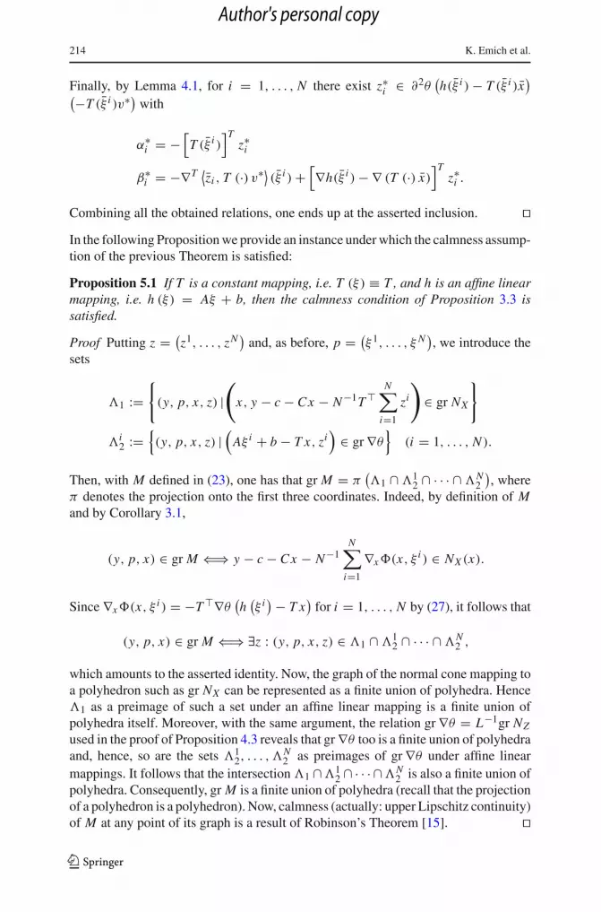
Combining all the obtained relations, one ends up at the asserted inclusion. ��In the following Proposition we provide an instance under which the calmness assump-tion of the previous Theorem is satisfied:

Proposition 5.1 If T is a constant mapping, i.e. T (ξ) ≡ T , and h is an affine linearmapping, i.e. h (ξ) = Aξ + b, then the calmness condition of Proposition 3.3 issatisfied.

Proof Putting z = (z1, . . . , zN

)and, as before, p = (

ξ1, . . . , ξ N), we introduce the

sets

�1 :={

(y, p, x, z) |(

x, y − c − Cx − N−1T �N∑

i=1

zi

)

∈ gr NX

}

�i2 :=

{(y, p, x, z) |

(Aξ i + b − T x, zi

)∈ gr ∇θ

}(i = 1, . . . , N ).

Then, with M defined in (23), one has that gr M = π(�1 ∩�1

2 ∩ · · · ∩�N2

), where

π denotes the projection onto the first three coordinates. Indeed, by definition of Mand by Corollary 3.1,

(y, p, x) ∈ gr M ⇐⇒ y − c − Cx − N−1N∑

i=1

∇x�(x, ξi ) ∈ NX (x).

Since ∇x�(x, ξ i ) = −T �∇θ (h (ξ i) − T x

)for i = 1, . . . , N by (27), it follows that

(y, p, x) ∈ gr M ⇐⇒ ∃z : (y, p, x, z) ∈ �1 ∩�12 ∩ · · · ∩�N

2 ,

which amounts to the asserted identity. Now, the graph of the normal cone mapping toa polyhedron such as gr NX can be represented as a finite union of polyhedra. Hence�1 as a preimage of such a set under an affine linear mapping is a finite union ofpolyhedra itself. Moreover, with the same argument, the relation gr ∇θ = L−1gr NZ

used in the proof of Proposition 4.3 reveals that gr ∇θ too is a finite union of polyhedraand, hence, so are the sets �1

2, . . . , �N2 as preimages of gr ∇θ under affine linear

mappings. It follows that the intersection�1 ∩�12 ∩ · · · ∩�N

2 is also a finite union ofpolyhedra. Consequently, gr M is a finite union of polyhedra (recall that the projectionof a polyhedron is a polyhedron). Now, calmness (actually: upper Lipschitz continuity)of M at any point of its graph is a result of Robinson’s Theorem [15]. ��

123



Combining Proposition 5.1 with Theorem 5.1 and Proposition 4.3, we may draw thefollowing conclusion for a simplified setting:

Corollary 5.1 Let ( p, x) ∈ gr S, where x ∈ X and p := (ξ1, . . . , ξ N

) ∈ RNs.

Assume that T (ξ) ≡ T , and h (ξ) = Aξ + b. Moreover, let T be surjective. Then,

D∗S ( p, x)(x∗)

⊆

⎧⎪⎪⎪⎪⎪⎪⎪⎪⎪⎨

⎪⎪⎪⎪⎪⎪⎪⎪⎪⎩

p∗

∣∣∣∣∣∣∣∣∣∣∣∣∣∣∣

∃v∗, ∃u∗ ∈ D∗NX (x,−c − Cx + N−1T �N∑

i=1

z(vi ))(v∗)

∃z∗i : Bz∗

i + T v∗ ∈ D∗NZ (z(vi ), vi − Bz(vi ))(−z∗i ) (i = 1, . . . , N )

N−1T �N∑

i=1

z∗i = C�v∗ + x∗ + u∗

p∗i = N−1 A�z∗

i , vi = Aξ i + b − T x (i = 1, . . . , N )

⎫⎪⎪⎪⎪⎪⎪⎪⎪⎪⎬

⎪⎪⎪⎪⎪⎪⎪⎪⎪⎭

(28)

where z(v) is defined in (20).

Hence, D∗S ( p, x) (x∗) is contained in a set which is given in terms of the data ofthe stochastic program and of the Mordukhovich coderivative of the normal conemappings to the polyhedra X and Z , respectively. The latter may be computed byProposition 4.2.

5.2 Application to conditioning in the case of simple recourse

We apply the result of the previous section to the special setting of so-called sim-ple recourse. More precisely, we assume that our two-stage stochastic optimizationproblem has the following (primal) form:

minx∈X

〈c, x〉 + σ

2‖x‖2 + N−1

N∑

i=1

�(x, ξ i ),

where ξ i ∈ Rs (i = 1, . . . , N ) are realizations of the random vector ξ and where

X := {x ∈ R

m |Dx ≤ f}

�(x, ξ) := sup−q−≤z≤q+

〈Aξ + b − T x, z〉 − τ

2‖z‖2 .

We assume that τ, σ > 0. Note that this problem differs from a standard problemof simple recourse type as much as our general problem (9) differs from a standardtwo-stage problem by admitting violation of recourse at the cost of a penalty. Thereason to use the term ’simple recourse’ here, is the rectangular shape of the set Z in(5). Clearly, this problem fits the model (9) with

123


216 K. Emich et al.

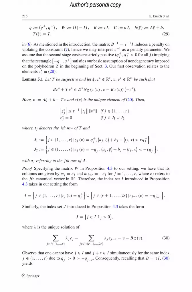
q := (q+, q−) , W := (I | − I ) , B := τ I, C := σ I, h(ξ) := Aξ + b,

T (ξ) ≡ T . (29)

in (6). As mentioned in the introduction, the matrix B−1 = τ−1 I induces a penalty onviolating the constraint (7), hence we may interpret τ−1 as a penalty parameter. Weassume that the second stage costs are strictly positive (q+

j , q−j > 0 for all j) implying

that the rectangle[−q−, q+] satisfies our basic assumption of nondegeneracy imposed

on the polyhedron Z in the beginning of Sect. 3. Our first observation relates to theelements z∗

i in (28):

Lemma 5.1 Let T be surjective and let ξ, z∗ ∈ Rr , x, v∗ ∈ R

m be such that

Bz∗ + T v∗ ∈ D∗NZ (z (v) , v − B z(v))(−z∗).

Here, v := Aξ + b − T x and z(v) is the unique element of (20). Then,

∣∣∣z∗

j

∣∣∣ ≤ τ−1

∥∥t j

∥∥ ‖v∗‖ if j ∈ {1, . . . , r}

z∗j = 0 if j ∈ J1 ∪ J2

where, t j denotes the j th row of T and

J1 :={

j ∈ {1, . . . , r} |z j (v) = q+j ,

⟨a j , ξ

⟩ + b j − ⟨t j , x

⟩> τq+

j

}

J2 :={

j ∈ {1, . . . , r} |z j (v) = −q−j ,

⟨a j , ξ

⟩ + b j − ⟨t j , x

⟩< −τq−

j

},

with a j referring to the j th row of A.

Proof Specifying the matrix W in Proposition 4.3 to our setting, we have that itscolumns are given by w j = e j and w j+r = −e j for j = 1, . . . , r , where e j refers tothe j th canonical vector in R

r . Therefore, the index set I introduced in Proposition4.3 takes in our setting the form

I ={

j ∈ {1, . . . , r} |z j (v) = q+j

}∪{

j ∈ {r + 1, . . . , 2r} |z j−r (v) = −q−j−r

}.

Similarly, the index set J introduced in Proposition 4.3 takes the form

J = {j ∈ I |λ j > 0

},

where λ is the unique solution of

∑

j∈I∩{1,...,r}λ j e j −

∑

j∈I∩{r+1,...,2r}λ j e j−r = v − B z (v). (30)

Observe that one cannot have j ∈ I and j + r ∈ I simultaneously for the same indexj ∈ {1, . . . , r} due to q+

j > 0 > −q−j−r . Consequently, recalling that B = τ I , (30)

yields

123



λ j = v j − τ z j (v) = v j − τq+j if j ∈ I ∩ {1, . . . , r}

−λ j = v j−r − τ z j−r (v) = v j−r + τq−j−r if j ∈ I ∩ {r + 1, . . . , 2r}

It follows that

J ={

j ∈ {1, . . . , r} |z j (v) = q+j ,

⟨a j , ξ

⟩ + b j − ⟨t j , x

⟩> τq+

j

}

∪{

j ∈ {r + 1, . . . , 2r} |z j−r (v) = −q−j−r ,

⟨a j−r , ξ

⟩ + b j−r − ⟨t j−r , x

⟩< −τq−

j−r

}

Now, by Proposition 4.3,⟨z∗, w j

⟩ = 0 for all j ∈ J . With respect to the indexsets J1, J2 introduced in the statement of this Lemma, the following holds true: Ifj ∈ J1, then j belongs to the first set in the union above, hence j ∈ J . Then,0 = ⟨

z∗, w j⟩ = z∗

j . Similarly, if j ∈ J2, then j + r belongs to the second set in the

union above, hence j + r ∈ J . Then, 0 = ⟨z∗, w j+r

⟩ = −z∗j . This proves the second

statement in the assertion of this Lemma. Next, let j ∈ {1, . . . , r} be arbitrary. Therelation Bz∗ + T v∗ ∈ D∗NZ (z (v) , v − B z(v) (−z∗) translates by Proposition 4.3in our setting to

τ z∗ + T v∗ ∈ pos{w j | j ∈ I : ⟨w j , z∗⟩ < 0

} + span{w j | j ∈ I : ⟨w j , z∗⟩ = 0

}

or to

τ z∗ + T v∗ =∑

k≤r,k∈I,z∗k<0

λak ek −

∑

k≤r,k+r∈I,z∗k>0

λbkek +

∑

k≤r,k∈I,z∗k =0

μak ek

+∑

k≤r,k+r∈I,z∗k =0

μbkek (31)

for certain coefficients λak , λ

bk ≥ 0 and μa

k , μbk ∈ R. Now, if z∗

j = 0, then the estimatein the first statement in the assertion of our Lemma is trivially satisfied. Otherwise, ifz∗

j �= 0, then by (31),

τ z∗j + ⟨

t j , v∗⟩ =

⎧⎨

⎩

λaj ≥ 0 if j ∈ I, z∗

j < 0−λb

j ≤ 0 if j + r ∈ I, z∗j > 0

0 else.

In the first case, one has that 0 > z∗j ≥ −τ−1

⟨t j , v

∗⟩ which directly implies the

asserted estimate∣∣∣z∗

j

∣∣∣ ≤ τ−1

∥∥t j

∥∥ ‖v∗‖. The second case follows analogously. The

third case is evident as well. This proves the first statement in the assertion of thisLemma. ��Observe that the index sets J1, J2 introduced in Lemma 5.1 represent those componentsj of the solution z (v) of problem (20) for v := Aξ+b−T x which are strongly active(i.e., which are active with respect to the constraints −q− ≤ z ≤ q+ and for whichthe associated Lagrange multiplier is strictly positive). This Lemma eventually allows

123


218 K. Emich et al.

us to calculate an upper estimate for the condition number in case of simple recourse.To this aim, we fix some x ∈ X and p := (

ξ1, . . . , ξ N) ∈ R

Ns such that x ∈ S ( p),i.e., 0 ∈ ∇x(x, p) + NX (x) for defined in (17). With di referring to the rows ofD in the description Dx ≤ f of the polyhedron X , this implies that

∇x(x, p) =∑

i∈ I

λi di

(I := {i | 〈di , x〉 = fi }

)(32)

for certain λi ≤ 0(

i ∈ I)

. For each i = 1, . . . , N we put vi := Aξ i + b − T x and

introduce the index sets

J1(i) :={

j ∈ {1, . . . , r} |z j

(vi)

= q+j ,

⟨a j , ξ

i⟩+ b j − ⟨

t j , x⟩> τq+

j

}

J2(i) :={

j ∈ {1, . . . , r} |z j

(vi)

= −q−j ,

⟨a j , ξ

i⟩+ b j − ⟨

t j , x⟩< −τq−

j

},

i.e., the same index sets characterizing strongly active components in the solution ofproblem (20) as in Lemma 5.1 but now related to the different scenarios ξ i . This allowsus to define the following quantity

�(T ) :=N∑

i=1

�i (T ), �i (T ) :=⎛

⎝∑

j∈{1,...,r}\(J1(i)∪J2(i))

∥∥t j

∥∥2

⎞

⎠

1/2

(i = 1, . . . , N ) .

Observe that �(T ) increases not only with increasing elements of the matrix T butalso with decreasing number of strongly active components in the scenario-dependentsolutions z (vi ) of the problems

max−q−≤z≤q+ 〈vi , z〉 − τ

2‖z‖2 . (33)

Clearly, 0 ≤ �i (T ) ≤ ‖T ‖F , where ‖·‖F refers to the Frobenius norm. Here, theminimum is attained if all components of z (vi ) are strongly active (i.e., z (vi ) equals acorner of the rectangle

[−q−, q+] and all Lagrange multipliers are strictly positive).In contrast, the maximum is attained if no component is strongly active (e.g., z (vi ) liesin the interior of the rectangle

[−q−, q+] or it lies on the boundary of this rectanglebut all Lagrange multipliers equal zero). We have the following upper estimate for thecondition number:

Theorem 5.2 In the setting specified above, assume that even λi < 0(

i ∈ I)

in (32),

i.e., strict complementarity holds at x . Moreover, let T be surjective. Finally, let theparameters σ and τ in (29) satisfy the relation

τσ > N−1 ‖T ‖�(T ). (34)

123



Then, the condition number lip S ( p, x) as introduced in (19), can be estimated by

lip S ( p, x) ≤ ‖A‖([�(T )]−1 Nστ − ‖T ‖) .

Proof In order to estimate lip S ( p, x), fix an arbitrary x∗ with ‖x∗‖ ≤ 1 andan arbitrary p∗ ∈ D∗S ( p, x) (x∗). Our assumptions allow us to apply Corollary5.1. Accordingly, there exist u∗, v∗ and z∗

i satisfying the relations in (28). In par-

ticular, u∗ ∈ D∗NX

(x,−c − Cx + N−1T � ∑N

i=1 z(vi ))(v∗). The assumption of

strict complementarity yields that v∗ ∈ Ker DI and u∗ ∈ Im D�I , where DI is

the reduction of D to its active rows (see, e.g., [5, Corollary 3.7]). This entailsthat 〈u∗, v∗〉 = 0 which may be exploited in order to reduce the first equation in(28) to

N−1T �N∑

i=1

⟨z∗

i , v∗⟩ = σ

∥∥v∗∥∥2 + ⟨

x∗, v∗⟩ ,

where z∗i is such that

Bz∗i + T v∗ ∈ D∗NZ (z(vi ), vi − Bz(vi ))(−z∗

i ) (i = 1, . . . , N ) .

From here, we get the estimate

σ∥∥v∗∥∥ ≤ 1 + N−1 ‖T ‖

N∑

i=1

∥∥z∗

i

∥∥ . (35)

Now, for each such z∗i with components z∗

i, j we have by Lemma 5.1, that

∥∥z∗

i

∥∥2 =

∑

j∈{1,...,r}\(J1(i)∪J2(i))

(z∗

i, j

)2 ≤ τ−2∥∥v∗∥∥2 ∑

j∈{1,...,r}\(J1(i)∪J2(i))

∥∥t j

∥∥2,

whence, with �i (T ) as introduced in the statement of this Theorem,

∥∥z∗

i

∥∥ ≤ τ−1

∥∥v∗∥∥�i (T ) and

N∑

i=1

∥∥z∗

i

∥∥ ≤ τ−1

∥∥v∗∥∥

N∑

i=1

�i (T ) = τ−1∥∥v∗∥∥�(T ).

Combining this with (35) leads along with (34) to ‖v∗‖≤(σ−N−1τ−1 ‖T ‖�(T ))−1

.Now, the second equation in (28) may be exploited to derive

∥∥p∗

i

∥∥ ≤ N−1 ‖A‖ ∥∥z∗

i

∥∥ ≤ N−1τ−1�i (T ) ‖A‖ ∥∥v∗∥∥

≤ N−1τ−1�i (T ) ‖A‖(σ − N−1τ−1 ‖T ‖�(T )

)−1.

123


220 K. Emich et al.

Hence,

∥∥p∗∥∥ =

(N∑

i=1

∥∥p∗

i

∥∥2

)1/2

≤ ‖A‖(Nστ − ‖T ‖�(T ))

(N∑

i=1

�2i (T )

)1/2

≤ ‖A‖�(T )(Nστ − ‖T ‖�(T )) .

Since x∗ with ‖x∗‖ ≤ 1 and p∗ ∈ D∗S ( p, x) (x∗)were arbitrarily chosen, the assertedestimate for the condition number follows. ��

The result of the Theorem can be roughly interpreted as follows: the conditionnumber decreases with σ but increases with the norms ‖T ‖ , ‖A‖, with the penaltyparameter τ−1 and with�(T ) [i.e., with a decreasing number of strongly active com-ponents in the solutions of problems (33)]. At the first glance one might have theimpression that the condition number decreases also with an increasing number Nof scenarios. One has to take into account, however, that the quantity �(T ) itselfdepends on N (the number of terms in the sum), hence it is a better idea to interpretthe expression [�(T )]−1 N = [�(T )/N ]−1 as a mean number of non strongly activecomponents in the solutions of problems (33).

Acknowledgments The authors would like to thank three anonymous referees for their valuable com-ments.

Appendix

Equivalence between (4) and (6): We consider the second-stage costs as given in (4)with Z = {z ∈ R

k : W �z ≤ q}. From [18, Example 11.43], one derives by dualitythat

�(x, ξ) = supW�z≤q

{

〈h(ξ)− T (ξ)x, z〉 − 1

2〈z, Bz〉

}

= supz

{

〈h(ξ)− T (ξ)x, v〉 − 1

2〈z, Bz〉 − {

supy≥0⟨W �z − q, y

⟩}}

Consequently, we may rewrite �(x, ξ) as

�(x, ξ) = infy≥0

{

〈q, y〉 + supz

{

〈h(ξ)− T (ξ)x − W y, z〉 − 1

2〈z, Bz〉

}}

.

If one assumes that B is positive definite, it follows that

supz

{

〈h(ξ)− T ξ)x − W y, v〉 − 1

2〈z, Bz〉

}

= 1

2

⟨h(ξ)− T (ξ)x − W y, B−1

(h(ξ)− T (ξ)x − W y)〉

123



and, hence,

�(x, ξ) = infy≥0

{

〈q, y〉 + 1

2

⟨h(ξ)− T (ξ)x − W y, B−1(h(ξ)− T (ξ)x − W y)

⟩}

.

References

1. Bonnans, J.F., Shapiro, A.: Perturbation Analysis of Optimization Problems. Springer, New York(2000)

2. Dontchev, A.L., Rockafellar, R.T.: Regularity and conditioning of solution mappings in variationalanalysis. Set-Valued Anal. 12, 79–109 (2004)

3. Freund, R.M., Vera, J.R.: Some characterizations and properties of the distance to ill-posedness andthe condition measure of a conic linear system. Math. Program. 86, 225–260 (1999)

4. Henrion, R., Jourani, A., Outrata, J.: On the calmness of a class of multifunctions. SIAM J. Optim. 13,603–618 (2002)

5. Henrion, R., Römisch, W.: On M-stationary points for a stochastic equilibrium problem under equi-librium constraints in electricity spot market modeling. Appl. Math. 52, 473–494 (2007)

6. Klatte, D.: Upper Lipschitz behavior of solutions to perturbed C1,1 programs. Math. Program. 88,285–311 (2000)

7. Kummer, B.: Lipschitzian and pseudo-Lipschitzian inverse functions and applications to nonlinearprogramming. In: Fiacco, A.V. (ed.) Mathematical Programming with Data Perturbations, pp. 201–222. Marcel Dekker, New York (1997)

8. Li, W.: The sharp Lipschitz constants for feasible and optimal solutions of a perturbed linear program.Linear Algebra Appl. 187, 15–40 (1993)

9. Li, W.: Error bounds for piecewise convex quadratic programs and applications. SIAM J. ControlOptim. 33, 1510–1529 (1995)

10. Mangasarian, O.L.: A condition number for differentiable convex inequalities. Math. Oper. Res. 10,175–179 (1985)

11. Mordukhovich, B.S.: Complete characterization of openness, metric regularity, and Lipschitzian prop-erties of multifunctions. Trans. Am. Math. Soc. 340, 1–35 (1993)

12. Mordukhovich, B.S.: Variational Analysis and Generalized Differentiation. vol. 1: Basic Theory.Springer, Berlin (2006)

13. Mordukhovich, B.S., Rockafellar, R.T.: Second-Order subdifferential calculus with applications to tiltstability in optimization. SIAM J. Optim. 22, 953–986 (2012)

14. Renegar, J.: Condition numbers, the barrier method, and the conjugate–gradient method. SIAM J.Optim. 6, 879–912 (1996)

15. Robinson, S.M.: Some continuity properties of polyhedral multifunctions. Math. Program. Stud. 14,206–214 (1976)

16. Rockafellar, R.T.: Linear-quadratic programming and optimal control. SIAM J. Control Optim. 25,781–814 (1987)

17. Rockafellar, R.T., Wets, R.J.-B.: A Lagrangian finite generation technique for solving linear-quadraticproblems in stochastic programming. Math. Program. Study 28, 63–93 (1986)

18. Rockafellar, R.T., Wets, R.J.-B.: Variational Analysis. Springer, Berlin (1998)19. Römisch, W.: Stability of stochastic programming problems. In: Ruszczynski, A., Shapiro, A. (eds.)

Stochastic Programming. Handbooks in Operations Research and Management Science. Elsevier,Amsterdam (2003)

20. Shapiro, A.: Perturbation analysis of optimization problems in Banach spaces. Numer. Funct. Anal.Optim. 13, 97–116 (1992)

21. Shapiro, A., Homem-de-Mello, T., Kim, J.: Conditioning of convex piecewise linear stochastic pro-grams. Math. Program. 94, 1–19 (2002)

22. Surowiec, T.: Explicit stationarity conditions and solution characterization for equilibrium problemswith equilibrium constraints. PhD thesis, Humboldt University, Berlin (2010)

23. Wright, M.H.: Ill-conditioning and computational error in interior methods for nonlinear programming.SIAM J. Optim. 9, 84–111 (1999)

123


Conditioning of linear-quadratic two-stage stochastic optimization problems

Documents

Transcript of Conditioning of linear-quadratic two-stage stochastic optimization problems