The one-phase Hele-Shaw Problem with

singularities.

David Jerison and Inwon Kim

Department of Mathematics, MIT

May 25, 2005

Abstract

In this paper we analyze viscosity solutions of the one phase Hele-

Shaw problem in the plane and the corresponding free boundaries near a

singularity. We find, up to order of magnitude, the speed at which the free

boundary moves starting from a wedge, cusp, or finger-type singularity.

Maximum principle-type arguments play a key role in the analysis.

1 Introduction

Consider a compact set K ⊂ IR2 with smooth boundary ∂K. Suppose that abounded domain Ω contains K and let Ω0 = Ω − K and Γ0 = ∂Ω (Figure 1).Note that ∂Ω0 = Γ0 ∪ ∂K.

Let u0 be a harmonic function in Ω0 with boundary data 1 on ∂K and zero

0

0 >0

Ω 0

Γu

u 0=0

K

Figure 1.

1

on Γ0. Let u(x, t) solve the one-phase Hele-Shaw problem:

(HS)

−∆u = 0 in u > 0 ∩ Q,

ut − |∇u|2 = 0 on ∂u > 0 ∩ Q,

u(x, 0) = u0(x); u(x, t) = 1 for x ∈ ∂K.

where Q = (IR2 − K) × (0,∞).We refer to Γt(u) := ∂u(·, t) > 0 − ∂K as the free boundary of u at time

t. Note that if u is smooth up to the free boundary, then the free boundarymoves with normal velocity V = ut/|∇u|, and hence the second equation in(HS) implies that V = |∇u|. The classical Hele-Shaw problem models an in-compressible viscous fluid which occupies part of the space between two parallel,nearby plates.

Our goal is to investigate the free boundary behavior near t = 0 when theinitial free boundary Γ0 contains a singularity at a point. To formulate thesense in which singular solutions solve the Hele-Shaw equation, we use a notionof viscosity solutions whose existence and uniqueness were proved in [K1]. Forrigorous statements, see Section 2.

For simplicity, consider three model cases. Assume that Γ0 is C1,1 except atthe origin. Denote the ball (disk) in IR2 of radius r with center P by Br(P ).

Case A. Wedge with angle θ0 (Figure 2-A): K = B1(P0), P0 = (0, 10) and

Ω ∩ B3(0) = (x, y) : y ≤ |x| cotθ0

2 ∩ B3(0).

Case B. Cusp (Figure 2-B): K = B1(P0), P0 = (0, 5) and

Ω ∩ B3(0) = (x, y) : y ≤ |x|1/2 ∩ B3(0).

Case C. Two fingers touching (Figure 2-C):

K = B1/10((−1, 0)) ∪ B1/10((1, 0)); Ω = B1((−1, 0)) ∪ B1((1, 0)).

It is natural to ask if singularities of these types can occur at a positivetime. Obviously, Case C occurs at a positive time when two radially symmetricsolutions with disjoint support collide, and, more generally, a singularity of thistype occurs when two expanding fingers meet. Cusps (Case B) and angles (CaseA) with 0 < θ0 < π also occur at positive times, as demonstrated in [H] and[KLV].

Consider a point P ∈ B1(0) ∩ (IR2 − Ω), and define

(1.1) t(P ) = supt > 0 : u(P, t) = 0.

In other words t(P ) is the time the free boundary reaches P . Our main resultis an estimate on the size of t(P ) in terms of the initial data. Define δ =δ(P ) = dist(P, Ω). Choose any point z = ζ(P ) in Ω such that |P − z| = 2δ anddist(z, ∂Ω) ≥ δ/2.

2

θ 0

u0 > 0

Γ0

u0 = 0y Γ0

u0 > 0

2−A 2−B

> 00u

Γ0

2−C

y

Figure 2.

Theorem 1.1. (Main Theorem) Let u be a viscosity solution to the Hele-Shaw equation given by Theorem 2.8. In Case A, provided θ0 > π/2 and inCases B and C,

(1.2) t(P ) ' δ(P )2/u0(ζ(P ))

where a ' b means that a/b is bounded above and below by positive constants.

In Case A, the constant in (1.2) is uniform as the angle θ0 tends to 2π(Lemma 4.1). Because of this uniformity, it is natural to expect the sameestimate holds for the cusp (Case B). The fact that it also holds for the fingers(Case C) is interesting because of the change in connectivity of the region.

The meaning of (1.2) is more transparent when it is expressed in terms ofthe average speed of the free boundary, δ(P )/t(P ). According to (1.2),

δ(P )/t(P ) ' δ(P )u0(ζ(P ))/δ(P )2 = u0(ζ(P ))/δ(P ).

One should interpret u0(ζ(P ))/δ(P ) as an approximate slope of the graph of u0.Well-known estimates for harmonic functions show that u0(z)/δ is comparableto the average of |∇u0| on any arc of Γ0 of size δ near z or P . Recall that (forsmooth solutions) the normal velocity of the free boundary is given by V = |∇u|.So it is natural to expect that the average velocity δ(P )/t(P ) is an average of|∇u|. (1.2) says that the average speed of the free boundary near P over timeinterval of length t(P ) is comparable to the average of the initial velocity |∇u0|on any arc of Γ0 of length δ(P ) near P .

(1.2) is not valid for acute angles θ0 < π/2. In fact, δ(P )2/u0(ζ(P )) tends toinfinity as P tends to the vertex. This reflects a qualitative change in the speedof free boundary. We know from [KLV] that the vertex does begin to moveeventually, but only after a positive “waiting time.” In other words t(P ) tendsto a positive (but not infinite) number as P tends to the vertex. Therefore,(1.2) would have to be modified to cover the case of acute angles.

Explicit bounds and further results. We now formulate what (1.2) saysexplicitly. This can be done because in our cases the order of the magnitude ofu0 is explicit.

3

x

y

(x,t)

x

H 1

Γ

Γ0

t

Figure 3.

Theorem 1.2. Let u be a viscosity solution of (HS) given by Theorem 2.4.a) In case (A), with π/2 < θ0 < 2π and α = 2 − π/θ0,

t(P ) ' δ(P )|P |α−1

b) In case (B), t(P ) ' δ(P )|P |1/2.c) In case (C), t(P ) ' δ(P ).

These estimates give the order of magnitude of the normal and the verticaldisplacement of the free boundary, uniformly in a neighborhood of the origin inspace-time. Define the vertical displacement (figure 3) of the free boundary byH1(x, t) = y(x, t) − y(x, 0), where

y(x, t) = supy : (x, y) ∈ B1(0) ∩ Γt(u)

Then Theorem 1.2 can be equivalently stated in terms of H1(x, t) as below:

Corollary 1.3. Let u be a viscosity solution of (HS) given by Theorem 2.4. For(x, t) small, the vertical displacement H1 has the following order of magnitude.

a) In case (A),

H1(x, t) ' max[t1/α, |x|1−αt], for π/2 < θ0 ≤ π;

H1(x, t) ' min[t1/α, |x|1−αt], for π ≤ θ0 < 2π.

b) In case (B), H1(x, t) ' min(t2/5, |x|−3/4t)c) In case (C), H1(x, t) ' min(t1/2, |x|−1/2t)

In the proof of Theorem 1.2 in section 3-5 we will prove the equivalentstatements in Coroally 1.3.

Finally, we prove smoothness of the free boundary for small positive times.

Theorem 1.4. In Case A, for π/2 < θ0 < 2π,

(a) H1(0, t)t−1/α converges to a positive limit as t → 0.

4

(b) Moreover, the free boundary remains Lipschitz in B1 for a short time. If,in addition, the initial domain is star-shaped, then the free boundary issmooth (even real analytic) in space for small positive time and the freeboundary condition is satisfied in the classical sense.

Remarks. We expect that smoothness in the space variable in Case A,π/2 < θ0 < 2π, is valid without the additional hypothesis that the domain isstar-shaped. Smoothness in the time variable cannot be expected without somekind of global hypothesis on the initial data. We also expect correspondingsmoothness results for Case B and C.

Lemma 4.1 and the other arguments in section 4 can be applied to provethat (1.2) holds with any convex cusp-type singularity in place of the explicit1/2-order cusp given in Case B.

The method of barrier functions developed here can be applied to singular-ities in higher dimensions with rotational symmetry. For example see Theorem3.10.

In all cases, obtaining the lower bound for the speed of the free boundary(i.e., the upper bound on t(P )) is relatively easy. It is proved in Proposition 3.6using a radial subsolution. On the other hand, to obtain the upper bound forthe speed of the free boundary requires more subtle choice of barrier functionsthat takes into account the global behavior of the free boundary.

Outline of the paper. In Section 1 we set up notations. In Section 2 weintroduce the notion of viscosity solutions. In Section 3, we analyze Case A, thewedge. We construct explicit barrier functions based on maximal principle-typearguments and properties of harmonic functions in Lipschitz domains. Theasymptotics mentioned in Theorem 1.4 (a) above depend on the blow-up so-lutions constructed in [KLV]. To obtain the (spatial) Lipschitz regularity forsmall time, we use a reflection argument. The higher regularity proved here de-pends on regularity results of [K2]-[K3]. In Section 4 we investigate Case B, thecusp singularity. We approximate the cusp shape with angles and use estimatesobtained in Case A. The main point is uniformity of bounds as the angle θ0

increases to 2π (Lemma 4.1). Note that for the cusp case the blow-up limit ofΓ0 at the origin is a vertical slit and the vertical slit disappears instantly underHele-Shaw flow. Hence the limiting case does not give sufficient information onhow fast the free boundary moves. Finally in Section 5 we discuss Case C, thetwo-finger singularity. The arguments are similar to Section 4.

Throughout the paper we denote β0 = π−θ0/2, β = tan β0 and α = 2−π/θ0

for given wedge angle θ0 ∈ (π/2, 2π).

2 Viscosity solutions

Consider a domain D ⊂ IRn and an interval I ⊂ IR. For a nonnegative realvalued function u(x, t) defined for (x, t) ∈ D × I , define

5

Ω(u) = (x, t) ∈ D × I : u(x, t) > 0, Ωt(u) = x ∈ D : u(x, t) > 0;

Γ(u) = ∂Ω(u) − ∂(D × I), Γt(u) = ∂Ωt(u) − ∂D.

Let us recall the notion of viscosity solutions of (HS) defined in [K1]. Roughlyspeaking, viscosity sub and supersolutions are defined by comparison with local(smooth) super and subsolutions. In particular classical solutions of (HS) arealso viscosity sub and supersolutions of (HS). Let Q = (IRn − K) × (0,∞) andlet Σ be a cylindrical domain D × (a, b) ⊂ IRn × IR, where D is an open subsetof IRn.

Definition 2.1. A nonnegative upper semicontinuous function u defined in Σis a viscosity subsolution of (HS) if

(a) for each a < T < b the set Ω(u) ∩ t ≤ T is bounded; and

(b) for every φ ∈ C2,1(Σ) such that u−φ has a local maximum in Ω(u)∩t ≤t0 ∩ Σ at (x0, t0),

(i) − ∆φ(x0, t0) ≤ 0 if u(x0, t0) > 0.

(ii) (φt − |∇φ|2)(x0, t0) ≤ 0 if (x0, t0) ∈ Γ(u) and if − ∆φ(x0, t0) > 0.

Note that because u is only upper lowercontinuous there may be points ofΓ(u) at which u is positive.

Definition 2.2. A nonnegative lower semicontinuous function v defined in Σis a viscosity supersolution of (HS) if for every φ ∈ C2,1(Σ) such that v − φhas a local minimum in Σ ∩ t ≤ t0 at (x0, t0),

(i) − ∆φ(x0, t0) ≥ 0 if v(x0, t0) > 0,

(ii) If (z0, t0) ∈ Γ(v), |∇φ|(x0, t0) 6= 0 and−∆ϕ(x0, t0) < 0,

then

(φt − |∇φ|2)(x0, t0) ≥ 0.

Definition 2.3. u is a viscosity subsolution of (HS) with initial data u0 andfixed boundary data f > 0 if

(a) u is a viscosity subsolution in Q,

(b) u = u0 at t = 0; u ≤ f on ∂K;

(c) Ω(u) ∩ t = 0 = Ω(u0);

6

Definition 2.4. We say that a subsolution in D × (0, b) has initial data u0 ifu = u0 at t = 0 and Ω(u) ∩ t = 0 = Ω(u0). We say that a supersolution inD × (0, b) has initial data u0 if u = u0 at t = 0.

For a nonnegative real valued function u(x, t) defined in a cylindrical domainD × (a, b),

u∗(x, t) = lim sup(ζ,τ)∈D×I→(x,t)

u(ζ, τ).

Note that the limsup permits times in the future of t, s > t.

Definition 2.5. u is a viscosity solution of (HS) (with boundary data u0 and f)if u is a viscosity supersolution and u∗ is a viscosity subsolution of (HS) (withboundary data u0 and f .)

Definition 2.6. We say that a pair of functions u0, v0 : D → [0,∞) are(strictly) separated (denoted by u0 ≺ v0) in D ⊂ IRn if

(i) the support of u0, supp(u0) = u0 > 0 restricted in D is compact and

(ii) in supp(u0) ∩ D the functions are strictly ordered:

u0(x) < v0(x).

(Typically u0 is upper semicontinuous and v0 is lower semicontinuous. In thiscase, supp (u0)⊂ int (supp (v0)) since v0 > 0 is open.)

The following two theorems state important properties of viscosity solutions.

Theorem 2.7. (Comparison Principle,[K1]) (a) Let u and v be viscosity suband supersolutions, respectively, of (HS) in Q = (IRn −K)× (0,∞) with initialdata u0 and v0. If u0 ≺ v0 and u < v for z ∈ ∂K, then u(·, t) ≺ v(·, t) inIR2 − K for t > 0.

(b)(localized version) Let u, v be respectively viscosity sub- and supersolutionsin D × (0, T ) ⊂ Q with initial data u0 ≺ v0. If u ≤ v on ∂D and u < v on∂D ∩ u > 0 for 0 ≤ t < T , then u(·, t) ≺ v(·, t) in D for t ∈ [0, T ).

(c) If u0 ≤ v0, u ≤ v for z ∈ ∂K and Γ(v) moves immediately at t = 0, thenfor any ε > 0

u(·, t) ≺ (1 + ε)v(·, t + ε) for t ≥ 0.

Let Ω ⊂ IR2 be a bounded open set whose boundary consists of two disjointcompact sets K1 and K2. For n = 2 we assume that Ki has finite number ofconnected components and that no such component is an isolated point. Define

u = H(a, K1, Ω)

to be the continuous harmonic function in Ω with boundary data u = a on K1

and u = 0 on K2 = (∂Ω)\K1. (Such a function u exists under the assumptionson Ω for n = 2. For n > 2 we can, for example, assume that Ω is a Lipschitzdomain.)

7

Theorem 2.8. Let K be a smoothly bounded compact set. Let Ω be an open,bounded, connected set in IRn such that ∂Ω = K1 ∪K2 as above with K1 = ∂K.Let u0 = H(1, ∂K, Ω). Then the infimum of viscosity supersolutions definedon Q = (IRn\K) × [0,∞) with initial data u0 and boundary data u(z, t) ≥1 for z ∈ ∂K is a viscosity solution with initial data u0 and boundary datau = 1 on ∂K. If Γ(u) immediately moves at t = 0 (in other words, Γ0(u) ⊂int Ωt(u) for t > 0), then u is the unique viscosity solution of (HS) with itsboundary data. Furthermore, u is increasing in t and u(·, t) is harmonic inΩt(u).

Theorems 2.7 and 2.8 are proved for the most part in [K1]. The furtherproperty that u is increasing in t follows from the definition of a viscosity so-lution. The fact that u is harmonic in z for each t and achieves it boundaryvalues on ∂K is proved in [K2].

Theorem 2.7 is proved in [K1]. Theorem 2.8 with C1,1 hypersurface Γ0 isproved in [K1]. This result and standard arguments using Perron’s method yieldTheorem 2.8. The property that u is increasing in t follows from the definitionof a viscosity solution. The fact that u is harmonic in z for each t and achievesits boundary values on ∂K is proved in [K3].

3 Wedge

Lemma 3.1. (Dahlberg, see [D]) Let u1, u2 be two nonnegative harmonic func-tions in domain D of the form

D = (x, y) ∈ IRn × IR : |x| < 1, |y| < M, y > f(x)with f a Lipschitz function with constant less than M and f(0) = 0. Assumefurther that u1 and u2 take continuously the value u1 = u2 = 0 along the graphof f . Then, on the domain

D1/2 = |x| < 1/2, |y| < M/2, y > f(x)

0 < C1 ≤ u1(x, y)

u2(x, y)· u2(0, M/2)

u1(0, M/2)≤ C2

with C1, C2 depending only on M .

For a unit vector ν ∈ IR2 and 0 ≤ θ0 ≤ 2π, define the sector, or wedge

W (θ0, ν) := z ∈ IR2 : z · ν ≥ |z| cosθ0

2.

We denote the vertical unit vector (0, 1) by e2.Dahlberg’s estimate for a wedge in the plane is an elementary estimate, valid

uniformly as the Lipschitz constant tends to infinity (and in the limiting casein which the wedge becomes the disk with a slit removed). This can be seenby observing that the conformal mapping z = (x + iy) → zk, 1 ≤ k ≤ 2 forappropriate k depending on θ0, sends a wedge to the half disk, that is, the caseθ0 = π. We state this in the following lemma:

8

Lemma 3.2. Let u1 and u2 be nonnegative harmonic functions in W (θ0,−e2)∩B1 with ui = 0 on ∂W (θ0,−e2) ∩ B1 where π ≤ θ0 ≤ 2π. Normalize ui so thatu1(−e2/2) = u2(−e2/2). Then there exists C1, C2 > 0, independent of θ0 suchthat for z ∈ W (θ0,−e2) ∩ B1/2

C1 ≤ u1(z)

u2(z)≤ C2

These lemmas show that the order of magnitude of the initial harmonicfunction u0 is determined by the shape of the boundary in the unit disk aroundthe origin, and does not change by much if the boundary is modified outsidethat disk.

We will consider acute angles briefly before excluding them completely. Wesay that u has a waiting time at z ∈ IR2 if there exists ε > 0 such that z ∈ Γt(u)for 0 ≤ t ≤ ε. It is proved in [KLV] using comparison with self-similar solutionsthat for any viscosity subsolution u of (HS) with initial data u0, Γ(u) has awaiting time at a vertex only if the angle θ0 < π/2. We will now give a simpleproof.

Proposition 3.3. Let u be a viscosity subsolution of (HS) with initial datau0 = H(1, ∂K, Ω0) with u = 1 on ∂K and Ω0 satisfying condition (A) withθ0 < π/2. Then the origin (0, 0) belongs to Γt(u) for sufficiently small t > 0.In other words, there is a waiting time before this free boundary point moves.

Proof. For 1 < k ≤ 2, z = (x, y), define

(3.1) Φ(z, t) = (y2 − kx2 + 25tx2)+ if y ≤ 0, otherwise zero.

Since Γ(Φ) = (z, t) : y = −√

k − 25t|x| we have

Φt − |∇Φ|2 = 25x2 − 4y2 − (2k − 50t)2x2 ≥ x2 ≥ 0 on Γ(Φ)

if 0 ≤ t ≤ 1/10. Moreover

−∆Φ = −2 + 2k − 50t > 0 if t ≤ k − 1

25.

Thus Φ and CΦ(z, Ct) are supersolutions of (HS) for Ct ≤ k−125 .

There exist C > 0 and k, 1 < k < 2, depending only on how close θ0 isto π/2 such that 1 ≤ CΦ(z, 0) for z ∈ (∂B1) ∩ Ω0(Φ). (Note that k → 1 asθ0 → π/2). By the maximum principle,

u0(z) ≤ CΦ(z, 0), z ∈ B1 ∩ Ω0(Φ).

Next we claim that for small t > 0, u(z, t) = 0 for z in a neighborhood of∂B1 − Ω0(Φ). For this purpose we introduce a radial supersolution. For a > 0,b ≥ 2/a, and 0 ≤ t ≤ a/2b, define the function Ψ(z, t) = (log |z| − log(a − bt))+

for all z ∈ IR2. Then Ψ (and hence CΨ(z, Ct)) is a supersolution. The freeboundary is the circle |z| = a − bt, which shrinks from radius a to radius a/2.

9

Since u0 = 0 in a neighborhood of ∂B1 − Ω0(Φ) and u ≤ 1, for a sufficientlysmall the maximum principle (Theorem 2.7 (a)) implies that a translate of theradial supersolution CΨ(z, Ct), centered at any point of ∂B1−Ω0(Φ), majorizesu for small time t. This proves the claim.

The claim, combined with our earlier estimates, implies that for small t,u∗(z, t) < CΦ(z, Ct) in ∂B1. It follows from Theorem 2.7 (b) thatu(z, t) ≤ CΦ(z, Ct) in B1. In particular, u(0, t) = 0 for small t > 0.

From now on we will assume that in case A, θ0 > π/2. Note also that thecusps we will discuss later are very far from wedges with an acute angle, andmore closely related to wedges with angle near 2π. We first prove the lowerbound on the speed of the boundary (upper bound on t(P ) in (1.2)). Thisshows that the free boundary moves at the vertex. In particular, if Γ0 can berepresented locally as a Lipschitz graph with Lipschitz constant less than 1,then Proposition 3.3 implies that Γ0 moves immediately, so that Theorem 2.8applies and says that there is a unique viscosity solution.

Proposition 3.4. Let u be the minimal supersolution of (HS) with the initialdata satisfying (A) with π/2 < θ0 < 2π or (B) or (C). Then there is a absoluteconstant C such that with the notations of Theorem 1.1,

t(P ) ≤ Cδ2(P )/u0(ζ(P ))

for P ∈ B1(0) ∩ (IR2 − Ω).

Proof. For P ∈ B1(0) ∩ (IR2 − Ω), let δ = δ(P ), then the ball of radius δ/2around ζ(P ) is in Ω. For |z| ≥ 1, consider

Ψ(z, t) = (log((2 +1

25t)/|z|)/ log(2 +

1

25t))+

For 0 ≤ t ≤ 150, Ψ is a subsolution on |z| ≥ 1. It follows that CΨ(rz, Cr2t) isa subsolution on |z| ≥ r with fixed boundary value C > 0 on |z| = r and freeboundary equal to the circle |z| = (2 + 1

25 t)r.Harnack’s inequality and the fact that u increases in t implies there is an

absolute constant c1 > 0 such that u(z, t) ≥ c1u0(ζ(P )) for z ∈ Bδ/4(ζ(P )).Now we compare u with

h(z, t) = CΨ(r(z − ζ(P )), Cr2t)

where C = c1u0(ζ(P )) and r = 4/δ. Then the free boundary at t = 0 is|z − ζ(P )| = δ/2, and the choice of C implies that h < u on Bδ/4(ζ(P )). Thush ≺ u at t = 0. Hence by Theorem 2.7 (b), h ≤ u. At the time Cr2t = 150,Γt(h) is the circle |z − ζ(P )| = 2δ, so that

t(P ) ≤ 150/Cr2 = 150δ2/16c1u0(ζ(P )).

10

Corollary 3.5. Suppose that u is given as in Proposition 3.4. If (A) holds withπ/2 < θ0 < 2π, then there is a constant c > 0 depending only on θ0 such that ifα = 2 − π/θ0,

H1(x, t) ≥ ct1/α if t ≥ |x|α;

H1(x, t) ≥ ct|x|1−α if t ≤ |x|α,

or equivalently,H1(x, t) ≥ c min[t1/α, t|x|1−α].

Furthermore, if 3π/2 ≤ θ0 < 2π, and β = 2π − θ0, then there is an absoluteconstant c such that

H1(x, t) ≥ c(t/β)1/α if t/β ≥ (|x|/β)α;

H1(x, t) ≥ t|x|1−αβα−2 if t/β ≤ (|x|/β)α,

or equivalently,

H1(x, t) ≥ c min[(t/β)1/α, t|x|1−αβα−2].

Note that as θ0 → 2π, β → 0 and α → 3/2. To interpret geometrically theexpressions y1(x, t) = t|x|1−αβα−2 and y0(t) = (t/β)1/α in the lower bound forH1, for small β > 0, observe that y0 ≤ y1 for |x|/β ≤ (t/β)1/α, and this rangeof x is interpreted geometrically as |x| ≤ βy0. In other words, the set of x forwhich the segment (x, y0) is in the complement of the wedge (|x| ≤ βy0) thebound H1 ≥ cy0 is valid. For larger values of x, the bound is the smaller valueH1 ≥ y1.

Proof. Suppose that P = (x, y) ∈ Γt(u). Then t = t(P ) and H1(x, t) ' δ(P ).For the first pair of inequalities, we permit dependence on θ0 as it tends to 2π.We will keep track of the dependence on the distance β from 2π later. Thesize of u0 is comparable to the explicit function positive homogeneous harmonicfunction of degree 2 − α with zero boundary values in the wedge. Thus,

u0(ζ(P )) ' δ(P )|x|1−α for δ(P ) ≤ |x|;

u0(ζ(P )) ' δ(P )2−α for δ(P ) ≥ |x|.

To interpret the bound t(P ) ≤ δ(P )2/u0(ζ(P )) as a bound on H1(x, t), considerfirst the case δ(P ) ≤ |x|. Then by Proposition 3.4 (abbreviating δ = δ(P ) andu0 = u0(ζ(P ))),

δ2 ≥ ctu0 ≥ ctδ|x|1−α ⇒ H1 ' δ ≥ t|x|1−α

Furthermore, combining this conclusion with |x| ≥ δ, one has |x| ≥ t|x|1−α andhence t ≤ C|x|α. Next, consider the case δ ≥ |x|. Then by Proposition 3.4,δ2 ≥ ctu0 ≥ ctδ2−α, which implies δα ≥ ct. Thus H1 ' δ ≥ ct1/α, which is what

11

we want to prove in the case t ≥ |x|α. On the other hand, if t < |x|α, then,trivially, δ ≥ |x| ≥ t|x|1−α.

Next we keep track of how these estimates depend on β as θ0 tends to 2π.From now on the inequalities and ' comparisons use absolute constants, notconstants depending on β as β → 0. First, H1 ' δ/β. Furthermore, u0 ' δr1−α,

for r =√

x2 + y2. By Proposition 3.4,

δ2 ≥ ctu0 ≥ ctδr1−α ⇒ H1 ' δ/β ≥ ctr1−α/β

Consider first the case |x| ≥ δ. Then since |x|/β ≥ δ/β ' H1, r ' |x|/β. Thus,

H1 ≥ ct(|x|/β)1−α/β

in the case |x| ≥ δ.Consider next, the case |x| ≤ δ. Then r ' δ/β. Combining this with the

estimate δ ≥ ctr1−α of Proposition 3.4, one has δα ≥ ctβα−1. Finally,

H1 ' δ/β ≥ (ctβα−1)1/α/β = (ct/β)1/α

Lemma 3.6. (Caffarelli, see [C2]) Let u be given as in Lemma 3.1. There existconstants Ci > 0 and δ > 0, depending only on M (and dimension) such that

C1u(0, d)

d≤ ∂u

∂y(0, d) ≤ C2

u(0, d)

dfor all 0 < d < δ

Lemma 3.7. (Caffarelli, see [C1]) Let u be harmonic in B1. Then there existsε0 > 0 such that if p is a unit vector and

u(x + εp) ≥ u(x) for ε > ε0 and x, x + εp ∈ B1,

then p · Du ≥ 0 in B1/2.

Proof of Theorem 1.2(a) with π/2 < θ0 ≤ π:1. The statement of Theorem 1.2(a) is equivalent to the claim

H1(x, t) ' min[t1/α, t|x|1−α].

Hence to prove the theorem it only remains to obtain the upper bound ofH1(x, t). For this purpose we first construct a new free boundary which enclosesΩ(u) outside of a local domain O ∈ IR2 × [0,∞) of the origin. Next, based onthe new free boundary we construct a supersolution of (HS) in O. Lastly wecompare u and our supersolution in O and apply the local maximum principle(Theorem 2.7(b)) to deduce the upper bound of H1(x, t).

2. Note that 0 < α ≤ 1. Let 0 < r < 1. For each time t ∈ [0, t0], t0 = 14rα

we construct a free boundary Γ(t) in B2(0) ∩ |x| ≤ 1 via the following steps:(see figure 5).

12

x

0 0( x y )0

(t)Γ

Γ

e2

0θ

Figure 5.

(i) For |x| ≤ r: Let

Γ1(t) = [Γ0 + r1−αte2] ∩ |x| ≤ r.

(ii) For 2r ≤ |x| ≤ 1/4, (x, y(x, t)) ∈ Γ2(t) if (x, y0(x)) ∈ Γ0 and

y(x, t) = y0(x) + |x|1−αt.

(iii) For r ≤ |x| ≤ 2r, we connect Γ1(t) and Γ2(t) with circular arcs (onefor x > 0 and one for x < 0) so that the connected curve is C1. Wedenote this arcs by Γ1(t). Note that the curvature of Γ1(t) is bounded byr−1−αt ≤ r−1.

(iv) For 1/4 ≤ |x| ≤ 1 : we define Γ3(t) = (x, y(x, t)) : 1/4 ≤ |x| ≤ 1, where(x, y0(x)) ∈ Γ0 and

y(x, t) = y0(x) + (M0(|x| − 1/4) + 1)|x|1−αt, M0 > 0

Observe that for z ∈ B2(0),

d(z, Γ0) ≥ min[1, d(z, Γ0 ∩ B2(0))].

Therefore by comparison with radial solutions one can easily check that for0 ≤ t ≤ δ, there is M > 0 such that

If (x, y) ∈ Γt(u) ∩ 1/2 ≤ |x| ≤ 3/2 ∩ B2(0) then H1(x, t) ≤ M

4t.

Hence we can choose M0 big enough in our construction of Γ3(t) such that ifwe let

Γ4(t) = ∂B1(0) ∩ y ≥ y(1, t)then

Γ(t) =⋃

i=1,2,3,4

Γi(t) ∪ Γ1(t)

13

is a closed curve enclosing the region Ωt(u)−|x| ≤ 1/2∩B2(0) for 0 ≤ t ≤ δ.From now on we assume that rα/4 ≤ δ so that t0 ≤ δ. Let

v(x, y; t) = vt(x, y) = H(1, ∂K, Γ(t)).

Based on v, we would like to construct a local supersolution of (HS) in theregion |x| ≤ 1/2 ∩ B2(0) × [0, t0] where t0 ≤ δ. For this purpose we estimatethe normal velocity of the free boundary Γt(v) and |∇v| on Γ(t) given as a limitfrom Ωt(v). Observe that the normal velocity V of Γ(t) at (x, y) (except atx = 0) satisfies that

V ≥

12r1−α on Γ1(t) ∪ Γ1(t)

12 |x|1−α on Γ2(t) ∪ Γ3(t)

3. Thus it remains to estimate |∇v| on Γ(t). In the proof given below wedenote Ci’s as positive constants independent of r.

Estimates of |∇v| on Γ(t).

(i) Suppose (x, y) ∈ Γ(t). If 1/8 ≤ |x| ≤ 3/4, then |∇v| ' |x|1−α by Harnackinequality and Lemma 3.1.

(ii) Next we compare vt(x, y) with

h(x, y) = H(1,−e2, W (θ + 8rα, e2) + re2)

for |x| ≤ 1/4 and t ≤ t0. Since v = 0 on Γt(h) in B1/4(0) we obtain

vt ≤ C1h on B1/8(0).

In particular vt ≤ C1h in Bt|x|(x0, y0) for (x0, y0) ∈ Γ2(t) ∩ |x| ≤ 1/8.Since at each point (x0, y0) ∈ Γ2(t) we have (x0, y0 + crα|x0|) ∈ Γ(h) with1/2 < c < 2,

v(x, t) = vt(x) = vt(|x0|(x − x0), |x0|(y − y0)),

satisfies vt(0,−1/4) ≤ C2|x0|2−α−C3rα

. Since the curvature of Γ2(t) isbounded by |x|−1−αt, the curvature of Γt(v) is bounded by |x|−αt ≤ 1/4,and thus by comparison with radially symmetric harmonic functions andscaling back to v we obtain

|∇vt(x0, y0)| ≤ C4|x0|1−α · r−C2rα ≤ C5|x0|1−α for r/2 ≤ |x0| ≤ 1/8.

(iii) Finally for |x| ≤ r we observe that

vt(0,−r/2) ≤ C6h(0,−r/2) ≤ C7r2−α−C3rα ≤ C8r

2−α,

and hence again we apply Lemma 3.1 with u2 = r2−α cos(2−α)θ to obtain

|∇vt(x, y)| ≤ C9|x|1−α for |x| ≤ r/2.

14

4. From above estimates we obtain that |∇v| ≤ C|x|1−α on Γ(t) for |x| ≤ 1where C is independent of the choice of r. Now v(x, y; t) = v(x, y; Ct) satisfies

vt/|∇v| ≥ Cvt/|∇v| ≥ |∇v(x, y, t)| on Γt.

Hence v is a supersolution of (HS) in O := N × [0, rα/4] whereN = |x| < 3/4 ∩ B2(0).

5. By definition u∗ = u = u0 at t = 0 and thus

u∗(z, t) ≺ vε := v(z, t + ε) at t = 0

for any small ε > 0. Suppose that u∗ − vε has its first nonnegative maximum inΩ(u∗) at (x1, y1, t1) with t1 ≤ t0. Since u∗−vε is subharmonic, (x1, y1) ∈ Γt(u

∗).Moreover by construction of Γ(t), (x1, y1) ∈ N , which contradicts Theorem2.7(b). Hence we obtain u∗ ≺ vε for t ∈ [0, 1/4rα

0 ]. Sending ε → 0 yieldsΓt(u) ⊂ Ωt(v) and thus u ≤ v for t ∈ [0, 1

4rα0 ]. In particular

H1(x,1

4Crα) ≤ r for |x| ≤ r, 0 < r < 1.

On the other hand

H1(x,1

4Crα) ≤ |x|1−αrα for r < |x| < 1/4.

Since 0 < r ≤ (4δ)1/α is arbitrary and C does not depend on r, we concludethat

H1(x, t) ≤ C max(t1/α, |x|1−αt) for 0 < |x| < 1/4, 0 ≤ t ≤ δ.

Now we can conclude from above inequality and Corollary 3.5.2

Next we consider the rest of case A, that is when π < θ0 < 2π.

Lemma 3.8. Let u be given as in Theorem 1.2(a) with π < θ0 < 2π. Thenthere is a constant C = C(θ0) > 0 and δ: independent of θ0 such that

H1(x, t) ≤ C min[t1/α, |x|1−αt] for 0 ≤ |x|, t ≤ δβ,

where α = 2 − π/θ0 and β = min(1, tan[π − θ0/2]).

Proof. 1. Below we only prove the lemma for 0 < β < 1, that is when3π/2 < θ0 < 2π. For π < θ0 ≤ 3π/2, a parallel (and simpler) proof applies.

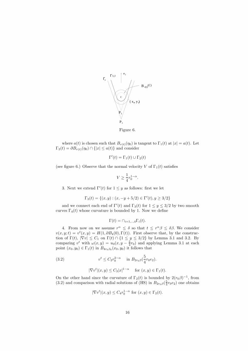
2. In the following proof positive constants Ci’s only depend on θ0. Let ustake (r0β, r0) ∈ Γ0, for 0 < r0 < 1/4. Then there is a ball Br(0)(η0) of radius

r(0) = β√

β2 + 1r0 such that

Br(0)(η0) ∩ Ω(u0) = (±r0β, r0)

(see figure 6.) We construct a free boundary Γ(t) in B2(0)∩ y ≤ 1 as follows:For 0 ≤ t ≤ rα

0 β we consider r(t) = r(0) − 14r1−α

0 t and

Γ1(t) = (x, y) ∈ Γ0 + r(t)e2 : |x| ≥ a(t)

15

C

( x , y )0 0

ΓΓ0

P 0

P t

e2

B r(t)(C)

)( t

Figure 6.

where a(t) is chosen such that Br(t)(η0) is tangent to Γ1(t) at |x| = a(t). LetΓ2(t) = ∂Br(t)(η0) ∩ |x| ≤ a(t) and consider

Γ′(t) = Γ1(t) ∪ Γ2(t)

(see figure 6.) Observe that the normal velocity V of Γ1(t) satisfies

V ≥ 1

4r1−α0 .

3. Next we extend Γ′(t) for 1 ≤ y as follows: first we let

Γ3(t) = (x, y) : (x,−y + 5/2) ∈ Γ′(t), y ≥ 3/2and we connect each end of Γ′(t) and Γ3(t) for 1 ≤ y ≤ 3/2 by two smooth

curves Γ4(t) whose curvature is bounded by 1. Now we define

Γ(t) = ∩i=1,..,4Γi(t).

4. From now on we assume rα ≤ δ so that t ≤ rαβ ≤ δβ. We considerv(x, y; t) = vt(x, y) = H(1, ∂B4(0), Γ(t)). First observe that, by the construc-tion of Γ(t), |∇v| ≤ C1 on Γ(t) ∩ 1 ≤ y ≤ 3/2 by Lemma 3.1 and 3.2. Bycomparing vt with ω(x, y) = u0(x, y − 5

4r0) and applying Lemma 3.1 at eachpoint (x0, y0) ∈ Γ1(t) in B4r0β0

(x0, y0) it follows that

(3.2) vt ≤ C2r2−α0 in B2r0β(

5

4r0e2).

|∇vt|(x, y) ≤ C3|x|1−α for (x, y) ∈ Γ1(t).

On the other hand since the curvature of Γ2(t) is bounded by 2(r0β)−1, from(3.2) and comparison with radial solutions of (HS) in B2r0β( 5

4r0e2) one obtains

|∇vt|(x, y) ≤ C4r1−α0 for (x, y) ∈ Γ2(t).

16

5. From above estimates and by symmetry, there is C5 > 0 such thatv(x, y; t) = v(x, y; C5t) satisfies

vt/|∇v| − |∇v| ≤ C5r′(t) − |∇v| ≤ 0 on Γ(t).

Therefore v is a supersolution of (HS) in B4(0)× (0, C6rα0 β). Now Theorem

2.7(b) yieldsu ≤ v for t ∈ [0, C6r

α0 β].

As a consequence it follows that,

H1(x, rα0 β) ≤ C7r0 for |x| ≤ r0β.

and

H1(r0β, t) ≤ C8(r(t) − r(0)) =C8

4r1−α0 t for 0 ≤ t ≤ rα

0 β.

and we can conclude.

For the lower bound of H1(x, t), a straightforward computation using Lemma3.6 and explicit values of u0 leads to the following estimate:

Lemma 3.9. Let u be as in Lemma 3.8 with π < θ0 < 2π. Then there is aconstant C, δ > 0 independent of θ0 that

H1(x, t) ≥ C min[(t

β)1/α,

|x|1−α

β2−αt].

for 0 ≤ |x|, t ≤ δβ, where β = min(1, β).

Proof of Theorem 1.2(a) with π < θ0 < 2π: It follows from Lemma 3.8and Lemma 3.9.

2

Next we state and prove the n-dimensional version of Theorem 1.2(a). LetΩ be a bounded domain in IRn which satisfies

(3.3) Ω ∩ B3(0) = x = (x′, xn) ∈ IRn : xn ≤ |x′| cotθ0

2.

We further suppose that Ω contains K = B1(−5en), en = (0, .., 1). We define0 < θn < π be the dimensional constant such that with θ0 = θn in (3.3) theharmonic function u0 = H(1, K, Ω) has quadratic decay at x = 0, namely

u0(0,−ren) = O(r2)

for small enough r. We define t(P ),δ(P ) and ζ(P ) as in (1.1)-(1.2). For aviscosity solution u of (HS) with initial data u0, we define H1(x

′, t) = xn(x, t)−xn(x′, 0) where

xn(x′, t) = supxn : (x′, xn) ∈ B1(0) ∩ Γt(u).

We also denote a ' b if the C1a ≤ b ≤ C2a for dimensional, positive constantsC1 and C2.

17

Theorem 3.10. Let u(x, t) be a viscosity solution in IRn×[0,∞) with the initialdata u0 and fixed boundary data 1 and with θn < θ0 < 3π/2. Then u is uniqueand

t(P ) ' δ(P )|P |α−1

where 2−α is the decay rate of u0 at x = 0, namely u0(0,−ren) = O(r2−α)for small r. In particular α → 1 as θ0 approaches π.

Since the proof of Theorem 3.10 is parallel to the case n = 2, we only sketchthe outline of the proof below.

Sketch of the proof for Theorem 3.101. As in the proof of Theorem 1.2(a), we will prove the equivalent statement

in terms of H1(x′, t) for |x′| ≤ 1:

H1(x′, t) ' min[t1/α, t|x|1−α].

First we need to prove the following lemma, which corresponds to Proposi-tion 3.4.

Lemma 3.11. Let u be the minimal supersolution of (HS) with u0, θ0 and thefixed boundary data given as in Theorem 3.10. Then there is a dimensionalconstant C such that

t(P ) ≤ Cδ2(P )

u0(ζ(P ))

for P ∈ B1(0) ∩ (IRn − Ω). In particular t(P ) = 0 if P ∈ Γ0(u) and u is theunique viscosity solution of (HS) with initial data u0.

The last assertion of above lemma follows from Theorem 2.8. For the proofof the lemma we replace the barrier Ψ in the proof of Proposition 3.4 to

Ψ(x, t) =((2 + cnt)/|x|)n−2 − 1

(2 + cnt)n−2 − 1

where cn = 5−n and proceed similarly.

Corollary 3.12. Suppose that u is given as in Lemma 3.11 and let α given asin Theorem 3.10. Then for c > 0 depending only on θ0 and n,

H1(x′, t) ≥ c min[t1/α, t|x|1−α].

The proof of Corollary 3.12 is the same as that of Corollary 3.5.2. It remains to obtain

H1(x′, t) ≤ C min[t1/α, t|x|1−α]

for a dimensional constant C. As in the two-dimensional case we have to con-struct barrier functions separately for the cases θn < θ0 ≤ π and π < θ0 < 3π/2.For the first case we proceed as in the proof of Theorem 1.2(a). The main dif-ference is in the construction of Γ(t) in step 2.(a)-2.(d), defining xn(x, t) in

18

different regions of the form a < |x′| < b instead of defining y(x, t) in differentregions of the form a < |x| < b. For the second case we proceed as in the proofof Lemma 3.8, where the main difference is again in the construction of Γ′(t) interms of replacing the axis e2 by en and (x, y) by (x′, xn).

2.Now we proceed to prove Theorem 1.4. Here we use the self-similar solutions

constructed in [KLV]. For π/2 < θ0 < 2π let us consider U θ0

R : a weak solution(see [KLV] for definition) of (HS) in BR(0)× (0,∞) with initial data UR(z, 0) =r2−α[cos(2 − α)θ]+ and fixed boundary data

Uθ0

R (z, t) = R2−α[cos(2 − α)θ]+ on ∂BR(0).

It was shown in [KLV] that U θ0

R (x, t) is increasing with respect to t and Rand and locally uniformly converges to a continuous function U θ0 in IRn× [0,∞)as R → ∞, where Uθ0(z, t) = t2/α−1f( z

t1/α ) is a continuous self similar solution

of (HS). In fact one can obtain exact formula for U θ0 for π/2 < θ0 < 2π usingconformal mappings (see Appendix in [KLV].)

Proof of Theorem 1.4(a):1. For R > 1 we consider

uR(z, t) := R2−αu(z

R,

t

Rα) in BR(0).

We observe that there is a constant A > 0 such that

(3.4) A := limr→0

u0(z)

(r2−α cos(2 − α)θ)+

Therefore we can choose 0 < δ = δ(R) < A, δ(R) → 0 as R → ∞ which satisfies

A − δ ≤ uR(z, 0)

[r2−α cos(2 − α)θ]+≤ A + δ in Ω0(uR) ∩ BR(0).

Note that uR is a viscosity solution of (HS) in BR(0) × (0, 1).2. First we consider the case π/2 < θ0 < π. Due to Theorem 1.2(a)

d(Γt(u), Γ0(u)) ≤ CR−α for 0 ≤ t ≤ R−α. Hence it follows that for any smallε > 0

(3.5) u∗R(z, 1) ≤ (A + δ)(1 + ε)U θ0+ε

R (z, 0) on ∂BR(0)

if R is sufficiently large. Since U θ0

R ≤ Uθ0 and Uθ0 is increasing in time, byTheorem 2.7

u∗R(z, t) ≤ (A + δ)(1 + ε)U θ0+ε(z, (A + δ)(1 + ε)t) in BR(0) × [0, 1]

and

lim supR→∞ u∗R(z, t) ≤ lim supε,δ→0(A + δ)Uθ0+ε(z, (A + δ)(1 + ε)t)

→ AUθ0(z, At)

19

where the convergence follows from the explicit formula for U θ. In particular

lim supR→∞

u∗R(z, 1) ≤ AUθ0(z, At) for |z|, t ≤ 1.

3. It is shown in [KLV] that for π/2 < θ0 < π there is B > 0, 1 ≤ σ < 2− αsuch that the following estimate holds:

(3.6) Uθ0(z, 1) ≤ [R2−α cos(2 − α)θ + BRσ cos(σθ) + O(1)]+ on ∂BR(0)

It follows that for any small ε we have

(A − δ)(1 − ε)Uθ0−ε(z, (A − δ)(1 − ε)t) ≤ uR(z, t)

if R is sufficiently large. Hence one can argue as in step 1 to yield that

AUθ0(z, At) ≤ lim infR→∞

uR(z, t) in |z|, t ≤ 1.

And thus uR uniformly converges to AU θ0(z, At) in the domain |z|, t ≤ 1. Inparticular, by self-similarity of U θ0 there is C = C(θ0) > 0 such that

limR→∞

uR(0, t) = Ct1/α.

4. For π < θ0 < 2π similar arguments apply. In this case due to Theorem1.2(b)

d(Γt(u), Γ0(u)) ≤ CR−1 for 0 ≤ t ≤ R−α

if R is sufficiently large.For the upper bound of the self-similar solution corresponding to (3.6), one

can use a slight modification of the supersolution constructed in the proof ofLemma 3.8 to yield that

Uθ0(z, 1) ≤ [R2−α cos(2 − α)θ + O(1)]+ on ∂BR(0).

The rest of the proof is parallel to that of step 2-3.2

We next apply reflection arguments to show that the free boundary staysLipschitz in space for small time.

Lemma 3.13. Let u be a viscosity solution of (HS) with the initial data givenin Case A. Then for any small constant 0 < τ < min[θ0, 2π − θ0], there existsδ, ρ > 0 depending on θ0 and τ such that u is monotone increasing along S :=K(θ0 − τ,−e2) in Bρ × [0, δ).

Proof. 1. Let us fix 0 < τ < min[θ0, 2π − θ0] and for each unit vector p whichhas angle θ0 − kτ with −e2, consider

lp = z ∈ IR2 : z · p = 0.To prove the lemma we only have to show that u is monotone increasing alongp ∈ ∂K in Bρ × [0, δ). Let B+

1 be the intersection of B1(0) and one side of lp inthe direction of p. Depending on θ0 we choose k < 1 such that Γ0 is away fromlp (see figure 7a-7c): then there are three cases which requires different analysis.

20

lppl

p

e2

0u > 0

7−c

l p

p

p

7−b

e2 e2

7−a

Figure 7.

(a) For 0 < θ0 ≤ π/2− 32τ , we choose k = 1 so that both legs of Γ0 lies in B+

1 ;

(b) For π/2 + 32τ ≤ θ0 < 2π, we choose k = 1 so that both legs of Γ0 lies in

B1(0) − B+1 ;

(c) For |θ0 − θ0| ≤ 32τ , we choose k = 3/4 so that one leg of the wedge

Γ0 ∩ B1(0) lies in B+1 and the other leg lies in B1 − B+

1 .

2. First let us assume (a). Set ω as the reflection of u with respect to lp.Observe that ω solves (HS) with ω = u on lp. Let us choose δ = δ(τ) such thatω(z, t) = 0 on (∂B1(0) − ∂B+

1 ) for t ∈ [0, δ). Since ω = 0 at t = 0, by Theorem2.7 we obtain

(1 − h)ω∗(z, t − h) ≤ u(z, t) in B+1 × [h, δ)

for any h > 0. Hence by lowersemicontinuity of ω we obtain ω ≤ u in B+1 ×[0, δ).

This implies that u(z, t) is increasing in the direction of p if z ∈ lp ∩B1(0). Thesame argument follows for shifts of lp by small distance ε0 in the ±e2 directionwith a smaller choice of δ > 0. (For shifts towards −e2 direction, the argumentworks since ω ≤ u in B+

1 at t = 0 by comparison principle of harmonic functions.Hence u is increasing along K in the domain

Σ = ∩p∈K ∪ lp + εe2 : |ε| ≤ e0 × [0, δ),

which contains a small cylinder Bρ × [0, δ).3. Next we assume (b). In this case we apply Lemma 3.6 and 3.7. Due

to Lemma 3.6, we may assume that u0(z) is monotone increasing along S inB1 and u is indeed strictly increasing along S in Ω(u) ∩ B1. Moreover for anycompact subset D of Ω0, by the continuity of u in time at t = 0, for any ε > 0there is δ > 0 such that u is ε-monotone along the direction p in D× [0, δ]. Dueto Lemma 3.4 if we choose ε small enough this yields to the full monotonicityof u in the direction of p in D × [0, δ].

Now consider ω defined as in step 1. We compare u and ω in B+1 . Let us

choose a small neighborhood N of Γ0(ω) ∩ ∂B+1 so that ω(z, 0) < u0(z) on N

21

Γ

l p

0

e 2

B 1

N

Figure 8.

(see figure 8 above.) Due to above argument, there is δ > 0 such that

ω ≤ u on (∂B+1 −N ) × [0, δ].

We choose δ small enough such that ω ≤ u on ∂B+1 × [0, δ]. Now ω ≤ u on

the parabolic boundary of B+1 × [0, δ] and the argument follows as in step 2.

to yield that u is monotone increasing in the direction of p in a small cylinderBρ(0) × [0, δ].

4. Finally in the case of (c) combining above two arguments leads to theconclusion. Hence the lemma follows.

2

For the rest of this section we assume the additional hypotheses of Theorem1.4(b): that is, we suppose that Ω0 is starshaped with respect to P0 and Γ0 isC1,1 with respect to P0. Next lemma provides a lower bound for the propagationspeed of the free boundary for θ0 > π/2:

Lemma 3.14. Let u be as in Theorem 1.2(a) with π/2 < θ0 < 2π. Then thereexists A, B > 0 depending on the size of the support of u0 such that

(1 + Aε)u((1 + ε)z, (1 + Aε)2t + Bε) ≥ u∗(z, t) for t > 0.

Proof 1. For π ≤ θ0 < 2π the gradient |∇u0|, formally the initial speedof propagation, is bounded from below on Γ0 and hence it is easy to prove thelemma. The proof is parallel to Lemma 3.4 in [K3].

2. Hence we only consider cases π/2 < θ0 < π. Due to Theorem 2.7 andthe fact that ut ≥ 0, we only have to show that there is A, B > 0 such that

ω(z, t) = (1 + Aε)u((1 + ε)z, (1 + Aε)2t + Bε)

satisfies ω(z, 0) ≥ u0(z) for z ∈ ∂K. Since Γ0 is preserved under dilation inB1(0), due to Theorem 1.2(a) ω(z, 0) > 0 on Γ0 ∩B1(0) for any B > 0. Next wechoose B > 0 such that ω(·, 0) > 0 on Γ0 outside of B1(0). (Such B exists sincethe support of u0 is compact and outside of B1(0) Γ0 is C1,1.) Finally since|∇u|(·, t) is bounded on ∂K we can choose A > 0 such that ω(·, t) ≥ 1 on ∂K.Now the comparison principle for harmonic functions yields the conclusion.

22

2

Remark Heuristically speaking, from Lemma 3.14 one obtains that

ut

|∇u|(z, t) ≥ |z|2At + B

for (z, t) ∈ Γ(u).

Proof of Theorem 1.4(b):Since Ω is starshaped with respect to the origin and since u = 1 on ∂K it

follows that

(3.8) u(z, t) ≥ u∗((1 + ε)z, (1 + ε)t) in Q.

Lemma 3.13 and above inequality with Lemma 3.14 provide the Lipschitzcontinuity of u and Γ(u) for small time 0 ≤ t ≤ δ. Moreover the nondegeneracyof |∇u| on Γ(u) follows from Lemma 3.14 (see [K3] for details.) Now the resultsin [K2] yields the theorem.

2

4 Cusp

Note that Lemma 3.9 gives us a lower bound for the normal distance traveledby the free boundary with constants independent of θ0. We would like to obtainparallel result for the upper bound, so that we can apply these estimates to thecusp (B), that is when the opening of the cone θ0 tends to 2π as we approachthe vertex. Recall that for given π/2 < θ0 < 2π, we define

β0 = π − θ0/2, β = tanβ0 and α = 2 − π/θ0.

In particular β → 0 and α → 3/2 as θ0 → 2π.

Lemma 4.1. Let u be given as in Lemma 3.8 with 3π/2 < θ0 < 2π. Then thereare constants δ, C > 0 independent of θ0 such that for 0 ≤ |x|, t ≤ δβ we have

H1(x, t) ≤ Cmin(t1/α

β1/α,|x|1−α

β2−αt).

Proof 1. Below we construct a supersolution of (HS) for 0 ≤ t ≤ β basedon a free boundary Γ(t) which we construct as follows. Note that α > 1.

(a) For yt ≤ y ≤ 1/2 where yt = ( tβ )1/α · 1

1−β , we define Γ1(t) as follows:

(x±(y, t), y) ∈ Γ1(t) where

x±(y, t) = ±[βy − 1

4

∫ t

0

(y − (s

β)1/α)1−αds].

(b) Next for y ≤ yt we put a circular arc Γ2(t) connecting two points (x±(yt, t), yt)so that the tangent line of Γ2(t) coincides with that of Γ1(t) at y = yt.Let us consider Γ(t) = Γ1(t) ∪ Γ2(t).

23

(c) For y ≥ 1/2 we extend Γ(t) as in the proof of Lemma 3.8 such that Γ(t)has curvature less than 1 in the set 1/2 ≤ y ≤ 1 ∩ B2(0) and Γ(t) issymmetric with respect to axis y = 3/4.

For simplicity let us assume δ = 1. We consider

v(x, y; t) = vt(x, y) = H(1, ∂B4(0), Γ(t)).

We would like to show that v is a supersolution of (HS) for 0 ≤ t ≤ β.2. Normal velocity of Γ(t).(a) By definition the normal velocity of Γ(t) at yt < y ≤ 1 is bigger than

1

2|∂tx

±(y, t)| =1

8(y − yt + ytβ)1−α.

(b) From a straightforward computation it follows that |x±(yt)| = cytβ where1/2 < c < 1 is independent of t and hence |x±(yt)| increases as t increases. Onthe other hand one can verify that at y = yt the tangent line of Γ(t) hasslope Cβα−1, where C is independent of t. Therefore the curvature of Γ2(t) isdecreasing with respect to t and the normal velocity of Γ2(t) attains its minimumat y = yt, which is

limy→yt

[the normal velocity of Γ1(t) at (x±(y, t), y)] ≥ 1

4(ytβ)1−α.

Hence the normal velocity of Γ2(t) is greater than 14 (ytβ)1−α.

3. Estimate of |∇v| on Γ(t)(a) First observe that, since Γ(t) has uniformly bounded curvature in Γ(t)∩

1/4 ≤ y ≤ 1, by Harnack inequality and Lemma 3.1 we obtain |∇v| ≤ C0 inΓ(t) ∩ 1/4 ≤ y ≤ 1. Thus we only have to estimate |∇v| on Γ1(t) ∪ Γ2(t).

(b) Below we denote C as positive constants independent of β. For later usewe compute the curvature κ(y, t) of the free boundary Γ1(t) at(x±, y), x± := x±(y, t). Note that

(y − yt + ytβ) ≤ (y − ys + ysβ) ≤ 2(y − yt + ytβ) for t/2 ≤ s ≤ t.

Therefore

|κ(y, t)| =|x+

yy |

(1+(x+y )2)3/2

≤ C(y − yt + ytβ)−1−αt · (1 + (y − yt + ytβ)−2αt2)−3/2

If (y − yt + ytβ)α ≤ t then

κ(y, t) ≤ C(y − yt + ytβ)−1+2αt−2 ≤ Ct−1/α ≤ Cy−1t β−1/α.

On the other hand if (y − yt + ytβ)α ≥ t then

κ(y, t) ≤ C(y − yt + ytβ)−1−αt ≤ Ct−1/α ≤ Cy−1t β−1/α.

24

Hence we obtain

(4.1) |κ(y, t)| ≤ Cy−1t β−1/α ≤ C(ytβ)−1.

Also note that since x±(yt) = cytβ with 1/2 < c < 1,

(4.2) Γ2(t) has constant curvature κ ≤ 2(ytβ)−1.

For 0 ≤ t ≤ β let us consider

ht(x, y) = h(x, y; t) := u0(x, y − yt) in B1/2.

Then C0 ≤ ht(0,−1/4) ≤ 1 and ht > 0 in Ωt(v) ∩ B2(0). Hence by Lemma 3.2vt ≤ Cht in B1/2. In particular

v(·, t) ≤ C(ytβ)2−α on ∂B2ytβ(0, yt) for 0 ≤ t ≤ β.

(c) We scale

v(x, y; t) = (ytβ)α−2v(ytβx, (ytβ)(y − yt); t)

so that v ≤ C3 on ∂B1. Also from (4.1) and (4.2) the scaled free boundary Γt(v)has bounded curvature in B1(0). These facts and comparison with radiallysymmetric harmonic functions yields that

|∇v(·, t)| ≤ C4(ytβ)1−α on Γ2(t) for 0 ≤ t ≤ β.

(d) It remains to estimate the derivative on Γ1(t). Consider a ball of radiusytβ centered in (x0, y0) ∈ Γ1(t) and v(x, y; t) = v(ytβ(x − x0), ytβ(y − y0); t).Again due to estimates (4.1)-(4.2) the curvature of Γt(v) is bounded independentof β, t. On the other hand Γt(h) is at most ytβ away from Γt(v), and thus

v(1/2, 0; t) ≤ Cht(x0 +1

2ytβ, y0) ≤ C(y0 − yt + ytβ)1−α(ytβ).

Hence by comparison with radially symmetric solutions and applying Lemma3.1, it follows that |∇v(x0, y0; t)| ≤ C(y0 − yt + ytβ)1−α.

4. Above estimates show that vt − C|∇v|2 ≥ 0 for C > 0: independent ofβ for 0 ≤ t ≤ β. Hence v(x, y; t) := v(x, y; Ct) is a supersolution of (HS) inB4(0) × (0, β/C). Moreover u0(x, y) ≤ v(x, y; 0) in B4(0), and hence due toTheorem 2.7

u(x, y; t) ≤ v(x, y; t) in B4(0) × [0, β/C].

In particular it follows that for 0 < r < 1/C

(a) H1(x, rαβ) ≤ Cr for x ≤ rβ;

(b) H1(rβ, t) ≤ C 1β r1−αt for 0 ≤ t ≤ rαβ,

25

1/4

e 2

β

β/2

2β /4( )β,

ΓΓ ( v )0 0

Figure 10.

which leads to the conclusion.2.

Proof of Theorem 1.2(b):1. As before we will prove the equivalent statement

H1(x, t) ' min[t2/5, |x|−3/4t].

The lower bound of H1(x, t) follows from Proposition 3.4 and straightforwardcomputation. Therefore it remains to obtain the upper bound of H1(x, t).

2. For 32π ≤ θ0 < 2π, Consider v0(x, y) : a harmonic function in Ω(v0) with

v0 = 1 on ∂K and

Γ(v0) =

∂W (θ0,−e2) + 14βe2 for x : |x| ≤ β2/4 ∩ B2(P0)

Γ0 otherwise

(see figure 10).Since Ω(u0) ⊂ Ω(v0), u0 ≤ v0. Let v solve (HS) with initial data v0 and

fixed boundary data v = 1 on ∂K. Then u ≤ v and due to Lemma 4.1 there isδ > 0 such that

H1(x, δβα+1) ≤ Cβ for |x| ≤ δβ2.

andH1(δβ

2, t) ≤ Cβ−αt for 0 ≤ t ≤ δβ1+α.

Since 0 < β < 1/2 is arbitrary, we argue as in previous step to obtain

H1(x, t) ≤ C min(t2/5, |x|−3/4t) for |x|, t ≤ δ.

2

5 Touching fingers

Lastly let us suppose that Ω0 is given as in (C). Let us consider u(x, y; t): aviscosity solution of (HS) with initial free boundary Γ0 and fixed boundary data

26

Γ1Γ1

1

xβ β,( )y

βy2

Γ Γ0 0

Figure 12.

1 for (x, y) ∈ ∂K. Then u0 = sup(u10, u

20), where

ui0 = H(1, ∂B1/10((−1)ie1), ∂B1((−1)ie1)).

Thereforeu ≥ sup(u1, u2),

where ui is the solution of (HS) with initial data ui0 and fixed boundary data 1

on ∂B1/10((−1)ie1). In particular, this implies that

(5.1) H1(x, t) ≥ C min[t1/2, |x|−1/2t] for 0 ≤ |x|, t ≤ 1.

On the other hand notice that for any 3π/2 < θ0 < 2π, u0 ≤ vθ0, where

vθ0= H(1, ∂K, Γθ0

) withΓθ0

= ∂Ωθ0,

(5.2) Ωθ0= [W (θ0,−e2) + yβe2] ∩ [W (θ0, e2) − yβe2]

where

yβ = β−1[√

β2 + 1 − 1],1

2β ≤ yβ ≤ β.

Also one can easily verify that

(5.3) Γθ0∩ Γ0 = (xβ , yβ) = (β2 + 1)−1/2(

√

β2 + 1 − 1, β).

(see figure 12.) For later use we state the following lemma:

Lemma 5.1. Let v(x, y) be the harmonic function in IR2 − Γa where

Γa = (0, y) : y ∈ IR − (0, a)

with v = 0 in Γa and v = 1 at (±1, 0). Then v(0, a/2) ≤ 2a.

Proof. Let Ω = IR2 − Γa. Let us consider a conformal mapping ω = zz−ai .

Then ω maps Ω one-to-one to IR2 − (0, y) : y ≥ 0, ∞ to (0, 1), and (±1, 0)to (±1/(1 + a2), a/(1 + a2)). Now we take ζ = ω1/2 in Ω and observe that Ω is

27

mapped one-to-one to IR2− = (x, y) : y < 0, ζ(∞) = (±1, 0) and ζ((±1, 0)) =

P±a , where

P±a = (±(

2 + a2

2 + 2a2)1/2,

a

(2 + 2a2)1/2).

Let δx be the delta function at (x, 0) and let f be a harmonic function in R2−

such that f = c[δ1 + δ−1] on y = 0 for some c > 0 and f = 1 at P±a . Indeed

if we choose c small enough then

f ≤ 4a[−y

(x − 1)2 + y2+

−y

(x + 1)2 + y2]

and hence v = f(ζ) satisfies our hypothesis with

v(0, a/2) = f(√

1/2,−√

1/2) ≤ 2a.

2

Corollary 5.2. Let h(x, y) = H(1, ∂K, Γ2) where Γ2 = ∂[Ωθ0∩ B2(0)]. Then

there is c > 0: independent of θ0 such that, for (x, y) ∈ Γθ0∩ B1(0),

|∇h| ≤

cβα−1|y − yβ |1−α for y − yβ ≤ β/2

c for β/2 ≤ y − yβ ≤ 1.

Proof. 1. Below we denote C as positive constants independent of θ0.Observe that by Lemma 5.1 and by comparison principle h(0, 0) ≤ Cβ. Hencethe first inequality follows by Lemma 3.1 applied in Bβ(0, 0).

2. Next for (x, y) ∈ Γθ0with |y| ≥ β/2 ( we may assume that x ≥ 0,) we

compare h with v = (x − β(y − yβ))+ in D := B2(0) ∩ x ≥ β2 ∩ Ω(v). Sinceh ≤ Cv on ∂B1/10(e1) and on ∂D (due to the previous argument), it followsfrom Lemma 3.1 that h ≤ Cv in D, which yields our assertion.

2.Now we are ready to prove that the inequality (5.1) holds in the other di-

rection as well.Proof of Theorem 1.2(c):

1. Let us choose 2π−θ0 small enough so that 0 < β = β(θ0) < δ, where δ > 0is to be chosen later. For given θ0, we change the coordinates (x, y) → (x, y−yβ)and construct a free boundaryΓ+(t) =

⋃

i=1,2,3 Γi(t) for 0 ≤ t ≤ β2 for 0 < y ≤ 1/2 as follows.

(a) Γ1(t) = (x±(y, t), y) : 2yt ≤ y ≤ 1/2 where yt = t1/2(1 − β)−1 and

x±(y, t) = ±(βy − t).

(b) Γ2(t) = (x±(y, t), y) : yt ≤ y ≤ 2yt where

x±(y, t) = ±[βy − (1 − β)2y2/4−∫ t

(1−β)2y2/4

(β/2)α−1(y − s1/2)1−αds].

Observe that Γ+(t) is C1 at y = 2yt.

28

(c) For y ≤ yt we construct Γ3(t) as a circular arc connecting two endpointsof Γ2(t) at y = yt so that Γ+(t) is C1 at these points.

We define

Γ(t) = Γ+(t) ∪ Γ−(t), Γ−(t) = (x, y) : (x,−y − 2yβ) ∈ Γ+(t).

Lastly we connect Γ(t) and ∂[B2(e1)∪B2(−e1)]∩|y| ≥ 3/4 with straight lines.By barrier arguments with radial solutions one can easily check that the regionΩ(t) with boundary ∂K and Γ(t) includes Ωt(u) − |y| ≤ 1/2 for 0 ≤ t ≤ β2.Consider

v(x, y; t) = vt(x, y) = H(1, ∂K, Γ(t)).

We would like to show that v is a supersolution of (HS) in |y| ≤ 1/2× [0, β2].In particular in the series of computations below we always assume 0 ≤ t ≤ β2.

2. Normal velocity of Γ(t).The normal velocity V of Γi(t) at (x±(y, t), y), i = 1, 2 is greater than

12 |∂t(x

±)(y, t)|, where

|∂t(x±)(y, t)| ≥

1 if (x±, y) ∈ Γ1(t),

(β/2)α−1(y − yt + ytβ)1−α if (x±, y) ∈ Γ2(t).

Next to estimate the normal velocity of Γ3(t), we compute x+(yt, t):

x+(yt, t) = βyt − (1−β)2

4 y2t −

∫ t

t/4(β/2)α−1(yt − s1/2)1−αds

((1 − β)yt = t1/2) = βyt − (1−β)2

4 y2t − cβα−1y3−α

t ,

where 1/4 < c < 1/2 is independent of t. Since 1 < α < 32 and

yt ≤ β/(1 − β) we obtain

1

8βyt ≤ x+(yt, t) ≤ βyt

for 0 < β < 1/10. Moreover x+(yt, t) increases as t increases. Furthermorestraightforward computation as above yields that ∂t(x

+)y(yt, t) > 0 if β is suffi-ciently small. In particular the tangential slope of Γ2(t) at y = yt, (x+

y )−1(yt, t),decreases as time increases. Since x+(yt, t) is increasing with respect to t, thisimplies that the curvature of Γ3(t) is decreasing with respect to time. Hence itfollows that the normal velocity of Γ3(t) attains its minimum at y = yt, whichis

limy→yt

[ the normal velocity of Γ2(t) at (x+(y, t), y)] ≥ 1

2y1−α

t .

Hence it follows that

the normal velocity of Γ3(t) ≥1

2y1−α

t .

29

3. Estimate of |∇v| on Γ(t).(i) As before we compute the curvature κ(y, t) of the free boundary Γ(t) at

(x+(y, t), y), 0 < y ≤ 1/2. First observe that ΓI(t) has curvature zero. Nextobserve that from above estimates we have |(x+)y(y, t)| ≤ β2−α ≤ 1. Hence onΓ2(t) we have(5.4)|κ(y, t)| ≤ 2|(x+)yy(y, t)|

≤ (α − 1)2∫ t

(1−β)2y2/4(β/2)α−1(y − s1/2)−α−1ds

+4βα−1y1−α

(t ≤ (1 − β)2y2) ≤∫ (1−β)2y2

(1−β)2y2/4(β/2)α−1(y − s1/2)−α−1ds + 4βα−1y1−α

(s = (1 − β)2y2γ) ≤ y1−αβα−1∫ 1

1/4(1 − (1 − β)γ1/2)−α−1dγ + 4βα−1y1−α

≤ y1−αβ−1 + 4βα−1y1−α

(yt ≤ y) ≤ 5y−1t β−1

Moreover note that, since |x±(yt, t)| > ytβ/8,

(5.5) Γ3(t) has constant curvature κ ≤ 8(ytβ)−1.

As before we denote C as positive constants independent of β. Next we considerht = H(1, ∂K, Γt(h)) where

Γt(h) = ∂[Ωt ∩ B2]

andΩt = [W (θ0,−e2) + yte2] ∩ [W (θ0, e2) − (yt + 2yβ)e2].

Due to Corollary 5.2 there exists C1 > 0 such that

|∇ht| ≤

C(yt)α−1|y − yt|2−α if |y − yt| ≤ yβ ,

C if |y − yt| ≥ yβ .

Note that d(z, Γt(h)) ≤ ytβ for z ∈ Γ(t) ∩ |y| ≤ 1/2. Now due to estimates(5.4) and (5.5) one can proceed as in the proof of Lemma 4.1 to compare v andht and to deduce that there exists C2 > 0 such that

|∇v(·; t)| ≤

C on Γ1(t);

C(β/2)α−1|y − yt + ytβ|1−α on Γ2(t);

Cβ1−α on Γ3(t).

30

Thus v(x, y; t) = v(x, y; Ct) is a supersolution of (HS) in |y| ≤ 1/2×[0, β2/C2].Since u0 ≤ v(x, y; 0), proceeding as in the proof of Theorem 1.2(a) it followsthat u ≤ v for 0 < t < β2/C. Now we obtain

H1(x, β2/C2) ≤ Cβ for |x| ≤ β2.

Moreover, since (xβ , yβ) ∈ Γ0 (see (5.3)) and yβ ≥ 2yt for 0 ≤ t ≤ β2/4, we canchoose C large enough that

H1(xβ , t) ≤ [the normal velocity of Γ1(t)] ·

t

β≤ Ct/β for 0 ≤ t ≤ β2/C.

Since 0 < β < δ is random with sufficiently small δ and β2/4 ≤ xβ ≤ β2, weobtain that

H1(x, t) ≤ C min(t1/2, |x|−1/2t) for 0 ≤ |x|, t ≤ δ

and thus we can conclude due to above estimate and (5.1).2

References

[ACS] I. Athanasopoulos, L. Caffarelli and S. Salsa, Regularity of thefree boundary in parabolic phase-transition problems, Acta Math.,176(1996), 245-282.

[C1] L. Caffarelli, A Harnack inequality approach to the regularity of freeboundaries, Part II: Flat free boundaries are Lipschitz,Comm. PureAppl. Math., 42(1989), 55-78.

[C2] L. Caffarelli, A Harnack inequality approach to the regularity offree boundaries, Part I: Lipschitz free boundaries are C1,α, Rev. Mat.Iberoamericana 3 (1987), no. 2, 139-162

[D] B.E. Dahlberg, Harmonic functions in Lipschitz domains, Harmonicanalysis in Euclidean spaces, Part 1, pp. 313–322, Proc. Sympos. PureMath., XXXV, Part, Amer. Math. Soc., Providence, R.I., 1979

[H] S.D. Howison, Cusp development in Hele-Shaw flow with a free sur-face,SIAM J. Appl. Math.46 (1986), 20-26.

[K1] I. Kim, Uniqueness and Existence result of Hele-Shaw and Stefan prob-lem, Arch. Rat. Mech. Anal., published online.

[K2] I. Kim, Regularity of free boundary in one phase Hele-Shaw problem,preprint.

[K3] I. Kim, Long time regularity of Hele-Shaw and Stefan problem, preprint.

[KLV] J.R. King, A.A. Lacey and J.L. Vazquez, Persistence of corners in freeboundaries in Hele-Shaw flow, Euro. J. Appl. Math., 6(1995), 455-490.

31