Systems & Control Letters 56 (2007) 122–132www.elsevier.com/locate/sysconle

Asymptotic stability of infinite-dimensional semilinear systems:Application to a nonisothermal reactor

Ilyasse Aksikasa,∗, Joseph J. Winkinb, Denis Dochaina,1

aCESAME, Université catholique de Louvain, 4 Av G. Lemaître, B-1348 Louvain-la-Neuve, BelgiumbDepartment of Mathematics, University of Namur, 8 Rempart de la Vierge, B-5000 Namur, Belgium

Received 17 November 2004; received in revised form 21 July 2006; accepted 25 August 2006Available online 18 October 2006

Abstract

The concept of asymptotic stability is studied for a class of infinite-dimensional semilinear Banach state space (distributed parameter)systems. Asymptotic stability criteria are established, which are based on the concept of strictly m-dissipative operator. These theoretical resultsare applied to a nonisothermal plug flow tubular reactor model, which is described by semilinear partial differential equations, derived frommass and energy balances. In particular it is shown that, under suitable conditions on the model parameters, some equilibrium profiles areasymptotically stable equilibriums of such model.© 2006 Elsevier B.V. All rights reserved.

Keywords: Nonlinear contraction semigroup; Asymptotic stability; Strict m-dissipativity; Nonlinear infinite dimensional systems; Partial differential equation;Nonisothermal plug flow reactor; Tubular chemical reactor

1. Introduction

Stability is one of the most important aspects of system the-ory. The fundamental theory of stability, established by Lya-punov, is extensively developed for finite-dimensional systems.Many results on the asymptotic behavior of nonlinear infinite-dimensional systems are known, for which the dissipativityproperty plays an important role, see e.g. [10,12,6,18,17]. Herewe are interested in the asymptotic stability of a class of infinite-dimensional semi-linear systems which contains tubular reactormodels.

Tubular reactors cover a large class of processes in chemicaland biochemical engineering (see e.g. [13]). They are typicallyreactors in which the medium is not homogeneous (like fixed-bed reactors, packed-bed reactors, fluidized-bed reactors,…)and possibly involve different phases (liquid/solid/gas). Suchsystems are sometimes called “Diffusion–convection–reaction”systems since their dynamical model typically includes thesethree terms. In particular the dynamics of nonisothermal axial

∗ Corresponding author. Tel.: +32 10 47 25 96; fax: +32 10 47 21 80.E-mail address: aksikas@csam.ucl.ac.be (I. Aksikas).

1 Honorary Research Director FNRS.

0167-6911/$ - see front matter © 2006 Elsevier B.V. All rights reserved.doi:10.1016/j.sysconle.2006.08.012

dispersion or plug flow tubular reactors are described by semi-linear partial differential equations (PDEs) derived from massand energy balances.

The objective of this paper is basically twofold. The first goalis to develop a theory concerning the asymptotic stability ofsemilinear distributed parameter systems. The second goal is toapply this theory to a nonisothermal plug flow reactor model.

More specifically, this paper is dedicated to the asymptoticstability of a class of semilinear infinite-dimensional Banachstate space (distributed parameter) systems. This theory is ap-plied to a nonisothermal plug flow tubular reactor model, whichis described by semilinear partial differential equations con-taining nonlinear terms which stem from the Arrhenius law. Inparticular it is shown that, under suitable conditions on the sys-tem parameters, some equilibrium profiles are asymptoticallystable equilibriums of such model. Roughly speaking the mainstability condition is that a Lipschitz constant of the nonlinearpart of the model is sufficiently small with respect to the decayrate of the (exponentially stable) semigroup generated by thelinear part of the model. This stability condition is illustratedby means of some numerical experiments.

In order to make this paper as readable as possible, in partic-ular for non-experts in infinite-dimensional systems, we have

I. Aksikas et al. / Systems & Control Letters 56 (2007) 122–132 123

written it with sufficient details especially concerning the basicconcepts and results of infinite-dimensional system theory.

The paper is organized as follows. Section 2 contains someproperties concerning nonlinear contraction semigroup theory.Notably an asymptotic stability criterion in Banach space isstated, which is based on the concept of strictly m-dissipativeoperator. In Section 3, asymptotic stability criteria are estab-lished for a class of semilinear infinite-dimensional systemsby applying the result stated in the previous section. Section 4deals with an infinite-dimensional state space description of anonisothermal plug flow reactor model. Section 5 is devoted tothe asymptotic stability analysis of this model.

2. Asymptotic stability in Banach space

In order to study the asymptotic stability of semilinearinfinite-dimensional systems, some preliminary concepts andresults are needed, that are related to the theory of nonlinearabstract differential equations on Banach spaces. More specif-ically this section is devoted to some properties of nonlinearcontraction semigroup theory [6,16,19,5,17] and to a paramountknown result related to LaSalle’s invariance principle: seeTheorem 5. In addition the concept of strict m-dissipativity isintroduced, which leads to the stability Theorem 6.

Let us consider a real reflexive Banach space X equippedwith the norm ‖ · ‖. Let D be a nonempty closed subset of X.

Definition 1. A (strongly continuous) nonlinear contractionsemigroup on D is a family of operators �(t) : D → D, t �0,satisfying:

(i) �(t + s) = �(t)�(s) for every s, t �0; �(0) = I .(ii) ‖�(t)x − �(t)x′‖�‖x − x′‖ for every t �0 and every

x, x′ ∈ D.(iii) For every x ∈ D, �(t)x → x as t → 0+.

The infinitesimal generator A� of the nonlinear contractionsemigroup �(t) (on D) is defined on its domain

D(A�) ={x ∈ D : lim

t→0+ t−1[�(t)x − x] exists

}

by

A�x = limt→0+ t−1[�(t)x − x], for every x ∈ D(A�).

Definition 2. Let A be an operator with domain D(A).(i) A is said to be dissipative if, for all x, x′ ∈ D(A) and

for all � > 0,

‖x − x′‖�‖(x − x′) − �(Ax − Ax′)‖,

or equivalently, for all x, x′ ∈ D(A), there exists a boundedlinear functional f on X such that f (x −x′)=‖x −x′‖2 =‖f ‖2

and f (Ax − Ax′)�0.In additionA is said to be strictly dissipative if the conditions

above hold with strict inequalities, for all x, x′ ∈ D(A) suchthat x �= x′.

(ii) A is said to be (strictly) m-dissipative if it is (strictly)dissipative and R(I −A)=X, where R(T ) denotes the rangeof an operator T.

Comment 3. (a) By [17, p. 99], if A is a dissipative operator,then for all � > 0, (I−�A)−1 is well-defined and non-expansiveon R(I − �A), i.e. for all y, y′ ∈ R(I − �A),

‖(I − �A)−1y − (I − �A)−1y′‖�‖y − y′‖.

(b) By [17, Proposition 2.109, p. 100; Corollary 2.120, pp.106–107], if A is a m-dissipative operator, then A is the gen-erator of a unique nonlinear contraction semigroup �(t) onD := D(A). Hence for any x0 ∈ D, the corresponding statetrajectory t �→ x(t, x0) := �(t)x0 ∈ D exists on (0, ∞) and isdifferentiable almost everywhere whenever x0 ∈ D(A) suchthat (d/dt)�(t)x0 = A�(t)x0 for almost all t in (0, ∞) (seee.g. [17, Proposition. 2.98(iii), p. 93]). In other words, for anyx0 ∈ D(A), x(t, x0) := �(t)x0 is the unique solution of thefollowing nonlinear abstract Cauchy problem:{

x(t) = Ax(t), t > 0,

x(0) = x0.(1)

(c) Assuming that A is dissipative, the conclusions of (b) fol-low also from a weaker condition than the m-dissipativity one(see [17, Corollary 2.120]). This condition is given as follows:

conv(D(A)) ⊂⋂�>0

R(I − �A), (2)

where conv(S) denotes the closure of the convex hull of theset S.

Definition 4. Consider the system (1) and assume that A gen-erates a nonlinear contraction semigroup �(t). Consider anequilibrium point x of (1), i.e. x ∈ D(A) and Ax = 0. x is anasymptotically stable equilibrium point of (1) on D if

∀x0 ∈ D, limt→∞ x(t, x0) := lim

t→∞ �(t)x0 = x.

In what follows we also need the following important result(see Theorem 5), which is strongly related to the well-knownLasalle’s invariance principle, see e.g. [17,12]. In order to statethis result, the following concepts and notations are needed. If�(t) is a nonlinear semigroup of contractions on D, for anyx0 ∈ D, the orbit �(x0) through x0 is defined by

�(x0) := {�(t)x0 : t �0},and the �-limit set �(x0) of x0 is the set of all states in Dwhich are the limits at infinity of converging sequences in theorbit through x0, i.e. more specifically x ∈ �(x0) if and onlyif x ∈ D and there exists a sequence tn → ∞ such that

x = limn→∞ �(tn)x0.

Observe that �(x0) is �(t)-invariant, i.e. for all t �0,�(t)�(x0) ⊂ �(x0). Recall that the distance between a point

124 I. Aksikas et al. / Systems & Control Letters 56 (2007) 122–132

x ∈ X and a subset � ⊂ X is given by

d(x, �) := inf{‖x − y‖ : y ∈ �}.Theorem 5 below is a slightly modified version of [12, Theorem3]. The present version can be deduced from [17, Proposition3.60, Theorems 3.61 and 3.65].

Theorem 5. Consider the system{

x(t) = A�x(t), t > 0,

x(0) = x0,(3)

where A� is a dissipative operator such that (2) holds, and let�(t) be the nonlinear contraction semigroup on D = D(A�),generated by A�. Assume that x is an equilibrium point of (3)and (I − �A�)−1 is compact for some � > 0. Then for anyx0 ∈ D, x(t, x0) := �(t)x0 converges, as t → ∞, to �(x0) ⊂{z : ‖z − x‖ = r}, where r �‖x0 − x‖, i.e.

limt→∞ d(x(t, x0), �(x0)) = 0.

It turns out that, under an additional condition, viz. the strictdissipativity of the state operator A�, the �-limit set reducesto the point x, obviously leading to the asymptotic stability ofthe latter.

Theorem 6. Let us consider the system (3) under the assump-tions of Theorem 5. If in addition A� is strictly dissipative,then x(t, x0) → x as t → ∞ i.e. x is an asymptotically stableequilibrium point of (3) on D.

Proof. Without loss of generality assume that x = 0. Considerany x0 ∈ D(A�). By the first paragraph of the proof of [12,Theorem 5, pp. 100, 104], �(x0) ⊂ D(A�). Let us prove that�(x0) = {0}. Consider any x ∈ �(x0) and recall that �(x0) isa �(t)-invariant subset of the sphere {z : ‖z‖ = r}. Hence, forall t �0, �(t)x ∈ �(x0) ⊂ D(A�) and ‖x‖ = ‖�(t)x‖ = r .Observe that, in view of the inclusion

�(x0) ⊂ {z : ‖z‖ = r},it is enough to prove that x =0, i.e. that the sphere {z : ‖z‖=r}reduces to the origin. In order to get a contradiction, assumethat x �= 0. Then,

for almost all t > 0,d

dt�(t)x = A��(t)x. (4)

Moreover, for every h < 0 and every bounded linear functionalf such that

f (�(t)x) = ‖�(t)x‖2 = ‖f ‖2 = r2,

there holds

f (�(t + h)x − �(t)x)�f (�(t + h)x) − f (�(t)x)

�‖f ‖‖�(t + h)x‖ − f (�(t)x)

�r‖�(t + h)x‖ − r‖�(t)x‖�r (‖�(t + h)x‖ − ‖�(t)x‖).

Therefore, one has

d

dt‖�(t)x‖2 = lim

h→0−‖�(t + h)x‖2 − ‖�(t)x‖2

h

= limh→0−

‖�(t + h)x‖ − ‖�(t)x‖h

· (‖�(t + h)x‖ + ‖�(t)x‖)� lim

h→0−f (�(t + h)x − �(t)x)

rh· 2r

�2f (A�(t)x).

Using the strict dissipativity of the operator A�, it follows that

d

dt‖�(t)x‖2 �2f (A��(t)x) < 0 a.e. in (0, ∞). (5)

Therefore, for all t �0, ‖�(t)x‖ < ‖x‖. This contradicts the factthat ‖�(t)x‖ = ‖x‖ = r . Hence

for all x0 ∈ D(A�), �(x0) = {0}. (6)

Now let us consider any x0 ∈ D (not necessarily in D(A�)).Let � > 0 be arbitrarily fixed. By the density of D(A�) in D,there exists y0 ∈ D(A�) such that ‖x0 −y0‖ < �/2. It follows,by the fact that �(t) is a contraction semigroup, that,

for all t �0, ‖x(t, x0) − x(t, y0)‖ <�

2. (7)

Since y0 ∈ D(A�), it follows from (6) that �(y0)={0}, whencethere exists T > 0 such that,

for all t > T , ‖x(t, y0)‖ <�

2. (8)

It follows from (7)–(8) that, for all t > T ,

‖x(t, x0)‖�‖x(t, x0) − x(t, y0)‖ + ‖x(t, y0)‖ < �.

Consequently, 0 is an asymptotically stable equilibrium pointof (3) on D. �

Comment 7. In view of its proof, especially inequality (5),Theorem 6 can also be proved by using LaSalle’s invarianceprinciple (see e.g. [17, Theorem 3.64, p. 161]) instead of Theo-rem 5. Indeed, the function V(x) := ‖x‖2 can be shown to bea Lyapunov function such that the set {x : V(x) = 0} reducesto 0.

3. Asymptotic stability of semilinear systems

Numerous research works are concerned with semilin-ear evolution equations in Banach spaces and applicationto many classes of partial differential equations: see e.g.[18,20,16,21,19,5,1] and many other references. The idea inthis section is to apply Theorems 5 and 6 to a class of semi-linear systems by writing the state operator A� in Eq. (3)as a sum of two operators, one being the generator of an ex-ponentially stable C0-semigroup of linear operators and theother being a continuous Lipschitz nonlinear operator. Somecriteria are given which guarantee the (strict) m-dissipativityof this sum and the compactness of its resolvent operator, and

I. Aksikas et al. / Systems & Control Letters 56 (2007) 122–132 125

therefore the asymptotic stability of the origin: see Theorem 12and Corollary 13.

For this purpose the following preliminary lemma is needed:

Lemma 8. (i) If N is a Lipschitz operator on D ⊂ X, withLipschitz constant lN , then N − lN I is a dissipative operator;whence for all l > lN , N − lI is a strictly dissipative operator.

(ii) If A1 is a m-dissipative operator and A2 is a Lipschitz(strictly) dissipative operator on X, then A1+A2 is a (strictly)m-dissipative operator.

Comment 9. Properties (i) and (ii) are well-known. For (i) seee.g. [18, Lemma 6.1, p. 245] and for (ii) see e.g. [16, Corollary3.8.2].

Let us consider the following class of semilinear systems:{

x(t) = A0x(t) + N0(x(t)),

x(0) = x0 ∈ D(A0) ∩ F,(9)

where the following assumptions hold:(A1) the linear operator A0, defined on its domain D(A0),

is the infinitesimal generator of a C0-semigroup of boundedlinear operators S0(t) on a Banach space X such that

‖S0(t)‖�Me�t ,

for all t �0, for some � < 0 and M �1, i.e. the C0-semigroupS0(t) is exponentially stable (the growth constant of S0(t), de-noted by �0, is negative).

(A2) there exists a positive constant � such that

(I − �A0)−1 is compact. (10)

(A3) N0 is a Lipschitz continuous nonlinear operator definedon a closed subset F of X, with Lipschitz constant l0.

Let us introduce the following notations:

A := A0 + N0 and D := D(A) = D(A0) ∩ F . (11)

First let us assume that the nonlinear operator N0 is definedeverywhere, i.e. F = X (in this case D = X). Before stating astability theorem for this class of systems, the following lemmasare needed.

Lemma 10. Consider a semilinear system described by (9) andsatisfying conditions (A1) and (A3) with M = 1 and F = X.Assume that −�� l0 (respectively, −� > l0). Then the operatorA is m-dissipative (respectively, strictly m-dissipative).

Proof. The idea is to write the operator A as follows:

A = A0 + l0I + N0 − l0I .

By Lemma 8(i), the fact that N0 is a Lipschitz operator im-plies that N0 − l0I is a Lipschitz dissipative operator. On theother hand, since A0 is the generator of a C0-semigroup S0(t)

with ‖S0(t)‖�e�t , the operator A0 + l0I is the generator of aC0-semigroup Sl(t) such that ‖Sl(t)‖�e(�+l0)t (see e.g. [11,Theorem 3.2.1, p. 110]). It follows from the fact that −�� l0

that Sl(t) is a contraction semigroup, whence A0 + l0I is m-dissipative. Consequently by Lemma 8(ii), the operator A ism-dissipative.

In order to show that the operator A is strictly m-dissipativewhen −� > l0, it suffices to write it as A = A0 + lI +N0 − lI , where −�� l > l0, and to observe that the oper-ator N0 − lI is strictly dissipative (see Lemma 8(i)) andA0 + lI is a m-dissipative operator. The conclusion follows byLemma 8(ii). �

Lemma 11. Consider a semilinear system given by (9) andsatisfying conditions (A1)–(A3) with M = 1 and F = X, suchthat −�� l0. Then the operator (I −�A)−1 is compact, where� > 0 is a constant such that (10) holds.

Proof. Let � > 0 be such that (10) holds. In order to prove thecompactness of the operator (I − �A)−1, let us consider anybounded sequence (vn) in X and prove that the sequence (un) :=(I − �A)−1vn, defined in D, has a converging subsequence.

Observe that vn =un −�Aun and consider a bounded linearfunctional f such that f (un) = ‖un‖2 = ‖f ‖2. Then

f (vn) = ‖un‖2 − �f (Aun).

Using the fact that the operator A is dissipative, we have

‖un‖2 �‖un‖2 − �f (Aun) = f (vn)�‖un‖‖vn‖.

It follows that the sequence (un) is bounded. Now consider thesequence (wn) defined by

wn := (I − �A0)un = (I − �A + �N0)un

= vn + �N0(un).

Since N0 is a Lipschitz operator, it follows from the fact that thesequence (un) is bounded, that so is the sequence (N0(un))).Thus, using the boundedness of (vn), one can conclude that(wn) is bounded; whence, by using the compactness of theoperator (I − �A0)

−1, the sequence (un) = ((I − �A0)−1wn)

has a converging subsequence. �

The following theorem follows directly from Lemmas 10and 11, Theorems 5 and 6, and Comment 3(c).

Theorem 12. Consider a semilinear system given by (9) asin Lemma 11 such that −�� l0. Let �(t) be the nonlinearcontraction semigroup on D, generated by A. Assume that x isan equilibrium profile of (9). Then for any x0 ∈ D, x(t, x0) :=�(t)x0 converges, as t → ∞, to �(x0) ⊂ {z : ‖z − x‖ = r},where r �‖x0 − x‖, i.e.

limt→∞ d(x(t, x0), �(x0)) = 0.

If in addition −� > l0, then x(t, x0) → x as t → ∞ i.e. x isan asymptotically stable equilibrium point of (9) on D.

By using a standard argument, viz. the use of an equivalentvector norm on X, Theorem 12 can be extended to the gen-eral case, i.e. M �1. This extension is needed in several appli-cations, especially for axial dispersion tubular reactor models:see [14].

126 I. Aksikas et al. / Systems & Control Letters 56 (2007) 122–132

Corollary 13. Consider a semilinear system described by (9)and satisfying conditions (A1)–(A3), where F =X. Assume that−� > Ml0. Let �(t) be the nonlinear contraction semigroupon D, generated by the operator A (recall that the operatorA and the subset D are given by (11)). Assume that x is anequilibrium profile of (9). Then for any x0 ∈ D,

x(t, x0) := �(t)x0 → x as t → ∞i.e. x is an asymptotically stable equilibrium point of (9) on D.

Proof. Consider the norm given by

|x| := sup{exp(−�t)‖S0(t)x‖ : t �0}which is equivalent to the norm ‖ · ‖ (see e.g. [18, p. 277,21,p. 19]). It follows that the corresponding operator norm of theC0-semigroup generated by A0 satisfies the condition

|S0(t)|�e�t for all t �0.

In addition N0 is a Lipschitz operator relatively to thenorm ‖ · ‖ with Lipschitz constant l0. Hence N0 is also aLipschitz operator with respect to | · |, with Lipschitz con-stant l′0 = l0M . Moreover, −� > l′0. The conclusion follows byTheorem 12. �

Comment 14. It is well-known that, for all � ∈ (�0, 0) (where�0 < 0 denotes the growth constant of the semi-group S0(t)),there exists a constant M� such that

∀t �0, ‖S0(t)‖�M�e�t .

By the proof of [11, Theorem 2.1.6(e)], there exist a time t�and a constant M0,� �1 such that

∀t � t�, ‖S0(t)‖�e�t

and

∀t ∈ [0, t�], ‖S0(t)‖�M0,�.

The constants t�, M0,� and M� are given, respectively, by

t� := inf{��0, ‖S0(t)‖�e�t , ∀t ��},M0,� = sup

t∈[0,t�]‖S0(t)‖, M� = e−�t�M0,�.

Therefore, the condition −� > Ml0 in Corollary 13 can bereplaced by the weaker condition

l0 < sup�0<�<0

(−�M−1� ) := sup

�0<�<0

(−�e�t�

M0,�

).

In the previous stability results, viz. Theorem 12 and Corollary13, it is assumed that N0 is defined everywhere. This conditionis needed in order to guarantee the m-dissipativity of A (seeLemma 8(ii)). However, observe that, in Theorems 5 and 6,m-dissipativity can be replaced by the weaker condition (2).This observation will be crucial in what follows for establishingthe asymptotic stability of the system (9) when the nonlinearoperator N0 is defined on a convex closed subset F ⊂ X. This

extension is needed for the plug flow reactor model treated inSections 4 and 5. This point was overlooked in an earlier analy-sis, leading to erroneous stability conditions for that applicationin [3]. First the following technical concept is introduced:

Definition 15. Let A be a dissipative operator. Let X0 be asubset of X. A is said to be in Q(X0) if D(A) ⊂ X0 andX0 ⊂ R(I − �A) for all � > 0.

Now we are in a position to state the following importantresult, that is useful when the nonlinearity is not defined every-where:

Theorem 16. Let F be a closed convex subset of X. Considera semilinear system given by (9), satisfying conditions (A2)and (A3), and such that A0 is a closed dissipative operatorwhose domain D(A0) is a linear subspace of X. Assume thatA=A0 +N0 is dissipative, the restriction of A0 on D(A0)∩F

is in Q(F) and the condition

lim inf�→0+ �−1d(F, x + �N0(x)) = 0 for x ∈ D := D(A),

holds. Then A is the generator of a contraction semigroup�(t). Assume that x is an equilibrium point of (9). Then forany x0 ∈ D,

limt→∞ d(x(t, x0), �(x0)) = 0,

where x(t, x0)=�(t)x0. If in addition A is strictly dissipative,then �(t)x0 → x as t → ∞, i.e. x is an asymptotically stableequilibrium point of (9) on D.

Proof. First observe that the compactness of (I − �A)−1 fol-lows from conditions (A2), (A3) and the dissipativity of Aas in the proof of Lemma 11. In order to apply Theorem 5,it suffices to prove condition (2). Let us consider the restric-tion of A0 on D(A0) ∩ F . For the sake of simplicity, we keepthe same notation for this restriction. Using the assumptionthat the operator A0 is closed dissipative on D(A0) and theclosedness of F, it is easy to show that A0 is closed dissipa-tive on D(A0) ∩ F . Also since A0 ∈ Q(F) and D(A0) ∩ F ⊂F , then by [16, Theorem 3.8.1] (where X0 = F , A = A0 andB = N0), A = A0 + N0 ∈ Q(F) with D(A) = D(A0) ∩ F .Hence condition (2) holds since D(A0) ∩ F is convex. Fi-nally, asymptotic stability follows from Theorem 6 when A isstrictly dissipative. �

In the sequel, the asymptotic stability theory developed aboveis applied to a nonisothermal plug flow reactor model: see Sec-tion 5. First the PDEs model is described together with its di-mensionless infinite-dimensional state-space description.

4. Nonlinear plug-flow reactor model

4.1. Nonlinear PDE model

The dynamics of tubular reactors are typically described bynonlinear PDEs derived from mass and energy balances. As a

I. Aksikas et al. / Systems & Control Letters 56 (2007) 122–132 127

case study, for the purpose of illustrating the main theoreticalresults derived in Sections 2 and 3, especially Theorem 16, weconsider a nonisothermal plug flow reactor with the followingchemical reaction:

A −→ bB,

where b > 0 denotes the stoichiometric coefficient of the reac-tion. If the kinetics of the above reaction are characterized byfirst order kinetics with respect to the reactant concentrationCA (mol/l) and by an Arrhenius-type dependence with respectto the temperature T (K), the dynamics of the process in such areactor are described by the following energy and mass balancePDEs, where CB (mol/l) denotes the product concentration:

�T

��= − v

�T

�− �H

Cp

k0CA exp

(− E

RT

)

− �0(T − Tc), (12)

�CA

��= −�CA

�− k0CA exp

(− E

RT

), (13)

�CB

��= −v

�CB

�+ bk0CA exp

(− E

RT

), (14)

where �0 := 4h(Cpd)−1 and with the boundary conditionsgiven, for ��0, by

T (0, �) = Tin, CA(0, �) = CA,in, CB(0, �) = 0. (15)

The initial conditions are assumed to be given, for 0��L, by

T (, 0) = T0(), CA(, 0) = CA,0(), CB(, 0) = 0. (16)

In the equations above, v, �H, , Cp, k0, E, R, h, d, Tc, Tinand CA,in hold for the superficial fluid velocity, the heat of re-action, the density, the specific heat, the kinetic constant, theactivation energy, the ideal gas constant, the wall heat transfercoefficient, the reactor diameter, the coolant temperature, theinlet temperature, and the inlet reactant concentration, respec-tively. In addition �, and L denote the time and space inde-pendent variables, and the length of the reactor, respectively.Finally, T0 and CA,0 denote the initial temperature and reactantconcentration profiles, respectively, such that T0(0) = Tin andCA,0(0) = CA,in.

Comment 17. In the particular case T0()=Tin and CA,0()=CA,in for all 0��L, the existence and the invariance proper-ties of the state trajectories of such model on [0, ∞) have beenstudied in [14] (see also the references therein), by using a di-mensionless variable equivalent model. We shall also use sucha model here: see notably Section 4.3.

Observe that in Eqs. (12)–(16), the product concentration CB

is known if the reactant concentration CA and the temperatureT are known. Therefore, we will only consider the two firststate components, viz. the reactor temperature and the reactantconcentration. Their dynamics will be described by means of an

infinite dimensional system description derived from an equiv-alent nonlinear PDE dimensionless model. Such an approach isstandard in tubular reactor analysis (see e.g. [14] and referencestherein) and is briefly developed in the following subsection.

4.2. Infinite dimensional system description

Let us consider two new state variables x1(t) and x2(t), t �0,which are defined via the following state transformation givenby

x1 = T − Tin

Tin, x2 = CA,in − CA

CA,in. (17)

Let us consider also dimensionless time t and space z variablesdefined as follows:

t = �v

L, z =

L.

Then we obtain the following equivalent representation of themodel (12)–(13) (without considering the product concentrationdynamics (14)):

�x1

�t= − �x1

�z− �(x1 − xc)

+ � (1 − x2) exp

(�x1

1 + x1

), (18)

�x2

�t= −�x2

�z+ �(1 − x2) exp

(�x1

1 + x1

), (19)

where xc is the dimensionless coolant temperature

xc = Tc − Tin

Tin

and the dimensionless parameters �, �, , and � are related tothe original parameters as follows:

� = E

RT in, � = k0L

vexp(−�), (20)

� = 4hL

Cp dv, = − �H

Cp

CA,in

Tin. (21)

Comment 18. From a physical point of view, one can observethat for all z ∈ [0, 1], and for all t �0, 0�T (z, t)�Tmax and0�C(z, t)�CA,in or equivalently

−1�x1(z, t)�x1,max := Tmax − Tin

Tin

and

0�x2(z, t)�1,

where the upper bound Tmax could possibly be equal to ∞. Itturns out that the case Tmax <+∞ is the most interesting one inthe stability analysis (see below). Moreover, this case is phys-ically feasible: see [13, Theorem 4.1], which shows that undersome physical assumptions, the temperature and the reactantconcentration are bounded.

128 I. Aksikas et al. / Systems & Control Letters 56 (2007) 122–132

The equivalent state space description of the model (18)–(19)is given by the following semilinear abstract differential equa-tion on the Banach space H := L2(0, 1) × L2(0, 1) (equippedwith the norm ‖(x1, x2)‖ := max(‖x1‖2, ‖x2‖2), where ‖ · ‖2denotes the usual norm on the Hilbert space L2(0, 1)):{

x(t) = Ax(t) + N0(x(t)) + B0xc,

x(0) = x0 ∈ D(A) ∩ F,(22)

where A is the linear (unbounded) operator defined on its do-main

D(A) :={x ∈ H : x is a.c,

dx

dz∈ H and x(0) = 0

}(23)

(where a.c means that the function x is absolutely continuous)by

Ax :=⎡⎣− d

dz− �I 0

0 − d.

dz

⎤⎦

[x1x2

](24)

and the nonlinear operator N is defined on the closed convexsubset

F := {x ∈ H : x1 � − 1 and 0�x2 �1}(where the inequalities hold almost everywhere on [0, 1]) by

N0(x) :=

⎡⎢⎢⎣

� (1 − x2) exp

(�x1

x1 + 1

)

�(1 − x2) exp

(�x1

x1 + 1

)⎤⎥⎥⎦ . (25)

The operator B0 ∈ L(H) is the linear bounded operator definedby

B0 = �

[I

0

]. (26)

5. Plug flow reactor model analysis

5.1. Stability analysis

In this part we are interested in the study of the asymptoticstability of any equilibrium profile, which is a solution of theequilibrium ordinary differential equations corresponding to theplug flow reactor PDEs model (22)–(26).

The local stability of any equilibrium profile with constanttemperature has been studied in [4], where it is shown that theoperator of the linearized system generates an exponentiallystable semigroup. This stability analysis was done in the samespirit than the one developed e.g. in [7,8], [9, Section 2.2],for similar hyperbolic PDE models. Here we are interested inobtaining conditions on the model parameters for the globalstability of such semilinear systems.

In terms of dimensionless variables, let us denote by xe :=(x1,e, x2,e)

T ∈ H and xc,e ∈ L2(0, 1) any equilibrium profile,i.e. any solution of the following equations:

Axe + N0(xe) + B0xc,e = 0.

By setting the coolant temperature xc equal to its equilibriumvalue along the reactor, i.e. by taking xc := xc,e in Eq. (22), theplug flow reactor model described by (22)–(26) can be rewrittenas the following abstract differential equation on the Hilbertspace H:{

x(t) = A0x(t) + N0(x(t)),

x(0) = x0 ∈ D(A0) ∩ F,(27)

where A0 is the affine operator defined on its domain D(A0)=D(A) by A0 := A + � with � := (�xc,e, 0)T.

In order to apply Theorem 16, the following lemmas will beuseful. The first one is straightforward: see e.g. [23, Theorem4.1 and Remark 4.1(ii)].

Lemma 19. Consider the operator A given by (23)–(24). Theoperator A generates an exponentially stable C0-semigroupS(t). Moreover,

for all t �0, ‖S(t)‖�1.

Hence A is m-dissipative and A0 is closed dissipative.

Lemma 20. There exists a positive constant � such that theoperator (I − �A0)

−1 is compact.

Proof. Observe that it suffices to show the compactness of(I − �A)−1. Consider the operator Q� := −(d/dz) − �I de-fined on the domain D(Q�) = {f ∈ L2(0, 1) : f is absolutelycontinuous, df/dz ∈ L2(0, 1) and f (0) = 0}. A straightfor-ward computation reveals that, for any � > 0 and for any g ∈L2(0, 1),

((I − �Q�)−1g)(z) = 1

�exp

(−

(1

�+ �

)z

)

×∫ z

0exp

((1

�+ �

)�

)g(�) d�.

Using this identity, it can be easily shown that (I − �Q�)−1 isa Hilbert–Schmidt operator, whence it is compact. The com-pactness of the operator (I − �A)−1 follows by observing that

(I − �A)−1 = diag[(I − �Q�)−1, (I − �Q0)−1]. �

Comment 21. Another way to show the compactness of (I −�Q�)−1 is to prove that the operator Q−1

� (which can be eas-ily computed) is a Volterra operator and hence it is compact.Consequently the operator

(I − �Q�)−1 = Q−1� (Q−1

� − �I )−1

is compact, since the operator (Q−1� − �I )−1 is bounded.

Lemma 22. The restriction of A on D(A) ∩ F is in Q(F).Moreover, assume that, for all x ∈ F ,

limh→0+ h−1d(F, x + h�) = 0. (28)

Then the restriction of A0 on D(A0) ∩ F is in Q(F).

I. Aksikas et al. / Systems & Control Letters 56 (2007) 122–132 129

Proof. First observe that D(A) ∩ F is dense in F. Indeed, thelatter property follows by the proof of [15, Lemma 4.1] (foraxial dispersion tubular reactors), which can be easily adaptedfor the plug flow reactor case. Indeed, that proof is based on(1) the positivity of eAt , and (2) the eAt -invariance of F (see[14, proof of Theorem 4.1]).

Now let us prove that F ⊂ R(I − �A) for all � > 0. Let� > 0, let y ∈ F , then there exists x = (I − �A)−1y ∈ D(A).Recall that ∀t > 0 eAtF ⊂ F (see [14, p. 10]). One has

(I − �A)−1y = 1

�

(1

�− A

)−1

y = 1

�

∫ ∞

0e−t/�eAty dt .

By straightforward calculation, we can prove that for all y ∈ F ,

1

�

∫ ∞

0e−t/�y dt ∈ F ,

and in particular y = eAty ∈ F . Then F ⊂ R(I − �A) andconsequently the restriction of A on F ∩ D(A) is in Q(F).The second assertion follows directly from the first one andTheorem 3.8.1 in [16]. �

Comment 23. It is easy to see that if xc,e is nonnegative thencondition (28) holds.

Concerning the nonlinear operator, many of its propertieswere established in the framework of the trajectory analysisperformed in an earlier work: see [14, Lemmas 3.1 and 3.2].

Lemma 24. The following properties hold:

(i) The operator N0 is a Lipschitz continuous operator on thesubset F.

(ii) For any x ∈ F , the following identity holds:

limh→0+

1

hd(F, x + hN0(x)) = 0.

In order to guarantee the strict dissipativity of the operatorA0 + N0, we need the following condition:

l0 := max(l1, l2) < �, (29)

where l1 and l2 are given by

l1 = | |k0L

v

[exp

( −E

RT max

)+ 4RT in

Ee2

]if

E

2R�Tmax

= | |k0L

vexp

( −E

RT max

) [1 + ET in

RT 2max

]if

E

2R> Tmax

(30)

and

l2 = k0L

v

[Gm + 4RT in

Ee2

]if

E

2R�Tmax

= k0L

v

[Gm + ET in

RT 2max

exp

( −E

RT max

)]if

E

2R> Tmax,

(31)

where

Gm := max0�T �Tmax

∣∣∣∣exp

(−E

RT

)− 4h

k0Cpd

∣∣∣∣ . (32)

Lemma 25. If condition (29) holds, then the operator A0 +N0is strictly dissipative.

Proof. First observe that the operator A0 + N0 can be alsowritten as Av + Nv where the operator Av is defined on itsdomain D(Av) = D(A0) by

Avx :=⎡⎣− d.

dz− �I 0

0 − d.

dz− �I

⎤⎦ [

x1x2

](33)

and the nonlinear operator Nv is given on the closed subset Fby

Nv(x) =[N1(x)

N2(x)

]:= N0(x) +

[�xc,e�x2

]. (34)

It is easy to see that Av generates a C0-semigroup (eAvt )t �0

such that ‖eAvt‖�e−�t . Now let us prove that Nv is a Lips-chitz operator. For all x := (x1, x2)

T and x′ := (x′1, x

′2)

T in F,

‖Nv(x) − Nv(x′)‖

= max(‖N1(x) − N1(x′)‖, ‖N2(x) − N2(x

′)‖).

Hence a Lipschitz constant l0 of the operator Nv is given byl0 = max(l1, l2) where l1 and l2 are Lipschitz constants of theoperators N1 and N2, respectively.

Observe that, by using the state transformation (17), the op-erator N2 can be rewritten as

N2(x1, x2) = k0L

vCA,inCAG(T ) + �,

where the operator G is defined by

G(T ) := exp

(−E

RT

)− �v

k0L.

It follows that

‖N2(x) − N2(x′)‖ = k0L

vCA,in‖CAG(T ) − C′

AG(T ′)‖

� k0L

vCA,in[Gm‖CA − C′

A‖ + CA,inls‖T − T ′‖],

130 I. Aksikas et al. / Systems & Control Letters 56 (2007) 122–132

where ls is a Lipschitz constant of the function exp(−E/RT )

on [0, Tmax) (see below). Consequently,

‖N2(x) − N2(x′)‖� k0L

v[Gm + lsTin]‖x − x′‖;

whence N2 is a Lipschitz operator on D.Now let us compute ls . Observe that the first derivative of

the function g(s) := exp(−k/s), where k is a positive constant,is bounded on the interval [0, Tmax]. Therefore, the functiong is a Lipschitz continuous function on [0, Tmax]. A Lipschitzconstant of g can be estimated by

ls := sup{g′(s), 0�s�Tmax},

where g′(s)= k/s2 exp(−k/s), for 0 < s�Tmax and g′(0)= 0.The study of the function g′ leads to

ls =

⎧⎪⎨⎪⎩

g′ ( k2

) = 4

ke2 if k�2Tmax,

g′(Tmax) = k

T 2max

exp

(− k

Tmax

)if k > 2Tmax.

When applying this result to the case k = E/R, the constant lsis given by

ls =

⎧⎪⎨⎪⎩

4R

Ee2 if E�2RT max,

E

RT 2max

exp

(− E

RT max

)if E > 2RT max.

It follows that the constant l2 given by (31) is a Lipschitzconstant of N2. By using similar computations, it can be shownthat the constant l1 given by (30) is a Lipschitz constant of N1.Finally, by using Lemma 10, condition (29) implies the strictdissipativity of A0 + N0. �

An important consequence of Lemmas 20, 22, 24 and 25,and Theorem 16, is the following theorem giving a criterion ofasymptotic stability for the plug flow reactor model.

Theorem 26. Consider the system (22)–(25) such that condi-tions (28) and (29) hold. Then the operator A := A0 + N0is the generator of a unique nonlinear contraction semigroup�(t) on F. Moreover, for any x0 ∈ F ,

x(t, x0) := �(t)x0 → xe as t → ∞

i.e. xe is an asymptotically stable equilibrium point of the system(22) on F.

Comment 27. (a) Typically, in most cases, the conditionE > 2RT max is satisfied, since the activation energy E is verylarge. In this case, the asymptotic stability criterion of Theorem26 reads as follows:

k0 exp

(− E

RT max

)K <

4h

Cpd,

Table 1Numerical values of process parameters

Process parameters Symbols Numerical values

Superficial fluid velocity v 0.025 m/s

Length of the reactor L 1 m

Activation energy E 11250 cal/mol

Kinetic constant k0 106 s−1

Heat transfer coefficient 4hCpd

0.2 s−1

Inlet reactant concentration CA,in 0.02 mol/LIdeal gas constant R 1.986 cal/(mol K)

Inlet temperature Tin 340 K�HCp

−4250 K L/mol

where the constant K is defined as the maximum of the twofollowing quantities:

| |[

1 + ET in

RT 2max

]and

[Gm exp

(E

RT max

)+ ET in

RT 2max

].

From a physical point of view, the condition above meansthat the heat transfer coefficient must be large enough inorder to dominate a weighted value of the kinetic constantk0 exp(−E/RT max).

(b) On the basis of the (local) stability results obtained e.g.in [4] or [7, p. 18], the stability condition (28), although naturalfrom a theoretical point of view, could possibly appear to beconservative for the specific case studied here. However, thisis how far one can get by using such theoretical tools. Thisspecific point could be an interesting topic for further research,by using possibly classical PDE techniques like the methods ofcharacteristics.

Yet, the theoretical results obtained in Sections 2 and 3 areinteresting on their own and they could also be applied e.g. toaxial dispersion tubular reactor models as well.

5.2. Numerical simulations

In this section, we are interested in numerical simulationsof the open-loop controlled plug flow reactor model (12)–(16).The latter model can be approximated by several methods. Herewe use the finite forward difference method. The parametervalues used here are given in Table 1.

It is theoretically shown in the previous section that, un-der suitable conditions on the system parameters and on thecoolant temperature at the equilibrium, an equilibrium profileis asymptotically stable for the plug flow reactor model. Theequilibrium profile considered here corresponds to a constantcoolant temperature profile. The choice of such equilibriumprofile is motivated by the fact that it is optimal in view tominimize the reactant concentration at the reactor outlet andthe difference between the coolant temperature and the ambienttemperature [22]. Moreover, this equilibrium profile satisfiescondition (28) for a coolant temperature larger than the inlet

I. Aksikas et al. / Systems & Control Letters 56 (2007) 122–132 131

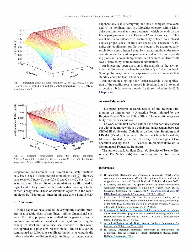
Fig. 1. Temperature using the initial conditions T0(z) = Tin cos(0.2 ∗ z) andCA,0(z) = CA,in cos(0.1 ∗ z) and the coolant temperature Tc,e = 340 K asopen-loop control.

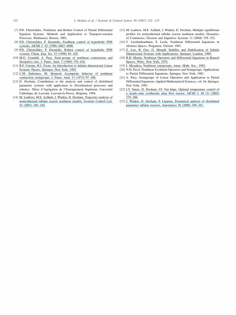
Fig. 2. Reactant concentration using the initial conditionsT0(z) = Tin cos(0.2 ∗ z) and CA,0(z) = CA,in cos(0.1 ∗ z) and the coolanttemperature Tc,e = 340 K as open-loop control.

temperature (see Comment 23). Several initial state functionshave been tested in the numerical simulations (see [2]). Here wehave selected T0(z)=Tin cos(0.2∗z) and CA,0=Cin cos(0.1∗z)

as initial state. The results of the simulations are illustrated inFigs. 1 and 2: they show that the system state converges to thechosen steady state. These observations agree with the resultpredicted by Theorem 26, since in this case l0 =14 and �=20.

6. Conclusion

In this paper we have studied the asymptotic stability prop-erty of a specific class of semilinear infinite-dimensional sys-tems. First this property was studied for a general class ofnonlinear infinite-dimensional state space systems by using theconcept of strict m-dissipativity: see Theorem 6. This resultwas applied to a plug flow reactor model. The results can besummarized as follows. A semilinear model is asymptoticallystable under the conditions that (a) its linear part generates an

exponentially stable semigroup and has a compact resolvent,and (b) its nonlinear part is a Lipschitz operator with a Lips-chitz constant less than some parameter, which depends on thelinear part parameters: see Theorem 12 and Corollary 13. Thisresult has been extended to nonlinearity defined on a closedconvex proper subset of the state space: see Theorem 16. Fi-nally, any equilibrium profile was shown to be asymptoticallystable for a nonisothermal plug flow reactor model under someconditions on the system parameters and on the correspond-ing (constant) coolant temperature: see Theorem 26. This resultwas illustrated by some numerical simulations.

An interesting open question is the analysis of the asymp-totic stability property when the condition l0 < � does not hold.Some preliminary numerical experiments seem to indicate thatstability could be lost in that case.

Another interesting topic for further research is the applica-tion of the stability results proved in Sections 2 and 3, to axialdispersion tubular reactor models like those studied in [14,15,7,Chapter 4].

Acknowledgements

This paper presents research results of the Belgian Pro-gramme on Interuniversity Attraction Poles, initiated by theBelgian Federal Science Policy Office. The scientific responsi-bility rests with its authors.

The work of the first named author has been partially carriedout within the framework of a collaboration agreement betweenCESAME (Université Catholique de Louvain, Belgium) andLINMA (Faculty of Sciences, Université Chouaib Doukkali,Morocco), funded by the State Secretary for Development Co-operation and by the CIUF (Conseil Interuniversitaire de laCommunauté Française, Belgium).

The authors thank Pr. Hans Zwart (University of Twente, En-schede, The Netherlands) for stimulating and helpful discus-sions.

References

[1] B. Abouzaïd, Régulation des systèmes á paramètres répartis aveccontraintes sur la commande. Mémoire du Diplôme d’Etudes SupérieuresAppprofondies, Université Chouaib Doukkali, El Jadida, Morocco, 2003.

[2] I. Aksikas, Analysis and LQ-optimal control of infinite-dimensionalsemilinear systems: application to a plug flow reactor, Ph.D. Thesis,Université Catholique de Louvain, 2005. http://edoc.bib.ucl.ac.be:81/ETD-db/collection/available/BelnUcetd-11302005-154241/

[3] I. Aksikas, J. Winkin, D. Dochain, Asymptotic stability of anonisothermal plug flow reactor infinite-dimensional model, Proceedingsof the Sixth IFAC Symposium on Nonlinear Control Systems, NOLCOS2004, vol. 3, Stuttgart, Germany, pp. 1049–1054.

[4] I. Aksikas, J. Winkin, D. Dochain, Stability analysis of an infinite-dimensional linearized plug flow reactor model, Proceedings of the 43rdIEEE Conference on Decision and Control, CDC 2004, Atlantis, ParadiseIsland, Bahamas, pp. 2417–2422.

[5] A. Belleni-Morante, A. Mc Bride, Applied Nonlinear Semigroups: AnIntroduction, Wiley, New York, 1998.

[6] H. Brezis, Opérateurs maximaux monotones et semi-groupes decontractions dans les espaces de Hilbert, Mathematics Studies, North-Holland, Amsterdam, 1973.

132 I. Aksikas et al. / Systems & Control Letters 56 (2007) 122–132

[7] P.D. Christofides, Nonlinear and Robust Control of Partial DifferentialEquation Systems: Methods and Application to Transport-reactionProcesses, Birkhauser, Boston, 2001.

[8] P.D. Christofides, P. Daoutidis, Feedback control of hyperbolic PDEsystems, AIChE J. 42 (1996) 6063–6086.

[9] P.D. Christofides, P. Daoutidis, Robust control of hyperbolic PDEsystems, Chem. Eng. Sci. 53 (1998) 85–105.

[10] M.G. Crandall, A. Pazy, Semi-groups of nonlinear contractions anddissipative sets, J. Funct. Anal. 3 (1969) 376–418.

[11] R.F. Curtain, H.J. Zwart, An Introduction to Infinite-dimensional LinearSystems Theory, Springer, New York, 1995.

[12] C.M. Dafermos, M. Slemrod, Asymptotic behavior of nonlinearcontraction semigroups, J. Funct. Anal. 13 (1973) 97–106.

[13] D. Dochain, Contribution to the analysis and control of distributedparameter systems with application to (bio)chemical processes androbotics, Thèse d’Agrégation de l’Enseignement Supérieur, UniversitéCatholique de Louvain, Louvain-la-Neuve, Belgium, 1994.

[14] M. Laabissi, M.E. Achhab, J. Winkin, D. Dochain, Trajectory analysis ofnonisothermal tubular reactor nonlinear models, Systems Control Lett.42 (2001) 169–184.

[15] M. Laabissi, M.E. Achhab, J. Winkin, D. Dochain, Multiple equilibriumprofiles for nonisothermal tubular reactor nonlinear models, Dynamicsof Continuous, Discrete and Impulsive Systems 11 (2004) 339–352.

[16] V. Lasshmikantham, S. Leela, Nonlinear Differential Equations inAbstract Spaces, Pergamon, Oxford, 1981.

[17] Z. Luo, B. Guo, O. Morgül, Stability and Stabilization of InfiniteDimensional Systems with Applications, Springer, London, 1999.

[18] R.H. Martin, Nonlinear Operators and Differential Equations in BanachSpaces, Wiley, New York, 1976.

[19] I. Miyadera, Nonlinear semigroups, Amer. Math. Soc., 1992.[20] N.H. Pavel, Nonlinear Evolution Operators and Semigroups: Applications

to Partial Differential Equations, Springer, New York, 1981.[21] A. Pazy, Semigroups of Linear Operators and Application to Partial

Differential Equations, Applied Mathematical Sciences, vol. 44, Springer,New York, 1983.

[22] I.Y. Smets, D. Dochain, J.F. Van Impe, Optimal temperature control ofa steady-state exothermic plug flow reactor, AIChE J. 48 (2) (2002)279–286.

[23] J. Winkin, D. Dochain, P. Ligarius, Dynamical analysis of distributedparameter tubular reactors, Automatica 36 (2000) 349–361.