REDUCTION OF BACKSCATTERING FROM THE INFINITE (NINE ...
162
REDUCTION OF BACKSCATTERING FROM THE INFINITE (NINE AND THE SPHERE BY IMPEDANIIE LOADING Thesis for the Degree of Ph. D. MICHIGAN STATE UNIVERSITY CARL KENNETH DUDLEY 1967
-
Upload
khangminh22 -
Category
Documents
-
view
0 -
download
0
Transcript of REDUCTION OF BACKSCATTERING FROM THE INFINITE (NINE ...

REDUCTION OF BACKSCATTERING FROM
THE INFINITE (NINE AND THE
SPHERE BY IMPEDANIIE LOADING
Thesis for the Degree of Ph. D.
MICHIGAN STATE UNIVERSITY
CARL KENNETH DUDLEY
1967

IHtiSlS
mums.
' T" 117"::
id‘s 7 n
“5533- "_”"”'""~“Y"
‘0
i
This is to certify that the
thesis entitled
REDUCTION OF BA CKSCA TTERING FROM
THE INFINITE CONE AND THE
SPHERE BY IMPEDANCE LOADING
presented by
CARL KENNETH DUDLEY
has been accepted towards fulfillment
of the requirements for
_.Eh._D.._ degree in Electrical Engine ering
//</v\ ’flfkf/Z\
Major professor
Date—MY 19. 1967
0-169


ABSTRACT
REDUCTION OF BACKSCATTERING FROM THE INFINITE
CONE AND THE SPHERE BY IMPEDANCE LOADING
by Carl Kenneth Dudley
The theoretical study on the reduction of the backscattering of
the infinite cone and the sphere by the impedance loading method is
presented. An infinite cone is assumed to be illuminated bya plane
wave at the nose-on incidence. The backscattering of the cone is
minimized by loading the cone surface with (I) a circumferential slot
backed by an impedance, (2) a radial slot backed by an impedance and
(3) a patch impedance. The sphere is given a similar treatment with
the impedance area being in the shape of the wedge and the patch. For
both the infinite cone and the sphere, it is shown that the optimum
impedance for each case can be found to make the backscattering
vanish.

REDUCTION OF BACKSCATTERING FROM THE INFINITE
CONE AND THE SPHERE BY IMPEDANCE LOADING
BY
Carl Kenneth Dudley
A THESIS
Submitted to
Michigan State University
in partial fulfillment of the requirements
for the degree of
DOCTOR OF PHILOSOPHY
Department of Electrical Engineering
1967

M5 ,.,
g/w
ACKNOWLEDGMENT
The author wishes to express his indebtedness to his committee
chairman Dr. K. M. Chen for his guidance and encourgement in the
preparation of this thesis. He also wishes to thank Mr. J. W. Hoffman
of the Division of Engineering Research for the support in the form of
graduate fellowships during the conduct of this research. Appreciation
is also expressed to other committee members: Dr. J. A. Strelzoff,
Dr. David Moursund, Dr. R. J. Reid, Dr. Yilmaz Tokad, and Dr.
Von Tersch.
Finally, grateful acknowledgment is given to Divine Providence
for facilities, both mental and material, making possible the preparation
for and completion of the academic degree which this work culminates.
ii

TA BLE OF CONTENTS
Acknowledgment
List of Figures
Introduction
II.
III.
Scattering from a Perfectly Conducting Unaltered
Cone Surface
1.1. Spherical. Mode Function
1. 2. Boundary Conditions
1. 3. Determination of the Expansion Coefficients
l. 4. Total Field Components
Radiation from an Aperture on a Conducting Cone
2.1. Procedure
2. 2. Boundary Conditions
2. 3. Lorentz Reciprocity Theorem
2. 4. Evaluation of the Unknown Coefficients,
Region I
2 5. The T.M. Modes, Even Terms
2 6. Application of Orthogonality to the Sum
Z. 7. Remaining Coefficients
2 8. The TE Modes
2 9. Determination of Expansion Coefficients,
Region II
2. 10. Scalar Potential. Due to the, Point Sou rce
2.11. The Non~lnfinitesinial Active Source
2.12. Field C(')]Ilp0'“ui."i"_'3 Due to a Specified Electric
Field Intens‘i y in an. Aperture on a Cone
Scattering from a. Cone with a Circmnferential
Slot Inipedan-:;e
3.1. Combination of Previous Results
3. Z. The Cir :umf‘erentiai Slot as an Active Area
3. 3. Surface Current due to the Active Slot
3. 4. The Distant F;eld on the Cone Axis
3. 5. Cancellation of the Distant Fields
3. 6. Circumferential Slot [Impedance
iii
Page
ii
HOWUO
15
15
15
17
22
22
26
31
36
37
39
39
41
44
44
46
47
49
50
52

TABLE OF CONTENTS (concluded)
IV. Scattering from a Cone with a Radial Slot Impedance
4.1. The Radial Slot Source
4. 2. The Surface Currents
4. 3. The Radial Slot Impedance
4. 4. The Finite Radial Slot Impedance
V. Patch Impedance
5.1. The IsotrOpic Impedance
5. 2. Polarity Rotation by Impedance Loading
5. 3. Complete Cancellation using Symmetric
Impedances
5. 4. Generalization and Conclusions
VI. The Fields of the Illuminated Unloaded Sphere
6.1. The Incident Field
6. 2. The Scattered Field
6. 3. The Backseatte red Field
6. 4. The Surface. Current
VII. The Fields Radiated fr'oin an Aperture on the Sphere
7.1. The Expansion Coefficients
7. 2. The Surface Currents and the Radiation Field
VIII. The Wedge linpcdairre on the Sphere
8.1. The Shape of the hnpedance Area
8. 2. Location- of the Wedge. Impedance
IX. The Patch ln'ipedange on. the Sphere
References
Appendix I. Spherical Mode Functions
Appendix II. Properties of the Associated Legendre Functions
iv
Page
56
56
59
6O
62
64
64
74
75
79
82
83
88
93
94
95
95
99
105
105
106
120
121
134

Figure
LIST OF FIGURES
A Loaded Cone Illuminated by a Plane Wave
A Conducting Unaitered Cone Illuminated by a
Plane Wave
A Point Generator on the Cone Surface
A Cone with a Circumferential Slot
A Cone witha Longitudinal Slot
A Cone with a Finite Slot
A Cone with a Patch Impedance
The Unloaded Sphere as a Scatterer.
Page
18
45
57
63
65
84

INTRODUCTION
Interest is being shown lately in the reduction of Radar back—
scattering of metallic objects. The sphere and the cylinder have
already been analyzed.
In this work the infinite cone and some further aspects of the
sphere are investigated and in each case an expression is found
for various impedances which will eliminate the backscattering
from the structure. Both the circmnferential and longitudinal slot
are used separately and other forms of impedances are also dealt with.
A loaded cone such as shown in Figure 1 is illuminated by a
plane wave normal to the axis of the cone. The surface of the cone is
considered as an ideal conductor except for an area in which an imped-
ance is placed. The presence of the impedance causes the radar echo
to be zero in the direction from which the incident wave is coming.
In the method used here the problem is divided into parts. In
the first part the cone is illuminated with no impedance in its surface
and both the surface current IS and the scattered field ES are noted.
Then in the second part the cone is considered without illumination but
with the area in which the impedance is to be placed having a specified
arbitrary field E0. Again the surface current I and the radiation
R
field ER are noted as functions of E0. Next the field E0 is specified
in such a way as to make ER = - E3 in the direction from which the
incident wave is coming. Finally the two situations are combined
using the super position principle to give the desired condition of zero
back scattering. The value of the impedance is the ratio of the field
E0 in the area of the impedance to the total surface current there.

2
The impedance thus found may have to be active. It has the
expression
z=——.—— (1)
An advantage of this method is that it incorporates existing
solutions as parts of the overall problem.
E
incident
plane
wave'CEI
impedance
Figure l. A loaded cone illuminated by a plane wave.

CHAPTER I
SCATTERING FROM A PERFECTLY CONDUCTING
UNALTERED CONE SURFACE
1.1. Spherical Mode Functions
Consider first the illumination of a cone surface without the
impedance. The incident wave is a plane wave traveling in the nega-
tive z direction with the electric field in the y 1- 2 plane. The cone
surface is at an angle 60 from the z axis. The geometry of the prob-
lem is shown in Figure 2. A surface current Isis induced and a
scattered field E5 is produced. The cone is a coordinate surface of
the Spherical coordinate system so the spherical mode functions are
used (see equations (35) in Appendix I).
1. 2. Boundary Conditions
In the equations (35) of Appendix I the constants Amy’ Bmv’
v' are all zero except for m = 1. This is seen by theC ., and D
mV m
geometry of the problem.
Also the only radial functions used are the spherical Bessel
functionsjv and jv' since the region includes the origin where nu, hul.
and hV2 are singular. The boundary conditions on the surface of
the cone which is considered an ideal conductor are
E = E = 0 (2)
Equation (2) applies to the total of both the incident and reflected
parts of the electric field intensity.
Examination of equations (35) of Appendix I,specifica11y the
equations for Er and E
<P

s catte red wave
ml
ml
5 e
x
Figu re 2.
ml
m
incident
plane wave
surface
current
A conducting unaltered cone illuminated
by a plane wave.
I
S

F1 M Z Eli't—U zV(kr) Pin (cos 9) [Amy cos mcb + Bml/ sin mi]
F] n
4’ 2 2—3—r sin6 dr [r21] 13311:,qu sin m‘l’ - Bmv cos 1114):]
m
. d m .+Jw11 V, -é- PU, Cmv' cos m¢+ Dmv' sm met
m
shows that equation (2) is satisfied if
.21-l
P (cos 90) _ d9 pV} koseo)=:0 (3)
Equations (3) determine the eigenvalues V.l and V'i which are
a countable set and may be ordered v0, 1! and V'O, v'I, V2300. la
U'Z, . . . respectively.
With these changes equations (35) become
0° Vi(v.l+l) 1
E :2 ————— ' P [Aicos¢+Bisin¢:]
r r JV. V.i=0 1 I.
Q)
l d . d l '- .
E6 -2 ? d_r [rJuja-é- PV. A.l cos¢ + Bi Sincb]
i=0 ‘ l 1 ‘
Q)
+ ° #2 —-———l ' 12>l c '¢ D 4»J“ sine Jun uh iS‘n ‘ icos,
i=0 1 1
CD
E -2 —i—- A ' P1 A '¢ B 034)cl)- rsine dr rJVi 1x.l 181r1 ' ic
i=0

CD
Vil(I/'i+1) 1 -
Hr:2 r JV'. Pl”. "Cicoscb +DiSln¢:l
i=0 1 ‘
m
1 d . d 1 .
He —; ? d? [1'31”] d_9 pv'. [Ci cos¢ + D.1 Sing-l
i=0 i 1
mm
-' Z '1 ' P1 Asin¢—Bcos¢“06 sine Jvi V.l i i
i=0
b
(1)
_ -1 d . 1 .
Pip-Z m a? [flux] P“. icismi’ “Dim”
i=0
a)
-jw6 Z jv. (1% PU]. [Aicoscb +Bisindj]
. 1i=0
1
(4)
1. 3. Determination of the Expansion Coefficients
The expansion coefficients Bi and Ci must be found using the
condition that as r becomes very large the total field approaches the
incident field. This condition is actually only true for sharp cones.
For example if the cone angle 80 approaches 900 the cone becomes
an infinite sheet the field of which is a standing wave everywhere.
This problem is eliminated later however and need not be a matter
of concern here.
The fact that the incident wave is oriented with the electric
field intensity in the y - 2 plane and that the remainder of the geometry
is independent of 4) indicates that in the x - 2 plane the radial com-
ponent of electric field intensity is zero, and in the y - 2 plane the

7
radial component of magnetic field intensity is zero. Examination of
equations (4) reveals that this can be true only if A.l 2 Di = O.
The scalar functions II and II* for the total field from equations
(25) and (34) in Appendix I are
l l
(D
. 1 .II = Z BiJv. (kr)Pv. (cose)sm¢
i=0
(5)m
II = E C.j , (kr) P ,1 (cose)cos¢
, 1 V1 ”1i=0
The incident electric field intensity is expressed by the equation
E1 = J“? (6)
In spherical coordinates the radial components of electric and
magnetic field intensities from equation (6) are
eJerOS 9 sin9 sincb
Ir
(7)
H __ Yejkrcose
Ir sine cos d)
where Y = V—
In order to find the expansion coefficients B.l and C.l the
orthogonality prOperty of PV1 (cos 9) and -%- Pu,1 (cos 6) in the
i i
interval (0, 80) are used. (See Appendix II, equation (37) ).
Using equations (5) the radial components of the total field
are found to be

co
V.l (Vi+1) 1
Er = 2 Bi r JV. PU. 51nd)1:0 1 l.
(8)
00- v{ (v!l + 1) 1
Hr = 2 C1 r JV, PV' cos¢
i-O ‘ i
For very large r the radial components of the total field as
expressed by equation (8) approach the radial components of the in-
cident field as expressed by Equation (7).
Equating the right-hand sides of equations (7) and (8) and
multiplication by Pul sine or Pv'l sine and integrating over
i i
9 = O to 9 = 90 for large r yields
60
S elkr COS 9 sinZG Pvl (cos 6)d6
O i
60
'= l—l/(V.+1)Bj (kr)S P1(cose) 2 sine d9r i 1 i ll.l 0 Vi
(9)
9.. o _
NAG-S elkr C088 sinZG P ,1(cos€i)d9u U.
o l
9v'i (11'.1 + l) 0 l 2
'= Cijv, (kr)5 [ii-3V, (cose)] sine d6
r i o i
The dots above the equal signs in equations (9) indicate that
the relations are only approximate. On the left-hand side is the
expression for the incident field for large r, while on the right-hand

9
side is the expression for the total field for large r. This approxima-
tion may be improved upon by using the asymptotic forms for jv and
recognizing which part is the incident field and which part is the
reflected field. Equating only the incident parts will eliminate the
problem referred to previously which occurs for cone angles 90 not
greater than 90°.
For large r the asymptotic form for jv 18
l
Jy(kr)-* '-'-cos<kr--V+1 1r)
kr 2
(1'0) ‘
kr >> v
In another form relation (10) is
. v+1 . v+l
3'1, an)» 31;; EN" '7") + e'J‘kr " 2 ‘0]
(11)
kr>>v
The integrals on the left—hand sides of equations (9) can be evaluated
by the method of stationary phase and the results are given here as
6o
. V1011 + 1) .
S; eJkr COS 6 sinZG P121(cos 9) de-_ +———2—— eJkr
(jkr)
r -> 00 (12)
J? 60 'kr os 9 Z l f Vin}.1+1) 'k_ J c . _ J rp 5‘ e Sin 9 P1”. (cos 9) d6_ + —-l-—-l-Z- e
o l (jkr)

10
When equations (12) are combined with equations (9) and
replacing jv with its asymptotic form the result is
vi+1 Vi“
ejkr -1 1 Jim” 2") ‘jikr‘T‘l(jkr)2 = 'F 1 Zkr e + e
9
° 1 2S [PU (cosG)] sine d9 ,
o i
(13)
v'i+1 vi”
6 ejkr ._l 1 j<kr- 2 1r) -j(kr- 2 1r)
“’1? (jkr)2 Z '5 Ci Zkr 8 +8
9
o
.S [pl/'1 (cosefl2 sine d9
0 i
Reducing equations (13) gives
Vi+l Vi“
areJkr ._ Bi eJkr 8‘3 2 7‘ +8 jkr +1 2 T’
k "‘2‘
e
O 15‘ PV (c059) sine d6
0 i
V'i-tl V'l+l
F—S. Jkr .__(_3_i_ eJkr e'J 2 ‘T + Jkr +3 21T
' 'u k ‘ 2
e
r->00 (l4)

11
Here in equations (14) the incident parts are identified by
observing the terms with r dependence. The left-hand side is a
function of eJkr and is strictly due to the incident wave. The
bracket on the right contains two terms eJkr, which compares with
the left-hand side and therefore is due to the incident part, and
-jkr . .e which is due to the reflected part.
Equating only the incident parts of equations (14) gives an
accurate statement in the limit as r —> 00. Thus the expansion
coefficients Bi and C.1 are found.
. TT
_2eJ(Vl+l)E
B. =l 90
l 2 .
k Pu (cos 9) Sin 6 d9
i
(15)
. I 1
-2 J? 8“" 1+” 2c. = “
1 e
0 1 2k 3‘ [PI], (cos 9)] sin 9 d6
0 i
l. 4. Total Field Components
It can be shown that
9o m 2 sineO dPLI?‘ (c059) de/n(coseo). _ l
5 [PM (cos 6)] Sine d8 _ - 21/.“ d6 Y dV
0 1 l 6 v.o l
9 m0 ' 9 8
S Pm (cos ml ZsinGdG-Sm ° Pm(cose) p"(cos 9) 9-912'. J ‘ Zv'.+1 v'. 0 ‘ _ o
O 1 l i 3961/ U-V'
i
(16)

In equation (15) m = 1.
definitions will be given for the following constants.
will be used throughout the remainder of this work.
mi
Ul
mi
VI
mi
WI
mi
12
f:
p
2v,+1
l
md PU (cos 90)
dV :1
ZU'.+1
l
i
2
8 Pin (cos 6)
8661/
9:9
0
v=v'.
l
yin/1+1)
I I
v .1(v .1 + l)
U .mi
d m .[5-9- PV. (cose)] em 90
l9
0
UI
mi
an(cose )sinG
l/ o oi
In order to facilitate the notation, new
These definitions
(17)

13
With substitutions from equations (16) and (17) equations (15)
bec ome
j(v.l+l)%
B. = 2e Wli/ k
The total field components can now be found using these
coefficients in equations (4). The total field components for the
illuminated infinite cone are
°° j(1/ +1) ‘T-2 sin i 3 . 1
Er = ___1_(_}_‘_i_>_ Viwli e JV (kr) Pl! (C089)
:0 i 1
co . 17. .+l)—
_ -2 51nd) . J(V1 2 d .
Ee - kr sin 2 31"" W118 :1"; I‘ll/.0“)i=0 ‘
- I‘lT
d 1 3V2. 1d?)- Pyi (cose ) + kr Wli e l _)V,i(kr)PVIi (cos 6)
dr [rjui(kr)] PVI. (cos 9)
- kr sin 6 Wli e 1 jv'. (kr) 3%- Pwl. (cos 6)
1 1

(D
1)ZY cos 3(v' + .
Hr - kr 4) V' W'll e JV. (kr) P l(cosG)
1:0
CD . 1T
v'.+l)—_ ZY coscb . , J( 1 2 _d__ .
He ‘ kr sine ““9 W11 8 dr rJu'iikr)
i=0
(1 1 jUi'TZLJ.
- 3-6- PV‘. (c039) +kr W1.1 e Vi(kr) PVI (C059)
1 V1.
‘ '. 1) 1ZY Sln “V 1+ 2 d . 1
H4) = - krTing iio W1 e _dr rJV,i(kr) Pu, (cos 9)
i
1r
. , if. __d_ 1+ kr sme W 1.1 e JV-l (kr) d9 PUi (cos 9)
(18)
For the distant field components with r -> 00 the asymptotic
form may be substituted for jV(kr) and hV(Z) (kr) as follows.
jv(kr) —> 1:1; COS (kr _.£/_+;_J;T_>
r +00 (10)
. W
3W“) 2 e-jkr
kr
(2)hi! (kr)-* e

CHAPTER II
RADIATION FROM AN APERTURE ON A
CONDUCTING CONE
2. 1. Procedure
In this chapter the field equations due to a specified electric
field intensity over an arbitrary portion of the surface of a conduct-—
ing cone are sought.
To begin with a point generator is assumed which occupies
no area and lies on the surface of the cone. After the fields due to
the point generator are found they are used as differential elements
of the fields due to the active aperture area and integration yields
the fields due to the entire aperture. The point generator E0 is
located at (r', 90, 42') and consists of components tangential to the
cone surface.
09
2. 2. Boundary Conditions
The cone is considered as an ideal conductor and thus the
homogeneous boundary conditions still apply, and require that except
I l
for(r, 60, (i3)
EZE =0 ate-:9
0
To represent the fields due to this point generator both TM
and TE modes are used. The scalar potentials from equations (25)
and (34) in Appendix I are
15

.-.w
fiv-
Lb
.C
.5»
.C
.7.‘.
.4-

16
II = Z Z 21/ (kr) PV (cos 9) [Amy cos m¢ + Bmv Sin m¢]
m U
(19)
m
II”:< = 2 E zv'(kr)P1/' (c039) [me cos m4) + Dmv.sin m¢]
mv'
As in the case of the illuminated cone the boundary conditions
on the surface of the cone again require that
H O
mPui (cos 90)
(20)
md Pv'i (cos GO)
d9
Thus if m = 1 Vi and v'.1 are defined the same as in Chapter I.
In Appendix II it is shown that v.1, i = O, l, 2, . . . are a different set
for each m. For this reason there should be two subscripts on v as
Vmi when the boundary conditions (20) are used. The m subscript
will be dropped however for the sake of simpler notation. When
these V.l are to be found it must be known to which m they belong.
In the case considered in this chapter there is no incident
field and therefore the radiation condition is satisfied. That is, for
large r the outgoing wave approaches a spherical wave with no radial
component and the r dependence becomes

l7
e-Jkr
kr
r—>CD
2. 3. Lorentz Reciprocity Theorem
The exterior of the cone is divided into two regions as shown
in Figure 3
Region I : r
(21)
Region II : r > r
In statement (21) above ro is assumed less than r'. Since
the origin is in region I the radial function zv(kr) is replaced with
jv(kr) and in region 11 the radiation condition requires the use of
(2)by (kr).
The expansion coefficients will be different in each region.
Region I is bounded by surfaces S and S1 and region II isO
bounded by 80’ S and Sm, the infinite sphere.2!
Now the Lorentz reciprocity theorem is applied to region
II which is
S (FilXfiz) . as: g (EZXfil) . d5 (22)
s s -
In equation (22) the integral is over the entire bounding surface, and
dB is an element of that surface in the outward normal direction.
S=SO+S +Sco (23)
2

11
Figure 3.
18
// \\\
\
\
\
\
\
/\
\__...._\ co
//’ \\ \
/ \ \
/ \ \/ \
\ \
/ \/ {‘0 \ S /\
I 1 0° ‘
’ i Ii ' I
\ I '
\ I I’
\ /
\ S1 / I
) / ,\
\ /«\ S /
----- o /
/
S2 /
/
/
/
/
/
\ "
/ point
generator
(r'. 90. iv)
A point generator on the cone surface.

19
Equation (22) with (23) becomes six integrals
5 (E'IXEZ) . (-9) dSO + S (EX—fig). (8) dSZ
50 S2
II
(I)
3
ml
N
X ml
p—a T :>
a.
U)
o
_ _ A
+5 (E1 X H2). (r) dSm
sco o
._ __ /\ _ _ /\
+5. (EZXH1)- (e) (is.2 + 5‘ (EZX H1)- (r) d5“,
52 Sco
(24)
Performing the triple products in equation (24) yields
.. I ..
5; (E14) H29 E19H2¢) (5180 + is ‘EloHZr Eerth) dsz
o 2
+5; (EIGHZd) ' E1¢H29) dsoo = 8; (E2¢H19 ' E26H1¢)dSO
co 0
+5; (EZCler - EZrHl¢) dSZ + SSUEZGHlCi’ - E2¢H19) dSoo
2 oo
(25)
At this point the fields E1 and E1 are considered to be the
actual fields due to the point generator while E2 and .1712 are the fields
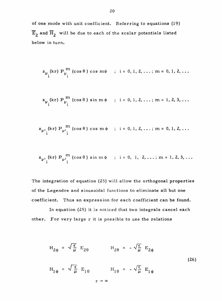
20
of one mode with unit coefficient. Referring to equations (19)
E2 and fiz will be due to each of the scalar potentials listed
below in turn.
zvi(kr)PVr:1(cose)cosm¢ ;i=0,l,2,...;m=0,1,2,...
zvi(kr)PVrin(cose)sinm¢ ;i=0,l,2,...;m=l,2,3,...
zU,i(kr)Pl/,Iin(cose)cosm¢ ; i=0,l,2,...;m=0,1,2,...
zv,i(kr) Py,r:1(cose)sinm¢ ;1=0, 1, 2,...;m= 1,2,3,...
The integration of equation (25) will allow the orthogonal properties
of the Legendre and sinusoidal functions to eliminate all but one
coefficient. Thus an eXpression for each coefficient can be found.
In equation (25) it is noticed that two integrals cancel each
other. For very large r it is possible to use the relations
G 6
H24) = J; E29 H29 = -~/L—_ E24)
(26)
H =J—EE
14> tIm
19 16 14>

21
The integrals over the S30 surface become equal when equations
(26) are used and they are dropped, leaving
SS (E19324) - E1¢H29) dsO -55 (Ezechb - 1324,1119) dSO = K
o o
(27)
where K is defined as
K = 5; (E1¢H2r " Eer2¢) dsz -Ss (EchHir ' EZrchb) dsz
2 2
(28)
Because of the manner in which V.l and V'.l were chosen
E2r = E2¢ = O on surface 52 making the second integral in equation
(28) zero. For the same reason E and E are zero over all of
Ir 14>
S2 except at the point generator where they are EOr and EO¢ which
will be expressed as a Dirac delta function. The eigenvalues 11.1
and V'i were chosen to make the tangential components of electric
field intensity zero on the cone surface but a discontinuity exists
in the scalar pbtentials at the point generator making it possible
for the integrals to be non-zero. The value of K may be found by
integrating only over the source point since the integrand is zero
elsewhere on 52. Thus equation (28) becomes
K = — y (Eer2ct- E1¢H2r) r sin Gd¢dr (29)
source

22
2. 4. Evaluation of the Unknown Coefficients, Region I
Equation (27) will be used to evaluate the expansion coef-
ficients. It is convenient to break this equation into parts, defining
K1, K2, K3, and K4 as follows.
K = SS E19H2¢dSO
0
K2 : BS5 E1 cpHZGdSO
O
(30)
K3 = -5 E29H1¢dSO
50
K4 =S‘ E2¢H19dSO
S0
Thus equation (27) becomes
K=K1+KZ+K3+K4 (31)
The components of E1 and El are expressed in the most
general terms and are taken from equations (35) in Appendix I with
the radial function jV(kr) replacing zv(kr).
2. 5. The TM Modes, Even Terms
In order to find each coefficient E and I? are considered
2 2
to be due to one mode having unit coefficient. For example to

23
find a particular A '1 the scalar potentialsII and II* are chosen
m
as
H : hv (2) (kr) PVmi (cose) cos m'¢
I I
(32)
11* = 0
Using equations (32) in equations (33) in Appendix I gives the
components of E2 and fig as follows.
V I
E2 =—-£ h (2)(kr)Prn (cose)cos m'd)I‘ r V V
I I
_ l :1. , (2) 51 m' .E29 - r dr [r hvl (kr)] d9 [PI/1 (cose):l cos m d)
1 d (2) 1 m' .._ _ 1__ __ 1
E24) - m r dr [r hug (kr)] sine Pvt (cosG) 3mm 4)
H2r —_- O
. 2 l m' .
H.29 = - Jwe m' hV1( ) (kr)-S—.J1—e— PVI (cose) Sin m' d)
. 2 d m'
H24) 2 - Jwe hV£( )(kr) €5- [PI/1 (c058)] cos m' <1)
(33)
In the manner just described equations (30) become

24
[20 -j(.)€rO hVZO-a—()(kr)r[rj v]
1:1}! Vi1‘
0
d m d m' . - u. d1 [Pu Jde [PV1]31n6 [Amicos m¢+BmisinmJ cos m d)
2 2 (2) - m d m.+ w [16er by! (kro) Juli(kro) pV'i (T6- [pl/1]
. _ , 6[Cmism m4) Dmi cos m¢] cos m ct d dd)
60 (D 00
K2 = 5;) 5;) 2:0 :0 -jw€mm' ro 3%[rjvi] by?) (kro)
m: 1: I'
o
1 m m' , . '
. sine Pu, Pu [Ami sm m¢ - Bmi cos m] Sin m (b
2 i 2 ° (Z) _31_ m m'-w Hem rO 312' (kro) hv (kro) [p ] p
I
1 1 d9 ”1
° [C .cosm¢+D ,sinm] sinm'?d9d¢
m1 .m1

25
211' 90 °° °°
K =§S Y Z m-c-i-[rh (21 —d-[r :l
3 A dr v1 dr 32»
0 0m-.-o 1:0 r0 ‘ re
d m' m . 1
as [Pvt] Pv'. [Cmi 5‘“ mt ' Dmi C°S mi] “’3 m 4°
. _<_i_ <2) - - _d_ m' .4. ‘ m+ 3006 r0 dr [r hvl J Jvi (kro) Sine d9 [pl/1]d9 [Pvi]
' rO
. l ,[Ami cos m4) + Bmi Sin m¢J cos m 4) d6 d4)
d (2) . l m' m' ——
+Jw€ m mro dr [r111]! ] Jvi(kro) m Pu! Pvt
r
O
. _ . ,
[Ami Sin m4) Bmi cos m ] Sin m 4) d9 dd)
(34)

26
2. 6. Application of Orthogonality to the Sum
In equations (34) the orthogonal properties of the sine and
cosine functions eliminate all the coefficients except Am'i and
m'i ; i = 0, 1, 2, . . . and the orthogonal property of the Legendre
functions (see Appendix II) eliminate all the Dm'i (m' if 0) and all
is eliminated by thethe A except A If m' = 0 then Dm m m'i '1' '1,
fact that in equations (34) each term containing Dmi has a factor
either m or m'.
With these changes equations (34) become
_ . (2) __d_ .
Kl — -Jw€ Am'l r0 hV (kro) dr r12}!
1ro
2
90( Zn
d m' 9 . 2 ,35 PV (cos ) Sine d9 cos m4) d¢
O f O
. 2 (2) d ._ _ 1 _
K2 - Jwe Am'f m rO by! (kro) dr [:rJVIJ
rO
9 2w
0 1 m' 2 2
SO sine PV (cosG) d9 5 sin m'¢d¢
I O

5;)0 [(3% (P521.(cose))]z sinGdG 5;) c032 m'cbdq;
(35)
In equations (35) the quantities
Zn 211'
5 sin2 m'cbd (b and S cosz m' 4) d¢> (36)
O 0
may be replaced by their equivalent values 1r (1 - 60m.) and
1r (1 + 6 ') respectively where 6 , is the Krondecker deltaom om
I if m'=0
l
on“ 0 if Irv/o
Upon examination of the equations (3 5) it is seen that there is
2 .
a factor m' where ever the quantity

28
211'
. 2 .
5 Sin m'cb dcb is found.
0
This makes it possible to use 11 (1 + 60m) for both the integrals (36)
since for each value of m'
m'211(1- a )0m
lI 3. :1
C + O!
0 3"
Thus equations (35) may be totaled and simplified to give
- - - _d_ (2)K - Jw 6 Am'f 11(1+ 60m,) r031}! (kro) dr [r by! :l
9 m' 2
- rO hviz) (kro) fil} jug] 5‘0 [3% (P121 (Cos 6))]
I
m' P31 (cos 9)
+[ I 1 sin e de (37)sin 9
The bracket which contains the r dependence of equation (37) may be
expressed as

. d (2) (Z) dr JV (krO)-d—r[r hv ] r hv (kr ) d [r JV]
1 1 r O 1 O r 1 r
O O
_. Z _d_ (2) (Z) .9. .
_ ro [JVI (k ) dr (by!) hvl (kr) dr(JV1):, _
r—ro
_ 2 . (2) _ _j_ .
-10 WiJv,’ by! ) - -1, (38)
r
0
where W(jv . 1112(2)) is the Wronskian of the functions jv and
2 1 1 1h < )
1’1
The integral of equation (37) can be reduced as follows (see
equation (46) in Appendix II).
o 2 V
d m' 1 .5;) 3-9- [Pl/1 (cos 9g + sin 9 Sin 9 d9
90 2
m'
= V S [P (cos 9)] sin 9 d 9
1 0 ”1
=(39)
With the substitutions indicated in equations (38) and (39) equation
(3 7) becomes

3O
K=A Y1r(1+5
m‘f(4O)
) _._._._.___.
0m, Wm’f
It is convenient to abbreviate equation (40) by defining constants
N a s
Vim
v.
N 2 11(1 + a )‘W—l‘“ (41)
With the use of definition (41) the coefficients Ami are found to be
KY2ml um
I
This coefficient is for region I defined by relation (21) as
r5 r0 and represents the even term of the TM mode part of the
field set up by the point generator. This can be seen fr01n the fact
that His an even function of (i) and it produces no r component of
magnetic field intensity (see equations (32.) and (33) ).
To evaluate K the same set of fields defined by equations
(33) should be used, and since in these equations Iin = O the K
becomes
K = S - 11qu E11. Silled¢ dr
SOUI‘CG
At this point it becomes clear that the 4) component of the B field
of the point generator does not maintain a TM mode field.

31
The source point is located at (r' , 90, 41' ) and if the Dirac
delta function for E11. is defined as
E 6(r-r'>6(¢-¢'>OI‘
Elr:
rsinG
o
and H2¢ is taken from equations (33), then K becomes
r sin 6
source0
K = X 3'1.) EEor 5(r-r') MiG-4N) (bl/(.12) (led-die [PI/rycos Bile
cos m¢ r sin 9 d¢dr (42)
When the integration in equation (42) is carried out the result is
K = jwe Eor hv(.2) (kr') 21%- [Pi/I: (cos 9 )1 9 cos m¢' (43)
l
The final expression for Ami for region I is found by using equations
(43) and (41).
jk Eor Umi hf) (kr') cos m 4»
A I. = l (44)
The definitions for U , , V. and W , were given in
m1 1 m1
definitions (17), Section 1.4.
2. 7. Remaining Coefficients
The procedure for finding the remaining coefficients is
precisely the same as it was for A _ and it is not necessary to show
m1

32
all the steps involved for each of the other three coefficients. For
comparison purposes the four resulting expressions for K are shown
as follows
_. 2 . (2)
KA ._ Jwe Ami n(1+6om)ro W (JV, hv. )
m1 1 1 r
o
m 2 m 2
—— + —.——— sine d9
0 d9 Sine
K =°w€B-r W(' h(2))B . J 'l'nlTr 0 Jv.’ V.m1 1 1 r
o
m 2 m 2
590 [d Pyi] m Pvi]
- ——-— + . sine d6
0 d9 5m 9
K -uuc 11(l+6 )r W(' 11(2)C - — J ml 0 0 Jv!’ VI )1.
m1 1 1 o
m 2 m 2
90 d PW. m Pu,-
5 —Jé-l-— + —S_i.n—Gl— sinG d9
0
. 2 . (2)
KD .- -le~1Dm-lw rO W (3V1, hu'. )1.
m1 1 1 o
m 2 m 2
60 [(1 Put] mPV,.:]
1 1 . 6 d95 Td + fisin Sin
/
(45)

33
If may be observed that in equations (45) the factor
(1 + 6 ) is not in the equations for K and K . The reasonom B . D .
m1 m1
for this is that B . and D . need not be defined for m = 0 since in
m1 m1
the expressions for the field components, equations (35) Appendix
I, each of these coefficients are multiplied by either m or sin mcb
and both of these are zero when m = 0. However for the sake of
uniformity in the equations the factor (1 + 60m) will be included. This
will not change the values of the coefficients for m = 0 but will give
the convenient relations
KA . KB .
m1 _ m1
I _ B .
m1 m1
Kc . KD .m1 _ m1
I — D 0
m1 m1
It is also seen in equations (45) that the first two equations as a
pair are similar in form to the last two. If in the last two the )1
factors were replaced with (~6) and 11'.l with V.l , then the forms
would be the same. This change in V.l would not affect the values
of
(2)
V'. )W(j,,. .h
i 1
but it does change the values of the integrals. The values of the
integrals of equations (45) can be shown to be

9 dP mP
5:) T + m Sinede
eo
: V. (V.+1) S [Pm(cosG):l sine d9
1 l V.
0 1
Vi
= W“. ‘47)m1
2 2
6 dP, mPl0 Vi U.l
S [—de 1 + i: sin a] swede0
ll
’1‘
A
‘5.
+ )—a
6o m 2
S [P, (coseq sinGdGV.
1
= W. (48)
Because of the similarity between the first two equations
in (45) it is possible to make them into a single combined expression.
If the pair A . and B . are designated as
mi 1111

35
where the "e" and the "0” indicate that the coefficient is associated
with the cos m s and sin m cl) which are even and odd functions
respectively, then the expression for the scalar potential II from
equation (25) in Appendix 1 becomes
00 CD
I I m cos m¢
II : z 2 Amig JV.(kr) PU. (c059) sin m¢ (49)
m: 0 i: O l l
where
\
jk E U h (2) (kr') “’3 mi"
1 or mi Vi sin m¢‘Amie :: (50)
0 (1 + 6 )v. sin eom l O
In equation (50) the bracket
cos nicb'
sin mct’
is due to the fact that the integral over the source point corresponding
to equation (42) becomes
(3)K = 8‘ 31116 E 6(r-r')6(<i>~¢')h (kr)
Amie ' or v.1
0 source
"I cos med m
. d5 [FL'. (1,036)] sin me d¢dr
l 9: 90
(51)

36
2. 8. The TE Modes
If C . and D . are treated in a similar manner as A . and
m1 m1 m1
Bmi were they will be combined as one expression
Cmi= (3 ie
I m1O
D .m1
and the resulting expression for KC is found by combining the
' em1 0
last two equations of (45) to give
V'._ 1
KC -e — Cmie Y "(1+ 60m) W' . (52)m1 0 0 mi
The constants K are also found by integrating over the
-em1O
source point as indicated by equation (29)
K = 5‘ (E14) H2r - Eer2¢) r em 60 d (l) d r (29)
source
point
It was found while working with KA that equation (29) was
mi e0
reduced by the fact that if H’r’ : 0 then H2r = 0. Here however, both
components HZr and Hch are present and integration of equation (29)
gives two parts.

1 i cos m¢'
sin m¢'
d 2 m
Eor m d? [r hV'(. )(kr):|r' PV'. (COS 90) . 1+ 1 1 sin m4)
r' sin 90 -cos m¢'
(53)
This implies that both 4) and r components of the E field of the
point generator contribute to maintain a TE mode of wave.
Equating the right hand sides of equations (52) and (53) and
. I .solv1ng for Cmig gives
d 2Eor m Y U'mi 3-; [r hv,( ) (kr):l
C I = i r' sin m¢
e
0 r' sinZG V'. 11(1 + 6 ) cos m4)
0 1 om
(Z)I _ I
EO¢YU in“ (kr)1 cos mci)
r'sine 11(l+6 ) 5m m4)
0 om
(54)
2. 9. Determination of Expansion Coefficients, Region II
The expressions for the expansion coefficients for region I
are now found, and next the expressions for the coefficients for region
II are to be sought. Before they are, however, it will be convenient
to let the value of r0 become equal to r' making the point source on the
boundary of the two regions. Since r0 does not appear in the expression
for the coefficients they will be unaffected.

38
In order to determine the coefficients for region II it is only
necessary to apply the condition of continuity of the scalar potentials
at the boundary between the two regions. This condition is stated as
r = r' (55)
The only way in which condition (55) can be fulfilled for all
values of 9 and cl) is to make the coefficients satisfy the conditions
A is j (kr') = A H.e 11(2) (kr')m1 V. mio V.
o 1 1
(56)
I , _ II (2) ,
Cmig JV'. (kr) Cmig hV‘i (kr )
1
. . II II . .Solv1ng equations (56) for A 1e and C .e and substitutmg for
mio mio
A .18 and C Ie from equations (50) and (54) gives the expressions
mio mio
. . ,
3k Eor Umi JV.(kr) cos mcp'
II _ 1 (57)
mie _ . sin m¢'o 11 (l + 6 ) V. Sine
om 1 o
. d (2)i I .—
11 EormYU miJZ/iiikr )dr [r hull (kr):l r‘ sin m¢‘
Cmig 2 (1+5 )v' '29 111(2) (k ') 11'11 om .1 Sin 0 r Vii _ r -cos m
E ' YU' .j, (kr')
+ och m1 v i cos mci)‘ (58)
11(1 +6 )r'SLnG sinmd)‘om o

39
2.10. Scalar Potentials Due to the Point Source
Substitution of equations (50), (54), (57), and (58) into equation
(25) and (34) in Appendix 1 for 11 and 11 gives
pym (cos 9)cos m(¢>- ¢')
1
. . (2)co 3k E0 U (kr<)hvi (kr>)
r m1 V.
11:: Z ‘
m=0i: 0 11 (1+ 60m) V.l Sin Go
(5 9)
, d (2) . (2)co EormYU mi a-r- [r hwi (kr):|r' Jy,i(kr<) hwi (kr>)
a)
“* "" 2: ' 2 (2)m: 11 (1 +60m) V'.l sin 90 r' hV'. (kr')
l
Pym (cos 9) sin m (<1) - ¢’)
1
E09) YU'mijV'.l(kr<) huff) (kr>) PVI'I: (C05 6) C03 m (9) ' 9')
11(1+6 )r'sinG
om o
(60)
In equations (59) and (60) the notations r< and r> have been
introduced which are defined as follows. The quantity r< is the lesser
of the two quantities r and r' while r> is the greater of the two.
2.11. The Non-Infinitesimal Active Source
With the finding of the connpleted expressions for H and III<
the field components due to a point generator at (r' , Go , (b') may be
found from equations (33) in Appendix I. If however, instead of a
point source the fields are due to a specified electric field intensity

40
over an arbitrary area on the surface of the cone, then the II" and II
of equations (59) and (60) are used as differential elements of the total
scalar potential and integration yields the total fields. If the field over
the active area is expressed as
§O(r'¢‘) = Eor(r'¢’) ?+EO¢(r'. «111$
'<
then the final expression for the total scalar potentials II}. and II are
as follows.
m* 00 00 mY U'mi Pvt (cos 9)
' 11(1+6 )V'.sin9m: _ om 1 o
Eor(r', cb')sinm(¢' - (Mag-,- [r'héfihkrfl] hug.) (kr> )jv,i(kr<)dr'd¢'
l
.
- i i .12;
Active . (kr')V.
Area 1
co co Y U'ml PVT,n (cos 9)
+ Z 2 ‘m=O i:0 “(1 + 60m)
0
' \ (2)
55 E (r'.¢')cosm(¢'-¢lJ 1(kr h 1 (k1‘ )dr'dCb'
Active O¢ Vi <I Vi >
Area

m: 0 l: O (l + 6 ) V
I I ' (2) I I I
'4) )cosm(<l> 4)) Juikr<lhu (kr>) 1‘ dr (349
Source 1 l (62)
2.12. Field Components due to a Specified Electric Field Intensity
in an Aperture on a Cone.
(cos 9)
Er(r.9. 4»): 11:0 :01 ‘ S) E0r1r'.¢')cosm(¢'-¢1
(1 + 50In)r Source
. . (2) g, .,
r'JV (kr<) hV (kr>) d1 dcp
i i
das cc; Jk Umi -d_9- I: Pu:n (cos 9)]
Ee(r’e’¢) = Z 2 11(1 + s )r V
m=01= 0 0m 1
~0ij .<t>') sm{<b s) I—d- = (k )h(2)(k ) d 'dcb'CO r dr rJU,‘ r< V. r> r
Source 1 l
m U' rpvfn (cos 9) (kr<) h(2,)(kr> )
' J 1 v.
m1 i 5 V i i+
' ' i 5 hi2) (kr‘)51n9s1n9 V.
o
- [Eor(r', (if) m cos m (43‘ - (b) 3%;- (ryht/(IZ) (kr'))
- V'1E0¢(r', ¢') sin m (cb' - (1)) sin 90 h(2,) (kr' ):| d!" (349'
1

42
co co mU .sin9 Pm(cos 9)
6 <1) - Z Z jk ml 0 v.E¢(r, ’ " 11(1 + 6 )r sin 9'sin 9‘ v.
m: 0 .1: O em 0 1
' X S Eor(r' , ¢')sinm(¢' -¢)r' ad; [rjui(kr<)h$’2.I (kr>)] dr' dd)’
1
Source
, . d .
+ rU mi am 9 39 [Pl/If: (cos 9)] SS Jv'i(kr<) hvi'zi) (kr>)
Source
[Ewen ¢')m sinmw - 113% ( r' 11,)? (kr'))
v'i hf.) (kr')
i
+ Eo¢(r', 1») sin 90 cos m (4» - 41) dr' 11¢!
(63)
co co YU' in‘f.‘ (cos 9)
11(1 + 69m)r
— WV—v—V—V‘YV—wrv
' , . (2) mEor(r'. 4;) sinm(¢'-¢) 3917611139 (kr'))
‘ 1 1. . 2 ,Source Sin 90 hi,? (kr )
I.
' + Eo¢(r', e') V'bcos m (4>'-¢):| dr' d¢'

‘E
H
drm“
311
)5
‘(U

43
. Y d
H I 1 91 )=-- . 1 five 5‘ dr'd¢' U' iPl-v-[,nT(cos 9)]
9 1‘ 4) Z .2 11(1 + 6 5‘ {Inde V
Source
d (2) Eel-(1.” ((1') sin m(¢'-¢) "3%.- [91(3) (kr' I]
. ' , k h k ) - -11 “err ' ‘ ‘3,7[1‘Jy 1( 1")" ( r>m] 811190 V'.l hm (kr')
I
+ E°¢(r'. 41') cos m(<l>' - 41)]
mkz Umi 1'91:an 6)2
' "T“ ' 7 ‘ l *' . E (r'. 111') 3111 m(¢'.¢)r'j (k1. )th )(kr>)
sin 0 I".lor
V.l < ’1
m mmU'miPV.rn(cos
9)
H (r. 9. it) = Z - .3. MT. 55 dr'de' , 'l n
‘1’.' 11(1 4- 5 )r
sin 9
m= 0 1: 0 om Source
6 [r(k )hu,(2) (k >)] [E (r'cb') sin m (41.4))° 3"; JV' 1'2 r 04’ a.
i
- r 1 ,v—v
mEr1r.¢'1cos m(<l>' - 113% [r'hi‘i’ikr'i] ]
sin 90 V. ha.)(kr')
i
. . 2‘
+ k2 Umirm' age- [Pym'1 (cos 9)]Eor(r', ¢') cos m(¢'-¢) Jvi(kr< )h£1)(kr>)
(64)

CHAPTER III
SCATTERING FROM A CONE WITH A CIRCUMFERENTIAL
SLOT IMPEDANCE
3. 1. Combination of Previous Results
In the Introduction it was shown that the problem of finding an
impedance which, when placed on the surface of a cone, would make
the nose-on echo vanish, can be divided into parts. In the first chapter
the illuminated unaltered cone was analyzed while in the second chapter
the cone was analyzed with an active aperture of arbitrary shape.
In this chapter the results will be taken from the first two
chapters and they will be combined to give the desired condition using a
Circumferential slot active area. The equation for the impedance was
shown in Equation (1) to be
2 = -—————- (65)
The quantities involved in equation (65) are defined as follows:
E0 is the aperture field necessary to make
“ER (on. 0.¢) = - “Essa. M) (66)
ER. is the electric field intensity due to E0 on the aperture.
ES is the scattered field due to illumination.
IS is the surface current across the position of the aperture due to
illumination.
IR is the surface current across the aperture due only to the aperture
source field E0.
The direction of E0 is the same as that of IS.
44

Figure 4.
45
A cone with a circumferential slot.

46
The surface currents are both found from the tangential compo-
nents of magnetic field intensity at the location of the aperture. For the
circumferential slot the only pertinent current is the radial component
at (r;9°. (b') and this is due to the magnetic field component
"' H¢(r's 6°! ¢.)°
3. Z. The Circumferential Slot as an Active Area
Equations (63) and (64) in section 2. 12 give the fields due to a
specified electric field intensity in an arbitrary active area on the
surface of the cone.
Here the area is specified as a slot around the axis of the cone
having width 6 and located at a distance ro along a radial line from the
apex of the cone.
The equations (63) and (64) for E9 and H¢ require integration
over the slot area before they can be used. In this case the slot area
is described as
4" 0 to 21!
67)a 5 (
"“37 ”to“:
The field in the gap will be prOportional to the surface current
due to the illuminating wave. Examination of the equations (18) for
H¢ shows that the current across the gap is proportional to sin 4> so
it is reasonable to call the voltage across the gap
=v i 'v osncb
The field E0 in the gap accordingly is

47
__ vr vosino'r
E0 = 6 = V “‘5 i (68)
At this point it is convenient to introduce certain new functions
which will assist the manipulation of quantities which would otherwise
be somewhat cumbersome. These functions are as follows:
p=kr
€V(p) pth (p) (69)
¢V(p) = PjV(P)
3. 3. Surface Current Due to the Active Slot
The surface current in the area of the slot is radial and is
found to be equal to - H¢(ro, 90, (b) from equation (64).
Substitution of equation (67) into equation (64) with only the
4: component considered gives H . With substitutions from definitions¢
(69) this is found for region I to be
HR¢ Z Z 6w(1+5:mm 502 5:00-35:; dp'd‘i'm: 0 i=0 P 2
Umi 3% PVmVI (cos. 9)sin¢'cosm(¢'- 4W41V1(p)§V.l (p')
a Vi a
m2 U' Pm(cos 9) sin¢'cosm(¢'-¢)¢' ()E,‘ i ')mi ”'1 Vii P Vii P
V'i sin 9 sin 90
(70)

48
Be\ amt, of the orthogonality of the sine and. cosire functions
the integral in equation (79‘.,) is zero for m /1 and for m s 1 integration
of the (13' dt:pv.-;odtzt‘f=t parts gi‘fee
Zn
0 for m. x5 1
8 sin (‘0' cos I1‘1(Q' - ch) doI -.: (71)
0 (“if sin ()3 for m = 1
The inte gration of the p' dependent parts of equation (70) will
be done With the aid of the fact that for vanishingly small 6 and a
continuous funtic-n f(p') that
0
vi; _ k 5 f(P') dr' = f(PO)1\'6 (73)
With the aid of relations (71) and (72.) equation (70) becomes
d
k1 v sin (b U11 .56 Pl .1(‘- 05 9)§?, (’ GHQ). (P)
(r 9 (P): 0 gi 1
RCP ' ,{_ V.
i r: O 1
0-11
(73)
The (‘1 rent acre.) 5 the gap is equal in magnitude and opposite
in si 'n to H . r 9 US . If the point (1‘ ‘3 'g R(?( (j), 09.) g .09 02¢)
equation (73) it takes the
is 5 11b stitiited into
Eo rm
0 . -, t
. ‘ 4<5 'R (7 )

49
In equation (74) the quantity YR is the admittance of the gap
and from equation (73) has the expression
1co U' .P (cos qJ' (p ) §' (9)
Y Z k6Y 1‘ ("'1 (2’) ”'1 0 ”'1 o
R p T 2
i=0 0 V'. sin 91 o
l e I I 1
- T V1 ' J (75)
3. 4. The Distant Field on the Cone Axis
In order to find the distant field due to the slot source Eo it
is necessary to use the 9 component of E from equation (63). This
equation must be integrated over the slot area as was done in finding
IR and then the substitution must be made
r—om
e -» o (76)
IT
¢‘"§
The result of the integration of equation (63) is
d 1co U1.1 8—9- PU. (COS 9) 411/.(90) év. (p)
Eeir, 9. (P) = jkv sin 4: Z1 + 1 1
‘ 0
I20P V-
l
u'li PVI..(COS 9) ‘i’V'-“’o’ EV. (p) a)”. (90)I I I I
+
pov'i sin 9 sin 90 gy, (p ) (77)

50
Substitution of the point (00 , 0, 11>) into equation (77) yields the
distant radiated axial field ER of equation (66) as
kéo sin 4» e'jp
ER (m, 0- ¢) = +2
P p-ocn
v)
' 1 1 I
(J) U li‘i’yiiipo)§vli (Po)
sin 90 §V.. (90)
l
°° vi+1
- 2 (j) U1i¢V_(pO) -
1: o ‘
(73)
In equation (78) the fact was used that
l lPu (cos 9) d PU (cos 9) v(V+ l) V
sin 9 9: 0 d9 9: O 2 Z
3. 5. Cancellation of the Distant Fields
In order to find the surface current and the radiation field due
to the illuminated cone it is necessary to substitute the points
(r0,9o, 4)) and (0°, 0, 4)) into the equations for H4) and E9 respectively
from equations (18) in section 1. 4. With this done the result for
Is(ro, 9°, 4)) and E6010, 0, o) are
zrsim) °° iej(v'.+1)g—
I - 20 ‘ ' ( >3"“?— ¢ V'. po
po sin 901: 1
. T!
“’1 ”Z .+ Uli e sm 9° ¢Vi(po)]
(79)
51
03 . 1T
. “”1“"?E600, 0,6) = s1n¢ Z wliVi e
120
. 17311'. V'. +1
-W'11V'ie 1 Z [-15 cos (p -——£—-2——— 77):]
(80)
Where W . and W' . are defined in definitions (17).
m1 m1
The 9 component of electric field intensity of equation (80) is
for the total of both the incident and reflected parts. In this section
only the reflected part is desired. In equation (80) the sinusoidal
asymptotic forms were used for the radial functions. If these are
replaced by their exponential forms then the reflected part of the
expression is easily recognized as that part having the factor
-J'pe Thus the scattered distant axial field E is
S
' °° j<v 1)- -Jp .--- 1T
_ gripe 1 2
Es" 2p 2 [Wlivi e
p—>CD i=0
-u' +l) (81J( '1 2 TI )
-W' .V'.e
11 1

52
Equating the right-hand side of equation (78) to the negative of
the right hand side of equation (81) according to equation (66) which is
E =-ER S (66)
and solving for v0 gives the slot voltage required to give a cancellation
of the two fields when they both are present. The expression for this
slot voltage is
5 ' (82)
where the constants M and N have been introduced for convenience.
They are taken from equations (78) and :5(81) as follows.
°° jun win (83)M = Z W1.V.e ‘ + w' .v'. e
1 1 l1 1
i=0
m J""112:
N 2 k6 Ul1 e tiJV. (p0)
1:0 1
j(1/'.l+l)l?:-l
U 11 e “pv'.(po)§'v'.(po)
+ l I.
l
3. 6. Circumferential Slot Impedance
Equation (79) is the expression for the surface current IS due
to illumination of the cone by an incident wave of unit magnitude. For

53
convenience the constant YS is introduced as follows.
8
NII-l
ZY “’1 .Y5 = 2 Uli e 3m 90 thy-1 (p0)
j(u'i + 1) 17:-
+ U' .e 111' (p )l1 V'.l o (85)
With the use of definition (85) the expression (79) for IS
becomes
IS = s1n 11> YS (86)
Equation (65) gives the expression for the slot impedance Z
which is defined as the ratio of the electric field intensity in the slot
divided by the surface current density across the slot and has for its
unit the ohm. If substitution is made into equation (65) for E0 from
equation (68), IR from equation (74), and I from equation (86) then
S
the impedance takes the form
v sincb
z = O (87)vo . .
(Si—6— s1n¢YR+ s1n¢YS]
After substitution for v0 as indicated by equation (82), and
cancellation of the sin <1), the final expression for the circumferential
slot impedance which willeiiminate the nose-on echo from the cone is
as follows.

z 2 M (88)
The constants of equation (88) are given below.
jViTI’ jV'iTT
M = 2 W .V.e +W‘.V'.e (83)
11 1 11 1
i=0
j(1/‘.l+1)1;:
co jV- 1 U'1ie Liiii/'.(po)§"l/'.(po)
N=k62[Ulie 12LIJV(pO)+ ‘ $1 (84)
i sine g (P)1:0 0 Vi o
1
k6Y co U"1i PV.‘ (COS Go) ¢'V,.(po) g'v'.(po)
R po . . 2
1:0 V'. em 9
1 0
U iPNcose) ¢()§(>11 d8 v. V. po U. po
1 9 1 1
- ° (75)
V.
1
(D JV
_ ZY 1_ .YS - sin e 2 [U11 8 3m 90 LIJV.(pO)
p 0 1:0 1
+ lei e 2 431/1905! (85)

55
The quantity 5 of equations (75) and (84) is the width of the
slot and is considered very small compared to the wave length and the
quantity ro which is the r coordinate of the slot impedance. The other
quantities used in the above equations are defined in equations (17)
and (89).
If the quantities in above equations can be found and if the
impedance found by using these quantities according to equation
(88) is realizable it will eliminate the backscattering from the infinite
cone along the axis of the cone.

CHAPTER IV
SCATTERING FROM A CONE WITH A
RADIAL SLOT IMPEDANCE
4. 1. The Radial Slot Source
The radial slot impedance will not be as easy to work with as
the circumferential slot impedance. The reason is that since the
radial slot does not lie entirely in the plane transverse to the incident
wave the impedance in the radial slot will be a function of its position.
The slot will be definei as existing between c110 --A741 and
(to +92?- so that its width at r is r sin 90 Ad) and it is centered at 1%.
It is bordered by radial lines on the cone. The geometry is shown in
Figure 5.
From equation (81) in section 3. 5 the reflected field from an
unaltered illuminated cone was found to be
. —J'p_ 5mg) e
ES ((02034)) — 2 p
paw
Hui-3)" j(V'i+-£-)"° W1.V. e -W' .V'. e (81)
1 1 11 1
The radiation from a cone with a radial slot source is found
by integrating the 9 component of E of equation (63) over the slot
area using E0 = Eo¢(p') (IS and substituting as the point of obser-
vation the point (00, 0, 4)).
This field is
56

57
r ACbsin 90
:u’
Figure 5. A cone with a longitudinal slot.

- p . —
- 8 9i E E I '- 2
sinm<¢-¢O) °°
we > 5m
E04, (p) 1,31 (p) d p
(89)
In equation (89) the r dependent part is the same as that of
equation (81 ), namely
e'JP
P 9., 00
Thus when the condition ES(00, O, ()3) = - ER (00, 0, e) is imposed
the r dependence will drop out. This must also be true with respect
to the (b dependence. The boundary condition for the 9 dependent
parts at 9 = 0 is discussed in Appendix II and is such that the following
condition is true.
m .PV'. (cos 9) 2 1f m — l
0 ifm¢l
This condition is necessary in order that the field components
are single valued and finite on the axis of the cone. For this reason
it is necessary only to carry one term in the sum over m in equation
(89) with9= 0 , that term being the one for which m = l.

59
Even with this condition the 4) dependent parts still will not
match for an arbitrary (to. The ((3 dependent part of ES(°0, 0, ()3) is
sin ¢while the <1) dependence of ER (00, 0, ¢) is sin(¢ — 60) which
equals sin 41 only if (to = 0. It is therefore necessary in using the
radial slot to place it at co = 0 when the incident field is polarized
in the 9 direction. Now with all this in mind if the condition
ESP), 0, 11>) = - ER (0°, 0, (1)) is imposed one obtains the following
result in terms of Eo¢(p) .
CDCD jV' 1
2 e i2 U' v' S E ()' ()d11 l 0 O¢ P Juli P P
Go . l . , 1 .
7r 2: J(V-l - 7) TT J(V-l- f)“
A¢ e W11V1+e Wlivi
(90)
It is necessary to obtain the EO¢(p) which is sufficient to
satisfy equation (90). This E04> may not be unique but it must be such
that the integral can be evaluated. It is sufficient here to say that
Eo¢(p) is any function such that F.l exists if Fi is defined as follows.
00
F1 = 50 E0393) jV.i(P)d (3 (91)
4. 2. The Surface Currents
The surface current across the slot will be found from the
tangential magnetic field intensity.
IS = Hr (r, 90, 0)

60
For the illuminated unaltered cone equation (18) of section 1. 4
gives
. , Tl'3(1/ .l+l)—Z—
8
ZY U'li e J'V._l(p)
Is = (92)
i=0 p sin 90
After the prOper slot source EO¢(r') is chosen the surface
current in the slot will be found using equation (64) of section 2.12
as follows.
co co V'iU'ml Fur,“ (c0590)
1 . Ail Z Z iR 11’ p
m=01=0 (1+6om)
kr °° (2)VI. (P) ‘8‘ EO¢(P')jV:'(P')dp' + jvl.(p)5‘; Eo¢(p‘)hv',(pl)dp'
l O l l I‘ l
(93)
4. 3. The Radial Slot Impedance
Equation (65) of section 3.1 shows how the exPressions (90),
(92), and (93) are to be used to find the impedance which will eliminate
the radar echo from the cone along the cone axis.
The choice of EO determines the type of impedance which will
result. It would be convenient if 2 could be a positive constant or

61
perhaps an imaginary constant. Since this requires that the total
current across the slot be prOportional to the slot voltage the form
of E04) must be the same as that for IR + IS. While IS 13
independent of E04) it is seen that I depends on E04). PursuingR
this kind of solution leads to an equation for the unknown Z as a
power series.
in which the A.l are an increasingly complicated mixture of integrals
and infinite sums. If E0 is assumed to be constant then it may4;
be taken out of the integral and summation signs of equation (90)
to give:
ME04) — ._N— (94)
where
. . 1
°° ml- 3)“ Jug-31w_ I I
M- 2 Wlivie +W11Vie (95)
i: 0
CD j V' TL in
A ' 2 .N = -_1T$- 2 U'l iV'i e 1 SO JU'.(p) d p (96)
. 1
If YR and YS are defined here in a similar manner as was
done for the circumferential slot impedance then equation (65) takes
the form as follows.

M (97)
The constants M and N are defined in equations (95) and (96)
while the quantities YS and YR are obtained from equations (92) and
(93) to give
co . , 7r
_ ZY , “"14“ ”E .
Ys - m— 2 U116 JMP) (98)O . 1
1:0
co co U'miv'ipvr,n (cos 90)
=A$Y 2 Z 1
YR P" (1+ 6 )m=0 i=0 om
. 2 P . . °° 2who) JVuip')dP'+JV1(P)S hV‘.’<p')dp' (99)
i 0 i i p i
4. 4. The Finite Radial Slot Impedance
It is possible to modify equations (96) and (99) to make them
apply to the finite radial slot as shown in Figure 6.
If the slot extends from r to r then E = O for r < rl 2 04) 1
and r > r2 making the limits on the integrals p1 = krl and p2 = krz
instead of O and infinity. With this change the impedance is as follows.
M
:1 lNYS+MYR
Z
where N' and Y'Rare as follows.

63
co . 1T
JV'. — 92
1-21 1 1 1 2 - 1 1N '7 71' E: U livie 5‘ JV'.(p ) dp (100)
K “ i=0 p1 1
0° 0° U'mivli P , (cos 90)
. —_AA_Y_ 1
YR“ p11 Z Z
(101)
Figure 6. A cone with a finite slot.

CHAPTER V
PATCH IMPEDANCE ON THE CONE
5.1. The IsotrOpic Impedance
The patch impedance discussed in this section is like the finite
radial slot discussed at the end of the preceding section except that
its width is not made infinitesimal. An attempt will be made to let
its position and size be completely arbitrary. Only the shape will be
prescribed as shown in Figure 7.
It is bounded on the sides by radial lines at (P = ((31 and (#2
and on the ends by circle segments at r = r1 and r2 or in terms of
p : kr the patch lies between p1 and p2 respectively.
The electric field intensity in the patch area will be designated
— A A
Eo - Eor r+ Eocpq)
= E [9+K9]or
E
where K = E045
or
The components of E0 are assumed to be constant and the
constant K will be used to make the impedance have its current in the
same direction as its electric field so that an lSOtrOplC impedance can
be used. Because of the need for considerable manipulation of
cumbersome expressions a set of new admittance symbols will be
used.
If HR is the tangential magnetic field intensity at the surface
of the cone and is due to the patch source E0 then each component of
64

65
Figure 7. A cone with a patch impedance.

66
HR can be subdivided into two parts, one due solely to Eor and the
other due to E0 The last division will be indicated by the middle4).
subscript thus
A A
HR = (HRrr+HR¢r)r + (HRr¢+HR¢¢) ¢
In dealing with the currents and electric field intensities on
the surface there are four admittances which are important. They
are
_ Rrr
(102)
14> " E04,
In terms of these admittances the current TR has the
expression
-. _ A
.IR"(EorYr¢+Eo¢Y¢¢) r
’ A
+ (Eor Yrr + E04) Yer) 4’
' A A
Eor [- (Yr¢+ KY“) r + (Yrr + KY¢r)¢]

67
The total current, I in the impedance is the sum of the
T 9
currents TR due to E0 and is due to the radar illumination of the
unaltered cone.
IT = IS + IR
I
_ Sr A— Eor[ Eor - Yr¢ KY¢¢) r
(103)
This total current will be made to have the same direction as
the total electric field intensity in the area of the impedance which is
as it should be for a simple isotropic impedance. This is done by
causing the following condition to hold.
T9 = 04’ = K (104)
Substitution into condition (104) from equation (103) and after
rearrangement give 5 .
KZY
M
1 15¢
+K(Yr¢+Y¢r-E >+ + Y 0 (105)
Next an expression for Eor will be obtained from the c ndition
that the field-E0 cancels the backscattered field due to the incident
radar wave. This condition is stated below.

68
E59 (00.0.49 = - ER9 (m.o.<1>) (106)
' ERre ((39084)) ' ER¢9 (m9 03¢) (107)
'The two terms on the right hand side of equation (107) are due
to Eor and E04) separately.
The expressions for ER are found from section 2. 12, equation
(63), the two parts of which will be abbreviated as follows
11 I 131
OEma («.0 <1)
(108)
1 IF]
0 = E KC01‘
E11439 (9.0.49 " 03) l 1
Where Cl and C are defined later in definitions (111). Substitution3
of equations (108) into condition (107) and solving for Eor gives
Eor 3 c - KG ”09)
Equation (109) must now be combined with equation (105) and the two
solved simultaneously for both K and Eor'
The result is a quadratic equation in K which when solved may
be expressed as follows.
K = (C132 + C394 " Y¢r " Yap)
W2(clc4 +Y¢¢)
C 2
+ [$102+ C3C4 - Y¢r - Y”) -4(C1C4+Y¢¢)(CZC3+YH)
2(C1C4 + Y )
99 (110)

69
where:
1: ERCPG (CD, 0: (b) /EO¢
O 112 IS¢/Es(oo, 0, e) = HSr/ES(<=°. 0. ¢)
C3: ‘ ERr9 (°°’ 0’ 4’) / Eor
C4: ISr/ES (m2 01 (i3) :FHs¢/Es (m’ 0’ (i3)
, (111)
Having obtained condition (104) the impedance is isotropic and
may now be expressed as
z = or (112)
Using equations (103), (109) and (111) it is possible to express
the impedance of equation (112) as
1z = (113)
(33¢4 - Ym - K(C1C4+ Y¢¢)
Of the two possible values for K the best one is that which makes Z
more easy to realize.
The expressions for the symbols (102) and (111) may be found
in a similarway as the necessary quantities were found for Z in
ChapterS'IIIand IV. The work is straight forward and the results are
listed as follows.

70
From section 3. 5 equation (81),
' (P “IP (I) j(V"lE)_ s1n e 1
Es(ao, 0, ¢) _ 2p 2 [Wlivi e
(I) 1:0p—>
+W' .V'. e (114)
l' 1 _J(Vi'2)fi]
11 1
From section 2.12 equation (63),
e-jp .
CleR¢9(m’0' ((3)/E304): P Sln 9)
(sin ((32 - sin (>1) + cos ()1 (cos (ha-cos 431)]81
"jP
e O
C3— ERre(<:o,0,<)>)/Eor - p [Sincb
P”°°
° (cos 4)] — cos ¢Z)+cos ¢(sin 452 - sin 61)] S3
(115)
where
L11V..(p')dp'

. 1T
J(V.+1)—
m e 1 2U1i p2
.. I 1
53-2 21, 5 41V (9)619
120 F)1 1
Vi 'TzLU ¢V. (9183,. (p') div_ e 11 (‘92 i i 3
. qI
211' 51n90 p1 gv,i(p)
(117)
Equations (115), (116) and (117) complete the definitions of
Cl and C3. In these equations were used the definitions (69) and
the relationships develOped in Appendix II shown below.
1 lPvi (cos 9) d P”) (cos 9) V)
v. = = —— (118)31n9 9:0 d9 9:0 2
From section 1. 4 equation (18),
co . 17'.+1) —
_ 2Ycosci> JU/l 2
Hsr(r1602 ¢) - ——2——— ; Utl lV'l e t‘i‘iyl (P)
p Sin9 .. 1o 1—0
(119)
CD _ I 1 TI'
2Y sin 3‘” 1+ )“Hs¢(r1 901 4)) = " . 2 (i) Z: [U'Il e kiln/1‘9)
ps1n 9O i=0 1
”1%+ Sin 9O Ulie Lilvi (p) :l (120)

72
From section 2.12 equation (64),
m
Yrr = 2 [cos m4) (cos m¢l - cos meg)
m=0
+ sin m4) (sin mol - sin m¢2)] T1m
Y¢r= 2 [cos mo (sin moz - sinmol)
m:
+ sin m4) (cos m<i>l - cos m¢2)] sz
(N) [cos m4) (cos Incl)l - cos moz)'4
iMs
O
+ sin mct (sin m¢l - sin m¢2)] T3m
Yrd): 2 [cos m¢(sinm¢>2 - sin mol)
m=0
+ sin mo (cos m¢1 - cos moz) ] T4m
(121)
Where the factors Tim , i = 1, 2, 3, 4; are defined:

CD
Y mT ._. m 2 U' .P, (cose)
1‘“ «(1+5 )pzsin9 m‘ V Oom O
Li’i'V1(P)E-«'VI(P'W)
592' 51(9)): l + 111 .(p) E.‘ .(p')dp'
" (p') ”i p ”1911'.
1
m
Y 1 mT = 2 2 U' . V . Pv'. (COS 90)
“biz/WWW Pg §V.i"(p)dp
' [SS1V1(P)S:: p1 + vali (P) Sp
_ Ym . m
T3m I. 17(1 +6 )p sine 2 U mi pv' (COS 90)om o .
LiJiVIIPHi)P§i'1/i(p)dp'
- [aMm) p. +iV. (9)5:

the
I“
in e
.v
v
,
\i‘u

co mZU' V' (cos 90)
’I‘ Y E:4m 77(l+6o )p V' sin29
1: 0 i o
~111V.(p)";'V.(p')dp'p2
. 1(P); (F): ) +¢Ivi.(P)S' S'v1.(P')d P'
gull 1 p 1
Umi d m p
I T [39' Pu (COS 8)] iii/(NS. Li11/.(9') dp'
i 9 1 (31 1
o
”(41,, ”105:2 Vi"(p)dp
(122)
5. 2. Polarity Rotation by Impedance Loading
A careful examination of equations (114), and (115) shows that
the 1' dependent parts as r-eoo are equal as they should be to satisfy
the condition
is =-E at (oo,o,¢)
The 11> dependence however, does not match unless some condi-
tion 18 enforced so that ERr9 and ER¢9 are prOportional to Sit) ct).
If all that is necessary is to eliminate the component of back-
scattered field which is polarized in the same direction as the incident
radar field then one needs only to use that part of ER at (00, 0, ()1)
which has sin 4) as a factor.

75
For this purpose C1 and C3 are redefined as Cl' and C3' as
indicated below.
C ' =e‘JP (Bind) -sin¢)sin¢ S1 p Z l l
9"“
C .332: (cos¢-cos¢)sin¢S3 pam l 2 3
(123)
Equations (110) and (113) should be used with the indicated
subst itutions, and the result is that the backscattered field will contain
only the component whose polarity is rotated 900 from that of the
inc ident field. Since the incident electric field was polarized in the
9 dirqction the field reflected back will be entirely polarized in the
iidir edition.
This uncancelled backscattered field will be
A .
—_ X E800: 0: (b) ,e'JP
E _ .—
C3' - KCl' p
[(sin (1)2 - sin cpl ) + K(cos ¢2 - cos $9]
P"°°
(124)
5. 3. Complete Cancellation using Symmetric Patch Impedances
If it is necessary to eliminate entirely all components of the
baCkscattered field then the position and size of the impedance cannot
be kept completely arbitrary. There may be many sets of conditions
on size and position which will make ERG proportional to sin 49 but
all are not easily obtained.

76
For example, if the impedance is symmetric across the
4; = 0 line then
28-59 . .C1 — p Sin (b2 sm¢ Sl
P"°°
2e.jp .C3 p Sln (3)2 cos ¢ S3
P"°°
(125)
Now if p1 and p2 can be found such that S3 = 0 then the
impedance so placed will accomplish the desired result. Since these
values for p1 and p2 are difficult to find, a more desirable method
for eliminating the total backscattering is needed. Such a method
might be obtained by the use of more than one patch area. For
example consider the case of two patch impedances placed symme-
trically on either side of the 43 = TT/Z plane, bordered by the lines
p = p1 and p2, the first lying between 4) = cpl and 4’2 and the second
between ¢= (11' - ¢2) and (17 - ¢1)
Equations (119) and (120) reveal that the radial currents in
the area of patch 1 and 2 are the same while the 4) component of
current in patch 1 is Opposite in sign to that of patch 2. It is
reasonable therefore in order that the impedance be the same for
the two patches to make E04) be Opposite in sign in the two areas
while Eor is made to have the same sign. This is a slight departure
from the specifications given for E04) prior to this time since, it will
be remembered, that E04) and Eor were formerly considered constant

77
over the impedance area. Here 1230 has two constant values. Thus
¢
and E0 in the two areas arethe electric field intensities E0 21
— /\
E01 —Eorr+EO¢¢
A A
z Eor(r+K¢) (126)
-— _ A /\
02 — Eorr-Eocbq)
— E A KA 127- or(r- ¢) , ( )
Using equations (115) for each patch area and combining the
re s u. Its gives
e‘JP
ER9(Q: 0: 4)) =
Eor S3 [sin <1) ( cos cpl - cos (b2
p—pm
+ cos (11' - (1)2) - cos (1r - (#1)) + cos ¢(sin 4:2 - sin (#1
+ sin (1r - 491) - sin (17 - 4320] + SlK[sin Cb (sin (1)2
sin (b1 - sin (1r - cpl) + sin (1r - ¢2)) + cos 4) (cos 4,2 - cos <l>l
cos (1r - cbl) + cos (Tl' - C(52) ):l
(128)
Equation (128) may be reduced by applying the following
identities

78
cos (TT ~43) = - cos ()1
(129)
sin (TT -¢) = sin 4)
This makes ERG independent of cos <1).
e"j p . .ERG - p Eor Sin 4) S3 (cos cpl - cos (b2)
p—>®
+KS1 (sin (pa-sin 431)] (130)
From equation (130) it is noticed that C1 and C3 for the present case
are ZC'l and ZC'3 which are
2 e-jp . . .C1 — p paw Sin<l>S1 (Sin ¢2-51n¢1)
(131)
2 e-jp I
C3 - 9 pam Sin <1) S3 (cos cpl - cos (1)2)
The four admittances corresponding to equations (121) must
be changed as follows.
cos m4) (cos mcbl - cos m¢2) Trr 1m
p<
iMB
¢r _ cos m¢ (sin meI - sin m‘i’g) T2m
1.4
fiMe

79
m
Y¢¢ = 2 E sin m4) (sin mol - sin m¢2) T3
m=O
m
Yr¢ = 2 E sinm¢ (cos mcbZ-cos mol) T4m
m=0(132)
5. 4- Generalization and Conclusions
Of all the impedances discussed thus far only one has the
adva ptage of being constant over the impedance area, that being
the c ircumferential slot discussed in Chapter III. All others were
found to be functions of the variables r or <1) or both. Another
advantage possessed by the circumferential slot impedance is that due
to its axial symmetry as seen in Figure 4 page 45 the back-
scattered field will vanish for any polarization of the incident wave.
A rotation of the cone doesn't change the problem and therefore leaves
the s olution unchanged.
The patch impedance has the advantage that it leaves the cone
atructurally more sound. If the impedance is produced by a cavity
it Wouldn't interfere with the strength of the structure as much as
the circumferential slot especially if the patch area is small and it
Could be more easily produced and adjusted.
By using small patches it may be possible to obtain all the
advantages mentioned for both the circumferential slot and the patch.
If the patch is made narrow enough in the (1) direction so that the <1)

OJ
1"
‘7
.
dependence of the 3.1.1'1p:=:ci;3.11ce is nearly constant in the area of the
patch then it may be reglaced with its average vs111e. Four such
patches equally.»spa ced in a circumferential band could be used to
cause the backscattering to vani sh regardless of the polarity of the
in Cid ent wave. That this is truemay be seen from the following
logic . With four identical constant patch impedances placed at
nTr - _ . .T ; n = 1, 3, :2, an d 7; there IS symmetry across both the x ax1s
and the y axis. If the incident wave is expressed as the sum of two
components
..... E A'E A
EI— IXXT IVY
and the value of the impedance is found using only the y component,
Ely , as if it exissted alo1e, each of the four impedances would be
half the magnitude of that found for the two impedances discussed
in the preceding section. Examination of equat1 as (119), (120)
. . 5nand ( 132.) reveals t'i tt11etwo (vat-ches centered at Ll) 2' T and
771'Cl) = ~71— ha e c xactijr t11e same e113 :t as the two placed at G =
11
' 4
and (i) = T . It is as though each 11111' cancelled half of the y
C01’10poz1entJfifths backscattered field. New to see that the x. coni-
1T4
Ponent is at;.11'1;a",:iv:alij: cancelled by the presence of t e:e four
1 o . .1m pedances one fria'y rotate tn: cone by 90 about its ams and it
1'5 found that 11crth'11'1g is changed. The trams to rmation from (ii to
()3 TT . . u.- ..-.', -..-],l ..+ ‘7: leaves the ‘.Jn‘{-‘clenC8 expression and locations one-nanged and
Consequently the sclit;on is good for both components. If the
impedance coxfld not be considered as being independent of <1) over
Its area then the transformmaaitcon would not in general leave the

81
impedance expression unchanged and even though symmetry existed
acros 8 both the x axis and the y axis complete cancellation is not
guaranteed. It is noted here that either the finite or the infinite
longitudinal slot impedance discussed in Chapter IV could be used
in such an arrangement.
If the patch area is also small in the r direction the impedance
may be constant over the entire area in which case it may be possible
to alter the shape of the patch from that shown in Figure 7 on page
65 t9 3. more desirable shape such as a square or a circle provided
the area is kept the same. This would facilitate both construction
and adjustment of the cavity impedance. A simple plunger can be
used to adjust the depth of the cavity and thus the impedance. This
type of arrangement usually requires that the impedances be reactive
and if they are centered on the circle p = po with p0 chosen so as to
insure the reactive nature of the impedances then pO must be found
by setting the real part of Z equal to zero. The solution of the
re sulting equation in pO presents an extremely difficult task and one
may find that the experimental method for determining pO is more
desirable. In such a method a change in frequency would effectively
Change the value of po.
Experimentation in this problem of backscattering reduction
fI'CDIn the infinite cone is complicated by at least two difficulties, the
fi1‘81: being the need for the spherical mode functions with non integer
eXpansion parameters. This difficulty is discussed in more detail in
Appendix II. The second is that of approximating the infinite cone with
Some kind of finite structure. Both of these difficulties are eliminated
if the structure being examined is the sphere.

CHAPTER VI
THE FIELDS OF THE ILLUMINATED
UNLOADED SPHERE
In this and the next three chapters the sphere will be
analyzed in a similar manner as was the cone. Since the sphere
1' s a coordinate surface of the spherical coordinate system the
spherical mode functions will again be used. He re, however,
b 6 cause both polar axis are included in the region of consideration
the subscripts Vi and V'i are integers and the letter n will be used
in their place.
v. = v' = n (129)
In many respects the analysis of the sphere is similar to that
of the cone in the preceding chapters. The scalar potentials II
and 11* giving T.M. and T. E. modes respectively have the form
a) 00
H :2 m ' IZ Z an(kr) Pn (cos 9) [Amn cos m4) + ansm.m¢ ]
m;,0 n= 0
Q) CD
11 3k .. m g ._ Z | 2 zn(kr) Pn (cos 6) [Cmn cos m<t> + Dmn sm m¢]
m=O n = 0
The field components consequently have the form shown in
Appendix 1 equation (35) with the substitution indicated by equation
82

83
(129) above.
The expression for the impedance located on the surface of
the sphere will be of the same form as that of the cone
with E0 , the aperture source, adjusted so that its radiated
field E is equal to -E the scattered field on the positive 2 axis.
R S
In this chapter the unloaded sphere of radius rO is examined
While being illmninated by a plane wave incident from the positive
2 axis as shown in Figure 8.
The current IS on the surface of the sphere and the scattered
ele ctri‘c field ES (00, O,G',>) are found for use in the expression for
the impedance.
6- l - The Incident Field
The incident electric and magnetic fields are expressed as h
-_ AaAjkrcose
E1 — Ely - y e
(130)
_ ; ll )1 _ QY 3jkr cos 8
H Ix
I
The subscript I indicates the incident nature of the field.
Strattoz: b has shcmrn that the factor eJkr COS 8 can be
eWilbanded in terms of the spherical mode functions.
:3
° 9 ‘ . ‘ .eJkr cos 2 >— (J)n (2n + 1)Jn(kr) Pn (cos 6) (131)
11:0

E
E
I
H
4. - I . . L
scattered 1nc1dent
wave plane
wave
Figure 8. The L113.1Li;‘a(’l(nd Sphere as a scatterer.

85
The radial components El: and HIr of the incident field
can be found from equations (130) as follows.
_ jkr cos 9
e
EIr — sin 9 sin 4)
_ _sin¢> __Z_)_( jkrcose)
” jkr 88 e
(132)
HIr = Y cos <1) sin 9 eJkr COS 9
cos <3) 8 ( jkr cos 9:). —-- eJkr 88
Us ing equation (131) in the expressions (132) gives the expanded
f0 rm for the radial components.
co
EIr = 513‘}: Z (j)n (2n + 1) jn(kr) Pn1(cos 6)
n=1
(133)
cc
HIr 1' X—g-Ef-g Z (j)r1 3n +l)jn(kr)Pn1cos 9)
n=1
In equations (133) the fact was used that
13% Pn(cos 9) = - Pn1(cos 9) n ¢ 0

86
By comparing equation (133) with the radial components of the
general field components expressed in terms of the expansion
coefficients A , B , C , and D in Appendix I equation
mn mn mn mm
(35), these coefficients can be determined for the incident field
as follows. From Appendix I the radial components are
(I)
Z n(n+l) z (kr)Pm(cos 9)
n n
0 n=0
' [A cos incl) +B sinm]
mn mn
Ir
F]
H
3M8
Z 2 n(n +I‘1) zn(kr) an(cos 6)
m: 0 n20
' [Cmn cos m4) + Dmn Sln mcb]
(134)
The orthogonality of the 4) and 9 dependent parts show that
the radial functions zn(kr) must be jn(kr) and the expansion
Co efficients must be
A : 1) : 0 (135)
HID {1171
(3mm aml jn‘lk (2n + 1) ,
an - Y _ fin + l) . (136)
Following the convention established in the previous chapters
CErtain quantities will be grouped and defined as new functions as
fOllows

87
V =n(n+l)
: (Zn+l)(n-m)[
mn (n + In):
p : kr
§n(p) = phnmw)
inn) = pjnm
(137)
The coefficients (136) may be expressed in terms of
d e iinitions (137) to give
B =c /Y = 5 j‘n‘l)kwmn mn m1 1n
Using the definitions (137) the components of the incident electric
and magnetic fields are found to be
m
E : sin¢ Z .n 1
Ir . Z J Wlnvnkpnw) Pn (C05 9)
JP 11:
°° l
E _ Sin¢ .nw [I ( )dpn + . L1Jn(p) Pn
19 _ jp 3 In W n p 35 J sin 9

co 1 l
‘3? w (p) P_ Y cos <13 .n n . n n
P7118 ‘—‘——' Z J w1n(4"n(P)—d‘6‘ + J sine
CO
. 1' (p) P dP
H __Y51n¢ E jnW L'Jn n +1.4) (9) n
1(1) JP , 1n sin? n 35
n=1
6 - 2. The Scattered Field
(138)
The subscript S is used to indicate the scattered field and
the boundary condition at r = r0
ll
’0
Ese(1‘0, 9, (P) + EI9(rO’ 6: (p)
H
OES¢(IO’ 9: 4)) + EI¢(rO’ 6' 4))
(139)

89
is now used to find the unknown coefficients for this field. Since
E must satisfy the radiation condition as r» co the radial functions
S
h (2)n (p) must replace the functions zn(p) of equations (35) in Appendix
I. Using definitions (137) one obtains
m
k dpn
To" g'nwo) d5M8
we“): ;m=0 On
. . jle m m
[Amn C05 111‘? + an $111 1714):] + W gn(PO) Pn
[Cmn Sin m¢ - Dmn cos m¢]
_ -mk ' m
ES¢(rO, 63¢) “ Z Z —————e'p0Sin §n(po) Pn
m=0 n=0
[C cos m4) + D sin m¢:|
mn mn
(140)
Substitution of equations (138) and (140) into equation (139) and
applying the orthogonal property of the 4) dependent parts shows that
all of the coefficients are zero except B and C1n(n 2 1, Z, . . .) which1n
m Ust be found from the following equations which are obtained in the
1"Ilanner just described. For p = 90

9O
dPnl n
2 Ta (3' Wln w'nwo) + J'k Bln é'n (90))
JP1n .n . _
+ sin—9—<J W1n¢n(po)+‘]wu Clngn(po)> _ 0
8
H
.n , . . ,
sin 6 (J wlnqj n(po)T Jk Bln g n(po)>
. dug (jn W1n ¢n(po) +jwuclngnmog : 0
(141)
The coefficient Bln (and Cln) is found by multiplying the first (second)
equation of (141) by Pn'l and the second (first) by
dP ,1
sine __%_d
and adding the two equations thus obtained. Integration over the range
8 = O to 1r causes all terms in the sum to be zero except the n'th term
due to the fact that
11‘ dP dPl
S n P1+Pl “' (30-0
0 asn' n d6
(KT
Tr P'anl c110,1 dPnl
5‘ —n—-2-—- + d3 SinGdB
2n (n +1)‘2 _ 25 Vn
nn' (2n +1) W
(142)

91
One must conclude that the cofactor of the above expression
must be zero if n = n' to satisfy equation (141).
at the result,
Thus one arrives
(inwlnqflnwo) + jk B1n§'n(po)> : (inwlnk‘bnmo) + jwu C1n‘e’n(pO)>
which gives
.(n+1) ,
B ___ J wlnq’nwo)
1n ,
k gn(po)
.(n+1)
c = YJ wlnvnmo)
1” k gn(po)
The scattered field components are as follows
= 0
(143)
°°. 1
E _ sin Cb .(n+1) VnWlnL); n(PO)§n(p) Pn (cos 6)
Sr ‘ Z J'
p n=l§n(PO)
(T)
'
1
_ sin¢ “ ,( +1) 4) (p ) ' dP
E59 _ P 2 3n In “:1O gum) fila—
n21§n(po)
¢n(PO) gum) Jpn1
+ j §n(po) sin 9

92
co 1 ' l
_ tcos <1) x w,( +1) LP (P lg (P) P
EScb " p L " n Wln n ,0 n , n
1 «E. n(100)81n 9
00I 1
HSr : licz’flL Z J.(n+1) Vnwlnwnwgmnm Pn (cos 6)
9 n=1 gnipo)
m1
Y . 1 4» (p ) dP
n:1 §n(po) d9
. 1+ j kiln (Polgnw) Pn
g'n(po) sin e
l
H =- m z J(n+1) Wln 41n(90)§'n(p)Pn
l§n(PO) sine
(144)

93
6. 3. The Backscattered Field
The backscattered electric field intensity on the positive
2 axis as r —> 00 is ES (co, 0,43) and from equations (144:) is seen to
be
00
_ -J'P a (1' (P ) (u (P )
ES (m,0,¢):j:p ()2 (mum, +1) .2_0__ - __n__9_I
n=l gnwo) gnmo)
pad)
(145)
In equation (145) the facts used were
dP 1 P l en = n (cos ) : n(n+ 1) (146)
de sine 2
9:0 9:0
*' (p) g (9) ~19‘:
1im .4}..— = - j lim I.‘ = (j)n 8. (147)
pg“, JP pgm JP JP
Equation (145) can be reduced still farther by using the fact
that the Wronskian of the two functions §n(p) and (pn(p) is
5.. w
W(gn’¢n) : n n : j (148)
$5. '41.:
Using equation (148) in equation (145) gives

94
ij Z (_1 )n+l (Zn +1) (149)
ammo) t'n(po)
N|~<>
m
E.5 (m9 0’ 4))
m n=lp—D
6.4. The Surface Current
In order to find the current TS on the surface of the sphere
it is necessary to examine the tangential H fields due to both the
incident and the scattered fields.
at r = r0 (150)
Substitution from equations (144) and (138) gives
(I)
_ Ycos <1) .(n+1)I - - __
Sch 9 E J Wln0
n=1
P 1 dP 1n +j 1 n
, .
§n(po) 51“ r gnlpo) as
CD
I _ Y sin e 2 J(n+1) w 1 (”Dn
56 PO 1 1n §n(p0) d6
11:
P 1
+j n
$31190) 5“” (151)

CHAPTER VII
THE FIELDS RADIATED FROM AN APERTURE
ON THE SPHERE
7. 1. The Expansion Coefficients
Following the procedure outlined by Bailin and Silverl the fields
due to an aperture source
‘15-; ._. E 8 + E 3 (152)o 09 04)
are expressed in terms of expansion coefficients as in Appendix I
equation (35) but with hn(2(kr) replacing zV(kr) since the fields due
to the aperture source must satisfy the radiation condition for large
r.
The coefficients A , . . . , D for the radiation field ERmn mn
are found by applying the condition that at r = r0
E09 : on the aperture
ERG = _
O — elsewhere
(153)
E04) on the aperture
ER¢ =
0 elsewhere
In order to take advantage of the orthogonal properties of the
9 dependent parts one cannot apply directly the conditions (153)
but rather these conditions are applied in the following identities.
95

96
dPnrfl' sin
5‘5 [E09 (GAD) sin 8 96 cos m4)
Active
Are a
+ m' EO¢(9.¢) Pnr'n'{-:i):}“‘39:! d¢d9
I
2" dP I? g. n sin ,
[ER9(ro' 6’ ()3) Sln e W cos ( m 4)
, m' cos ,
+ m ER¢(ro’ 9,49) Pn' 3.511); m 4)] d¢d9
(154)
dPan' COS
SS [EO¢(9,¢) sin 9 T m'd)
sin
Active
Area
+ m' E (8,4)) Prtn'é Sing m'Cb] dode
09 n -cos
it 211’ lem'
_ . n' cos ,
- SO SO [ER¢(rO,9,¢>) Sin 9 ——a—6— g sin E m 4)
m' s'
+ m' ERe(rO,9,¢) Pn, (£22: m'¢:| d¢d6

97
If the expanded expressmns for ERe and ER¢> are used in
equations (154) and (155) integration will give
ml
E sin e dpn' 51“ we9 39 cos
Active
Area
m' cos1 ' 9+m .qu) Pn' -sin m ¢]d d4)
I l
k" "’ an I'dpm «113:1z _ Io (1+60m,120A mgwiijdd‘g' 19
mlz m' 1
+ P P, ] Sin Gde
sin 6 n n
(156)
In obtaining equation (156) the following facts were used.
211'
sin (1 - 60m)
5 sin m4) m'dDdCb = 1T5 ' (157)
0 cos mm 0
211'
C05 (1 + 6 V)
l o ‘COSm‘l’ sin m'i’d‘t = "5mm: °m (158)O

98
m(l - 50m) = m(1+ 50m) (159)
1' Pm, dpn’f“ m, dpin'ml n d + Pn' d9 : 0 (160)
o a 39
Equation (156) can be reduced further by using the Legendre
associated equation in the integrand 'on the right-hand side as follows.
I I I I
" (113‘,n de m"Z Pm Pr,11
0 sin 9
TI' m.
I
= n(n+1) S P P , sin Bde
O n
'1= 2 finn,n(n+l)(n+m),
(2n+1)(n-m').‘
2 6 , V: nn :1
W lmn
(161)
Where V and W are defined by equations (137).
_ n mn
After relation (161) is used in equation (156) one may solve
mn'
B .mn
for and by a similar process equation (155) yields the

expression for
follows. '
mn
mn
99
mn and thus all the coefficients are found as
mn
p W Pm cos
: 0 mn 55‘ [Vi—8136— _ m¢
, E09 5111
2"“ + 60m) Vnkg n(po) Source
mEO P: - Sln
' 6+ sin 6 cos mcb] Sin 9 d d¢
-j Yp W de cos
= 0 mn SS [E n mcp
0‘? 35 sin
2"” + 50m) Vnk gn(po) Source
mE 6 Pm sin
9 n nub] Sin e dedcp81116 - cos
(162)
7. 2.. The Surface Currents and the Radiation Field
Using these expansion coefficients the components of the field
due to a source placed on the surface of the sphere are found to be,

100
E : i i Wmnpognmuanm(cose)
Rr m: ' 2w<1+50m)p zg'nwo)
dPn(cos 9') . '
55 E0:9(9' ¢') (39, Slne'cosm(¢-¢)
Source
+ m E04) (9'.¢')Prr1n (cos 9') sin m(¢ - ¢')] do'de'
(163)
CD CD m
E _ E 2:Wmn p0 g'n( P) dpn (cos B)
—de
gypo)
n (cose') . '
55 [Eoe(e's¢') d9, Slne'cosm(¢ -¢)
Source
+ m qu)(9',<1>')PI:n (cos 9') sinm (6p - ¢')] dcb'de'
+m
§M(P)Pm(C059)dPr:n(cose')
' XS Eo¢(e"¢') aw
§n(PO) sine Source
Sin 6' Sin mm) ' (1).) +m Eoe(e'2¢') Prin(COSe') cosm(¢-¢'):ld¢'d9'§
(164)

101
4):“: 3 PO énm dp;n(cose)
‘ de
-0 n_ o 2n<1m+ 6mom) Vnp §n(po)
' -dPrin(cos 9')
M [Eo¢‘e"“’" Si“ 9' d9. cos m<¢ - cw
Source
09 (6‘: ¢l)pl:n(COS 9')sinm
(¢ - ¢')] (14)! d8]
é'n(MPnm<cos9) 55 [13099 (M e dpfinwose')' sin ‘
g'n(po) sin 99:
Sourced
-m
$31an 43') -mEoMW'CPWPm-(cose')cosm(¢ (wildd¢'d6'§
(165)
-jwm
H.z <9
Rr 1, {we nYP ong"(p)Pnm(cos
e)
20m) 9 gn (90)
dPrn(cose')
5S [E (93¢')sin6'’1
04)
d9' cosm(¢-¢')
Source
OnO 21r(l+6
- mEOe(9',¢') Prin(cos 9') sinm(¢ - ¢'):l dCb'dB'
(166)

102
3:48i -ijmnpo g'nm de‘wose)
2n(1+50m)Vnp E (p 5 d6
n O
0 0
de(cos e!)
55 [E0(9'.<1>')81n 9' n cosm(¢-¢')
I
Source d6
- m Eoe(9'.¢') P;n(cos 9') sin m ((1) - dp')] dcb'de'
+m
g n(p) Pm(cos 91 de(cose')
55‘ E 9(9',¢')sin e' ’1
é'n (PO ) sin 9 O!
Source d6
' sin m(dp - 4") " m EO¢(9':¢')P:1(COS 9')Cosm(¢-¢')] d¢'d9'§
(167)
Mn:2
Wmn pomg'n(p)
Pfinkos8)
:0 11:0 211(r+ 60m)Vnp gnmo) sin 9
de(cos 6')
SS Eo¢(9'.¢') sin 9' n Sinm (¢ - ¢')
I
Source d 6
+mEoe(9', 43') Pnm(cos 9') cos m(¢- 4)‘)] dcp'de'
m
dF’ 9 df’m 9'- fin“), n (cos ) 55' [EEoe(9',¢')sin9' n (cos )
g'n(po) 69'
Source
~ cosm(¢ -¢')+mEO¢(9'.¢')PI:n(cose') sin m(¢-¢'):| «was;
(168)

103
The radiation field may be found by letting p >00 in
ERe(cc ,0,¢) and noting that
gum) gnu») .n e'JP_____.____ : 2 J as p -+ m
JP P P
(160)
Pr:n(cos e) d Prin(cos e) Vn
sine : d9 :6lm—2— as 6+0
. ‘0 .n
'JP P J— _ e 1n 0
EzR (C0, 0:43) - P 2 I."
p->CO n20
1 I
l dPn (COS 9 ) .
' W’)‘ 309(9'»¢'> aw 9'n 0 Source
- (Q cosd)‘ +9sin¢') - EO¢(8',¢')Pnl(cos 9')(x\sin¢'-§r\cos <1>'):| d¢'d9'
1_ dP (cose')
_ J 55 [Eo¢(9"‘p') ndB sine' (Qsin¢'-y\cos¢')
g‘n(po) Source
+ Eoe(9',¢')Pnl(cose') (QCOS d,>'+§r\ sincp'):| do'dG'
(170)
The surface currents on the sphere are expressed by letting
p = po in the tangential components of the magnetic field. Since
there is no significant reduction in the equations by making 9 2 p0

104
the result will not be rewritten here but will be left to the next chapters
where the shapes of the impedances to be placed on the surface of the
s phere are Specified.

CHAPTER VIII
THE WEDGE IMPEDANCE ON THE SPHERE
8. 1. The Shape of the Impedance Area
In considering the problem of elimination of radar back-
scattering from a sphere by the placement of an impedance on the
surface one must decide the shape, size and location of the
impedance before much further progress can be made. There are
an infinite number of choices that could be made and one must be
guided by several factors in making this choice. These factors
include such things as construction, realizability, and ease in
computation. Since other information as to overall function and
purpose of the object being treated must be known in order to
validate a choice based on the first two factors this work will be
mainly concerned with the last mentioned factor, namely, ease in
computation. If the impedance is limited to that class which have
such a shape as to be bounded by coordinate surfaces then the limits
on the integrals of equations (163) to (170) can be constants rather
than functions. Such shapes include circumferential slots, being
bounded by surfaces of constant 9, wedges, being bounded by surfaces
of constant (P, and patches being bounded by segments of both types.
Liepa and Senior2 have examined the circumferential slot
impedance on the sphere and have validated the method by experi-
mental verification, so this work will be limited to the investigation
of the wedge and patch impedances in this and the next chapters
respectively.
105

106
Since the wedge is only a special case of the more general
patch impedance it should seem unnecessary to give it particular
attention as in a separate chapter, but for the wedge of small width
the analysis is sufficiently simplified as to merit special handling.
Thus this chapter deals with only the narrow wedge being bordered
by ((31 and (b2 where
kro(¢2- cpl) = kro Acp <<1 (171)
8. 2. Location of the Wedge Impedance
In order to eliminate the backscatte ring from an object the
condition is imposed that
— "' = 172ES+ER 0 ( )
Examination of equations (149) and (170) shows that E0 must be chosen
-— A .so that E = E which means that
R Ryy
((32
I I I l ._
XbEOeUE’ ,¢ ) cos <¥> dd? - 0
l
(173)
n¢2
91 1 ' 1 ' 1 :§¢Eg¢( nb)suu¢d¢ 0
1
If E09 and qu) are both non-zero constants, equations (173)
lead to the contradictory conclusion:
¢2-+¢1 = w
II
0
$2 +4)1

107
This dilemna is easily resolved by making A4) sufficiently small
as indicated in statement (171) so that E06 may be considered to be
zero, and requiring that (1)2 + (1)1 = 0.
The wedge impedance on the sphere is analogous to the radial
slot impedance on the cone and the same problem appeared in the
analysis of that case. In both cases it is necessary to center the
impedance at <13 2 O or Tl'. This is the most logical location anyway
since the incident E1 field being polarized in the 9direction would
tend to give maximum current across an impedance in that position
as may be seen from equations (151). Now allowing for the approxi-
mation
siné—dg— = f—é-CE- for small. M)
the equation (170) may be reduced to give
9A¢E p e-JP (3E = Od" ° w j“R {up . 1n
n=l
p~+m
1r
. l:____L_ 5‘ Pnl(COS 9')d9' + J
g'n(PO) 0 ' gnpo
n" (113 1(cos 9')
5 n dG' sin B'de']
0
(174)

108'
Equation (174) can be reduced further by carrying out the
indicated integration using the facts that
1 dpr?.3 Pn (cos 9) = —d—G—_ (cos 9)
1
5 Pg (3;)dx = O
-1
0 O n
PnU) = 1; Pn(-1) - (-1)
and integrating by parts. The result is
9A ¢E p e'Jp (a
E = Oct) 0 Z
R 411p 1n
p4m n=1
1 __ n_ _j _ n
[—T—H'npo (1 (1)) _—T_)gp (1+(1))]
n o
(175)
Equation (175) can also be written
-/\ -19E _JYA¢EO¢POC
E (_1)n<wl,2n+1__W1,2n>
.. 9' .. C
R 217p n-l §2n+l(po) 52nlpo]
p-‘m _(176)
Substitution from equations (149) and (176) into condition
(172) and solving for E04) gives the expression

109
0’3
' J(-1)n ”“7”Z §n(po) §n(po)
n =1
E04) -
(D
p A¢ Z (”n (W1,2n _ W1,2.n+1)" I
0 7’ n_'1 §2n1905 ’3 Zn+l(po)
(177)
Continuing the use of the notation adopted in earlier chapters the
sought impedance may be given the expression
MZ = (178)
NYS + MYR
with M and N being the numerator and denominator of the expression
(177) for E04), Ys being found from the expression (151) for the
surface current of the unloaded sphere, and YR being found from
expression (167) for the surface current of the sphere with the appropriate
source E04) in the wedge area. Due to the orientation of the impedance
only the <t> component of the current is used in finding the admittances
YS and YR and these currents 1(1) come from the 9 components of the
magnetic fields at the surface of the sphere. The integrals to be
evaluated in order to find YR are seen from equation (167) to be
AP
Z
5 cos me'dCb' '3 AC1)
A49
(179)
2
1T
5 Pm(cos 9') de'n
O
(180)

1* de(cos 6')n
d6 sin @881 (181)
0
Thus the impedance is found by substitution of the following
quantities into equation (178),
M: ' 31-1)“ 23‘“ (182)2,1 gn(png nIPOJ
pdm m n (W1 Zn W1 2n+1 >N: Z (-1) ————(——r' - ’ (183)
" n=l an po §T2n+1(po)
co 1
Y - -Y 5‘ J(n +1)W [P11 (COS 6)
S PO _J In g'n(po)51n9
n=1
1
1 dP (cos 8)
+j , n 6 ]
snipe) d
(184)
°° 8:
Y .__ -1YA <1> z > mn
om n
m=0 n=0
E'n(PO) dPrrlnkose) 541 dprllnkose')
, sine'de'5111907 d6 dg
0
TI'2 m
m t; (p )P (c089)n 0 n SPm(cose')d9'
O ng'nmo) sin 9
(185)

CHAPTER IX
THE PATCH IMPEDANCE ON THE SPHERE
The analysis of the patch impedance on the surface of the
sphere is analogous to the analysis of the patch impedance on the cone
which was discussed in Chapter V. The problems encountered
there are similar to those which will arise in this chapter. Such
problems as that of complete cancellation of both 9 and 9 com-
ponents of the radar echo, and that of obtaining an isotropic
impedance will be handled in this chapter in the same manner as they
were in Chapter V. In fact where the work is repetitious much of it
will be omitted. As was mentioned in the previous chapter the patch
area is bounded by coordinate curves on the sphere. Specifically it
is described by the relations,
The electric field intensity in the patch area will be designated
._ /\ A
E0 : E09 (9 + Kt?) (186)
where again K is used to make the impedance isotropic and
K = 0‘1’ (187)E09
111

112
The four admittance symbols corresponding to those of section
5.1 equation (102) are
Y _ HRGG
69 E08
Y : Hike.)
94) £08
(188)
Y 2 H Rape
88 E04)
Y . : HR¢¢cw E045
It will be remembered that the middle subscript on H in
equations (188) indicates the sole cause for that component. For
.A
__ . .
R84) 13 that part Of the 4) component of HR Wthh 18 due
solely to E08 and not to E0 . One must also remember that these
<1)
fields are to be found at p 2 p0
example H
In terms of these admittances and the components of-IS obtained
from equation (151), one is able to write the expression for the total
surface current _IT on the loaded sphere as
HI
ll
.—(
+ HI
1
F1
CD
r'__|
H
CD
CD \
Fl
0 CD
I
b-<
CD
6'
I 7:
K:
.e—
.e—
\_/
G)
(189)

113
There are two conditions which must be applied to provide
that (1) the impedance is isotropic and that (Z) the radar echo is
eliminated. These conditions precisely stated are as follows.
EOXIT = 0 (190)
'1? +1“? = 0 (191)
Applying these conditions simultaneously will give an expression
for K independent of E0 analogous to equation (110) in section 5. 1.
K :
(c c2—+c3c4 Y¢e-Y9¢)i~f(c c 2+C3C4' Y¢e-Y8812'-14(cc4+Y¢¢HC2C 3+Y99)
2(C1C4+Y¢¢)
(192)
Where
C1 = ER¢e(m.0.¢)/EO¢
(193)
C3 = ' ERee(maOa¢)/Eoe
C4 = Isa/E56”: 03(1))
In equations (193) the three subscripts on E have the same
meaning as that given to those on H of equation (188). It was found in

114
section 5. 3 that in order to eliminate both 9c and 9 components
of the radar echo it was necessary to place two impedances sym-
metrically across the ¢ = 17/2 plane on the cone with the two
electric fields E0 given in equations (126) and (127).1 and E02
In this section the same approach will be taken and the fields are
_. A A
= _ e ' - ' 1: :5'E0 E01 E09( + Ko) , o1 ¢ 8
ml I'E : E ’8 KA
0 02— Oe( - 4)) D “IT-Q) 2 E (1):“ " (1)1 (194)
E0 = O elsewhere
These conditions make ER (co , O, (b) have only a ’3) component
as may be seen frcrn equation (170). Carrying out the integration of
the o' dependent parts of this equation involves two sets of integrals
the first having limits (bl to 432 the second set having limits 17 - (1)2
and Tr - (I) and having a sign change if the integral contains Each
1
as a factor. As a result the expression for ERM, 0,<I>) becomes
A -19
- \ :_y__e___ ' .. ° - °ER(Q.,0,¢) 211p |:Eoe(cos<)>1 cos<t>Z)S3+Eo¢(sm<t>2 Sin¢1)S]]
9"” (195)
where
9,
<7 n ‘5 P1(c059') . dP1(cose')
S= PJ'S‘ 1,1 +.J n' sine'de'
1 21 Inc 615.590) W190 <16n:
9-
00‘ -4 dP1(cose') P1(cose')
S=Zwmnj ,1 n -1“ de'I
3 1n0 9 Enipol d9 Entpol
n=1 1
(196)

115
Equations (195) and (196) make it possible to identify the
constant expressions for C1 and C3 as follows
CI: 3.2:;— . (sin ¢2 - sin 4’1) S1
p—DCD
(197)
8-19
(33:72}?— ' (cos ¢2-cos ¢1)83
p.530
The quantities C2 and C4 are not constants but are dependent
on both <t> and 9 and they are found from the equations (151) for the
surface current and (149) for the back scattered field hr the unloaded
sphere.
ZY cos ¢ 2 (n+1)W PnICOB 9) + j (1211030361
P. In smart—e W 69*C2 =
. co
e-Jp 25‘ (-l)n‘ (2n +1)1 V I
P énlpofg SPOT
p~*°° “-
m dP1 e P1 eZY sino Y (n+1)W ,1 nICOS ) +j n(cos )
. Y _
po 111:1 1n gnfpo) ‘35 §n(po)sin6
C4 = 1 . m
e-Jp 2 (-1)n (2n + 1)
C cf
P -1 snIPoIs n50)
8*” n’ .
(198)

116
In expressing the four admittance quantities the equations
(167) and (168) are used and the integration over the source involves
9 from 91 to 9 and two ranges for <1), namely (bl to (132 and2
(17 - ¢2) to (17 - 451). Since the symmetry across the (p = 17/2
plane causes certain terms to be zero in the integration for 4) it
is convenient to introduce two new symbols defined as follows
1 ' ' even
6 = if m ism, ev
0 odd
(199)
1 odd
= if m ism, od
0 even
In terms of these symbols the four admittances are found to be
03‘ 2 ijWmnYGG = Z 2 11(1 + fiomIVn [finkev(s1nm¢)(51nm¢Z-51nm¢1)
m=0 n=O
+ 6m,0d(cos m¢)(cos m¢2 - cos m¢1)]
9
g'n(po) dPI:n(cos 6) 2
§n(p—O‘y d6 58 Pn(COS 9') de'
1
§n(po) Prin(cos 9) 562. dPrrln(cose')
8
1 fi 6 sin 9' de'
gnrpo)31n (W
+
1

117
Y¢6 = Z 2 1111 +r5nnjv m [6m ev(sinm<1>)(cosm<)>2- cos mot)
m= n=0 om n ’O
- 6m, 0d(cos m¢)(sin m¢2 - sin m¢l):l
g1n(po) dPI:n(cose) 5'62 dPI:n(COSB')
' sin 9' de'
'n p0 dg 91 d6
~ 9
2 m 2m §IY(POI Pn‘ (C605 9) ‘S‘ Pm(cos 9,) d9,
g njpo) $111 91 n
3°. °° jYWmn
YGCP : Z 2 71“ + 6 )V m [6m,ev(cosm¢)(31nm¢2-81nm¢l)m: 0 n=0 om n
- 6m, 0d(Sin m¢)(cos moz - cos m¢1)]
G
ng' (p )Pm(cose) 7-n O :1 V Pm(COS 9') de'
a 17) 1 sm 6 ., nn o 9
1
m 9 m
g (p ) dP (cos 8) 3 dP (cos 9')
- f1 O n 5‘ n sin 9' d9'
En'po' d6 9 d6
1

118
3}: g0 JYWm“ 6 (0 ¢)( 0 <1> -cosm¢ )U «(1+5Om)vn m,evcsm cst 1
1n=0n
+ 6m 0d(sin m¢)(sin m4)Z - sin m¢l)]
, m 6 m 9'
énwo)?n (0089) 5'2 dPn (COS ) sine! d8,
. ‘6 '
gnfpoj Sln d0
e1
9
(p ) de<cose) 2gn O n S Pr:n(COS 91) den
gl‘ntpo 88 9
l
(200)
The expression for the impedance may be found from these
(1 uantities to have the same form as it had in section 5. 1 equation
(1 13).
1
z , . (201)C3C4 “1&qu - K(C1C4 + Y¢¢)
It will be noticed that Ci never appears in Z or K except as a product
Ci Cj where ij is an odd number. Examination of equations (197) and
(1 9 8) will show that in this product the factor
W1 11 cancel out so that Z is dependent only on the van ables 9 and ct).

119
It will be remembered that at the conclusion of Chapter V
a di 5 cussion was offered concerning the possibility of using four
patch impedances spaced 17/2 apart around the z axis on the surface
of the cone to eliminate the radar backscattering of arbitrary
incident polarization. The same discussion would apply to the case
of the sphere as also would the discussion about using small patch
are as so as to allow the use of a constant impedance in the patch
are a. Since these considerations would only be a repetition and
would offer nothing essentially new they will be omitted from this
Chapter.
The analysis of the sphere has two obvious advantages over
t hat of the infinite cone. The first is seen in the fact that the values
055 the functions Pr11n(cos 9) and zn(kr) are mo re easily found, and the
S e cond is in the fact that the sphere, being a finite structure offers
In ore in the way of practical application.

REFERENCES
Bailin, L. L., and Silver, 5., ”Exterior Electromagnetic
Boundary Value Problems for Spheres and Cones. " Trans.
IRE-PGAP, AP-4, pp 5-16, January 1956.
Liepa, V. V. , and Senior, T. B. A. , Modification to the Scattering
Behavior of a Sphere by Reactive Loading; Report AFCRL-64-915,
Office of Research Administration, University of Michigan,
October 1964.
Me-ntzer, J. R. , Scattering and Diffraction of Radio Waves,
Pergamon Press, New York, 1955.
Siegel, K. M., and Alperin, H. A., Scattering by a Cone,
Report UMM-87, Willow Run Research Center, University of
Michigan, January 1952.
Siegel, K. M., BrownvD. M., Hunter, H. E., Alperin, H. A.,
and Quillen, C. W.; The Zeros of the Associated Legendre V
Functions an(u) of Non-Integral Degree, Report UMM-82,
Willow Run Research Center, University of Michigan, April 1951.
Stratton, J. A., Electromagnetic Theory, McGraw-Hill Book
Co., New York, 1941.
120

APPENDIX I
SPHERICAL MODE FUNCTIONS
1 . The Radial Vector Potential for the TM Modes
The general magnetic and electric fields may be expressed in
the Spherical coordinate system in terms of two independent scalar
potentials as follows .
From Maxwell's equations the electric field intensity in a
homogeneous charge free medium is
_- —' __
E——-L—w#€ VX B
Using the vector potential A defined in part by
§=va
gives
..__._-' _.
E_—LW€ VXVXA (1)
The condition is arbitrarily imposed on A that it is a radial vector
11>|
u :9
’1)
The results of this limitation is dealt with later. The components of
h
E in terms of Ar are then found by expansion of equation (1).
Z
. 8A 3A
Er: J2 ££.(§ne r)+ 1 ' g] (a
tuner sine 89 86 sine 84>
121

122
82A- r
9—wuer arae
(3)P1 l
_ '1 1‘
Ed) ‘ (old 6 r sine Brad) (4)
2.. The Gauge Condition
An alternative expression also from Maxwell's equations for
the electric field intensity is
E: -ij-V(I) (5)
The components of which are
_ . acbEr -— -_]b.)Ar - 'a—r- (6)
_ 1 at
E9 ‘ "F 55 (7)
_ 1 a<I>
E¢"’rsin93$ (8)
The gauge condition compatible with equations (3), (4), (7), and (8),
i S
. 8A
<I> = 4- r (9)L011 6 8r
3 - The Scalar Wave Equation
Equating the right—hand sides of equations (2) and (6) gives
the differential equation for Ar

123
2
- 6A 8 A
-jtoA -22) = .12 iksine 1‘) + l? 2];
r 6r (1)/JG r sin6 86 86 sin6 84>
which when rearranged and with (I) eliminated with the use of equation
(9), becomes
aZ'Ar l 6 8Ar 1 32Ar 2
7+2 -—(S1n6 )+ 2 +kAr=O
6r r sin6 86 66 sin6 649
where k = w V116
Now by letting Ar = r11 where H is a scalar function equation
(1 0) becomes
2
r——2-an+2§—l—I+———--1 1(sinegl-I
6r 6r rsin6 86 36
211
+—'—1———§—+k2rH = o (11)
r sin2 6 3qu
If equation (11) is divided by r the first two terms are identical to the
QE. 1 < 2expansmn Of—2 —— r
6r
>. Thus equation (11) becomes
1 8 2 6H 1 a . 6H
7 —- r — + ——2-—-—— —- Sin 6 ——
r Br Br r sin 6 66 66
—-———— + k H 2: O (12)
r2 sin26 6¢Z
Equation (12) is the scalar wave equation in spherical coordi-
r1a-ties and is separable. Multiplication by r2 and regrouping yields

124
Lar r 8r +erJ +[sine'55 5111075.
2
+1 an=0 (13)
sin26 6¢2
4. Separation of Variables
If His assumed to be the product of three functions f1(r),
f2(6) and f3(¢), each of which is dependent on only one coordinate
then after division of equation (13) by Tithe result is
_1___g_ r23f1+k22 + 1 _a__ _ea£2
fl Br 6r 1' 51nt2 as 3‘“ ae—
+ 5 = 0 (14)
Separation constants l/ and m are used as follows. The first
b r acket in equation (14) is the only part of the equation which has any
r d ependence, and it has only r dependence so it must be equal to a
c: onstant which for reasons to be seen later will be designated
V (z/+1).
8f 7
53}— (r2 0:) + (k“r2-u(zx+1) £1: 0 (15)
Si nee only one variable is involved equation (15) n'iay be rewritten using
Eu 1 1 derivatives.

125
dfd 2 1 22dr [r ch'] + [k r - Va/+])]f1 = o (16)
In order to obtain a differential equation of a familiar form from
equation (16) the substitution
: Z(kr)
l N] kr
is made and after simplification the result is
2
r2 9—2— + rfig + erZ-(V+L) Z: 0 (l7)
er dr 2
From equation (17) it is seen that Z must be a cylinder function
of half order.
fflr): 1 2 (km
V kr 11+
NI»—
Equation (16) is satisfied then by a Spherical Bessel function
d efined as follows
zn(p)=~/—“—z 1(1)) 1n(p)=~/%J 1(p)
d-g-N
p 11
n (p)n 1 29 1
+2 “+2
T.he function f1(r) may be expressed as
fl(r) : zU(kr) (18)
Whe re fl is redefined to absorb a constant factor.

126
The remaining part of equation (14) gives
2. 8f 3 f[8;n6 g5 (sin 9 E4) +y(1/ +1) Sinze] +—-f-l— —: = O (19)2
3 acp
Here again in equation (19) separation of variables is used with the
. 2 . . . . .
separation constant In which gives two differential equations.
1 d dfz mzfz$111935 (Sine W +V(V+l)f2 -—7— Z O (20)
8111 6
de3 2
2 + mf3 = O (21)
d<1>
Upon substitution of§ = cos 6 equation (20) is
2 l_§2
2 2df df
(1—g2)———2—- 2g—5 + (v(v+1)-—m—> £2 = o (22)
dg at,
The solutions of equation (21) are the family of sinusoidal
fLILIIctions. In order for f3 to be single valued in do the constant, m,
must be an integer m = O, :t 1, :1: 2
f = sin mi. (23)
The solutions to equation (22) are the associated Legendre
fu rletions
f = pm(g) (24)

127
The values of both m and l/ are restricted to the positive
numbers and zero. The constant m is an integer whereas the values
of l/ are to be determined by the bounderies of the region considered.
For the conducting Sphere the points 5; = i1 corresponding to 6 = O,
1800 are both in the region and this requires 1! to be an integer. For
the cone the 6: 1800 point is excluded so V will not be an integer. The
possible values of V will be determined by the fact that the tangential
electric field on the surface of the cone is zero.
Combining the results of equations (18), (23), and (24) the
solution to the differential equation (12) is found to be of the form
sin m4)m11 _ 21/ (kr) PV (c056) cos
The general solution is the infinite series summed over all
possible values of m and V
11 : Z 2 2V (kr) Pin (cos 6) [Amz/ cos Ind) + Bmv sin m6]
m V
(25)
5. Field Components for the TM Modes
Returning now to the problem of expressing the fields in
terms of II, the substitution is made
A :: r11 (26)r
into equations (2), (3), and (4) and using equation (10) to simplify the
eXpression for Er the components of E are

128
. 2
E .= 3] [8 (1'2“) +erIIi
r (1)/«15 8r _J
_. 32(1‘H)
E9 : 1.111 6 r 8r86 (27)
. 2
E = ’1] a (I‘m
¢ wll€rsin6 8r8¢
With the use of the relations
5:111:va
The components of H are
H = O
r
_ 1 8 (r11)
H6 _ Mr sin6 8(1) (28)
_ _ 1 8(rII)
ch — Hr 86
From the equations (28) it is seen that the radial component of
magnetic field intensity is zero. This fact implies that the scalar
potential H gives only the TM modes and is the result of the condition
imposed that
6- The TE Modes
In order to have a completely general field there must be
some non-zero expression for H . This may be obtained from
r

129
another scalar potential.
Let K 1‘ be defined by the relation
6* = :7 X .712" (29)
with the imposed condition
K* = A”; Q (30)
Equations (29) and (30) make the radial component of the electric
field intensity zero.
— -—>1<
The potential A gives rise to the TM part of the field and A
gives rise to the TE part. The total field is the sum of the two parts.
_‘< .—
Following a procedure for A1 analogous to that for A it is found that
11* = 2 Z 21/, (kr)PVI;n(cos6) [Cmv' cosm¢
mv'
+ Dmv' sin m6] (31)
The resulting field components are as follows
=1 1 a (r11*)
6 —6r sin6 8d)
>:<_ 1 a(rn*)
<1) - er 86


130
>l<. 23% >{<
. ._i_ (a g”) ..2..]8r
. 2 >1<
*_ J . 8 (r11)
H4) _wI-1€r $1n6 8r8¢
(32)
The General Field Components
The general fields are expressed as a linear combination of
the two sets of equations. Since the equations are homogeneous it is
convenient to absorb the constants -171? and +IJ-lfi—E_ into the
scalars II and 11* respectively and redefine them accordingly. The
general field components are then
2
E =8 r11)+1<2rII
8r
2 .E _1 a (rlI) _JwI-l a(rn*)
6— r 8r86 rsin6 8(1)
1 32 11 j a 11*E = . (r ) + w” (r )
61> r31n6 8r8¢ r 89
H :LEZIIJ + kzrn’k

131
31‘
1 32 (r11 2 + jwe 8(rII)
Hez'r' 8r86 rsin6 34>
1 a‘2 ( 141*) 'w e a (r11)H = . - J——— -—
<1) r sm 6 8r 84) r 39 (33)
where
II :2 221/ (kr) Plin(cos 6) [Amvcos mcp + Bmz/ sin mcg (25)
m V
and
II* = Z Z zv' (kr) Pvt? (cos6) [me cos m4) + anl sin mqfl (34)
mv'
With the substitution of equation (25), and (34) into equations
(33) the general expressions for the field components with both TM
and TE modes are as follows:
111 l
_ 2 Z Alf-El)- zv(kr) Pin (cos 6) [Amy cos m4) + Bmv sin mtg]
m V
1 d d .E = 2 2 —r- d—r- [r zy(kr)] 21—9- P;n [Amy cos m4) + Bmv Sln mcfl
m l/
'1’ ijJ m Pvfin [Cmv' sin m¢ - Dmv' cos m6]. z
31n6 V'
BM
1}!

SM
132
d m .
zrsin6 E? [r 21/} pl/ [Aml/ sm m4) - BmV COS m¢J
m
+1101! 2 Z!” a—dé' PV, [me cos m4) + DmV' sin m¢]
m
I! l
:2 VV-H) ,PIP [C ,cosm¢+D ,sinm]r l/ 1/ l/ m1!
m 11'
1 d 1 d m .2 r d? [r ZV'J 55 pv' [me cos m¢+ Dmv' 5mm]
m V'
. m m .
-Jw€ Z 2 sin6 zv PV [Amy Sin m¢- Bmv cos m¢]
m U
m .4):; Z rSl—Te dr [r va Pv, [Cmv' Sin mcb - Dmv' cos m6]
m
. d m .
- 3106 Z 2 21/ d6- Pu [Amy cos me + Bmz/ Sin m6]
m U
(35)
In equations (35) use was made of the fact that


133
8 (r H) 2 : V(l/'+1)H_ (36)
as may be seen from equation (15).

APPENDIX II
PROPERTIES OF THE ASSOCIATED LEGENDRE FUNCTIONS
In order to facilitate the following derivations the Operator
L5“ will be introduced as follows
m : . I, , . g mLv(f)- Sin 6f +cost'+L(l/+1)51n6f- _——sin6 f (37)
Thus if Lina) E 0
then (38)f E Pzn(cos 6)
Another abbreviation will also be used as follows
(39)
1. Proof of the Orthogonality of the Associated Legendre Functions
in the Range 6 : O to 60
The relation to be proved is as follows
6 6
O m m 0 m 25‘ P P sin6 d6 = 6.. 5 P sin6d6 (40)O .1 Uj 13 0 V.
1
The symbol 61.1 is the Krondecker delta. Since LVIn (Pym) = 0 the
i i
12" elation holds,
m In' m' m’ m m.
Pu. LU. (PM ) ' p12. LU. (13V. ) " 0 (41)1 J J J 1 1

135
R e Iation (41) can be put into the form
dpvm' dPVm
d . m j m' i
3—6[8m9<pvi d6 'pl/J. d6 ):|
l
Pym Pym
=(m'2-m2) 1. J +(V.-V.)Pum sin6Sin 6 1 J 11.1 vj
(42)
Integration of equation (42) over the range 6 r: O to 60 yields
6
1 O
dPVm dP m
. m m' 1
31n6<P. d6 —PU. d6 )
1
0
e p m m' e2 2 o v.l v. o m m,
=(m' -m)5 . J d6+(V.-V.) P P sin6d6
Sin 6 1 U. V.
0 , J 0 1 J
(43)
If m' = m the equation (43) becomes
dP m (113 m
. m V' m V1
3‘“ 6o P d6 " Pu, d61 J 0
o
eO
= (V.-V.)S Pumsin6d61 J O 11.1 v
(44)

136
The orthogonality of the associated Legendre functions depends
on the fact that the bracket on the left hand side is zero. If the boundary
condition at 6 = 60 requires that
dpvgn (cos 6)
m 1 _Pui (cos 6O) — d6 — 0
1:0,1,2,...
;m=0,1,2,...
(45)
then the functions Pym and pv'm are orthogonal in the set over
i i
1: 0,1, 2, . . . , and equation (40) holds.
Two further prOperties of the Legendre associated functions
were used in section 2. 5 to reduce the expression for K, they are
shown below as equations (46) and (47).
m m m m60 2 PVl Pu dPV dPV. ,
5‘ m J + 1 J sin 6 d6
0 sin 6 d6 d6
60 2
= 5 V ‘8‘ (p ) sin6d613 1 O 1/1
(46)
e dP dP f“o m 1/1 m 1!
PV, + PU 3 d6 = 0
0’ j d6 1 d6
(47)
Expansion of the equation PU LVm (Pum ) = 0 gives
1 J J

d2 Pym dPVm
sin6 Pym —-%— + cos 6 ——J— P m
1 d6 d6 V.
m2 m m'1' ° - :-
V. 31.11 6 m PU. PV. 0
1 J (48)
Rearranging and combining terms in equation (48) yields
m m m
d . m dPV. dPVi (1va m2 .
3—9- sm 6 Pui —J—d6 - s1n6 d6 d6 = sin6 --Vj 6m 6
(49)
Integration of equation (49) and application of either of the
boundary conditions gives
2 m m m m
90 m PU. PU. dPV. dPU.
S l J + ——‘— ——-L— sin 9 d6
0 sin 6 d6 d6
9'O
= V S Pym pv sin 9 d6
3 ‘0 1 j (50)
Equation (50) could also have been obtained with V'j replacing Vj'
It has already been shown that if ix 3' the right hand side of equation
(50) is zero. Thus equation (50) becomes the desired result (46).

138
The left hand side of equation (47) may be rewritten as follows
90 d m m m m 90
5 d6 ( PU. pu'.) d 6 : pV. pv'. (51)O 1 J 1 J
6: O
Letting 6 = O in the expression sin 6 Lin (P m) = 0 shows
1 1
that
2 mm Pu (cos 6) z 0 (52)
Boundary condition (45) with equation (52) which, incidentally,
also holds for V'.l , make the right hand side of equation (51) vanish
and consequently equation (47) holds for m ;£ 0.
2. Finding the Eigenpairs V.l and PVrn
i
The boundary conditions (45) cause the set V.l ; 1: 0,1, 2, . . . ,
to be different for each m, necessitating the use of a double subscript
on V as Vmi' This means that one must find each Vmi independently.
The problem of finding the Vmi and V'mi is of considerable difficulty.
If in equation (37) V : um and (m + 1) is used for m while the+1,i
function f is
d}; m
f _ m cos 6 P m m+l,i
— sin 6 V . - d6m+1, 1
m . . mwhere PU 15 the solution of Lu (P) = 0 then the result
m+l,i m+l,i
reduces identically to zero and in accordance with statement (38)

139
de m(cos6)
m+l m cos 6 m m+li .
P (cos 6) = ———.———— (cos 6) - ’
vm+l,i s1n6 Vm+l,i d6
(53)
From equation (53) it is possible to obtain the familiar expres-
sion for PV m
mi
5.“.
2 m
P m z (1 _ x2) (1 P 0
V m V
m1 dx m1
(54)
x = cos 6
This Pym must satisfy the boundary condition
mi
m
PU . (cos 60) = O (55)
m1
The differential equation for PV 0 is
mi
0
dZPV 0 d PV
LVO(PVO) = sin6 gm + cos6 m1
mi mi d6 d6
+ vmiwmi + 1) sin 9 PV 0 = 0
mi (56)
Equation (56) may be written in terms of x = cos 6 as
140
dZPV °.(x) de °(x)
(1 - x2) “3 - 2x ————-r-n—1—- + u 1(vm1+l)Pl/O (x) = 0
dx dx m mi
(57)
In order to find the prOper values Vmi’ which satisfy the
boundary conditions of the problem the V = V (V + 1) will bem m m
considered as a variable and on (x) will be considered as a power
m
series as follows.
0 a) .
p (x) = Z a.xJ (58)
The standard procedure shows that
. v
_ 1
aj+2-aj(j+2—(j+1)18+2)) (59)
For eachj it is possible to obtain a polynomial expression in
powers of Vm for aj w1th a0 and a1 arbitrary.
aZj a‘0 sz (Vm)
(60)
a2j+1 = a1Q2j+l (Vm)
Where 011(le is a polynomial of degree k - 1 or less.
At this point it is necessary to consider the boundary conditions.
One was mentioned in equation (55) and according to equation (56) is
satisfied if


1.41
m -~ 0 (61)
Using the series expression for P1. from equation (58) this condition
m
(61) may be written
(I)
(1n + j)! _j 6',_____________ . : 2
Z J. 811 + m) X0 0 ( )
i=0 '
Using the polynomial expressions (60) the equation (62) takes the
following form.
I8
(63)n)
O OW
L...
<2
E\_n
+ (11
p—a
A
1...:
L_1
<1
3a
11
O
[1
C
La.
11
0
Condition (61) is not sufficient to fix the value ‘ of Vt'ri since. .1.
both a and 2.1 are left arbitrary. Another boundary condition is
O
needed to completely determine the roots V .1-. . n’"J
of equation (63).
This other boundary condition applies at 6 = 0 and is
expressed as follows for both V . and V' .1111 m:
P O(1)=1'U .
III 1
(64)
The second boundary condition (64) may be treated in the same
manner as was the first to give an expression sin'iilar to expression
(63) as follows.

ao(Z COernj)+al(Z clj VH3) =1 (65)
Now the two equations (63) and (65) are sufficient to fix the values of
V ., i = O, 1, 2, . . . , which are the values of the variable V suchm1 m
that the two equations are satisfied. With Vmi found the definition
(39) for V . may be used to find the V .. The V . are used inm1 m1 m1
expression (60) to obtain the coefficients aj which are used in turn
to give PV 0 using equation (58). Finally PVTn are obtained by
mi mi
substitution of PU O in equation (54). The same procedure must be
mi
followed for each um and V'm , (m = O, l, 2, . . . ) with the latter having
the boundary condition
substituted for the condition (55) in the case of V'm
The above discussion is not intended either to be complete or
to imply the best method for finding the needed functions but simply
to indicate some of the difficulties involved.
3. Continuity at the 6 = 0 axis.
Condition (64) insures that the field components such as those
mentioned in equation (35) Appendix I are continuous and single valued
at 6 = O . On this axis the 6 and <1) components of E can be written

143
F1 11 EX cos ¢+ Ey sin <1)
ate: 0 (66)
E = -Exsm¢ + By cos <1)
with Ex and Ey independent of ct. An examination of equations (35)
in Appendix I will show that if equation (66) is to hold then
m mde1 Pui (cos 6)
T : sin6 : o 1fmfl 1, (67)
6:0 6:0
andifm=1
de 1 P111 (cos 6)
i _ 1
d6 ' sin e f 0 (68)
6 = O 6 = 0
Consider the function PVIn+l which satisfies the equation
mi
LVm+1 (pvm+1> : O (69)
mi mi
(m+1)‘Z pym+1 = 0 (70)
mi
9 = 0
Thus pum+1 (1) = 0 for m '2 o. If the following substitution (71) is
m1

144
m+1
made for PV in the left hand side of (69) expansion reveals it to
m
A be identically zero. According to statement (38) this proves the
equation.
de
P m+1 __ mcos6 m mi
V . — sin6 V . d6 (71)
By letting 6 = O in equation (71) while using equation (70) the
left hand side is zero and it is seen that
PVIn (cos 6)] d Pum (cos 6)
. mi _ . mi
m $1310 .1. 9 J” 915% de <72)
Applying L' HOpital's Rule to the left hand side of equation (72) yields
dPV m(cos6)
(m- 1) lim m1
6->O d6
1|
0 (73)
Equations (72) and (73) combine to prove equation (67).
Relation (68) remains yet to be proved. This can be done by using
equation (53) and its first derivative both with m = O obtaining
d2 PVC dPVI
11 _ _ 11
d92 d6
(74)
dPVO
11 _ _p1
d6 " V

145
0
If substitutions are made from equations (74) into Ly
11 11
one obtains after division by sin 6
d Pill
11 cos 6 l _ 0
d6 sin 6 13V — V11 pl/ (75)
11 11
Using equation (72) while letting 6 = 0 gives
1 l o
dPV . pV. VlipV . (I)
11 _._ 11 __ 11 (76)
d6 " sin6 _ 2
6:0 6:0
12 (1) e 1 (64)
guarantees the validity of relation (68) and with the help of definition
(39) one obtains the following useful result which also holds for V'l.l
1 1dPV1i pvl. 1.11 (V l+1)
‘- -.
as" —s"1'n'"‘e “ 2 (77)

ER
Mllllllllllllllllll111111 llllllllllllllll“3 1293 O30J14509