arX

iv:m

ath/

0302

331v

1 [

mat

h.A

P] 2

6 Fe

b 20

03

Critical heat kernel estimates via Hardy-Sobolev

inequalities

G. Barbatis∗ S. Filippas† A. Tertikas ‡

February 1, 2008

Abstract

We obtain Sobolev inequalities for the Shcrodinger operator −∆ − V , where Vhas critical behaviour V (x) = ((N − 2)/2)2|x|−2 near the origin. We apply theseinequalities to obtain pointwise estimates on the associated heat kernel, improvingupon earlier results.AMS Subject Classification: 35K65, 26D10 (35K20, 35B05.)Keywords: Singular heat equation, heat kernel estimates, Sobolev inequalities,Hardy inequality.

1 Introduction

The purpose of this paper is to obtain some new Hardy-Sobolev inequalities and then usethem in order to obtain new heat kernel estimates for the Schrodinger operator −∆ − Vfor positive potentials V with critical singularities, improving upon analogous estimates ofthis type.

As a typical example, let us consider the case of a bounded domain Ω ⊂ RN , N ≥ 3,containing the origin. We obtain upper estimates on the heat kernel of the operator

Hu = −∆u −λ

|x|2u, u|∂Ω = 0, (1.1)

for various values of the real parameter λ. It is well known that the power |x|−2 is criticaland that the associated heat kernel exhibits behaviour which is different from that of thecase |x|−γ , γ < 2, which is in the Kato class. Recently Milman and Semenov [MS] obtainedupper heat kernel estimates for the operator (1.1) when λ < ((N − 2)/2)2. In the case0 < λ < ((N − 2)/2)2 they showed that, modulo the usual Gaussian term, the heat kernelsatisfies

K(t, x, y) < ct−N2 |x|−α|y|−α,

∗Department of Mathematics, University of Ioannina, 45110 Ioannina, Greece†Department of Applied Mathematics, University of Crete, 71409 Heraklion, Greece‡Department of Mathematics, University of Crete, 71409 Heraklion, Greece and

Institute of Applied and Computational Mathematics, FORTH, 71110 Heraklion, Greece

1

where α denotes the smallest solution of α(N − 2 − α) = λ. In Theorem 4.2 we extendthis result to the critical case λ = ((N − 2)/2)2, namely we prove that the correspondingkernel satisfies

K(t, x, y) < ct−N/2|x|−N−2

2 |y|−N−2

2 .

This estimate is sharp as can be seen by comparing with the results of Vazquez and Zuazua[VZ]. Moreover, for the subcritical case λ < ((N − 2)/2)2 and for λ < 0 we improvethe small-time dependence obtained in [MS], namely we prove the estimate K(t, x, y) <

ct−N2

+α|x|−α|y|−α instead of K(t, x, y) < ct−N2

+α−ǫ|x|−α|y|−α; see Proposition 4.1.In addition we consider operators that act on the whole of RN with potentials having

the critical Hardy singularity near zero, of the form

Vǫ(x) =

(

N−22

)2|x|−2, |x| < 1,

ǫf(x), |x| > 1,(1.2)

under appropriate subcritical assumptions on the positive function f . Thus, in Theorem4.3 it is shown that if ǫ > 0 is small enough then the heat kernel of −∆ − Vǫ satisfies

K(t, x, y) < ct−N/2 max|x|−N−2

2 , 1max|y|−N−2

2 , 1. (1.3)

We also consider potentials that exhibit the critical behaviour ((N − 2)/2)2|x|−2 nearinfinity, that is

Vǫ(x) =

ǫg(x), |x| < 1,(N−2

2)2|x|−2, |x| > 1.

(1.4)

Under appropriate subcritical assumptions on g we obtain Sobolev estimates for −∆ − Vǫfor a sharp range of ǫ > 0. We note here that while the question of Sobolev inequalitiesfor −∆ − Vǫ is rather similar to that for −∆ − Vǫ, when it comes to heat kernel estimatesessential differences arise. As mentioned earlier, the Sobolev inequality for −∆− Vǫ yieldsestimate (1.3) for the corresponding heat kernel. On the other hand, while the short-timebehaviour of the heat kernel of −∆ − Vǫ is similar to that of the Laplacian, the long-timebehaviour is very different. Zhang [Z] used a parabolic Harnack inequality to obtain preciseestimates for the heat kernel of −∆ − V , when V is equal to λ|x|−2, λ < ((N − 2)/2)2,near infinity. This generalizes the estimates given by Davies and Simon [DS], where,however, more precise estimates were given. The corresponding problem for the criticalcase λ = ((N − 2)/2)2 remains open.

Going back to bounded Ω ⊂ RN and to the operator H defined in (1.1), for the criticalcase λ = ((N − 2)/2)2 we finally consider additional singularities, that is, we considerpotentials of the form ((N − 2)/2)2|x|−2 + V1, where V1 > 0 is also critical; V1 is definedas a series involving iterated logarithms (see definition (5.17)) and is critical in the sensethat the following improved Hardy inequality holds

∫

Ω|∇u|2 −

(N − 2

2

)2∫

Ω

u2

|x|2≥

∫

ΩV1u

2, u ∈ C∞c (Ω), (1.5)

whereas this inequality is no longer true if we replace V1 by (1 + ǫ)V1 for any ǫ > 0. Itis remarkable that the extra potential V1 does not affect the time dependence of the heat

2

kernel estimates, but only affects the spatial singularity at the origin (cf Theorems 4.2 and5.3). This is in contrast with Proposition 4.1(ii) where, for λ < 0, the potential affects thethe time singularity of the heat kernel as well.

Throughout the paper we study a number of concrete potentials. These are chosenprecisely because they are critical. By simple monotonicity one can then obtain heat kernelestimates for a whole range of other potentials, including potentials that are not radiallysymmetric.

To prove the above heat kernel estimates we first use an appropriate change of variables,u = φw, by means of which, the problem is reduced to obtaining uniform estimates onthe heat kernel Kφ(t, x, y) of an auxiliary operator Hφ which acts on the function w; see,e.g., [MS]. Those estimates are in turn proved by means of some new Hardy- Sobolevinequalities.

As a typical example of such an inequality we mention the following inequality provedby Brezis and Vazquez [BV]:

∫

Ω|∇u|2 −

(N − 2

2

)2∫

Ω

u2

|x|2≥ K

(

∫

Ω|u|p dx

)2/p, (1.6)

valid for u ∈ H10 (Ω) and 1 < p < 2N

N−2; this inequality fails for the critical Sobolev

exponent p = 2NN−2

. To obtain sharp heat kernel estimates one needs to go up to thecritical exponent. In connection with this we mention the following sharp Hardy-Sobolevinequality established in [FT]:

∫

Ω|∇u|2 −

(N − 2

2

)2∫

Ω

u2

|x|2≥ c

(

∫

Ω|u|

2NN−2X

1+ NN−2

1

( |x|

D

)

dx)

N−2N , (1.7)

valid for u ∈ H10 (Ω); here D = supΩ |x| and X1(t) = (1− log t)−1, t ∈ (0, 1). In the present

work we derive new Hardy-Sobolev inequalities that involve potentials such as the onesgiven in (1.2) or (1.4); see Theorems 3.4, 3.5, 5.1 and 5.2. We should mention that thevalidity of improved Hardy inequalities is strongly connected to the existence and largetime behaviour of solutions of the heat equation with singular potential; see, e.g., Brezisand Vazquez [BV], Cabre and Martel [CM], Davila and Dupaigne [DD] as well as Vazquezand Zuazua [VZ].

As a byproduct of our approach we establish various results concerning improved Hardyinequalities with boundary terms. Such inequalities have recently attracted attention, seeAdimurthi and Esteban [AE], Wang and Zhu [WZ] and references therein.

The structure of the paper is as follows: in Section 2 we present some auxiliary resultsconcerning improved Hardy inequalities with boundary terms. In Section 3 we prove theHardy-Sobolev inequalities; in Section 4 we apply them to obtain heat kernel estimates.Finally, in Section 5 we prove refined Sobolev inequalities and heat kernel estimates whenadditional singularities are present.

Acknowledgment We acknowledge partial support by the RTN European networkFronts–Singularities, HPRN-CT-2002-00274.

3

2 Two minimization problems

Throughout this section, Ω ⊂ RN , N ≥ 3, is a bounded domain containing the origin withC1 boundary. Also, we always denote by ν the outward-pointing (with respect to Ω) unitvector on the surface ∂Ω. In Section 2.1 we will work on Ω, while in Section 2.2 we willwork on Ωc. The results of this section will be applied in Section 3.

2.1 Bounded domains

For α > 0 we define

λΩ(α) = infH1(Ω)

∫

Ω |∇u|2dx+ α∫

∂Ωx·ν|x|2u2dS

∫

Ωu2

|x|2dx

. (2.1)

Lemma 2.1 Let Ω be a bounded domain in RN , N ≥ 3, containing the origin.(i) If 0 < α ≤ N−2

2, then λΩ(α) = α(N − 2− α). Moreover, |x|−α ∈ H1(Ω) is a minimizer

for 0 < α < N−22

, whereas for α = N−22

there is no H1(Ω) minimizer.

(ii) If α > N−22

and Ω is starshaped with respect to zero, then λΩ(α) =(

N−22

)2and there

is no H1(Ω) minimizer.

In case Ω is not starshaped with respect to zero, concerning the analogue of part (ii)of the above Lemma, we have

Lemma 2.2 Let Ω be a bounded domain in RN , N ≥ 3, containing the origin, which isnot starshaped with respect to zero. Then, there exist finite constants α∗ ≥ N − 2 andα∗ ∈ [N−2

2, α∗) depending on Ω such that:

(i) λΩ(α∗) = 0, whereas λΩ(α) > 0 for all N−22

< α < α∗.

(ii) If N−22

≤ α ≤ α∗, then λΩ(α) = (N−22

)2 and there is no H1(Ω) minimizer.

(iii) If α∗ < α < α∗, then max(0, α(N − 2 − α)) ≤ λΩ(α) < (N−22

)2, and there exists anH1(Ω) minimizer.

Remarks. 1. We note in particular that for any Ω and any α > 0 there holds

α(N − 2 − α) ≤ λΩ(α) ≤(N − 2

2

)2. (2.2)

2. We do not know whether there exists a non-starshaped domain Ω with smooth boundaryso that α∗ = N − 2. Similarly, we do not know whether there there exists such an Ω forwhich α∗ = (N − 2)/2.

Proof of Lemmas 2.1 and 2.2: Let u ∈ C∞(Ω) be supported outside a neighborhoodof zero. For any α > 0 we set u(x) = |x|−αv(x). A straightforward calculation shows that

∫

Ω|∇u|2dx =

∫

Ω|x|−2α|∇v|2dx+ α(N − 2 − α)

∫

Ω

u2

|x|2dx− α

∫

∂Ω

x · ν

|x|2u2dS, (2.3)

therefore,∫

Ω|∇u|2dx+ α

∫

∂Ω

x · ν

|x|2u2dS ≥ α(N − 2 − α)

∫

Ω

u2

|x|2dx. (2.4)

4

By a simple density argument this inequality is valid for all u ∈ H1(Ω). This implies inparticular the lower bound on λΩ(α) in (2.2).

If 0 < α < N−22

, then |x|−α is in H1(Ω) and an easy calculation shows that satisfies

(2.4) as equality, hence it is a minimizer. If α = N−22

then the fact that λΩ(α) =(

N−22

)2

follows by considering the minimizing sequence uǫ(x) = |x|−N−2

2+ǫ ∈ H1(Ω), ǫ→ 0+.

By the same sequence uǫ(x) = |x|−N−2

2+ǫ ∈ H1(Ω) one can show that

(

N−22

)2≥ λΩ(α),

for any α > 0 and any Ω, thus proving the upper bound in (2.2).Suppose now that Ω is starshaped and α > N−2

2. Then, using first the fact that x·ν ≥ 0

on the boundary of Ω, and then (2.4) (with α = N−22

)∫

Ω|∇u|2dx+ α

∫

∂Ω

x · ν

|x|2u2dS ≥

∫

Ω|∇u|2dx+

N − 2

2

∫

∂Ω

x · ν

|x|2u2dS

≥(N − 2

2

)2∫

Ω

u2

|x|2dx.

Hence, in this case λΩ(α) = (N−22

)2.

We next show that when λΩ(α) = (N−22

)2, there is no H1(Ω) minimizer. Indeedassuming that there is one, then it would be a positive H1(Ω) solution of the Euler-Lagrange equation

∆u+

(

N−22

)2

|x|2u = 0, x ∈ Ω,

under suitable Robin boundary conditions. However, this equation has no H1(Ω) positivesolutions; see e.g. [FT, Theorem C] for a more general statement. (We note that althoughin this Theorem Dirichlet condition were imposed, the proof is independent of the boundaryconditions.) Thus, Lemma 2.1 has been proved.

Suppose now that Ω is not starshaped with respect to zero. The existence of α∗ followsfrom the continuity of λΩ(α) with respect to α combined with the fact that if Ω is notstarshaped with respect to zero, then one can easily find test functions making the surfaceintegral in (2.1) negative. The fact that α∗ ≥ N − 2 follows from the lower bound in (2.2).

From Lemma 2.1(i), we have that λΩ(N−22

) = (N−22

)2. We then define α∗ as the

supremum of all α for which λΩ(α) = (N−22

)2. Assuming that α∗ >N−2

2, we will show that

for any N−22

< α < α∗ there holds λΩ(α) = (N−22

)2. Indeed, if this is not the case thenthere would exist an α in the above interval and φ ∈ H1(Ω) such that

∫

Ω |∇φ|2dx+ α∫

∂Ωx·ν|x|2φ2dS

∫

Ωφ2

|x|2dx

<(N − 2

2

)2(2.5)

On the other hand from Lemma 2.1(i), we have that∫

Ω |∇φ|2dx+ (N−22

)∫

∂Ωx·ν|x|2φ2dS

∫

Ωφ2

|x|2dx

≥(N − 2

2

)2. (2.6)

From the above two inequalities it follows that∫

∂Ωx·ν|x|2φ2dS < 0. Using φ as a test function

and the fact that α∗ > α we conclude that λΩ(α∗) < (N−22

)2, which is a contradiction.Thus, the estimates of part (ii) and (iii) of Lemma 2.2 have been proved.

5

The nonexistence of H1(Ω) minimizer of part (ii) follows exactly as in Lemma 2.1. Theexistence of H1(Ω) minimizer of part (iii) will follow later from a more general result; seeProposition 2.5. //

2.2 Complement of bounded domains

Here we consider the complement of a bounded domain and we study the correspondinginfimum, that is

µΩ(α) = infu∈C∞

c (RN )|Ωc

∫

Ωc |∇u|2dx− α∫

∂Ωx·ν|x|2u2dS

∫

Ωcu2

|x|2dx

. (2.7)

where Ω, as before, is a bounded domain containing the origin and ν is the outward-pointing (with respect to Ω) unit vector on the surface ∂Ω. Also, C∞

c (RN)|Ωc is the set ofrestrictions on Ωc of all functions u ∈ C∞

c (RN). We also introduce the following norms,

‖u‖D1,2(Ωc) = (∫

Ωc|∇u|2dx)1/2 + (

∫

Ωc|u|

2NN−2dx)

N−22N (2.8)

‖u‖H1(Ωc) = (∫

Ωc|∇u|2dx)1/2 + (

∫

Ωc

|u|2

|x|2dx)1/2 (2.9)

‖u‖W(Ωc) = (∫

Ωc|∇u|2dx)1/2 + (

∫

∂Ω|u|

2(N−1)N−2 dS)

N−22(N−1) (2.10)

and we denote by D1,2(Ωc), H1(Ωc) and W(Ωc) the completion of C∞c (RN)|Ωc under the

corresponding norms. The space W(Ωc) is well studied, see e.g. [M]. For our purposeshowever, the natural spaces to use are D1,2(Ωc) and H1(Ωc). In the next lemma we showthat these three spaces coincide (a trivial fact if Ωc were replaced by Ω).

Lemma 2.3 Let Ω be a bounded domain in RN , N ≥ 3, with C1 boundary, containing theorigin. Then D1,2(Ωc) = H1(Ωc) = W(Ωc).

Proof: We will show that all norms are equivalent. Let u ∈ C∞c (RN)|Ωc . Under our

assumptions, it follows easily as in Lemma 2.1 (cf (2.4) with α = N−22

) that

∫

Ωc|∇u|2dx−

N − 2

2

∫

∂Ω

x · ν

|x|2u2dS ≥ (

N − 2

2)2

∫

Ωc

u2

|x|2dx, (2.11)

whence,∫

Ωc

|u|2

|x|2dx ≤ C

(

∫

Ωc|∇u|2dx+

∫

∂Ω|u|2dS

)

≤ C(

∫

Ωc|∇u|2dx+

(

∫

∂Ω|u|

2(N−1)N−2 dS

)N−2

(N−1))

.

Hence, ‖u‖H1(Ωc) ≤ C‖u‖W(Ωc). To obtain the reverse inequality we note that it followsfrom the standard trace Theorem (e.g [A, Theorem 5.22], Chapter V) – applied to B \ Ωfor some ball B ⊃ Ω – that

(

∫

∂Ω|u|

2(N−1)N−2 dS

)N−2

2(N−1) ≤ C‖u‖H1(Ωc)

(

∫

∂Ω|u|

2(N−1)N−2 dS

)N−2

2(N−1) ≤ C‖u‖D1,2(Ωc)

6

From the first one it follows that ‖u‖W(Ωc) ≤ C‖u‖H1(Ωc), whence H1(Ωc) = W(Ωc). Fromthe second one it follows that ‖u‖W(Ωc) ≤ C‖u‖D1,2(Ωc). Thus, it remains to prove that‖u‖D1,2(Ωc) ≤ C‖u‖W(Ωc). This inequality follows from Corollary 1 of Section 4.11.1 [M, p.258]. Notice that in the notation of Maz’ja W(Ωc) = W

2,2(N−1)

N−2

(Ωc, ∂Ω). //

An immediate consequence of the above Lemma is that the infimum in (2.7) can betaken over D1,2(Ωc), that is

µΩ(α) = infu∈D1,2(Ωc)

∫

Ωc |∇u|2dx− α∫

∂Ωx·ν|x|2u2dS

∫

Ωcu2

|x|2dx

. (2.12)

We now state the analogue of Lemma 2.1 for exterior domains.

Lemma 2.4 Let Ω be a bounded domain in RN , N ≥ 3, containing the origin.(i) If α ≥ N−2

2, then µΩ(α) = α(N − 2 − α). Moreover, |x|−α ∈ D1,2(Ωc) is a minimizer

for α > N−22

, whereas for α = N−22

there is no D1,2(Ωc) minimizer.

(ii) If 0 < α < N−22

, and Ω starshaped with respect to zero, then µΩ(α) =(

N−22

)2and there

is no D1,2(Ωc) minimizer.

Proof: The proof is quite similar to the proof of the previous Lemmas 2.1 and 2.2. Analternative proof can be given using the Kelvin transform; see the Remark that follows. //

Remark There is a duality between the minimization problems (2.1) and (2.7). Indeed,by means of the Kelvin transform, u(x) = |y|N−2v(y), y = x/|x|2, x ∈ Ωc the domain Ωc istransformed to a bounded domain containing the origin that we denote by (Ωc)∗. Denotingby ν∗ the outward pointing normal to ∂(Ωc)∗ a straightforward calculation shows that

∫

Ωc|∇xu|

2dx =∫

(Ωc)∗|∇yv|

2dy + (N − 2)∫

∂(Ωc)∗

y · ν∗

|y|2v2dSy.

Also,

∫

Ωc

|u|2

|x|2dx =

∫

(Ωc)∗

|v|2

|y|2dy,

∫

Ωc|u|

2NN−2dx =

∫

(Ωc)∗|v|

2NN−2dy.

It can be seen from these relations that u ∈ D1,2(Ωc) if and only if v ∈ H1((Ωc)∗). It thenfollows easily that µΩ(α) = λ(Ωc)∗(N − 2 − α), and that the existence of a minimizer forµΩ(α) in D1,2(Ωc) is equivalent to the existence of a minimizer inH1(Ω) for λ(Ωc)∗(N−2−α).

2.3 Existence of minimizers

In this section we establish a sufficient condition for the existence of minimizers. We recallfrom Lemma 2.2 that when Ω is not starshaped with respect to the origin, α∗ denotes thefirst zero of λΩ(α). We also set α∗ = ∞ in case Ω is starshaped with respect to zero. Thus,

7

in both cases we have λΩ(α) > 0 for 0 < α < α∗. Given 0 < α < α∗, and a nonnegativemeasurable potential V we define

λΩ(α, V ) := infu ∈ H1(Ω)

∫

ΩV u2dx > 0

∫

Ω |∇u|2dx+ α∫

∂Ωx·ν|x|2u2dS

∫

Ω V u2dx

. (2.13)

Note that with this notation λΩ(α) = λΩ(α, |x|−2). Since the numerator in (2.13) is alwayspositive and finite when 0 < α < α∗, we interpret λΩ(α, V ) = 0 in case there existsu ∈ H1(Ω) such that

∫

Ω V u2dx = +∞. It is worth mentioning that λΩ(α, V ) is not

monotone with respect to Ω, unlike the case of Dirichlet boundary conditions.We denote by Br ⊂ Ω the ball centered at zero with radius r. We have the following

Proposition 2.5 Let Ω be a bounded domain in RN , N ≥ 3, containing the origin, and

let 0 ≤ V ∈ LN2loc(Ω \ 0). If for some r > 0

0 < λΩ(α, V ) < λBr(α, V ) (2.14)

then (2.13) has an H1(Ω) minimizer.

Note. It is a consequence of (2.14) that∫

Ω V u2 < +∞ for u ∈ H1(Ω).

Proof. Let uj ∈ H1(Ω) be a minimizing sequence of the Rayleigh quotient in (2.13).We may normalize it so that

∫

Ω V u2jdx = 1. We claim that ‖uj‖H1(Ω) < C. This will follow

from two inequalities. The first inequality follows from the fact that 0 < α < α∗ andλΩ(α∗) = 0 and reads

∫

Ω|∇u|2dx+ α

∫

∂Ω

x · ν

|x|2u2dS ≥ (1 −

α

α∗)∫

Ω|∇u|2dx. (2.15)

The second one is a consequence of Lemma 2.1 and reads

∫

Ω|∇u|2dx+ α

∫

∂Ω

x · ν

|x|2u2dS ≥ λΩ(α)

∫

Ω

u2

|x|2dx

≥ KλΩ(α)∫

Ωu2dx. (2.16)

Thus, we may extract a subsequence such that uj u0 weakly in H1(Ω), and uj → u0

strongly in Lp(Ω), 1 < p < 2NN−2

. Moreover, since V ∈ LN/2(Ω \Br), standard results give

∫

Ω\Br

V u2jdx→

∫

Ω\Br

V u20dx. (2.17)

Also by the trace theorem∫

∂Ω

x · ν

|x|2u2jdS →

∫

∂Ω

x · ν

|x|2u2

0dS (2.18)

Setting uj = vj + u0 we easily see that as j → ∞,∫

Ω|∇uj|

2dx =∫

Ω|∇u0|

2dx+∫

Ω|∇vj |

2dx+ o(1), (2.19)

8

and1 =

∫

ΩV u2

jdx =∫

ΩV u2

0dx+∫

ΩV v2

j dx+ o(1). (2.20)

It then follows from (2.13) that

λΩ(α, V ) =∫

Ω|∇vj|

2dx+∫

Ω|∇u0|

2dx+ α∫

∂Ω

x · ν

|x|2u2

0dS + o(1)

≥∫

Ω|∇vj|

2dx+ λΩ(α, V )∫

ΩV u2

0dx+ o(1). (2.21)

We then have∫

Ω|∇vj|

2dx ≥∫

Br

|∇vj|2dx

≥ λBr(α, V )

∫

Br

V v2j dx− α

∫

∂Br

x · ν

|x|2v2j dS

= λBr(α, V )

∫

Br

V v2j dx+ o(1)

= λBr(α, V )

∫

ΩV v2

jdx+ o(1)

= λBr(α, V )

(

1 −∫

ΩV u2

0dx)

+ o(1) (j → ∞). (2.22)

Using this and (2.21) we end up with

(

λΩ(α, V ) − λBr(α, V )

)(

1 −∫

ΩV u2

0dx)

≥ 0, (2.23)

whence, since λΩ(α, V ) < λBr(α, V ), it follows that

∫

Ω V u20dx ≥ 1. By lower semi continuity

we conclude that∫

Ω V u20dx = 1. It then follows that u0 is a minimizer for (2.13). //

As a consequence we have:Completion of Proof of Lemma 2.2(iii) (Existence of a minimizer) : Since N−2

2≤ α∗ <

α < α∗ it follows from Lemma 2.2 that 0 < λΩ(α) < (N−22

)2. If Br ⊂ Ω is a ball centered at

zero it follows by Lemma 2.1 that λBr(α) = (N−2

2)2. By Proposition 2.5, λΩ(α) is attained

by an H1(Ω) function. //We next state the corresponding result for the exterior of a bounded domain Ω. For

0 < a < N − 2 we define

µΩ(α, V ) := infu ∈ D1,2(Ωc)

∫

ΩcV u2dx > 0

∫

Ωc |∇u|2dx− α∫

∂Ωx·ν|x|2u2dS

∫

Ωc V u2dx. (2.24)

We then have

Proposition 2.6 Let Ω be a bounded domain in RN , N ≥ 3, containing the origin, and

let 0 ≤ V ∈ LN2loc(Ω

c). Also let 0 < α < N − 2. If for some ball BR ⊃ Ω centered at zero

0 < µΩ(α, V ) < µBR(α, V ), (2.25)

then (2.24) has a D1,2(Ωc) minimizer.

The proof is similar to that of the previous Proposition.

9

3 Hardy-Sobolev inequalities

3.1 Auxilliary inequalities

We begin this section with two known Sobolev inequalities that will be used in the sequel.In Theorems 3.4 and 3.5 we then prove two new Sobolev inequalities.

By the classical inequality of Caffarelli-Kohn-Nirenberg [CKN] we have that

∫

RN|∇w|2|x|−2αdx ≥ c

(

∫

RN|w|p|x|−pβdx

)2/p, w ∈ C∞

c (RN), (3.1)

with p = 2N/(N − 2 + 2(β − α)), provided α < (N − 2)/2 and 0 ≤ β − α ≤ 1.At the critical case α = β = (N − 2)/2 inequality (3.1) fails. A sharp substitute for

bounded Ω was obtained in [FT], where it was shown that, with

X1(t) = (1 − log t)−1 , t ∈ (0, 1),

and D = supΩ |x| there holds

∫

Ω|∇w|2|x|2−Ndx ≥ c

(

∫

Ω|w|

2NN−2 |x|−NX

2N−2N−2

1 (|x|

D)dx

)(N−2)/N, (3.2)

for all w ∈ C∞c (Ω), where the exponent 2N−2

N−2of X1(|x|/D) is optimal.

In the sequel we will make essential use of the following one-dimensional result, whichis a special case of a more general statement by Maz’ja, cf. [M, Theorem 3, p. 44]:

Proposition 3.1 Let A(r), B(r) nonnegative functions such that 1/A(r) and B(r) areintegrable in (r,∞) and (0, r) respectively, for all positive r < ∞. Then, for q ≥ 2 theSobolev inequality

∫ ∞

0(v′(r))2A(r)dr ≥ c

(

∫ ∞

0|v(r)|qB(r)dr

)2/q,

is valid for all v ∈ C1(0,∞) that vanish near infinity, if and only if

supr>0

(

∫ r

0B(t)dt

) (

∫ ∞

r

dt

A(t)

)q/2< +∞.

The above proposition will be applied to higher dimensions by means of the following

Lemma 3.2 Let N ≥ 2. Suppose that V ∈ L∞loc(R

N \ 0) ∩ L1loc(R

N) is a radiallysymmetric function. We further assume that inequality

∫

RN|∇u|2dx−

∫

RNV u2dx ≥ 0, (3.3)

is valid for all radially symmetric functions u ∈ C∞c (RN).

(i) Then, (3.3) is also valid for nonradial functions, that is, for all u ∈ C∞c (RN)

(ii) If, in addition,0 < ess supx∈RN |x|2V (x) = θ <∞, (3.4)

10

then the following improved inequality holds∫

RN|∇u|2dx−

∫

RNV u2dx ≥ (3.5)

≥∫

RN|∇u0|

2dx−∫

RNV u2

0dx+N − 1

N − 1 + θ

∫

RN|∇(u− u0)|

2dx,

where u0(r) denotes the spherical average of u ∈ C∞c (RN), that is

u0(r) =1

NωNrN−1

∫

∂Br(0)u(x)dSx. (3.6)

Proof. Let u ∈ C∞c (RN) and let

u(x) =∞∑

m=0

fm(σ)um(r),

be its decomposition into spherical harmonics; here fm are orthogonal in L2(SN−1), nor-malized by 1

NωN

∫

SN−1 fi(σ)fj(σ)dS = δij . In particular f0(σ) = 1 and the first term in theabove decomposition is given by (3.6). The fm’s are eigenfunctions of the Laplace-Beltramioperator, with corresponding eigenvalues cm = m(N −2+m), m ≥ 0. An easy calculationshows that

∫

RN(|∇u|2 − V u2)dx =

∞∑

m=0

∫

RN

|∇um|2 + (

cm|x|2

− V )u2m

dx =

=∫

RN(|∇u0|

2 − V u20)dx+

∞∑

m=1

∫

RN

|∇um|2 + (

cm|x|2

− V )u2m

dx. (3.7)

Part (i) follows immediately since cm > 0 and um are radially symmetric.To prove part (ii) we first observe that

∫

RN|∇(u− u0)|

2dx =∞∑

m=1

∫

RN

|∇um|2 +

cm|x|2

u2m

dx.

In view of this and (3.7) it is enough to establish that for any m ≥ 1, there holds∫

RN

|∇um|2 + (

cm|x|2

− V )u2m

dx ≥N − 1

N − 1 + θ

∫

RN

|∇um|2 +

cm|x|2

u2m

dx. (3.8)

or, equivalently,∫

RN|∇um|

2dx ≥∫

RNu2m

N − 1 + θ

θV −

cm|x|2

dx.

Since cm ≥ c1 = N − 1 it is enough to establish this for cm = N − 1. By the definition ofθ, cf (3.4), it follows easily that

N − 1 + θ

θV −

N − 1

|x|2≥ V,

and the result follows from (3.3). //As a consequence of this we next establish the following result.

11

Lemma 3.3 Let N ≥ 3. Suppose that V ∈ L∞loc(R

N \ 0) ∩ L1loc(R

N) is a radiallysymmetric function, such that

0 < ess supx∈RN |x|2V (x) = θ <∞,

and W ∈ L∞(RN) is a positive radially symmetric function. We further assume that theinequality

∫

RN|∇u|2dx−

∫

RNV u2dx ≥ c

(∫

RN|u|2N/(N−2)Wdx

)(N−2)/N

(3.9)

is valid for all radially symmetric functions u ∈ C∞c (RN). Then inequality (3.9) is true

for all u ∈ C∞c (RN) (without radial symmetry), provided the constant c is replaced by a

new constant C depending on c, N , θ and ‖W‖L∞.

Proof: Starting from (3.5) we compute∫

RN

|∇u|2 − V u2

dx ≥

≥∫

RN(|∇u0|

2 − V u20)dx+

N − 1

N − 1 + θ

∫

RN|∇(u− u0)|

2dx

≥ c(

∫

RN|u0|

2N/(N−2)Wdx)(N−2)/N

+

+c′(

∫

RN|u− u0|

2N/(N−2)dx)(N−2)/N

≥ C(

∫

RN|u|2N/(N−2)Wdx

)(N−2)/N

,

where, for the last inequalities we used the standard Sobolev inequality, the boundednessof W and the triangle inequality. //

3.2 Hardy-Sobolev inequalities

In this section we prove improved Hardy-Sobolev inequalities for potentials that are criticaleither near zero or near infinity. We first consider a potential which is critical near zero.For ǫ > 0 we define

Vǫ(x) =

(

N−22

)2|x|−2, |x| < 1

ǫf(x), |x| ≥ 1, (3.10)

where f is a non-negative, continuous and radially symmetric function on |x| ≥ 1.Moreover we assume f to be subcritical, satisfying

f(x) ≤ K|x|−2−σ, |x| ≥ 1, (3.11)

for some σ,K > 0.We also define the following auxiliary function (cf. (5.15))

X1(|x|) =

X1(|x|), |x| < 11, |x| > 1

. (3.12)

12

We shall henceforth denote by B the unit ball in RN centered at zero, by Bc itscomplement, and, as before, we denote by C∞

c (RN)|Bc the set of restrictions on Bc of allfunctions u ∈ C∞

c (RN). We also denote by ν the outward-pointing unit vector on thesurface ∂B. We have the following

Theorem 3.4 Let

ǫ0 = infu∈H1(Bc)

∫

Bc |∇u|2dx− N−22

∫

∂B u2dS

∫

Bc fu2dx. (3.13)

Then ǫ0 > 0 and for any ǫ ∈ (0, ǫ0) there holds

∫

RN|∇u|2dx−

∫

RNVǫu

2dx ≥ c(

∫

RN|u|2N/(N−2)X

(2N−2)/(N−2)1 (|x|)dx

)(N−2)/N

, (3.14)

for all u ∈ C∞c (RN). Moreover, (3.14) fails for ǫ = ǫ0.

Proof. Since f(x) ≤ K|x|−2 the positivity of ǫ0 follows from Lemma 2.4 with a = N−22

,yielding in fact ǫ0 ≥ K−1((N − 2)/2)2.

Let us now fix ǫ ∈ (0, ǫ0). By Lemma 3.3, it is enough to prove (3.14) in the case whereu is radially symmetric, u = u(r). Now, there exists a radially symmetric and positivefunction ψ on Bc which solves the Robin problem

∆ψ + ǫfψ = 0, |x| > 1,∂ψ∂ν

= −N−22ψ, |x| = 1.

The existence of such a ψ can be easily derived, for example, by a shooting argument from|x| = 1. We assume that ψ is normalized so that ψ = 1 on |x| = 1. The function

ψ(x) =

|x|−(N−2)/2, |x| < 1,

ψ(x), |x| > 1,(3.15)

then lies in C1(RN \0), is positive, radially symmetric and satisfies ∆ψ+Vǫψ = 0 in RN .Following [FT] we change variables, u = ψv, and (3.14) for radially symmetric functionsis then written as

∫ ∞

0(v′)2ψ2rN−1dr ≥ c

(∫ ∞

0|v|2N/(N−2)ψ2N/(N−2)X

2(N−1)/(N−2)1 dr

)(N−2)/N

. (3.16)

We claim that ψ(r) has a positive limit as r → +∞. Indeed, since (rN−1ψ′)′ = −rN−1Vǫψ <0 and ψ′(1) < 0, ψ(r) is decreasing on (1,+∞). If the limit limr→+∞ ψ(r) were zero itwould then follow from [LN, Theorem 2.9] that ψ(r) < cr2−N near infinity, which theneasily implies ψ ∈ H1(Bc). Hence ψ can be taken as a test function for the infimum inthe right-hand side of (3.13), in which case the value of the Rayleigh quotient is ǫ < ǫ0,contradicting the definition of ǫ0. Hence limr→+∞ ψ(r) = l > 0. Using this we deduce(3.16) from Proposition 3.1. Hence (3.14) has been proved.

We finally show that (3.14) fails for ǫ = ǫ0. For this we will use Proposition 2.6. LetBR ⊃ B1. Then Vǫ0(x) ≤ ǫ0KR

−σ|x|−2 on (BR)c, hence

µBR(α, Vǫ0) ≥

Rσ

KµBR

(α).

13

By Lemma 2.4 (i), for α ∈ (0, N − 2) µBR(α), is positive and independent of R; taking

R large enough we have µB(α, Vǫ0) < µBR(α, Vǫ0). Hence, by Proposition 2.6 – with

α = (N −2)/2 – there exists an H1(Bc)-minimizer φ to (3.13). It is standard to show thatφ is simple, radial and of one sign; we normalize it by φ||x|=1 = 1 and for θ > 0 we definethe function uθ ∈ H1(RN) by

uθ(x) =

|x|−N−2

2+θ, |x| < 1;

φ(x), |x| > 1.

We then compute the left-hand side of (3.14): in B there holds ∆uθ + Vǫ0uθ = θ2uθ, hence∫

RN(|∇uθ|

2 − Vǫ0u2θ)dx =

= −∫

B(uθ∆uθ + Vǫ0u

2θ)dx+

∫

∂Buθ∂uθ∂ν

dS +∫

Bc(|∇uθ|

2 − Vǫ0u2θ)dx

= −θ2∫

B

u2θ

r2dx+NωN(−

N − 2

2+ θ) +

N − 2

2

∫

∂Bu2θdS

=NωNθ

2.

On the other hand for the right-hand side of (3.14) we have∫

RNu

2N/(N−2)θ X

2N−2N−2

1 dx ≥∫

Bcu

2N/(N−2)θ dx =

∫

Bcφ2N/(N−2),

the last term being independent of θ. Letting θ → 0 we conclude that (3.14) fails forǫ = ǫ0. //

We close this section proving a Sobolev inequality which involves radial potentialswith critical behaviour ((N − 2)/2)2|x|−2 near infinity. Let g be a non-negative, radiallysymmetric, and continuous in B \ 0 function that is subcritical near zero, satisfying

g(x) ≤ K|x|−2+σ, |x| ≤ 1,

for some σ, K > 0. For ǫ > 0 we define

Vǫ(x) =

ǫg(x), |x| < 1,(N−2

2)2|x|−2, |x| > 1.

(3.17)

We also set

Y1(|x|) =

1, |x| < 1,(1 + ln |x|)−1, |x| > 1.

We then have

Theorem 3.5 Let

ǫ0 = infu∈H1(B)

∫

B |∇u|2dx+ N−22

∫

∂B u2dS

∫

B gu2dx

.

Then ǫ0 > 0 and for any ǫ ∈ (0, ǫ0) there holds

∫

RN|∇u|2dx−

∫

RNVǫu

2dx ≥ c(

∫

RN|u|2N/(N−2)Y

2(N−1)/(N−2)1 (|x|)dx

)(N−2)/N

, (3.18)

for all u ∈ C∞c (RN). Moreover, (3.18) fails for ǫ = ǫ0.

14

Proof. The proof of (3.18) follows closely that of Theorem 3.4, reversing essentially the roleof B and Bc while making the necessary adjustments; in particular, we now use Lemma 2.1instead of Lemma 2.4. In fact, an alternative and simpler proof consists in simply takingthe Kelvin transform of (3.14). The optimality of ǫ0 is also proven analogously; we omitthe details. //

4 Heat kernel estimates

In this section we shall apply the Sobolev inequalities of Section 3 to obtain heat kernelestimates for the Schrodinger operator

Hu = −∆u − V u, u|∂Ω = 0,

for various critical potentials V . We always assume that Ω is a domain containing the originin RN , N ≥ 3. We shall consider the case of bounded Ω, as well as the case Ω = RN . Theoperator H is defined via quadratic forms, with initial domain C1

c (Ω \ 0); it will alwaysbe the case that H ≥ 0. Note that, equivalently, we could have set C1

c (Ω) as the initialdomain.

We shall use the standard technique of transference to a weighted L2 space, which wenow describe briefly. Let φ ∈ C1(Ω \ 0) be positive and such that ∆φ ∈ L1

loc(Ω \ 0).The unitary map

L2(Ω) ∋ u 7→ w =u

φ∈ L2

φ := L2(Ω, φ2 dx) (4.1)

satisfies∫

Ω(|∇u|2 − V u2)dx =

∫

Ω

(

|∇w|2 − V w2 −∆φ

φw2

)

φ2dx (4.2)

for all u ∈ C1c (Ω \ 0). Hence, if in addition φ satisfies ∆φ+ V φ = 0 (weakly) on Ω \ 0,

then∫

Ω(|∇u|2 − V u2)dx =

∫

Ω|∇w|2φ2dx (4.3)

for all u ∈ C1c (Ω\0). Hence H is unitarily equivalent via (4.1) to the self-adjoint operator

Hφ on L2φ, defined initially on C1

c (Ω \ 0) and given formally by

Hφw = −1

φ2div(φ2∇w), w|∂Ω = 0.

The space C1c (Ω \ 0) is invariant under multiplication (or division) by φ and hence it is

a form core also for Hφ. Moreover, a Sobolev inequality of the form

∫

Ω(|∇u|2 − V u2)dx ≥ c

(∫

Ω|u|qWdx

)2/q

is valid for all u ∈ C1c (Ω \ 0) if and only if

∫

Ω|∇w|2φ2dx ≥ c

(∫

Ω|w|qφqWdx

)2/q

15

for all w ∈ C1c (Ω \ 0). Finally, the heat kernels of H and Hφ are related by

K(t, x, y) = φ(x)φ(y)Kφ(t, x, y), t > 0, x, y ∈ Ω, (4.4)

and hence one can obtain estimates on K(t, x, y) via estimates on Kφ(t, x, y).

Example. As a typical example let us consider the case of a bounded domain Ω in RN ,N ≥ 3, and let V (x) = λ|x|−2, λ ≤ ((N − 2)/2)2. Let φ(x) = |x|−α, α being the smallestsolution of α(N − 2 − α) = λ. Then ∆φ+ V φ = 0 on Ω \ 0 and therefore

∫

Ω(|∇u|2 − λ

u2

|x|2)dx =

∫

Ω|∇w|2|x|−2αdx. (4.5)

for all u ∈ C1c (Ω \ 0) or, equivalently, for all w ∈ C1

c (Ω \ 0). Moreover, the heat kernelof H = −∆ − V is related to the heat kernel of Hφ by

K(t, x, y) = |x|−α|y|−αKφ(t, x, y).

We note here that a simple approximation argument shows that for λ < ((N − 2)/2)2 theform domain of H is H1

0 (Ω), but at the critical case λ = ((N − 2)/2)2 the form domain isstrictly larger than H1

0 (Ω); see also [FT].Sobolev inequalities are related to heat kernel estimates by the following standard

result [D, Theorem 2.4.2]: for any q > 2,

the upper boundKφ(t, x, y) < ct−q/2, t > 0, x, y ∈ Ω

is equivalent to the Sobolev inequality∫

Ω |∇w|2φ2dx ≥ c(

∫

Ω |w|2q

q−2φ2dx)(q−2)/q

, w ∈ C1c (Ω \ 0).

(4.6)

In the rest of this section we shall apply the Hardy-Sobolev inequalities of Section 3 inorder to obtain upper estimates on the heat kernel K(t, x, y) of the operator −∆ − V forcritical and subcritical potentials V . For this we shall use (4.4) for appropriate functionsφ, together with uniform estimates on Kφ(t, x, y), obtained by means of (4.6). We presenton-diagonal estimates, in the sense that we do not include the usual Gaussian term, whichcan be added by standard methods.

We assume that Ω is a domain in RN , N ≥ 3. We retain the notation introducedin the last example, and, in particular, we have H = −∆ − λ|x|−2, subject to Dirichletboundary conditions on ∂Ω. Part (i) of the next proposition has been proved in [MS] butwe include a proof for the sake of completeness. Part (ii) improves upon the corresponding

estimate of [MS], who had K(t, x, y) < ct−N−α

2−ǫ|x|−α|y|−α.

Proposition 4.1 (subcritical case) Let K(t, x, y) be the heat kernel of H = −∆−λ 1|x|2

,

subject to Dirichlet boundary conditions on ∂Ω. For λ < ((N−2)/2)2, let α be the smallestsolution of α(N − 2 − α) = λ.(i) If Ω is bounded and 0 ≤ λ < ((N − 2)/2)2 then

K(t, x, y) < ct−N/2|x|−α|y|−α, t > 0, x, y ∈ Ω. (4.7)

16

(ii) For any Ω ⊂ RN (bounded or unbounded) and λ ≤ 0 then

K(t, x, y) < ct−N/2 min1, (|x|

t1/2)−αmin1, (

|y|

t1/2)−α, t > 0, x, y ∈ Ω. (4.8)

Proof. (i) The boundedness of Ω together with (3.1) imply

∫

Ω|∇w|2|x|−2αdx ≥ c

(

∫

Ω|w|

2NN−2 |x|−2αdx

)(N−2)/N, w ∈ C∞

c (Ω). (4.9)

By (4.6) this implies Kφ(t, x, y) < ct−N/2, from which (4.7) follows using (4.4).(ii) Comparison with the Laplacian implies that K(t, x, y) < ct−N/2. Moreover, in-

equality (3.1) for βp = 2α reads

∫

Ω|∇w|2|x|−2αdx ≥ c

(

∫

Ω|w|

2(N−2α)N−2−2α |x|−2αdx

)N−2−2α

N−2α .

By means of (4.6) we deduce that Kφ(t, x, y) < ct−N/2+α, t > 0, x, y ∈ Ω. Hence

K(t, x, y) < ct−N/2 min1, (|x|

t1/2)−α(

|y|

t1/2)−α, t > 0, x, y ∈ Ω. (4.10)

This proves (4.8) when x = y. The general case follows from the semigroup property since

K(t, x, y) =∫

ΩK(t/2, x, z)K(t/2, z, y)dz

≤(

∫

ΩK(t/2, x, z)2dz

)1/2(∫

ΩK(t/2, z, y)2dz

)1/2

= K(t, x, x)1/2K(t, y, y)1/2.

//

Theorem 4.2 (critical case) Let Ω be a bounded domain and K(t, x, y) be the heat kernelof H = −∆ − (N−2

2)2 1

|x|2, subject to Dirichlet boundary conditions on ∂Ω. Then

K(t, x, y) < ct−N2 |x|−

N−22 |y|−

N−22 , t > 0, x, y ∈ Ω. (4.11)

Proof. Estimate (3.2) implies the weaker inequality

∫

Ω|∇w|2|x|2−Ndx ≥ c

(

∫

Ω|w|

2NN−2 |x|2−Ndx

)(N−2)/N. (4.12)

Hence Kφ(t, x, y) < ct−N2 and (4.11) follows. //

We next consider the case Ω = RN , and the potential is critical at zero. More preciselywe consider the potential Vǫ defined by (3.10), that is:

Vǫ(x) =

(

N−22

)2|x|−2, |x| < 1

ǫf(x), |x| ≥ 1,

17

where f is a non-negative, continuous and radially symmetric function on |x| ≥ 1.Moreover we assume f to be subcritical, that is it satisfies (3.11):

f(x) ≤ K|x|−2−σ, |x| ≥ 1,

for some σ,K > 0.We retain the notation of section 3.1, and in particular we recall the definition (3.13)

of ǫ0. We have

Theorem 4.3 (the operator −∆−Vǫ on RN) For any ǫ ∈ (0, ǫ0) the heat kernel of theoperator −∆ − Vǫ satisfies

K(t, x, y) < ct−N/2 max|x|−N−2

2 , 1max|y|−N−2

2 , 1, t > 0, x, y ∈ RN . (4.13)

Proof. Let ψ(x) be as in the proof of Theorem 3.4, cf (3.15). It follows from (3.14) that

∫

RN|∇v|2ψ2dx ≥ c

(∫

RN|v|2N/(N−2)ψ2N/(N−2)X

(2N−2)/(N−2)1 dx

)(N−2)/N

, (4.14)

for all v ∈ C1c (R

N \ 0). Since ψ2N/(N−2)X(2N−2)/(N−2)1 ≥ cψ2 and C1

c (RN \ 0) is a form

core for Hψ and we conclude that Kψ(t, x, y) < ct−N/2 whence,

K(t, x, y) < ct−N/2ψ(x)ψ(y).

The required estimate on K(t, x, y) follows if we note that

c1 max|x|−(N−2)/2, 1 ≤ ψ(x) ≤ c2 max|x|−(N−2)/2, 1 , x ∈ RN .

//It is well known that the estimates of the above theorems can be improved to yield

Gaussian decay of the heat kernel. We have

Proposition 4.4 Proposition 4.1 as well as Theorems 4.2 and 4.3 can be improved byadding a factor cδ exp−|x− y|2/((4 + δ)t) to the corresponding right-hand sides.

Proof. The proof is standard. One can use Davies’s method of exponential perturbation[D] or Theorem 1.1 of [G]. Note that the argument is applied to the operator Hφ – not toH . //

5 Logarithmic refinements

Our aim in this section is to obtain refined versions of the improved Hardy-Sobolev inequal-ities of Section 3. As an application, we prove heat kernel estimates for H = −∆−V −V1

where V is one of the potentials studied in Section 4 (that is, V (x) = ((N − 2)/2)2|x|−2

near zero) but V1 > 0 is also critical. The criticality of V1 is meant in the sense that thefollowing improved Hardy inequality holds

∫

Ω|∇u|2 −

∫

ΩV u2 ≥

∫

ΩV1u

2, u ∈ C∞c (Ω),

18

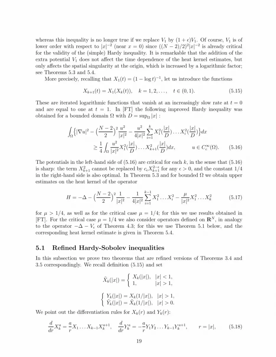
whereas this inequality is no longer true if we replace V1 by (1 + ǫ)V1. Of course, V1 is oflower order with respect to |x|−2 (near x = 0) since ((N − 2)/2)2|x|−2 is already criticalfor the validity of the (simple) Hardy inequality. It is remarkable that the addition of theextra potential V1 does not affect the time dependence of the heat kernel estimates, butonly affects the spatial singularity at the origin, which is increased by a logarithmic factor;see Theorems 5.3 and 5.4.

More precisely, recalling that X1(t) = (1 − log t)−1, let us introduce the functions

Xk+1(t) = X1(Xk(t)), k = 1, 2, . . . , t ∈ (0, 1). (5.15)

These are iterated logarithmic functions that vanish at an increasingly slow rate at t = 0and are equal to one at t = 1. In [FT] the following improved Hardy inequality wasobtained for a bounded domain Ω with D = supΩ |x| :

∫

Ω

|∇u|2 −(N − 2

2

)2 u2

|x|2−

u2

4|x|2

k∑

i=1

X21 (|x|

D) . . .X2

i (|x|

D)

dx

≥1

4

∫

Ω

u2

|x|2X2

1 (|x|

D) . . .X2

k+1(|x|

D)dx, u ∈ C∞

c (Ω). (5.16)

The potentials in the left-hand side of (5.16) are critical for each k, in the sense that (5.16)is sharp: the term X2

k+1 cannot be replaced by cǫX2−ǫk+1 for any ǫ > 0, and the constant 1/4

in the right-hand side is also optimal. In Theorem 5.3 and for bounded Ω we obtain upperestimates on the heat kernel of the operator

H = −∆ −(N − 2

2

)2 1

|x|2−

1

4|x|2

k−1∑

i=1

X21 . . .X

2i −

µ

|x|2X2

1 . . .X2k (5.17)

for µ > 1/4, as well as for the critical case µ = 1/4; for this we use results obtained in[FT]. For the critical case µ = 1/4 we also consider operators defined on RN , in analogyto the operator −∆ − Vǫ of Theorem 4.3; for this we use Theorem 5.1 below, and thecorresponding heat kernel estimate is given in Theorem 5.4.

5.1 Refined Hardy-Sobolev inequalities

In this subsection we prove two theorems that are refined versions of Theorems 3.4 and3.5 correspondingly. We recall definition (5.15) and set

Xk(|x|) =

Xk(|x|), |x| < 1,1, |x| > 1,

Yk(|x|) = Xk(1/|x|), |x| > 1,

Yk(|x|) = Xk(1/|x|), |x| > 0.

We point out the differentiation rules for Xk(r) and Yk(r):

d

drXak =

a

rX1 . . .Xk−1X

a+1k ,

d

drY ak = −

a

rY1Y2 . . . Yk−1Y

a+1k , r = |x|, (5.18)

19

valid for 0 < r < 1 and r > 1 respectively, which are easily proved by induction.As in Theorem 3.4, we assume that f is a non-negative, continuous and radially sym-

metric function on Bc satisfying (3.11), that is,

f(x) ≤ K|x|−2−σ, |x| ≥ 1,

for some σ,K > 0. For ǫ > 0 we also define

Vk,ǫ(x) =

(

N−22

)2|x|−2 + 1

4|x|−2 ∑k

i=1X21 (|x|) . . .X2

i (|x|), |x| < 1,

ǫf(x), |x| > 1.(5.19)

We then have

Theorem 5.1 Assume that k < N − 2 and define

ǫk,0 = infu∈H1(Bc)

∫

Bc |∇u|2dx− N−2+k2

∫

∂B u2dS

∫

Bc fu2dx. (5.20)

Then ǫk,0 > 0 and for ǫ ∈ (0, ǫk,0) there holds

∫

RN|∇u|2dx−

∫

RNVk,ǫu

2dx ≥ c(

∫

RN|u|2N/(N−2)(X1 . . . Xk+1)

2N−2N−2 dx

)(N−2)/N

, (5.21)

for all u ∈ C∞c (RN).

Remark. The constant ǫk,0 is optimal in the sense that inequality (5.21) fails for ǫ = ǫk,0.Also the exponent (2N − 2)/(N − 2) in (5.21) is sharp in the sense that it cannot bereplaced by a smaller exponent. The proof of these two facts is rather involved; see [FT]for similar arguments. We do not use these facts in the sequel.Proof. The proof follows closely that of Theorem 3.4, so we only give a sketch of it. Thepositivity of ǫk,0 follows from Lemma 2.4 (i), yielding ǫk,0 ≥ K−1µB((N − 2 + k)/2). Nowlet ǫ ∈ (0, ǫk,0) be fixed and let ψ be the radially symmetric solution to the problem

∆ψ + Vk,ǫψ = 0, |x| > 1,∂ψ∂ν

= −N−2+k2

ψ, |x| = 1,

normalized so that ψ = 1 on |x| = 1. The function

ψ(x) =

|x|−(N−2)/2X−1/21 . . .X

−1/2k , |x| < 1

ψ(x), |x| > 1,(5.22)

is then C1, radially symmetric and a direct computation which uses (5.18) shows that∆ψ+Vk,ǫψ = 0 in RN . Exactly as in Theorem 3.4, ψ is positive, radially symmetric and hasa positive limit as r → +∞. We then prove (5.21) in the case where u is radially symmetric,using once again Proposition 3.1. The validity of (5.21) for general u ∈ C∞

c (RN) followsfrom Lemma 3.3. //

20

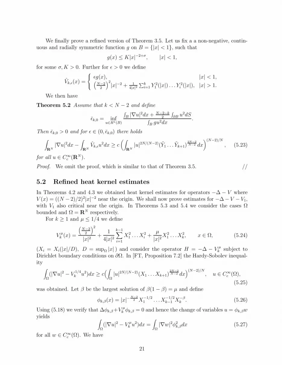
We finally prove a refined version of Theorem 3.5. Let us fix a a non-negative, contin-uous and radially symmetric function g on B = |x| < 1, such that

g(x) ≤ K|x|−2+σ, |x| < 1,

for some σ,K > 0. Further for ǫ > 0 we define

Vk,ǫ(x) =

ǫg(x), |x| < 1,(

N−22

)2|x|−2 + 1

4|x|2∑ki=1 Y

21 (|x|) . . . Y 2

i (|x|), |x| > 1.

We then have

Theorem 5.2 Assume that k < N − 2 and define

ǫk,0 = infu∈H1(B)

∫

B |∇u|2dx+ N−2−k2

∫

∂B u2dS

∫

B gu2dx

.

Then ǫk,0 > 0 and for ǫ ∈ (0, ǫk,0) there holds

∫

RN|∇u|2dx−

∫

RNVk,ǫu

2dx ≥ c(

∫

RN|u|2N/(N−2)(Y1 . . . Yk+1)

2N−2N−2 dx

)(N−2)/N

, (5.23)

for all u ∈ C∞c (RN).

Proof. We omit the proof, which is similar to that of Theorem 3.5. //

5.2 Refined heat kernel estimates

In Theorems 4.2 and 4.3 we obtained heat kernel estimates for operators −∆ − V whereV (x) = ((N − 2)/2)2|x|−2 near the origin. We shall now prove estimates for −∆− V − V1,with V1 also critical near the origin. In Theorems 5.3 and 5.4 we consider the cases Ωbounded and Ω = RN respectively.

For k ≥ 1 and µ ≤ 1/4 we define

V µk (x) =

(

N−22

)2

|x|2+

1

4|x|2

k−1∑

i=1

X21 . . .X

2i +

µ

|x|2X2

1 . . .X2k , x ∈ Ω, (5.24)

(Xi = Xi(|x|/D), D = supΩ |x| ) and consider the operator H = −∆ − V µk subject to

Dirichlet boundary conditions on ∂Ω. In [FT, Proposition 7.2] the Hardy-Sobolev inequal-ity

∫

Ω(|∇u|2 − V

1/4k u2)dx ≥ c

(

∫

Ω|u|2N/(N−2)(X1 . . .Xk+1)

2N−2N−2 dx

)(N−2)/N, u ∈ C∞

c (Ω),

(5.25)was obtained. Let β be the largest solution of β(1 − β) = µ and define

φk,β(x) = |x|−N−2

2 X−1/21 . . .X

−1/2k−1 X

−βk . (5.26)

Using (5.18) we verify that ∆φk,β+V µk φk,β = 0 and hence the change of variables u = φk,βw

yields∫

Ω(|∇u|2 − V µ

k u2)dx =

∫

Ω|∇w|2φ2

k,βdx (5.27)

for all w ∈ C∞c (Ω). We have

21

Theorem 5.3 Let Ω be bounded, 1 ≤ k < N − 2, and 0 < µ ≤ 1/4. The heat kernel ofH = −∆ − V µ

k satisfies the estimate

K(t, x, y) < ct−N/2φk,β(x)φk,β(y), t > 0, x, y ∈ Ω; (5.28)

here V µk is given by (5.24) and φk,β(x) by (5.26).

Proof. For the proof we distinguish two cases.(1) Case µ < 1/4. For w ∈ C∞

c (Ω) we have

∫

Ω|∇w|2φ2

k,βdx =∫

Ω|∇u|2dx−

∫

ΩV µk u

2dx

(by (5.16)) ≥ c(

∫

Ω(|∇u|2 − V

1/4k−1u

2)dx)

(by (5.25)) ≥ c(

∫

Ω|u|2N/(N−2)(X1 . . .Xk)

2N−2N−2 dx

)(N−2)/N

= c(

∫

Ω|w|2N/(N−2)|x|−N(X1 . . .Xk−1)X

2N−2−2Nβ

N−2

k dx)(N−2)/N

≥ c(

∫

Ω|w|2N/(N−2)φ2

k,βdx)(N−2)/N

.

This implies that Kφk,β(t, x, y) < ct−N/2 and (5.28) follows.

(2) Case µ = 1/4. By [FT, Lemma 7.5] the following Sobolev inequality holds

∫

Ω|∇w|2|x|2−NX−1

1 . . .X−1k dx ≥

≥ c(

∫

Ω|w|

2NN−2 |x|−NX1 . . . XkX

2N−2N−2

k+1 dx)(N−2)/N

, w ∈ C∞c (Ω).

This implies in particular

∫

Ω|∇w|2φ2

k,βdx ≥ c(

∫

Ω|w|

2NN−2φ2

k,βdx)(N−2)/N

, w ∈ C∞c (Ω)

and hence we have the uniform estimate Kφk,β(t, x, y) < ct−N/2 as required. //

We finally have the following consequence of Theorem 5.1, where we retain the notationof that theorem:

Theorem 5.4 Let 1 ≤ k < N − 2, and ǫ ∈ (0, ǫk,0) with ǫk,0 given by (5.20). the heatkernel of the operator −∆ − Vk,ǫ satisfies

K(t, x, y) < ct−N/2ψ(x)ψ(y), t > 0, x, y ∈ RN ;

here Vk,ǫ is given by (5.19) and ψ(x) by (5.22).

Proof. The result follows directly from Theorem 5.1 by means of (4.6). //

22

References

[AE] Adimurthi, Esteban M. J. An Improved Hardy-Sobolev Inequality in W 1,p and itsApplication to Schrodinger Operator. Preprint

[BV] Brezis H. and Vazquez J.-L. Blow-up solutions of some nonlinear elliptic problems.Rev. Mat. Univ. Comp. Madrid 10 (1997) 443-469.

[CKN] Caffarelli L.A., Kohn R. V. and Nirenberg L. First order interpolation inequalitieswith weights. Compositio Math. 53 (1984) 259-275.

[CM] Cabre X. and Martel Y. Existence versus instantaneous blowup for linear heatequations with singular potentials. C.R. Acad. Sci. Paris Ser. I Math. 329 (1999)973-978.

[D] Davies E.B. Heat kernels and spectral theory. Cambridge University Press 1989.

[DD] Davilla J. and Dupaigne L. Comparison Results for PDE’s with a Singular Poten-tial. Preprint 2001.

[DS] Davies E.B. and Simon B. Lp norms of non-critical Schrodinger semigroups. J.Funct. Anal. 102 (1991) 95-115.

[FT] Filippas S. and Tertikas A. Optimizing Improved Hardy inequalities. J. Funct. Anal.192 (2002) 186-233.

[G] Grigory’an A. Gaussian upper bounds for the heat kernel on arbitrary manifolds.J. Diff. Geom. 45 (1997) 33-52.

[LN] Li Y. and Ni W.-M. On conformal scalar curvature equations in RN . Duke Math.J. 57 (1988) 895-924.

[M] Maz’ya V. Sobolev spaces. Springer 1985.

[MS] Milman P. and Semenov Yu. Heat kernel bounds and desingularizing weights. J.Funct. Anal., to appear.

[T] Tertikas A. Critical phenomena in linear elliptic problems. J. Funct. Anal. 154(1998) 42-66.

[VZ] Vazquez J.L. and Zuazua E. The Hardy inequality and the asymptotic behaviourof the heat equation with an inverse-square potential. J. Funct. Anal. 173 (2000)103-153.

[WZ] Wang Zhi-Qiang and Zhu Meijun Hardy Inequalities with Boundary Terms.Preprint.

[Z] Zhang Q.S. Global bounds of Schrodinger heat kernels with negative potentials. J.Funct. Anal. 182 (2001) 344-370.

23