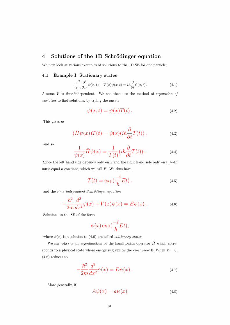
4 Solutions of the 1D Schrodinger equation

We now look at various examples of solutions to the 1D SE for one particle:

4.1 Example I: Stationary states

− �2

2m

∂2

∂x2ψ(x, t) + V (x)ψ(x, t) = i�

∂

∂tψ(x, t) . (4.1)

Assume V is time-independent. We can then use the method of separation of

variables to find solutions, by trying the ansatz

ψ(x, t) = ψ(x)T (t) . (4.2)

This gives us

(Hψ(x))T (t) = ψ(x)(i�∂

∂tT (t)) , (4.3)

and so1

ψ(x)Hψ(x) =

1

T (t)(i�

∂

∂tT (t)) . (4.4)

Since the left hand side depends only on x and the right hand side only on t, both

must equal a constant, which we call E. We thus have

T (t) = exp(−i

�Et) . (4.5)

and the time-independent Schrodinger equation

− �2

2m

d2

dx2ψ(x) + V (x)ψ(x) = Eψ(x) . (4.6)

Solutions to the SE of the form

ψ(x) exp(−i

�Et),

where ψ(x) is a solution to (4.6) are called stationary states.

We say ψ(x) is an eigenfunction of the hamiltonian operator H which corre-

sponds to a physical state whose energy is given by the eigenvalue E. When V = 0,

(4.6) reduces to

− �2

2m

d2

dx2ψ(x) = Eψ(x) . (4.7)

More generally, if

Aψ(x) = aψ(x) (4.8)

31

for some operator A and complex number a, then we say ψ(x) is an eigenfunc-tion of A with eigenvalue a. The terminology is a natural extension to infinite-dimensional spaces (of functions) of the definitions of eigenvector and eigenvaluefor finite-dimensional matrices: compare the eigenequation Av = av for matrix A,vector v and complex number a.

As we will see, the eigenvalues of physically significant operators are observablephysical quantities. They turn out always to be real – as we would expect, sincewe know of no natural way to directly observe a complex number in nature. Wewill see the mathematical reason for this when we discuss the general formalism ofquantum mechanics.

Notes

• Equation (4.7) has solution ei(kx−ωt), where E = �2k2

2m = �ω. This is thede Broglie wave we originally considered, so our discussion is at least self-consistent.

• This de Broglie wave solution to the 1D SE for a free particle is not normalis-able, and so does not have a well-defined probabilistic interpretation via theBorn rule. The quantum mechanical free particle is a very useful idealisa-tion, but not a physical solution. We never actually have a uniformly zeropotential throughout space, nor a single particle whose wavefunction is spreaduniformly over all of space. There could not be any consistent way of assign-ing probabilities to finding such a particle in finite regions, since there is nowell-defined uniform probability distribution on the 1D real line. (The sameis true in 3D, of course.)

• Any stationary state ψ(x, t) = ψ(x)e−iEt� has probability density

ρ(x, t) = |ψ(x, t)|2 = |ψ(x)|2 .

In other words, its probability density is time-independent. More generally,we will see the probability of measuring any given outcome for any dynamicalquantity is time-independent. Hence the name stationary state.

4.2 Completeness of the energy eigenfunctions

An important fact is that the general solution to the SE with t-independent potential

V (x) is a superposition of stationary states:

ψ(x, t) =∞�

n=1

anψn(x)e− iEnt

� . (4.9)

This follows from the fact that any wavefunction at a given time, say t = 0, can

be written as a superposition of energy eigenfunctions, so that,

ψ(x, 0) =∞�

n=1

anψn(x) , (4.10)

32

and from the linearity of the SE.We will see later (from theorem 6.3) that Eqn. (4.10) is a special case of the

more general result that any wavefunction can be written as a superposition ofeigenfunctions for any operator corresponding to a physically observable quantity.

If the set of energy eigenvalues is continuous, we need to replace the sum by

an integral. If there are continuous and discrete subsets, we need both sum and

integral. Thus if there is a discrete set of normalised energy eigenfunctions {ψi}Ni=1

(we includeN = ∞ as a possibility) and a continuous set of eigenfunctions {ψα}α∈Δ,

where the indexing set Δ is some sub-interval of the real numbers, we can write

ψ(x, t) =N�

n=1

anψn(x)e− iEnt

� +

�

Δ

aαψα(x)e− iEαt

� dα , (4.11)

33

4.3 Example II: Gaussian wavepackets

As an example of a continuous superposition of free particle stationary states,

consider

ψ(x, t) = C

� ∞

−∞e−

σ2 (k−k0)

2

ei(kx−�k22m t)dk . (4.12)

The exponent here is − 12 (σ + i�t

m )k2 + (k0σ + ix)k − σ2 k

20 , which we can write in

the form − 12a(k − b

a )2 + ( b

2

2a − σ2 k

20) , where a = σ + i�t

m , b = k0σ + ix.Now we have �

e−12a(k− b

a )2dk =

�2π

a. (4.13)

This gives us

ψ(x, t) = C ��

2π

σ + i�tm

exp((k0σ + ix)2

2(σ + i�tm )

) (4.14)

|ψ(x, t)|2 = C ���

1

σ2 + �2t2m2

exp((k0σ + ix)2

2(σ + i�tm )

+(k0σ − ix)2

2(σ − i�tm )

)

= C ���

1

σ2 + �2t2m2

exp(σ3k20 − σx2 + 2k0σx�t

m

σ2 + �2t2m2

)

= C ����

1

σ2 + �2t2m2

exp(−σ(x− k0�t

m )2

σ2 + �2t2m2

) , (4.15)

where C �, C �� and C ��� are constants.

Since

� ∞

−∞|ψ(x, t)|2dx = C ���

�2(σ2 + �2t2

m2 )π

2σ

�1

(σ2 + �2t2m2 )

= C ����

π

σ(4.16)

the normalisation condition gives us

C ��� =

�σ

π. (4.17)

Notes:

• The Gaussian wavepacket describes an approximately localised particle, almostall of whose probability density is within a finite region of size ≈ N(σ2 +

34

�2t2

m2 )12σ− 1

2 at time t, for some smallish positive numberN .12 This follows sincethe probability density function is a Gaussian curve with standard deviation

(σ2 + �2t2

m2 )12σ− 1

2 .

• Recall that we obtained the Gaussian wavepacket as a superposition of sta-tionary states. Considering its evolution, we thus see that a superposition ofstationary states is not necessarily stationary, since the Gaussian wavepacket’sprobability density function varies with time.

• From Eqn. (4.15), we see the speed of the Gaussian wavepacket’s centre is≈ �k0

m . Since its standard deviation is

(σ2 +�2t2

m2)

12σ− 1

2 ≈ �tmσ

12

(4.18)

for large t, the speed at which it spreads in width is ≈ �mσ

12. Note that,

mathematically speaking, neither is necessarily bounded by the speed of lightc. This illustrates that the Schrodinger equation is non-relativistic – i.e. in-compatible with special relativity. If it was possible to produce Gaussianwavepackets for any values of k0 and σ, and if the Schrodinger equation pre-cisely described their evolution, we could use the wavepackets to send signalsfaster than light.13

As this suggests, the SE is only approximately valid. 14 We cannot use Gaus-sian wavepackets (or, unless we find experimental evidence against specialrelativity, anything else) to send signals faster than light. However, the SEis a good enough approximation to allow us to understand a great deal ofphysics and chemistry.

• Pictures of an evolving Gaussian wave packet can be found at (for example)http://demonstrations.wolfram.com/EvolutionOfAGaussianWavePacket/

4.4 Example III: Particle in an infinite square potential well

Consider a particle confined by a 1D box with impermeable walls. We canmodel this by a potential

V (x) =

�0 |x| < a ,∞ |x| > a .

(4.19)

We look for stationary states obeying

− �2

2m

d2

dx2ψ(x) + V (x)ψ(x) = Eψ(x) , (4.20)

12For example, 99.7% of the probability density is within the region defined by N = 3.13We can also see that the SE is non-relativistic by noting that it is second order in x and first

order in t. A relativistically invariant equation must be of the same order in x and t, becauseLorentz transformations map x and t to linear combinations.

14Quantum mechanics, which is the topic of this course, is a non-relativistic theory, which isapproximately correct when relativistic corrections are small. Physicists tend to think of quantumtheory as defining a mathematical framework, and non-relativistic quantum mechanics as a par-ticular theory within this framework. The framework of quantum theory also includes relativisticquantum field theories, which (as the name suggests) are consistent with special relativity. Inparticular, there is a relativistically invariant equation for the evolution of an electron’s wavefunc-tion, from which the SE emerges as a non-relativistic limit. We won’t worry about relativisticcorrections or extensions of quantum mechanics in this course; they are discussed in Part III.

35

which gives us

− �2

2m

d2

dx2ψ(x) =

�Eψ(x) |x| < a ,(E −∞)ψ(x) |x| > a .

(4.21)

Here the second alternative is a useful but unrigorous shorthand, and should per-haps be written in quotation marks to emphasize this. The next paragraph explainshow we handle the infinity.

4.4.1 Handling discontinuities

We need a consistent treatment of discontinuities in V (x) and (hence perhaps)in ψ(x), dψ

dx , . . .. One method is to take a discontinuous V (x) as the limiting caseof a set of continuous potentials, and consider the limits of the solutions ψ(x). Butwe can address the SE with discontinuous V (x) directly using the following rules:

A step function discontinuity in ψ would create a delta function derivative ind2ψdx2 on the LHS of the SE, which would not be cancelled by other terms. So weexpect ψ to be continuous everywhere.

A step function discontinuity in dψdx would create a delta function in d2ψ

dx2 on theLHS of the SE; we can allow this only at points where V (x) is infinitely discontin-uous.

A step function discontinuity in d2ψdx2 gives a step function discontinuity on the

LHS of the SE; we can allow this only at points where V (x) has a finite step functiondiscontinuity so that the two discontinuities on the LHS cancel.

So, for the infinite square well we expect ψ to be continuous everywhere, anddψdx to be continuous except at |x| = a. Since V = ∞ for |x| > a, we need ψ = 0 inthis region for consistency of the SE. We have

ψ(x) = A cos(kx)+B sin(kx) , k =

�2mE

�2in |x| < a .

(4.22)

Now ψ = 0 at x = ±a gives

A cos(ka)± B sin(ka) = 0 (4.23)

and hence

A cos(ka) = 0 and B sin(ka) = 0 . (4.24)

36

Hence

either A = 0 , sin(ka) = 0 ,

ψ(x) = B sin(kx) , k =nπ

2afor n ≥ 2 even .

or B = 0 , cos(ka) = 0 ,

ψ(x) = A cos(kx) , k =nπ

2afor n ≥ 1 odd .

(4.25)

This gives us solutions for

E = En =�2π2n2

8ma2for n = 1, 2, 3, . . . (4.26)

Notes:

• We have quantised (i.e. discrete) energies for the stationary states of the infi-nite square well. Cf. the Bohr atom – it begins to look plausible that quantummechanics could explain the apparent quantisation of physical states. Perhapsthe allowed electron orbits in the Bohr atom correspond to the stationarystates in a 3D Coulomb potential?15

• The solutions fall into two classes:

ψ(x) =

�ψ(−x) even parity ,−ψ(−x) odd parity .

(4.27)

15We will see later that the relationship is a bit more complicated, but the intuition is along theright lines.

37

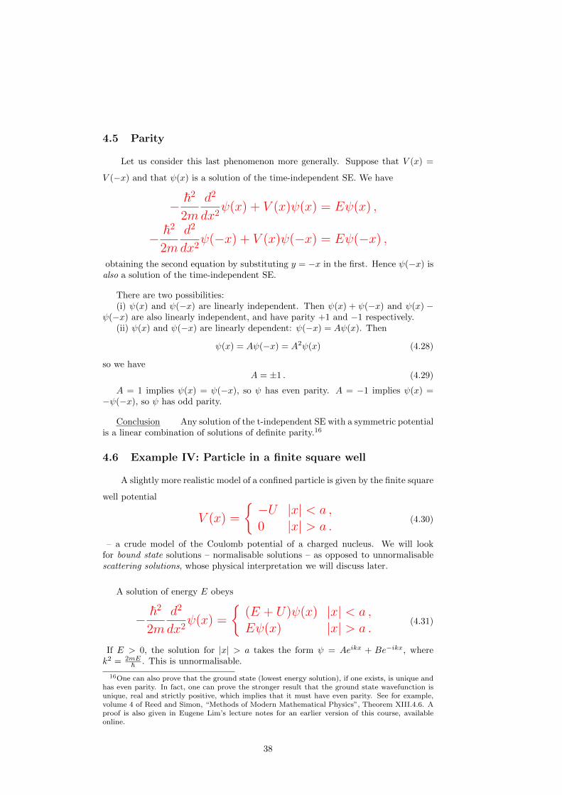
4.5 Parity

Let us consider this last phenomenon more generally. Suppose that V (x) =

V (−x) and that ψ(x) is a solution of the time-independent SE. We have

− �2

2m

d2

dx2ψ(x) + V (x)ψ(x) = Eψ(x) ,

− �2

2m

d2

dx2ψ(−x) + V (x)ψ(−x) = Eψ(−x) ,

obtaining the second equation by substituting y = −x in the first. Hence ψ(−x) isalso a solution of the time-independent SE.

There are two possibilities:(i) ψ(x) and ψ(−x) are linearly independent. Then ψ(x) + ψ(−x) and ψ(x) −

ψ(−x) are also linearly independent, and have parity +1 and −1 respectively.(ii) ψ(x) and ψ(−x) are linearly dependent: ψ(−x) = Aψ(x). Then

ψ(x) = Aψ(−x) = A2ψ(x) (4.28)

so we haveA = ±1 . (4.29)

A = 1 implies ψ(x) = ψ(−x), so ψ has even parity. A = −1 implies ψ(x) =−ψ(−x), so ψ has odd parity.

Conclusion Any solution of the t-independent SE with a symmetric potentialis a linear combination of solutions of definite parity.16

4.6 Example IV: Particle in a finite square well

A slightly more realistic model of a confined particle is given by the finite square

well potential

V (x) =

�−U |x| < a ,0 |x| > a .

(4.30)

– a crude model of the Coulomb potential of a charged nucleus. We will lookfor bound state solutions – normalisable solutions – as opposed to unnormalisablescattering solutions, whose physical interpretation we will discuss later.

A solution of energy E obeys

− �2

2m

d2

dx2ψ(x) =

�(E + U)ψ(x) |x| < a ,Eψ(x) |x| > a .

(4.31)

If E > 0, the solution for |x| > a takes the form ψ = Aeikx + Be−ikx, wherek2 = 2mE

� . This is unnormalisable.

16One can also prove that the ground state (lowest energy solution), if one exists, is unique andhas even parity. In fact, one can prove the stronger result that the ground state wavefunction isunique, real and strictly positive, which implies that it must have even parity. See for example,volume 4 of Reed and Simon, “Methods of Modern Mathematical Physics”, Theorem XIII.4.6. Aproof is also given in Eugene Lim’s lecture notes for an earlier version of this course, availableonline.

38

So we require E < 0. We will assume that E > −U , i.e. that |E| < U , since wedo not expect there to be solutions with energy lower than the minimum potential.

Exercise: Verify that indeed there are no such solutions.

Let

k2 =2m|E|�2

, (4.32)

l2 =2m(U − |E|)

�2, (4.33)

so that k2 + l2 =2mU

�2. (4.34)

For |x| > a we have

ψ(x) = Ae−kx + Bekx , (4.35)

and normalisability implies that

ψ(x) =

�Ae−kx x > a ,Bekx x < −a .

(4.36)

For |x| < a we have

ψ(x) = C cos(lx) +D sin(lx) . (4.37)

Since we know that the states of definite parity span the space of all boundstates, we can solve separately for even and odd parity states to get a completespanning set of solutions.

Consider the even parity solutions. If ψ(x) = ψ(−x) we have:

ψ(x) =

Ae−kx x > a ,Aekx x < −a ,C cos(lx) |x| < a.

(4.38)

ψ�(x) =

−kAe−kx x > a ,Akekx x < −a ,−lC sin(lx) |x| < a.

(4.39)

As ψ and ψ� are continuous at x = ±a, we find

C cos(la) = A exp(−ka) , (4.40)

−lC sin(la) = −kA exp(−ka) . (4.41)

39

This gives

k = l tan(la)

or(ka) = (la) tan(la) (4.42)

and from (4.34) we have

(ka)2 + (la)2 =2mUa2

�2. (4.43)

We can solve these last two equations graphically.The odd parity bound states (if any exist) can be similarly obtained.

The finite square well illustrates a general feature of quantum potentials V (x)such that V (x) → 0 as x → ±∞. The time-independent SE has two linearlyindependent solutions.

For E > 0, these take the form of scattering solutions

ψ(x) = A exp(ikx) + B exp(−ikx) as x → −∞C(A,B) exp(ikx) +D(A,B) exp(−ikx) as x → ∞ .

For E < 0, they have the form

ψ(x) = A exp(kx) + B exp(−kx) as x → −∞C(A,B) exp(kx) +D(A,B) exp(−kx) as x → ∞ .

Here C(A,B) and D(A,B) are linear in A and B, and depend also on k and onthe parameters defining V (x).

Only for special values of E < 0 can we find solutions such that B = 0 andC(A,B) = 0, as required for normalisability. For the remaining values of E < 0,the solutions blow up exponentially as x → −∞ or as x → ∞ (or both) and areunphysical: neither bound states nor scattering solutions.

[These asymptotically exponential functions are not physically meaningful: theyare not normalisable and do not define eigenfunctions of H.]

40

4.7 Example V: The quantum harmonic oscillator

has potential

V (x) =1

2mω2x2 . (4.44)

This is a particularly important example for several reasons.First, it is not only solvable but (as we will see later) has a very elegant solution

that explains some important features of quantum theory.Second, generic symmetric potentials in 1D are at least approximately described

by Eqn. (4.44). To see this, consider a potential V (x) taking a minimum value Vmin

at xmin and symmetric about xmin. Writing y = x− xmin, we have

V (y) = V (0) + yV �(0) +y2

2!V ��(0) +

y3

3!V ���(0) + . . .

≈ Vmin +y2

2!V ��(0) +O(y4) .

Renormalising the potential so that Vmin = 0, and taking V ��(0) = mω2, we recover(4.44). (If V ��(0) = 0 this argument does not hold, but even in this case the harmonicoscillator potential can be a good qualitative fit. See for example comments belowon approximating a finite square well potential by a harmonic oscillator potential.)

In fact, we can show something more general. Suppose we have a system with ndegrees of freedom that has a unique stable equilibrium. Then the small oscillationsabout equilibrium can be approximated by n independent harmonic oscillators. Thismeans that solving the harmonic oscillator allows us to give a quantum descriptionof molecules excited by radiation (and hence understand the greenhouse effect andmany other phenomena) and of the behaviour of crystals and other solids.

Third, the harmonic oscillator plays an even more fundamental role in quantumfield theory, where we understand particles as essentially harmonic oscillator exci-tations of fields. Our entire understanding of matter and radiation is thus based onthe quantum harmonic oscillator!

To obtain the stationary states of the quantum harmonic oscillator we need to

solve

− �2

2m

d2

dx2ψ(x) +

1

2mω2x2ψ(x) = Eψ(x) . (4.45)

We define

y =

�mω

�x and α =

2E

�ω. (4.46)

We have

d2ψ

dy2− y2ψ = −αψ . (4.47)

If ψ ∼ exp(− 12y

2), then ψ� ∼ −y exp(− 12y

2) and ψ�� ∼ y2 exp(− 12y

2) to leadingorder, which means that ψ�� − y2ψ ∼ (y2 − y2) exp(− 1

2y2) satisfies (4.47) to leading

order. Similarly ψ ∼ yn exp(− 12y

2) satisfies (4.47) to leading order. This suggestsconsidering power series solutions of the form

41

ψ(y) = H(y)e−y2

2 , (4.48)

H(y) =∞�

m=0

amym , (4.49)

and trying to match the coefficients am to produce an exact solution.

From (4.47) we getψ�� + (α− y2)ψ = 0 (4.50)

and substituting from (4.48, 4.50) we get

d2

dy2(H exp(−y2

2)) + (α− y2)H exp(−y2

2) = 0 (4.51)

(H �� − 2yH � +Hy2 −H + (α− y2)H) exp(−y2

2) = 0 (4.52)

(H �� − 2yH � + (α− 1)H) exp(−y2

2) = 0 (4.53)

We have

H �(y) =∞�

m=0

mamym−1 , (4.54)

H ��(y) =∞�

m=0

m(m− 1)amym−2

=∞�

m=0

am+2(m+ 2)(m+ 1)ym . (4.55)

So from (4.53) we get

∞�

m=0

(am+2(m+ 2)(m+ 1)− am(2m+ 1− α))ym = 0 . (4.56)

This must be true for all y, so each coefficient of ym must vanish:

am+2 =(2m+ 1− α)

(m+ 2)(m+ 1)am for m = 0, 1, 2, . . . . (4.57)

which determines the am for m ≥ 2 in terms of a0 and a1.

42

For large m, (4.57) gives am+2 ≈ 2mam , which asymptotically describes the

coefficients of ey2

:

ey2

=∞�

n=0

1

n!y2n =

∞�

n=0

bnyn

(4.58)

where for n odd we have bn = 0 and for n even we have

bn+2 =1

n2 + 1

bn =2

n+ 2bn ≈ 2

nbn . (4.59)

So, if the power series is infinite, we expect

H(y) ≈ Cey2

for some nonzero constant C: i.e. that H(y)

Cey2 → 1 as y → ∞. This implies that

ψ(y) ≈ H(y)e−y2

2 ≈ Ce12y

2

, (4.60)

which is not normalisable.We can justify this rigorously by noting that, for any � > 0, there exists some

integer m0 such that for all m ≥ m0 we have

am+2

am>

2(1− �)

m. (4.61)

Hence we have thatH(y) > Ce(1−�)y2 − P (y) , (4.62)

where C = am0�= 0 and P (y) is a polynomial of degree ≤ m0. This implies that

there exists a y0 such that for all y ≥ y0 we have

|H(y)| > C

2e(1−�)y2

, (4.63)

and hence

|ψ(y)| > C

2e(

12−�)y2

. (4.64)

So indeed ψ(y) diverges as y → ∞, and in particular ψ is not normalisable.

We thus need the power series to be truncated to a polynomial in order to findnormalisable physical solutions. Again, we can consider fixed (even and odd) paritysolutions separately:

• Even parity: a0 �= 0, a1 = 0, α = 2m+1 for some evenm.

• Odd parity: a0 = 0, a1 �= 0, α = 2m + 1 for some oddm.

So the physical solutions are given by

α =2E

�ω= 2m+ 1 (m = 0, 1, 2, . . .) (4.65)

43

i.e.

E = (m+1

2)�ω (m = 0, 1, 2, . . .) . (4.66)

The harmonic oscillator has energy levels equally spaced, separated by �ω, withminimum (or zero-point) energy 1

2�ω.

The polynomials Hn(y) corresponding to the physical solutions with energy(n+ 1

2 )�ω are the Hermite polynomials of degree n. We can obtain them explicitly17

from (4.65), using conventional normalisations:

H0 = 1 , H1 = 2y ,H2 = 4y2 − 2 , H3 = 8y3 − 12y , . . . . (4.67)

The corresponding wavefunctions are thus (up to normalisation)

ψ0 = e−12y

2

,ψ1 = 2ye−12y

2

, . . . (4.68)

17In fact one can derive a general expression (see e.g. Schiff, “Quantum Mechanics”, 3rd edition):

Hn(y) = (−1)ney2 dn

dyne−y2

.

44