arX

iv:q

uant

-ph/

0011

116v

6 2

0 Ja

n 20

01

Revised on August 22, 2018

The Relaxation Method for Solving theSchrodinger Equation in Configuration Spacewith the Coulomb and Linear Potentials

Alfred Tang, Daniel R. Shillinglaw and George Nill

Physics Department, University of Wisconsin - Milwaukee,

P. O. Box 413, Milwaukee, WI 53201.

Emails: atang@uwm.edu, drshilli@uwm.edu, geonill@uwm.edu

Abstract

The non-relativistic Schrodinger equation with the linear and Coulomb potentials is solvednumerically in configuration space using the relaxation method. The numerical methodpresented in this paper is a plain explicit Schrodinger solver which is conceptually simpleand is suitable for advanced undergraduate research.

1

1 Introduction

This work came out of an undergraduate research project at the University of Wisconsin-Milwaukee. The analytical solution of the hydrogen atom is a typical topic in advancedundergraduate or beginning graduate quantum mechanics which utilizes the series expan-sion technique. The analytic solution does not only illustrate the mathematical approachof solving differential equations, it also provides a benchmark for testing numerical meth-ods. Initially the numerical solution of the hydrogen atom was intended to offer theundergraduate students in our department (the second and third authors of this paper)an opportunity to learn the elements of scientific computation and basic research strate-gies. The students began by learning the theory of partial differential equations, linuxprogramming in C, and basic numerical methods. In order to give the students a tasteof original theoretical research, they were asked to check the eigenvalues generated bya Nystrom momentum space code from a new paper with the configuration space codewhich they helped to develop. This paper documents the r-space code for the numericalsolution of the non-relativistic Schrodinger equation (NRSE) with the Coulomb and linearpotentials. It is hoped that this work is helpful to those students and teachers who wantto integrate numerical methods with a traditional quantum mechanics curriculum.

2 Schrodinger Equation in configuration Space

The basis of the wavefunction of the Schodinger equation in configuration space is takento be

φlm(r) =Rl(r)

rYlm(Ω) (1)

The radial part of the equation for a hydrogen atom is [1]

d2Rl

dr2+

[

2µ

h

(

E +e2

r

)

−l(l + 1)

r2

]

Rl = 0. (2)

A computer cannot integrate r from zero to infinity. Therefore we must map [0,∞) →[0, 1] by

r =x

1− x(3)

It implies thatdx

dr= (1− x)2. (4)

From now on, a new symbol for the radial wavefunction will be used, i.e. y ≡ Rl.To transform the Schrodinger equation to the new space, we first transform the second

2

derivative,

d2y

dr2=

dx

dr

d

dx

(

dx

dr

dy

dx

)

= (1− x)2d

dx

(

(1− x)2dy

dx

)

= (1− x)2[

2(1− x)dy

dx+ (1− x)2

d2y

dx2

]

(5)

By substituting Eq. [5] into Eq. [2] and letting h→ 1 and

e2 =1

137, µ = 0.5107208× 106 eV, (6)

in natural units, the Schrodinger equation is transformed as

d2y

dx2+

2

1− x

dy

dx+

1

(1− x)4

[

2µ(

E +1− x

xe2)

−(

1− x

x

)2

l(l + 1)

]

y = 0. (7)

With the benefit of hindsight, we know that the non-zero portion of the solution of Eq. [7]will be tightly bound to a narrow margin near x ∼ 0. In order to improve the numericalaccuracy and the quality of the plots, we like to focus on the non-zero portion of thesolutions. A new configuration variable z and a redefinition of x

z ≡r

a0, z =

x

1− x, (8)

where

a0 ≡h2

µe2= 2.6831879× 10−4 eV −1, (9)

are used to zoom into the small x region. Eq. [7] is modified as

d2y

dx2+

2

1− x

dy

dx+

1

(1− x)4

[

2µ a20

(

E +1− x

x

e2

a0

)

−(

1− x

x

)2

l(l + 1)

]

y = 0. (10)

3 Relaxation Method

The shooting method typically shoots from one boundary point to another using Runga-Kutta integration. In the case of the Schrodinger equation, the boundary points at x = 0and x = 1 are both singular. A one-point shoot will not converge when the code marchestoward a singularity. A two-point shoot marches from both boundary points at x = 0and x = 1 to match a third boundary point somwhere in between. Even if it works,two-point shoot requires too much a priori knowledge of the wavefunction. Furthermore

3

any Runga-Kutta based alogrithms, such as the shooting methods, will fail under normalcircumstances because either (1) the integration tends to blow up to infinity when shootingfrom x = 0 or (2) the integration is identically zero when shooting from x = 1, giventhe boundary conditions y(1) = y′(1) = 0. An embedded exponentially-fitted Runga-Kutta method [2] is reported to work. But it is beyond the scope of an undergraduateresearch project. The relaxation method, on the other hand, will in principle handle twosingular boundary points. In this paper, we adapt the relaxation codes used in Numerical

Recipes [9]. In order to establish a continuity between this paper and the said reference,the same notations are used.

The basic idea of the relaxation method is to convert the differential equation intoa finite difference equation. Error functions are then considered. For instance, the er-ror function at the k-th mesh point of the j-th differential equation (one of N coupleddifferential equations)

dyj

dx

∣

∣

∣

∣

∣

xk

= g(xk, y1, . . . , yN) (11)

is simply

Ej,k = yj,k − yj,k−1 − (xk − xk−1)g(xk, xk−1, y1,k, y1,k−1, . . . , yN,k, yN,y−1). (12)

The difference of Ej,k is approximated by a first order Taylor series expansion, such that

N∑

n=1

Si,n∆yn,k−1 +2N∑

n=N+1

Si,n∆yn−N,k = −Ei,k, (13)

where

Si,n =∂Ei,k

∂yn,k−1

, Si,n+N =∂Ei,k

∂yn,k. (14)

The crux of this paper is to show how the matrix elements Si,k of the non-relativisticSchrodinger equation are calculated and how to streamline the relaxation codes. Theranges of the sums in Eq [13] are split over [1, N ] and [N+1, 2N ] because of the peculiarityof the relaxation codes used in Numerical Recipes. We will not delve into the details ofthe codes in this paper. Readers are encouraged to refer to Numerical Recipes for a fullexplanation. As a motivation, it suffices to say that the main idea of the relaxation methodis to begin with initial guesses of yj,k and relax them to the approximately true valuesby calculating the errors Ei,k to correct yj,k iteratively. yj,k are components of a solutionvector in an NM-dimensional vector space. Intuitively we can think of the relaxationprocess as rotating an initial vector into another vector under the constraints of Ei,k.Since y = 0 is a trivial solution, the relaxation process has a tendency to diminish thosecomponents of the solution vector that correspond to the wavefunction and its derivative.We will return to this point later in the paper.

4

Let M − 1 be the number of mesh points and h is step size, then

h =1

M − 1, (15)

and

xk = (k − 1)h, (16)

yk ≡ y(xk). (17)

We define the vector yi as

y1 = y

y2 = y′

y3 = E

such that

y′1 = y2 (18)

y′2 = −2

1− xy2 −

1

(1− x)4

[

2µ a20

(

y3 +1− x

x

e2

a0

)

−(

1− x

x

)2

l(l + 1)

]

y1 (19)

y′3 = 0 (20)

A first order finite derivative at xk is given as

y′k =yk − yk−1

h. (21)

In the relaxation formalism, Ei,k are to be zeroed. In this case, it is easy to see thatEq. [18] can be rewritten as

E1,k = y1,k − y1,k−1 −h

2(y2,k + y2,k−1). (22)

The corresponding S1,j S-matrix elements are

S1,1 =dE1,k

dy1,k−1

= −1, (23)

S1,2 =dE1,k

dy2,k−1

= −h

2, (24)

S1,3 =dE1,k

dy3,k−1

= 0, (25)

S1,4 =dE1,k

dy1,k= 1, (26)

S1,5 =dE1,k

dy2,k= −

h

2, (27)

S1,6 =dE1,k

dy3,k= 0. (28)

5

Similarly, Eq. [19] is rewritten as

E2,k = y2,k − y2,k−1 +2h

1− xk+xk−1

2

(y2,k + y2,k−1

2) +

h(

1− xk+xk−1

2

)4

×[

2µ a20

(

y3,k + y3,k−1

2+

1− xk+xk−1

2xk+xk−1

2

e2

a0

)

−(

1− xk+xk−1

2xk+xk−1

2

)2

l(l + 1)

y1,k + y1,k−1

2. (29)

The associating S1,j S-matrix elements are

S2,1 =dE2,k

dy1,k−1

=h

2(

1− xk+xk−1

2

)4

[

2µ a20

(

y3,k + y3,k−1

2+

1− xk+xk−1

2xk+xk−1

2

e2

a0

)

−(

1− xk+xk−1

2xk+xk−1

2

)2

l(l + 1)

, (30)

S2,2 =dE2,k

dy2,k−1

= −1 +h

1− xk+xk−1

2

, (31)

S2,3 =dE2,k

dy3,k−1

=hµ a20

(

1− xk+xk−1

2

)4

y1,k + y1,k−1

2, (32)

S2,4 =dE2,k

dy1,k= S2,1, (33)

S2,5 =dE2,k

dy2,k

= 1 +h

1− xk+xk−1

2

, (34)

S2,6 =dE2,k

dy3,k= S2,3. (35)

At last, Eq. [20] is rewritten as

E3,k = y3,k − y3,k−1, (36)

6

and the associating S3,j matrix elements are

S3,1 =dE3,k

dy1,k−1

= 0, (37)

S3,2 =dE3,k

dy2,k−1

= 0, (38)

S3,3 =dE3,k

dy3,k−1

= −1, (39)

S3,4 =dE3,k

dy1,k= 0, (40)

S3,5 =dE3,k

dy2,k= 0, (41)

S3,6 =dE3,k

dy3,k= 1. (42)

At the first boundary point x = 0, we have n1 = 1. The boundary condition is y(0) = 0.It translates to

E3,1 = y1,1. (43)

The only non-zero S-matrix element is

S3,4 = 1. (44)

At the second boundary point x = 1, we have n2 = 2. The boundary conditions arey(1) = y′(1) = 0, or equivalently

E1,M = y1,M , (45)

E2,M = y2,M . (46)

The only non-zero matrix elements are

S1,4 = 1, (47)

S2,5 = 1. (48)

The hydrogen atom finite difference equation can be generalized to any Coulombpentential by substituting e2 → λC . To adapt the code to solve NRSE with a linearpotential, the only modifications needed are

1− x

xe2 → −

x

1− xλL, (49)

in Eq. [19],1− xk+xk−1

2xk+xk−1

2

e2 → −xk+xk−1

2

1− xk+xk−1

2

λL (50)

in Eqs. [29,30], and the omission of all a0 from the matrix elements.

7

4 Exact Solution of the Hydrogen Atom

The non-relativistic hydrogen atom is solved exactly by series expansion. The first fewradial wavefunctions are found to be [1]

R10(r) =1√πγ

3

2

1 r e−γ1r, (51)

R20(r) =1√πγ

3

2

2 r (1− γ1r) e−γ2r, (52)

R21(r) =1√πγ

5

2

2 r2 e−γ2r, (53)

where

γn ≡1

n a0(54)

With the redefinition of variable by Eqs. [8,9] and the omission of normalization constants,Eqs. [51–53] can be rewritten as

R10(z) ∼ z e−z, (55)

R20(z) ∼ z (1− z) e−z

2 , (56)

R21(z) ∼ z2 e−z

2 . (57)

Eqs. [55–57] will be used to test the relaxation codes in Section [6].

5 Exact S-state Solution for the Linear Potential

The S-state eigenvalue of the non-relativistic Schrodinger equation with a linear potentialcan be solved exactly in configuation space. We shall use the analytic results to check ournumerical results. The non-relativistic Schrodinger equation can be written as

(

d2

dr2+

2

r

d

dr

)

R− 2µ[λL r −E]R = 0. (58)

Let S ≡ r R, then Eq. [58] can be simplified as

d2

dr2S − 2µ[λL r −E]S = 0. (59)

Define a new variable

x ≡(

2µ

λ2L

)1

3

[λLr − E], (60)

8

such that Eq. [58] can be transformed as

S ′′ − xS = 0, (61)

which is the Airy equation. The solution which satisfies the boundary condition S → 0as x→ ∞ is the Airy function Ai(x). It is easy to show that the eigen-energy formula is

En = −xn

(

λ2L2µ

)1

3

, (62)

where xn is the n-th zero of the Airy function counting from x = 0 along −x. In refer-ence [10], the values λL = 5 and µ = 0.75 are used. In this case, the eigen-energy formulais

En = −2.554364772 xn. (63)

6 Numerical Results

The matrix elements in the routine difeq have been calculated in section 3. All but themain driver subroutines are left intact. The intial guesses of the wavefunction and itsderivative in the main driver program are just the square of the sine function and itsderivative. The codes of the modified driver programs,bohr.c and linear.c, and theassociating difeq.c are listed in the appendix of this paper. All the codes are written inC.

For large number of mesh points (1000 ≤ N ≤ 10000), the code generates smoothwavefunctions and energies which do not correspond to any eigen modes. An explicitSchrodinger solver is known to be conditionally unstable [3, 4]. This kind of instabilitiesmotivates numerical schemes such as the Numrov method [5], the symplectic scheme [6],microgenetic algoritm [7], and others [8]. For smaller number of mesh points (40 ≤ N ≤100), it is observed that the relaxed eigenvalues are largely similar to the initial guessesand that the smoothness of the relaxed eigenfunctions is very sensitive to the initialguesses of the eigenvalue values. Therefore we adopt the criterion that the smoothnessof the relaxed wavefunction picks out an initial guess as the correct eigenvalue when thenumber of mesh points is small enough. This criterion has certain a priori appeal becausewe expect a real physical wavefunction to be smooth. The reason for using the initialguess instead of the relaxed eigenvalue is based on the observation that the former ismore accurate than the latter when the code is calibrated using exact results. Table [1]illustrates the motivation of the smoothness criterion. The combination of a small numberof mesh points and the smoothness criterion is the simplest way to make the relaxationcode workable as an explicit Schrodinger solver.

Figs. [1–3] compare the relaxed and exact wavefunctions of the hydrogen atom forthe first few quantum numbers. The relaxed wavefunction typically has a vanishingly

9

small amplitude. It is explained by the tendency of the relaxation routine to relax thewavefunction to the trivial solution ψ = 0. In order to compare the relaxed and exactwavefunctions, the amplitude of the diminishing relaxed wavefunction is rescaled to matchthe exact wavefunction. Despite the large descrepancies between the relaxed and exactwavefunctions of the hydrogen atom in Figs. [1,2], both the relaxed and exact wavefunc-tions share the same basic features. Both relaxed wavefunctions satisfy the smoothnesscriterion. However, there are some difficulties in obtaining a smooth relaxed wavefunc-tion for Fig. [3]. The relaxed wavefunction in this case also has an unwelcomed kinkon the right hand side of the plot, which the exact wavefunction does not show. Hencethe relaxed and exact wavefunctions do not share the same features in this case. Thediscrepancy here is mostly due to degeneracy. The eigen-energy formula of the hydrgonatom [1]

Enl = −e2

2 a0

1

(n+ l)2(64)

reveals the degeneracy over the n and l quantum states. For example, E21 = E30 suchthat the wavefunctions of these two states are degenerate by virtue of having the sameeigenvalue. In principle, any linear combination of the degenerate solution vectors alsosatisfies the finite difference equation Eq. [10]. It also means that the relaxed wavefunctioncan be any linear combination of the degenerate wavefunctions. This problem will plaguethe numerical solutions of all degenerate states at higher n and l. Imperfect wavefucntionsis not a liability when the goal is to calculate the eigenvalues in the simplest possible way.In this case, the relaxed wavefunction is used merely as a guide to pick out the correcteigenvalue and not as a final product.

The situation of the numerical solution of the linear potential is slightly better.Figs [4,5] illustrate the relaxed wavefunctions of a linear potential compared to the exactwavefunctions. The wavefunctions of a linear potential are not degenerate. The relaxationmethod is expected to be relatively successful in the absence of degeneracy. In this paper,we use λL = 5GeV and µ = 0.75GeV. Table [2] lists the eigenvalues of the first few l

values in the case of the linear potential.

7 Conclusion

In this paper, we show how to circumvent the problem of conditional instability associatingwith an explicit Schrodinger solver when the relaxation method is used. The relaxationcode with the combination of small number of mesh points and the smoothness criteriongives good approximate eigenvalues in both the linear and Coulomb potential cases. Therole of the relaxed wavefunction is simply to guide the selection of the correct eigenvalueand is not used as an answer. More accurate eigenvalues can be obtained by solving themomentum space integral equation using the Nystrom method [11]. In this work, wehave solved only the non-relativistic Schrodinger equation with the linear and Coulomb

10

potentials. In the case of a relativistic equation, the Hamiltonian contains a kinetic term√p2 +m2 − m which is difficult to solve numerically with r-space codes. The p-space

solution using the Nystrom method on the other hand has the advantages of stability,accuracy and robustness over the r-space solution using the relaxation or shooting meth-ods. For these reasons, we prefer the p-space codes over the r-space codes for productionpurposes. Nevertheless, the r-space code is useful in checking the p-space results wheneverthe former is available. The numerical r-space calculation is a natural starting point forstudents to learn scientific computation because they would have already seen the exactr-space solutions in a traditional quantum mechanics curriculum. Since the numericalsolution of the hydrogen atom is not readily available in publications, it is hoped thatthe numerical method presented in this paper provides the simplest numerical scheme tosupplement the discussion of the Schrodinger equation in an advanced undergraduate orbeginning graduate quantum mechanics course.

8 Acknowledgment

We thank our advisor Prof. John W. Norbury for motivating this project.

References

[1] W. Greiner, Quantum Mechanics: An Introduction (Frankfurt: Springer, 1989), 201.

[2] G. Avdelas, T. E. Simos and J. Vigo-Aguiar, Computer Physics Communications,131, 52 (2000).

[3] T. Iitaka, Physical Review E, 49, 4684 (1994).

[4] S. Succi, Physical Review E, 53, 1969 (1996).

[5] G. Avdelas and T. E. Simos, Physical Review E, 62, 1375 (2000).

[6] X. S. Liu, X. Y. Liu, Z. Y. Zhou, P. Z. Ding and S. F. Pan, International Journal ofQuantum Chemistry, 79, 343 (2000).

[7] H. Nakanishi and M. Sugawara, Chemical Physics Letters, 327, 429 (2000).

[8] N. Watanabe and M. Tsukada, Physical Review E, 62, 2914 (2000).

[9] W. H. Press, S. A. Teukosky, W. T. Vetterling, B. P. Flannery, Numerical Recipes in

C (Cambridge: Cambridge, 1997).

[10] J. W. Norbury, D. E. Kahana and K. M. Maung, Canadian Journal of Physics, 70,86 (1992).

11

[11] A. Tang and J. W. Norbury, to be published.

12

9 Appendix

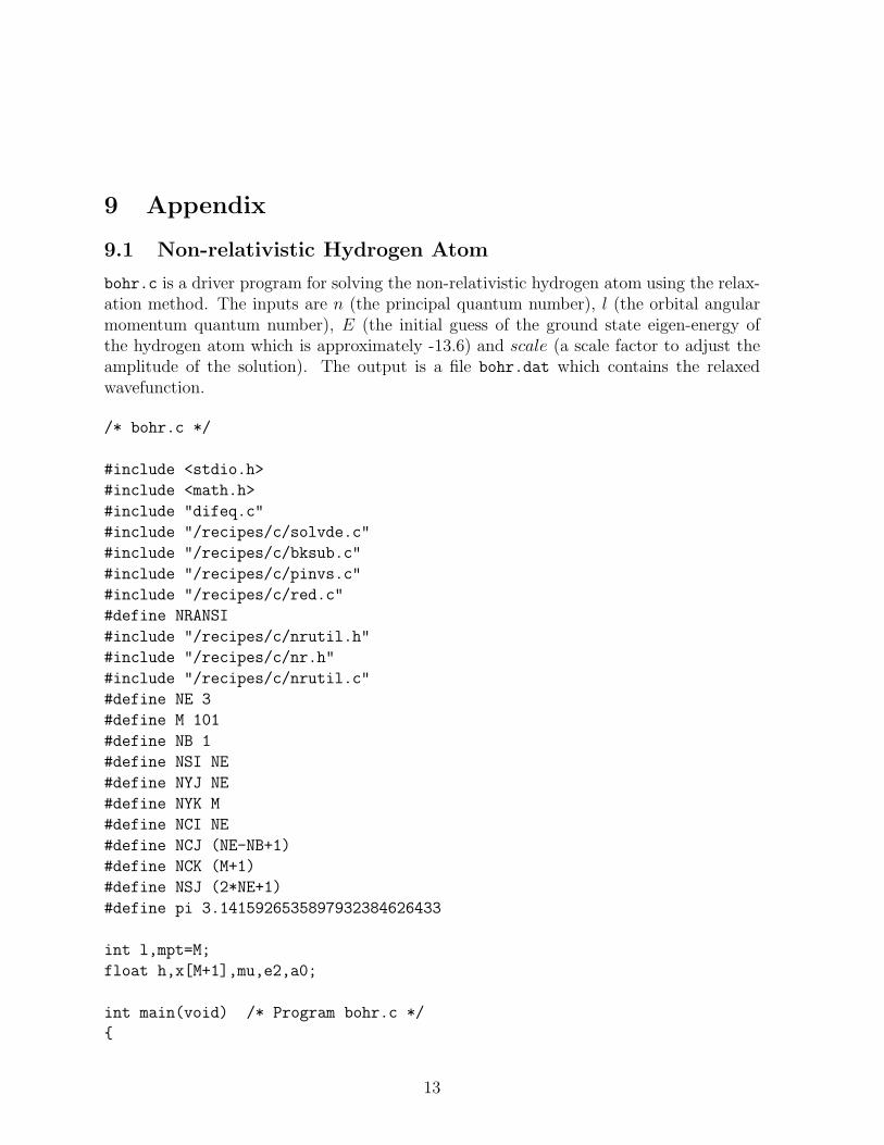
9.1 Non-relativistic Hydrogen Atom

bohr.c is a driver program for solving the non-relativistic hydrogen atom using the relax-ation method. The inputs are n (the principal quantum number), l (the orbital angularmomentum quantum number), E (the initial guess of the ground state eigen-energy ofthe hydrogen atom which is approximately -13.6) and scale (a scale factor to adjust theamplitude of the solution). The output is a file bohr.dat which contains the relaxedwavefunction.

/* bohr.c */

#include <stdio.h>

#include <math.h>

#include "difeq.c"

#include "/recipes/c/solvde.c"

#include "/recipes/c/bksub.c"

#include "/recipes/c/pinvs.c"

#include "/recipes/c/red.c"

#define NRANSI

#include "/recipes/c/nrutil.h"

#include "/recipes/c/nr.h"

#include "/recipes/c/nrutil.c"

#define NE 3

#define M 101

#define NB 1

#define NSI NE

#define NYJ NE

#define NYK M

#define NCI NE

#define NCJ (NE-NB+1)

#define NCK (M+1)

#define NSJ (2*NE+1)

#define pi 3.1415926535897932384626433

int l,mpt=M;

float h,x[M+1],mu,e2,a0;

int main(void) /* Program bohr.c */

13

void solvde(int itmax, float conv, float slowc, float scalv[],

int indexv[], int ne, int nb, int m, float **y, float ***c,

float **s);

int i,itmax,k,indexv[NE+1],n;

float conv,deriv,sinpx,cospx,q1,slowc,scalv[NE+1],eigen,guess;

float **y,**s,***c,max,scale;

FILE *fp;

mu=0.5107208e6;

e2=7.297353e-3;

a0=1.0/mu/e2;

y=matrix(1,NYJ,1,NYK);

s=matrix(1,NSI,1,NSJ);

c=f3tensor(1,NCI,1,NCJ,1,NCK);

itmax=100;

conv=1.0e-5;

slowc=1.0;

h=1.0/(M-1);

printf("\nn, l, E, scale = ");

scanf("%d%d%f%f",&n,&l,&guess,&scale);

indexv[1]=1;

indexv[2]=2;

indexv[3]=3;

for (k=1;k<=(M-1);k++)

x[k]=(k-1)*h;

sinpx=sin((n-l)*pi*x[k]);

cospx=cos((n-l)*pi*x[k]);

y[1][k]=sinpx*sinpx;

y[2][k]=2.0*(n-l)*pi*cospx*sinpx;

y[3][k]=guess/(l+n)/(l+n);

x[M]=1.0;

y[1][M]=0.0;

y[3][M]=guess/(l+n)/(l+n);

y[2][M]=0.0;

scalv[1]=1.0;

scalv[2]=1.0;

scalv[3]=-guess/(l+n)/(l+n);

solvde(itmax,conv,slowc,scalv,indexv,NE,NB,M,y,c,s);

eigen=-13.598289/(n+l)/(n+l);

printf("\nl\tE_in\t\tnumerical E\texact E\t\tnumerical-exact\n");

14

printf("%d\t%f\t%f\t%f\t%f\n\n",l,guess/(l+n)/(l+n),

y[3][1],eigen,y[3][1]-eigen);

fp=fopen("bohr.dat","w");

max=0.0;

for(i=1;i<=M;i++) if(fabs(y[1][i])>max) max=fabs(y[1][i]);

for(i=1;i<=M;i++) fprintf(fp,"%f\t%e\n",(i-1)*h,y[1][i]/max*scale);

fclose(fp);

free_f3tensor(c,1,NCI,1,NCJ,1,NCK);

free_matrix(s,1,NSI,1,NSJ);

free_matrix(y,1,NYJ,1,NYK);

return 0;

#undef NRANSI

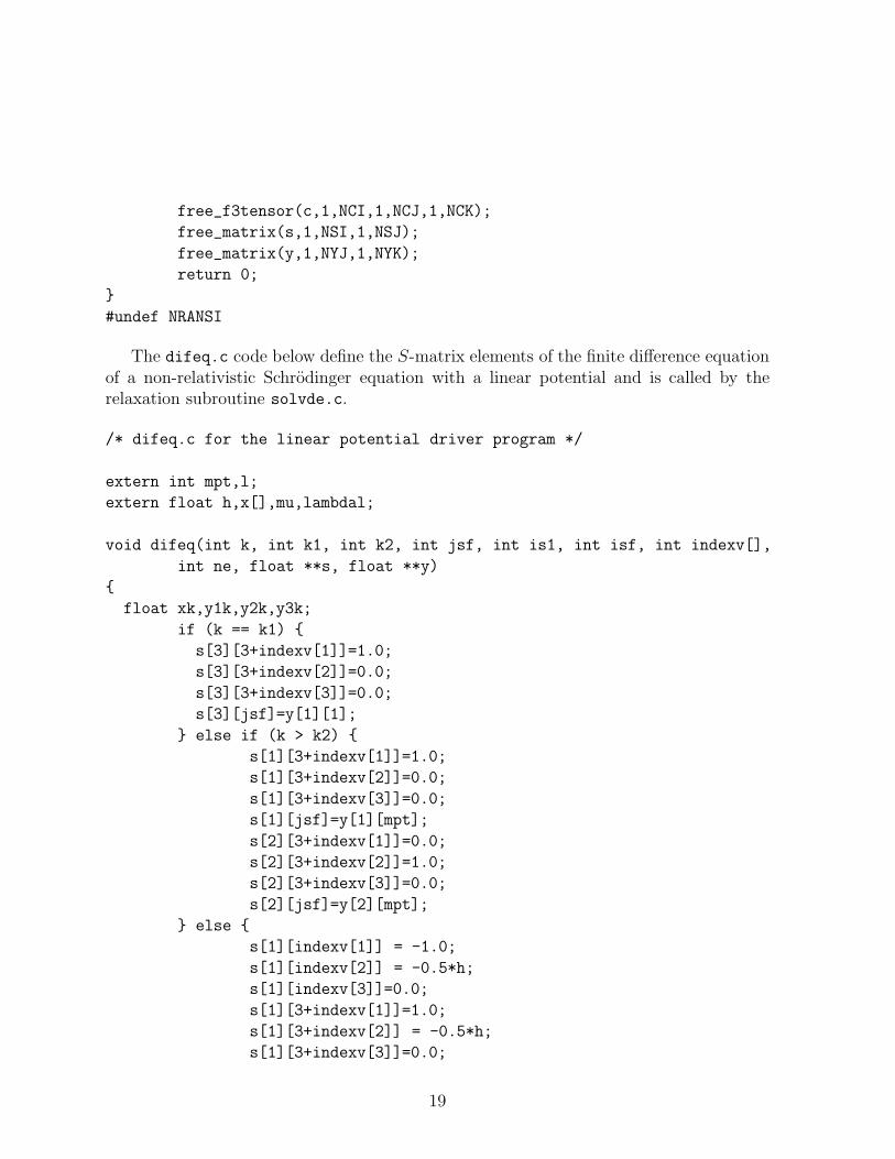
The difeq.c code below defines the S-matrix elements of the finite difference equationof the non-relativistic hydrogen atom and is called by the relaxation subroutine solvde.c.

/* difeq.c for the hydrogen atom driver program */

extern int mpt,l;

extern float h,x[],mu,e2,a0;

void difeq(int k, int k1, int k2, int jsf, int is1, int isf, int indexv[],

int ne, float **s, float **y)

float xk,y1k,y2k,y3k;

if (k == k1)

s[3][3+indexv[1]]=1.0;

s[3][3+indexv[2]]=0.0;

s[3][3+indexv[3]]=0.0;

s[3][jsf]=y[1][1];

else if (k > k2)

s[1][3+indexv[1]]=1.0;

s[1][3+indexv[2]]=0.0;

s[1][3+indexv[3]]=0.0;

s[1][jsf]=y[1][mpt];

s[2][3+indexv[1]]=0.0;

s[2][3+indexv[2]]=1.0;

s[2][3+indexv[3]]=0.0;

s[2][jsf]=y[2][mpt];

else

15

s[1][indexv[1]] = -1.0;

s[1][indexv[2]] = -0.5*h;

s[1][indexv[3]]=0.0;

s[1][3+indexv[1]]=1.0;

s[1][3+indexv[2]] = -0.5*h;

s[1][3+indexv[3]]=0.0;

xk=(x[k]+x[k-1])/2.0;

y1k=(y[1][k]+y[1][k-1])/2.0;

y2k=(y[2][k]+y[2][k-1])/2.0;

y3k=(y[3][k]+y[3][k-1])/2.0;

s[2][indexv[1]]=h/2.0/pow(1.0-xk,4.0)*

(2.0*mu*a0*a0*(y3k+(1.0/xk-1.0)*e2/a0)

-pow(1.0/xk-1.0,2.0)*l*(l+1));

s[2][indexv[2]] = -1.0+h/(1.0-xk);

s[2][indexv[3]]=h*mu/pow(1.0-xk,4.0)*y1k*a0*a0;

s[2][3+indexv[1]]=s[2][indexv[1]];

s[2][3+indexv[2]]=2.0+s[2][indexv[2]];

s[2][3+indexv[3]]=s[2][indexv[3]];

s[3][indexv[1]]=0.0;

s[3][indexv[2]]=0.0;

s[3][indexv[3]] = -1.0;

s[3][3+indexv[1]]=0.0;

s[3][3+indexv[2]]=0.0;

s[3][3+indexv[3]]=1.0;

s[1][jsf]=y[1][k]-y[1][k-1]-h*y2k;

s[2][jsf]=y[2][k]-y[2][k-1]+2.0*h/(1.0-xk)*y2k+

h/pow(1.0-xk,4.0)*(2.0*mu*a0*a0*(y3k+(1.0/xk-1.0)*e2/a0)

-pow(1.0/xk-1.0,2.0)*l*(l+1))*y1k;

s[3][jsf]=y[3][k]-y[3][k-1];

16

9.2 NRSE with a Linear Potential

linear.c is a driver program for solving the non-relativistic Schrodinger equation witha linear potential using the relaxation method. The inputs are n (the principal quantumnumber), l (the orbital angular momentum quantum number), E (the initial guess of theeigen-energy) and scale (a scale factor to adjust the amplitude of the wavefunction) Theoutput is a file linear.dat which contains the relaxed wavefunction.

/* linear.c */

#include <stdio.h>

#include <math.h>

#include "difeq.c"

#include "/recipes/c/solvde.c"

#include "/recipes/c/bksub.c"

#include "/recipes/c/pinvs.c"

#include "/recipes/c/red.c"

#define NRANSI

#include "/recipes/c/nrutil.h"

#include "/recipes/c/nr.h"

#include "/recipes/c/nrutil.c"

#define NE 3

#define M 101

#define NB 1

#define NSI NE

#define NYJ NE

#define NYK M

#define NCI NE

#define NCJ (NE-NB+1)

#define NCK (M+1)

#define NSJ (2*NE+1)

#define pi 3.1415926535897932384626433

int l,mpt=M;

float h,x[M+1],mu,lambdal;

int main(void)

void solvde(int itmax, float conv, float slowc, float scalv[],

int indexv[], int ne, int nb, int m, float **y, float ***c,

float **s);

int i,itmax,k,indexv[NE+1],n;

17

float conv,deriv,sinpx,cospx,q1,slowc,scalv[NE+1],max,e,scale;

float **y,**s,***c;

FILE *fp;

mu=0.75;

lambdal=5.0;

y=matrix(1,NYJ,1,NYK);

s=matrix(1,NSI,1,NSJ);

c=f3tensor(1,NCI,1,NCJ,1,NCK);

itmax=100;

conv=1.0e-6;

slowc=1.0;

h=1.0/(M-1);

printf("\nn, l, E scale = ");

scanf("%d%d%f%f",&n,&l,&e,&scale);

indexv[1]=1;

indexv[2]=2;

indexv[3]=3;

for (k=1;k<=(M-1);k++)

x[k]=(k-1)*h;

sinpx=sin(n*pi*x[k]);

cospx=cos(n*pi*x[k]);

y[1][k]=sinpx*sinpx;

y[2][k]=2.0*n*pi*cospx*sinpx;

y[3][k]=e;

x[M]=1.0;

y[1][M]=0.0;

y[3][M]=e;

y[2][M]=0.0;

scalv[1]=1.0;

scalv[2]=1.0;

scalv[3]=e;

solvde(itmax,conv,slowc,scalv,indexv,NE,NB,M,y,c,s);

fp=fopen("linear.dat","w");

max=0.0;

for(i=1;i<=M;i++) if (fabs(y[1][i])>max) max=fabs(y[1][i]);

for(i=1;i<=M;i++) fprintf(fp,"%f\t%f\n",(i-1)*h,y[1][i]/max*scale);

fclose(fp);

printf("\nl\tE_i\t\tE_f\n");

printf("%d\t%f\t%f\n\n",l,e,y[3][1]);

18

free_f3tensor(c,1,NCI,1,NCJ,1,NCK);

free_matrix(s,1,NSI,1,NSJ);

free_matrix(y,1,NYJ,1,NYK);

return 0;

#undef NRANSI

The difeq.c code below define the S-matrix elements of the finite difference equationof a non-relativistic Schrodinger equation with a linear potential and is called by therelaxation subroutine solvde.c.

/* difeq.c for the linear potential driver program */

extern int mpt,l;

extern float h,x[],mu,lambdal;

void difeq(int k, int k1, int k2, int jsf, int is1, int isf, int indexv[],

int ne, float **s, float **y)

float xk,y1k,y2k,y3k;

if (k == k1)

s[3][3+indexv[1]]=1.0;

s[3][3+indexv[2]]=0.0;

s[3][3+indexv[3]]=0.0;

s[3][jsf]=y[1][1];

else if (k > k2)

s[1][3+indexv[1]]=1.0;

s[1][3+indexv[2]]=0.0;

s[1][3+indexv[3]]=0.0;

s[1][jsf]=y[1][mpt];

s[2][3+indexv[1]]=0.0;

s[2][3+indexv[2]]=1.0;

s[2][3+indexv[3]]=0.0;

s[2][jsf]=y[2][mpt];

else

s[1][indexv[1]] = -1.0;

s[1][indexv[2]] = -0.5*h;

s[1][indexv[3]]=0.0;

s[1][3+indexv[1]]=1.0;

s[1][3+indexv[2]] = -0.5*h;

s[1][3+indexv[3]]=0.0;

19

xk=(x[k]+x[k-1])/2.0;

y1k=(y[1][k]+y[1][k-1])/2.0;

y2k=(y[2][k]+y[2][k-1])/2.0;

y3k=(y[3][k]+y[3][k-1])/2.0;

s[2][indexv[1]]=h/2.0/pow(1.0-xk,4.0)*(2.0*mu*

(y3k+xk/(xk-1.0)*lambdal)

-pow(1.0/xk-1.0,2.0)*l*(l+1));

s[2][indexv[2]] = -1.0+h/(1.0-xk);

s[2][indexv[3]]=h*mu/pow(1.0-xk,4.0)*y1k;

s[2][3+indexv[1]]=s[2][indexv[1]];

s[2][3+indexv[2]]=2.0+s[2][indexv[2]];

s[2][3+indexv[3]]=s[2][indexv[3]];

s[3][indexv[1]]=0.0;

s[3][indexv[2]]=0.0;

s[3][indexv[3]] = -1.0;

s[3][3+indexv[1]]=0.0;

s[3][3+indexv[2]]=0.0;

s[3][3+indexv[3]]=1.0;

s[1][jsf]=y[1][k]-y[1][k-1]-h*y2k;

s[2][jsf]=y[2][k]-y[2][k-1]+2.0*h/(1.0-xk)*y2k+

h/pow(1.0-xk,4.0)*(2.0*mu*(y3k+xk/(xk-1.0)*lambdal)

-pow(1.0/xk-1.0,2.0)*l*(l+1))*y1k;

s[3][jsf]=y[3][k]-y[3][k-1];

20

0 0.2 0.4 0.6 0.8 1

x

0

0.1

0.2

0.3

0.4

ψ(x

)

Exact

Numerical

Figure 1: The relaxed n = 1, l = 0 wavefunction of the non-relativistic hydrogen atomcompared against the exact wavefunction. The numerical eigenvalue is −13.59827 eV,versus the exact value of −13.598289 eV.

21

0 0.2 0.4 0.6 0.8 1

x

−1.5

−1

−0.5

0

0.5

1

1.5

2

ψ(x

)

Exact

Numerical

Figure 2: The relaxed n = 2, l = 0 wavefunction of the non-relativistic hydrogen atomcompared against the exact wavefunction. The numerical eigenvalue is −3.399750 eV,versus the exact value of −3.399572 eV.

22

0 0.2 0.4 0.6 0.8 1

x

0

0.5

1

1.5

2

2.5

3

ψ(x

)

Exact

Numerical

Figure 3: The relaxed n = 2, l = 1 wavefunction of the non-relativistic hydrogen atomcompared against the exact wavefunction. The numerical eigenvalue is −1.510056 eV,versus the exact value of −1.510921 eV.

23

0 0.2 0.4 0.6 0.8 1

x

0

0.1

0.2

0.3

0.4

0.5

ψ(x

)

Exact

Numerical

Figure 4: The relaxed l = 0, n = 1 state wavefunction of a non-relativistic Schrodingerequation with a linear potential using λL = 5GeV and µ = 0.75GeV. The numericaleigenvalue is 5.9719GeV, versus the exact value of 5.972379GeV. The relaxed wavefunc-tion has been rescaled to match the exact wavefunction.

24

0 0.2 0.4 0.6 0.8 1

x

−0.4

−0.2

0

0.2

0.4

0.6

ψ(x

)

Exact

Numerical

Figure 5: The relaxed l = 0, n = 2 state wavefunction of a non-relativistic Schrodingerequation with a linear potential using λL = 5GeV and µ = 0.75GeV. The numericaleigenvalue is 10.441GeV, versus the exact value of 10.442114GeV. The relaxed wave-function has been rescaled to match the exact wavefunction.

25

Table 1: Comparisons among the inital guesses, the relaxed and exact eigenvalues of thenon-relativistic hydrogen atom and the Schrodinger equation with a linear potential usingλL = 5GeV, µ = 0.75GeV.

Coulombn l Initial Numerical Exact1 0 -13.598270 -13.621142 -13.5982892 0 -3.399750 -3.400535 -3.3995722 1 -1.510056 -1.510060 -1.510921

Linearn l Initial Numerical Exact1 0 5.9719 6.146734 5.9723792 0 10.4410 10.418742 10.442114

26

Table 2: The numerical eigenvalues of the non-relativistic Schrodinger equation with alinear potential using λL = 5GeV, µ = 0.75GeV and n = 1.

l Numerical0 5.97191 8.58502 10.85143 12.90204 14.97905 16.5845

27