Rademacher sums from Weierstrass to QED

David Broadhurst, Open University, UK

Elliptics 19, Albert Einstein Institute, Potsdam18 September 2019

I give examples of situations in which Rademacher sums resolve thequestion of how to separate quasi-periods from periods.

At modular weight 2, I show how Rademacher sums restore to anelliptic curve a rational number lost by Weierstrass.

At higher genus, Rademacher sums emerge from hyper-elliptic curves.

Francis Brown encountered a Rademacher sum when studyingquasi-periods at weight 12 and level 1. I show how to extend this work upto weight 120, by taking Hadamard finite parts.

In QED, 4-loop radiative corrections to the magnetic moment of theelectron provide an example of quasi-periods, at weight 4 and level 6,resolved by a Rademacher sum.

A combination of two Rademacher sums appears in QED at 6 loops.

Plan:

1. Elliptic curves up to level 50:an integer that Weierstrass forgot.

2. Hyper-elliptic curves up to level 71:quasi-periods for the moonshine primes.

3. Quasi-periods at level 1:results up to weight 120.

4. Laporta’s 4-loop magnetic moment integrals:quasi-periods and Rademacher sums.

5. 6-loop QED.

1 Elliptic curves up to level 50

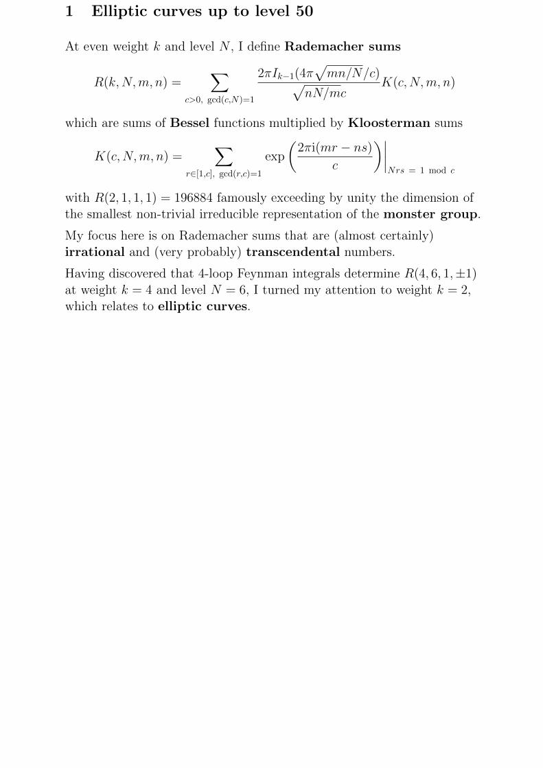
At even weight k and level N , I define Rademacher sums

R(k,N,m, n) =∑

c>0, gcd(c,N)=1

2πIk−1(4π√mn/N/c)√

nN/mcK(c,N,m, n)

which are sums of Bessel functions multiplied by Kloosterman sums

K(c,N,m, n) =∑

r∈[1,c], gcd(r,c)=1

exp

(2πi(mr − ns)

c

)∣∣∣∣Nrs = 1 mod c

with R(2, 1, 1, 1) = 196884 famously exceeding by unity the dimension ofthe smallest non-trivial irreducible representation of the monster group.

My focus here is on Rademacher sums that are (almost certainly)irrational and (very probably) transcendental numbers.

Having discovered that 4-loop Feynman integrals determine R(4, 6, 1,±1)at weight k = 4 and level N = 6, I turned my attention to weight k = 2,which relates to elliptic curves.

Karl Weierstrass (1815–1897) gave a beautifully concise definition of theperiods and quasi-periods of an elliptic curve y2 = 4x3 − g2x− g3.The periods, (ω+, ω−), come from integrals of dx/y.Weierstrass quasi-periods, (ηW+ , η

W− ), from integrals of xdx/y, satisfy

ω+ηW− − ω−ηW+ = 2πi, ηW+ ω+ =

π2

3G2

(−ω−ω+

),

G2(z) = 1− 24∑n>0

nqn

1− qn, q = exp(2πiz).

Now I restore an integer that Weierstrass forgot. Consider the quartic

y2 = Q(x) = x(x+ 4)(x+ 5)(x+ 9).

Its periods are delivered by the arithmetic-geometric mean of Gauss:

[agm(4, 5), agm(3, 5)] =

[2π

ω+,−2πi

ω−

]determining the weight 2 level 15 Rademacher sum

σ = R(2, 15, 1,−1) =agm(4, 5) agm(3, 5)

4π.

With a Rademacher sum ρ = R(2, 15, 1, 1), I define quasi-periods

η+ = (ρ+ σ)ω+, η− = (ρ− σ)ω−.

Pari/GP does not deliver these, since it is attuned to Weierstrass. Giventhe Cremona curve 15a1, it delivers quasi-periods ηW± = η±− 101

12 ω±, where101 is the integer that Weierstrass forgot. This is how it came about:

h4Q(1/h) = P (h) = (1 + 4h)(1 + 5h)(1 + 9h) = 180h3 + 101h2 + 18h+ 1

and then 101 is lost if we force the roots of the cubic to sum to zero.

In terms of Dedekind eta quotients, the cubic P (h) has a modularparametrization deriving from the level 15 cusp form f = η1η3η5η15:

h =1

5

(η53η5η51η15

− 1

)= q + 4q2 + 12q3 + 33q4 +O(q5)

d =q

f

dh

dq= 1 + 9q + 46q2 + 188q3 + 647q4 +O(q5)

d2 = P (h) = (1 + 4h)(1 + 5h)(1 + 9h), ηn = qn/24∏k>0

(1− qnk).

I have restored missing integers to all elliptic curves up to N = 50.

N class shift coeffs N class shift coeffs11 a 188 [1] 36 a 24 [1]14 a 109 [1] 37 a 60 [0, 1]15 a 101 [1] 37 b 100 [2, 1]17 a 81 [1] 38 a 457 [3, 0, 3]19 a 64 [1] 38 b −115 [1, 0,−1]20 a 52 [1] 39 a −127 [1, 0,−1]21 a 61 [1] 40 a 36 [2]24 a 44 [1] 42 a −79 [7/2,−1/2,−1]26 a −107 [1,−1] 43 a 82 [0, 1/2, 1/2]26 b 177 [1, 1] 44 a −20 [2,−1]27 a 36 [1] 45 a 57 [1, 1]30 a 13 [5/3,−1/3] 46 a −195 [7, 2,−5]32 a 24 [1] 48 a 28 [2]33 a 137 [2, 1] 49 a 21 [1]34 a 37 [5/2,−1/2] 50 a 13 [1]35 a 268 [1, 1, 1] 50 b 17 [1]

Table 1: Rademacher–Weierstrass shifts for elliptic curves with conductors up to N = 50.

Example: The Weierstrass quasi-periods of Cremona curve 33a1 areη± − 137

12 ω±, where η± are the quasi-periods determined by a combination2R(2, 33, 1, 1) +R(2, 33, 2, 1) of Rademacher sums, associated with

y2 = (x+ 11)(x+ 15)(4x+ 33) = 4x3 + 137x2 + 1518x+ 544.

2 Hyper-elliptic curves up to level 71

The majority of cusp forms of weight 2 are not of elliptic type. Considerfor example level N = 71, which is the largest prime that divides the orderof the monster group. Here we have a hyper-elliptic curve of genus 6and degree 14. A modular parametrization is achieved by

h =f6

f5 − 2f6= q − q3 − q4 + q6 +O(q8)

d =h5q

f6

dh

dq= 1 + 2q − 3q2 − 15q3 − 13q4 + 27q5 + 62q6 − 6q7 +O(q8)

d2 = P1(h)P2(h)

P1(h) = 1− 7h2 − 11h3 + 5h4 + 18h5 + 4h6 − 11h7

P2(h) = 1 + 4h+ 5h2 + h3 − 3h4 − 2h5 + h7

where fn = qn +O(q7) is a basis for the 6 cusp forms.

There are 6 pairs of periods and 6 pairs of quasi-periods to consider. The6 pairs of periods come from Eichler integrals of Hecke eigenformsFn =

∑6m=1 Tn,mfm where the entries of matrix T are constructed from

roots of the cubic x3 − x2 − 4x+ 3, with discriminant 257.

For each eigenform Fn, I constructed a weakly holomorphic modularform Gn such that periods of Fn and the quasi-periods of Gn determine apair of numbers (ρn, σn) in analogy with the elliptic case. These dependon an embedding of a number field. To transform them to Rademachersums, I use the transpose of the matrix T.

Example: At N = 35, with genus 3, I use

f = η25η27 = q +O(q6), h =

η1η35η5η7

= q +O(q2), d =q

f

dh

dq= 1 +O(q),

to parametrize a hyper-elliptic curve of degree 8

d2 = (1 + h− h2)(1− 5h− 9h3 − 5h5 − h6),

with a square root resolved by

d(z) = (1− 2h− h2)(η41η

45 − 72η47η

435

2f 2h

)−(η61η

67 − 53η65η

635

2f 3h

)= −d

(−1

35z

).

The space of cusp forms is spanned by [f1, f2, f3] = [1, h+ h2, h2]f , withfn = qn +O(q4). The space of weakly holomorphic forms is spanned by

g1 =1− 2h− 5h2 − 12h3 − 41h4 − d

2h2f = 35(2q4 + 2q5 + q6 +O(q7)),

g2 =1− hh

g1 − 70h2f = 35(6q4 + 7q5 + 9q6 +O(q7)),

g3 =1− 2h− h2

h2g1 − 70h(1 + 2h)f = 35(15q4 + 23q5 + 38q6 +O(q7)).

By construction gn(z) vanishes at the cusps at z = 135 ,

17 ,

15 , i∞.

It has an exponential singularity at small imaginary z, with

ε2gn

(iε√N

)=

1

Qn+O(Q), Q = exp

(−2π√Nε

).

It solves a recurrence relation for Rademacher sums:

∞∑m=1

R(2, N,m, n)qm = gn(z) +3∑

m=1

R(2, N,m, n)fm(z), for n = 1, 2, 3.

The Hecke eigenforms are given by the matrix equation F1

F2

F3

=

1 0 11 λ+ λ−1 λ− λ+

f1f2f2

, λ± =±√

17− 1

2.

Let T denote the matrix above. I seek matrices U and V such that

[G1, G2, G3] = [g1, g2, g3]UT−1 +N [f1, f2, f3]VT−1

are the weakly holomorphic eigenpartners of the eigenforms [F1, F2, F3].The eigenpartnership is as follows. Consider Eichler integrals

Pn =

∫ z2

z1

Fn(z)dz, Qn =

∫ z2

z1

Gn(z)dz, [z1, z2] =

[i− AN

,i +B

N

]along the horizontal path with =z = 1/N , with integers A and B suchthat AB ≡ 1 mod N . I require constants, ρn and σn, such that

=((Qn + ρnPn)Pn) = 0, =((Qn − σnPn)Pn) = 0,

R(2, N,+1, n) =3∑

m=1

ρmTm,n, R(2, N,−1, n) =3∑

m=1

σmTm,n.

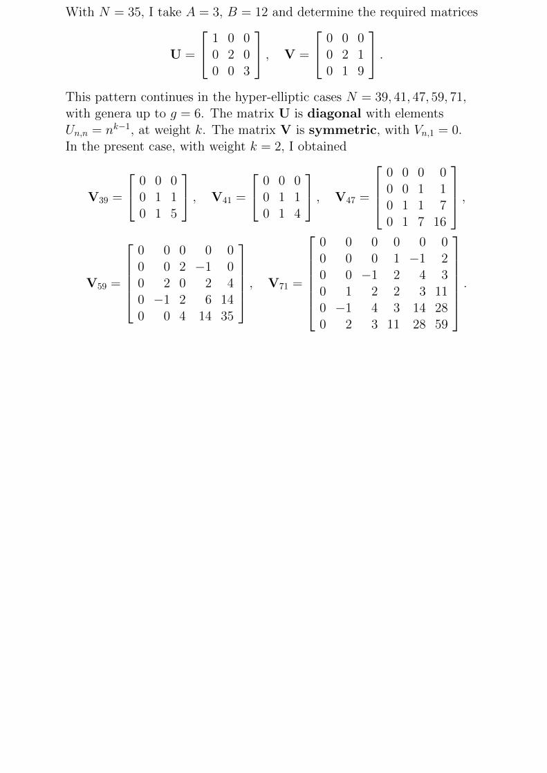
With N = 35, I take A = 3, B = 12 and determine the required matrices

U =

1 0 00 2 00 0 3

, V =

0 0 00 2 10 1 9

.This pattern continues in the hyper-elliptic cases N = 39, 41, 47, 59, 71,with genera up to g = 6. The matrix U is diagonal with elementsUn,n = nk−1, at weight k. The matrix V is symmetric, with Vn,1 = 0.In the present case, with weight k = 2, I obtained

V39 =

0 0 00 1 10 1 5

, V41 =

0 0 00 1 10 1 4

, V47 =

0 0 0 00 0 1 10 1 1 70 1 7 16

,

V59 =

0 0 0 0 00 0 2 −1 00 2 0 2 40 −1 2 6 140 0 4 14 35

, V71 =

0 0 0 0 0 00 0 0 1 −1 20 0 −1 2 4 30 1 2 2 3 110 −1 4 3 14 280 2 3 11 28 59

.

3 Quasi-periods at level 1 up to weight 120

Francis Brown posted ideas [arXiv:1710.07912] on quasi-periodsassociated to modular forms. A definition of these has been strangelyelusive at weights greater than 2. For the weight 12 level 1 cusp form

∆(z) = η241 = q∏n>0

(1− qn)24 =∆(−1/z)

z12

with q = exp(2πiz), periods are defined via L(∆, s) which has 11 criticalvalues at integers s ∈ [1, 11]. At odd integers these are given, up torational multiples of powers of π, by ω+, while at even integers we use ω−.Specifically, in terms of L(∆, 5) and L(∆, 6), the periods are

ω+ = −70(2π)11∫ ∞0

∆(iy)y4dy

= −68916772.8095951947543101246553310304390699691 . . .

ω− = −6(2π)11∫ ∞0

∆(iy)y5dy

= −5585015.37931040186687713926379627512963503343 . . .

Brown associates quasi-periods with the weakly holomorphic modularform ∆′(z), defined in terms of Klein’s j-invariant by

∆′(z) = (j2 − 1464j + 142236)∆(z) = 1/q +O(q2),

j =1

∆(z)

(1 + 240

∑n>0

n3qn

1− qn

)3

=1

q+ 744 + 196884q +O(q2)

Numerical values of

η+ = 127202100647.177094777317161298610877494045988 . . .

η− = 10276732343.6491327508171930724009209088993990 . . .

are obtainable from a determinant and permanent,

ω+η− − ω−η+ = (2π)1110!

ω+η− + ω−η+4πω+ω−

= −∑c>0

I11(4π/c)

c

∑r∈(Z/Zc)∗

exp

(2πi(r − s)

c

)∣∣∣∣∣∣rs=1mod c

with a Rademacher sum over Bessel functions and Kloosterman sums.

Integration of ∆′(z)zs−1dz along the imaginary axis z = iy requires one tohandle the singularity 1/q in ∆′ at large y, where q is small.

The indefinite integral of (log(q))s−1/q2 with respect to q is easilyperformed for integers s > 0. Then one simply drops singular terms at thelower limit q = 0 while retaining them at the involution point y = 1,corresponding to q = exp(−2π). For y < 1, the involution y → 1/y leadsto a similar prescription for the Hadamard finite part.

The quasi-period polynomial from integration of (X − zY )10∆′(z)dzhas a term X10 − Y 10, absent from the period polynomial.

From experience with Hecke eigenforms at level 71 and weight 2, I wasable to handle all level 1 cases up to weight 120, with 10 eigenforms.

The construction of 10 weakly holomorphic eigenpartners at weightk = 120 involves matrices with large integers. For example U10,10 = 10119,while V10,10 has 150 digits:

71743551479043323106025847609165970529550636954817\

15811526255378756621657659867939924492739540179038\

69536592195311460547291447667045944131309536870400.

4 The electron’s magnetic moment

The magnetic moment of the electron, in Bohr magnetons, has QEDcontributions

∑L≥0 aL(α/π)L given up to L = 4 loops by

a0 = 1 [Dirac, 1928]

a1 = 0.5 [Schwinger, 1947]

a2 = −0.32847896557919378458217281696489239241111929867962 . . .

a3 = 1.18124145658720000627475398221287785336878939093213 . . .

a4 = −1.91224576492644557415264716743983005406087339065872 . . .

Petermann and Sommerfield [1957] obtained

a2 =197

144+ζ(2)

2+

3ζ(3)− 2π2 log 2

4.

Laporta and Remiddi [1996] encountered U3,1 =∑

m>n>0(−1)m+n

m3n in

a3 =28259

5184+

17101ζ(2)

135+

139ζ(3)− 596π2 log 2

18

− 39ζ(4) + 400U3,1

24− 215ζ(5)− 166ζ(3)ζ(2)

24.

4.1 The first non-polylog

A Bessel moment

B = −∫ ∞0

27550138x+ 35725423x3

48600I0(x)K5

0(x)dx

= −1483.68505914882529459059985184510836700500152630607810 . . .

occurs at weight 4 in the breath-taking evaluation by Stefano Laporta[arXiv:1704.06996] of 4800 digits of

a4 = P +B+E +U ≈ 2650.565− 1483.685− 1036.765− 132.027 ≈ −1.912

where P comprises polylogs and E comprises integrals, with weights 5, 6and 7, whose integrands contain logs and products of elliptic integrals.U comes from 6 light-by-light master integrals, still under investigation.

The weight-4 non-polylog term B has N = 6 Bessel functions, with 5instances of K0(x), from 5-fermion intermediate states. The sibling ofK0(x) is I0(x) =

∑k≥0((x/2)k/k!)2, from Fourier transformation.

Both master integrals in B occur in D = 2 spacetime dimensions.

4.2 A simple determinant of Bessel moments

Consider Bessel moments of the form

M(a, b, c) =

∫ ∞0

Ia0 (x)Kb0(x)xcdx.

2LM(1, L+ 1, 1) is an L-loop sunrise integral at D = 2, on shell:

SL(t) =

∫ ∞0

dx1x1

. . .

∫ ∞0

dxLxL

1

(1 +∑L

j=1 xj)(1 +∑L

k=1 1/xk)− t

S4(1) = 24M(1, 5, 1) = 24∫ ∞0

I0(x)K50(x)xdx.

Laporta encountered M(1, 5, 1) as a master integral at D = 4. He alsoencountered M(1, 5, 3), which is obtained by differentiation of S4(t) beforesetting t = 1. Now look at the simple determinant

det

[M(1, 5, 1) M(1, 5, 3)M(2, 4, 1) M(2, 4, 3)

]=

π4

242

M(2, 4, 1) comes from cutting an internal line. It occurred at stages ofLaporta’s ε-expansions. M(2, 4, 3) comes from a cut and differentiation.

With q = exp(2πiz) and =(z) > 0, the Dedekind eta function satisfies

η(z) = q1/24∞∏n=1

(1− qn) =∞∑

n=−∞(−1)nq(6n+1)2/24 =

η(−1/z)√−iz

.

With ηn = η(nz) I define the weight-4 level-6 cusp form

f4,6(z) = (η1η2η3η6)2 =

∑n>0

A6(n)qn =f4,6(−1/(6z))

62z4.

For <s > 5/2, there is a convergent L-series

L6(s) =∑n>0

A6(n)

ns=

1

1 + 21−s1

1 + 31−s

∏p>3

1

1− A6(p)p−s + p3−2s.

Its analytic continuation is provided by the Eichler integral

L6(s) =(2π)s

Γ(s)

∫ ∞0

f4,6(iy)ys−1dy

with critical values related to Bessel moments as follows

L6(2) =2

π2M(1, 5, 1) =

2

3M(3, 3, 1), L6(1) =

2

π2M(2, 4, 1) =

3

π2L6(3).

4.3 Quasi-periods in QED

At weight 12 and level 1, the Eichler integrals for the quasi-periods of∆′(z) blow up exponentially as z → i∞ and as z → 0. I resolved thatissue by taking Hadamard finite parts. At weight 4 and level 6, inQED, the quasi-periods come from convergent Eichler integrals

D2

2=M(1, 5, 1)

π4=

4M(1, 5, 3)

π4+

5E2

183D1

5=M(2, 4, 1)

π3=

4M(2, 4, 3)

π3+E1

3[Ds

Es

]= −

∫ ∞1/√3

[f4,6(1+iy2

)g4,6(1+iy2

) ] ys−1dy,g4,6 =

(w2 − 3)2(w4 + 9)f4,68w4

= 5q + 102q2 + 945q3 +O(q4),

w = 3η22η

43

η41η26

, f4,6 = q − 2q2 − 3q3 +O(q4),

D1E2 −D2E1 =1

24π3,

satisfying the determinant criterion. What about the permanent?

4.4 Rademacher sums in QED

From ratios of Feynman integrals, I form

M(1, 5, 1) +M(1, 5, 3)

5M(1, 5, 1)=ρ− σ144

,M(2, 4, 1) +M(2, 4, 3)

5M(2, 4, 1)=ρ+ σ

144,

which I here relate to the Rademacher sums

ρ =∑

c=1,5mod 6

2πI3(4π/(√

6c))√6c

∑r∈(Z/Zc)∗

exp

(2πi(r −−− s)

c

)∣∣∣∣6rs=1mod c

σ =∑

c=1,5mod 6

2πJ3(4π/(√

6c))√6c

∑r∈(Z/Zc)∗

exp

(2πi(r +++ s)

c

)∣∣∣∣6rs=1mod c

=π4

40M(1, 5, 1)M(2, 4, 1)=

1

6(4π)3(f4,6, f4,6)= 0.8852376196 . . .

with an oscillating Bessel function J3(x) = iI3(ix) in σ, which isproportional to the inverse of the Petersson norm of the weight 4 level 6modular form f4,6. My evaluations of Feynman integrals determine 10,000decimal digits of ρ = 30.58572642 . . .. I conclude that the quasi-periodsare proportional to M(1, 5, 1) +M(1, 5, 3) and M(2, 4, 1) +M(2, 4, 3).

5 Quasi-periods in six-loop QED

Consider the Fourier expansion of the weight-6 level-6 cusp form

f6,6(z) =η92η

93

η31η36

+η91η

96

η32η33

=∑n>0

A8(n)qn = −f6,6(−1/(6z))

63z6.

For <s > 7/2, there is a convergent L-series

L8(s) =∑n>0

A8(n)

ns=

1

1− 22−s1

1 + 32−s

∏p>3

1

1− A8(p)p−s + p5−2s.

Its analytic continuation is provided by the Eichler integral

L8(s) =(2π)s

Γ(s)

∫ ∞0

f6,6(iy)ys−1dy

with critical values related to Bessel moments as follows

L8(4) =4

9π2M(1, 7, 1) =

4

9M(3, 5, 1) =

π2

9L8(2),

L8(5) =4

27M(2, 6, 1) =

2π2

21M(4, 4, 1) =

2π2

21L8(3) =

π4

54L8(1).

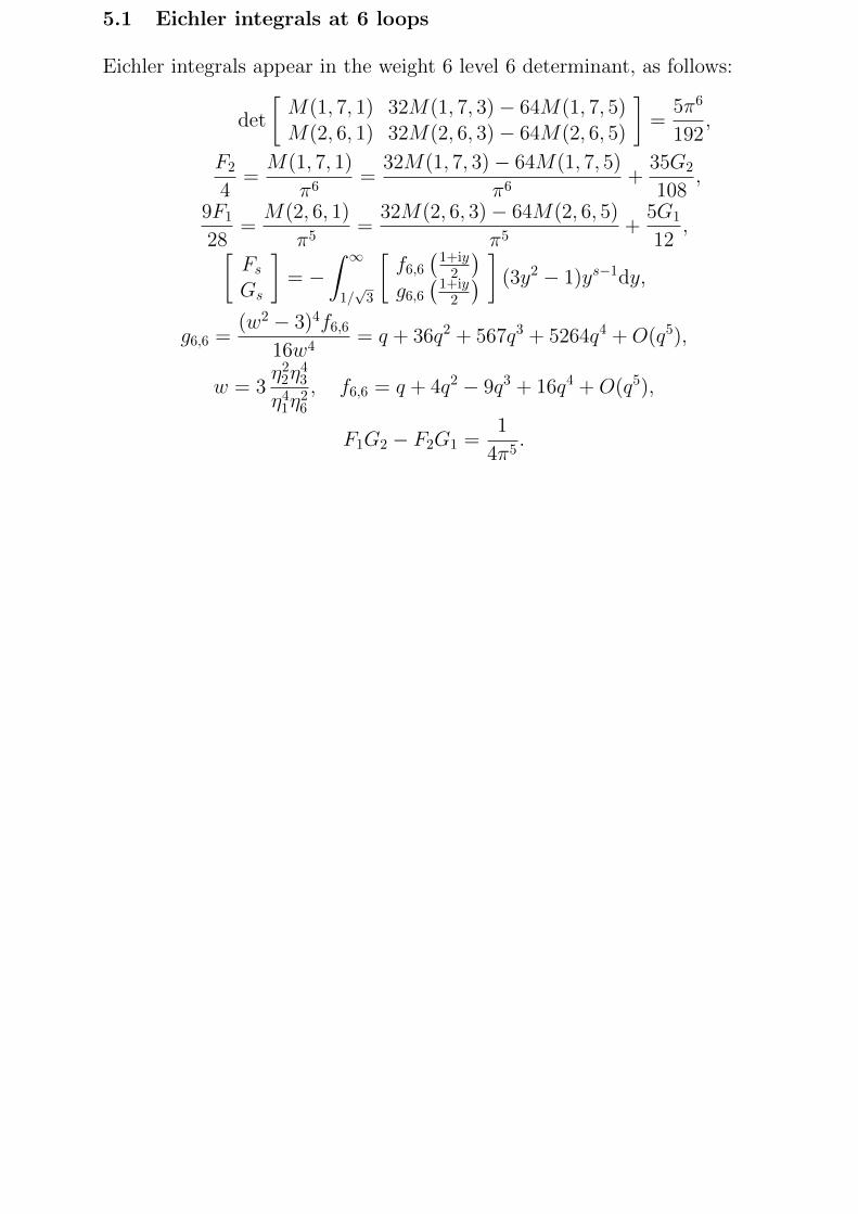
5.1 Eichler integrals at 6 loops

Eichler integrals appear in the weight 6 level 6 determinant, as follows:

det

[M(1, 7, 1) 32M(1, 7, 3)− 64M(1, 7, 5)M(2, 6, 1) 32M(2, 6, 3)− 64M(2, 6, 5)

]=

5π6

192,

F2

4=M(1, 7, 1)

π6=

32M(1, 7, 3)− 64M(1, 7, 5)

π6+

35G2

108,

9F1

28=M(2, 6, 1)

π5=

32M(2, 6, 3)− 64M(2, 6, 5)

π5+

5G1

12,[

Fs

Gs

]= −

∫ ∞1/√3

[f6,6(1+iy2

)g6,6(1+iy2

) ] (3y2 − 1)ys−1dy,

g6,6 =(w2 − 3)4f6,6

16w4= q + 36q2 + 567q3 + 5264q4 +O(q5),

w = 3η22η

43

η41η26

, f6,6 = q + 4q2 − 9q3 + 16q4 +O(q5),

F1G2 − F2G1 =1

4π5.

5.2 Rademacher sums at 6 loops

At weight 6 and level 6, there are two independent irrational Rademachersums in play. I found that

G1 + 9F1

F1+G2 + 9F2

F2=

2R(6, 6, 2, 1)− 5R(6, 6, 1, 1)

12.

It does not appear to be possible to determine any other combination ofR(6, 6, 2, 1) and R(6, 6, 1, 1) from 8-Bessel moments, since the relations

M(1, 7, 1) = 72M(1, 7, 3) + 7π4/48, M(2, 6, 1) = 72M(2, 6, 3)

lead to determinations of M(a, b, c) by periods and quasi-periods in thethe cases (a, b) = (1, 7) and (a, b) = (2, 6). Nor does the case (a, b) = (3, 5)yield essentially new numbers. Instead, the combination

3R(6, 6, 2, 1)− 3R(6, 6, 1, 1) = R(6, 3, 1, 1) + 35

indicates a connection to the old space at weight 6, coming from levelN = 3 and spanned by f6,3(z) = (η1η3)

6 and f6,3(2z) = (η2η6)6.

Conclusions

1. Rademacher sums define quasi-periods for elliptic curves, restoring aninteger that Weierstrass forgot.

2. In the hyper-elliptic cases at levels N = 35, 39, 41, 47, 59, 71, matrixtransformations relate Rademacher sums to Eichler integrals ofweakly holomorphic forms.

3. The most difficult case is level N = 1, since there are only two cuspsand the weakly holomorphic forms blow up, exponentially, at each.This problem was overcome by taking Hadamard finite parts, leadingto explicit relations between Rademacher sums and quasi-periods forall weights up to 120.

4. QED benefits neatly from level 6. At 4 loops, a Rademacher sumresolves the separation of quasi-periods from periods.

5. A combination of two Rademacher sums appears in QED at 6 loops.