Weierstrass traveling wave solutions for dissipative Benjamin, Bona, and Mahony(BBM) equationStefan C. Mancas, Greg Spradlin, and Harihar Khanal Citation: Journal of Mathematical Physics 54, 081502 (2013); doi: 10.1063/1.4817342 View online: http://dx.doi.org/10.1063/1.4817342 View Table of Contents: http://scitation.aip.org/content/aip/journal/jmp/54/8?ver=pdfcov Published by the AIP Publishing

This article is copyrighted as indicated in the abstract. Reuse of AIP content is subject to the terms at: http://scitation.aip.org/termsconditions. Downloaded to IP:

99.170.115.22 On: Sun, 24 Nov 2013 02:45:20

JOURNAL OF MATHEMATICAL PHYSICS 54, 081502 (2013)

Weierstrass traveling wave solutions for dissipativeBenjamin, Bona, and Mahony (BBM) equation

Stefan C. Mancas,a) Greg Spradlin,b) and Harihar Khanalc)

Department of Mathematics, Embry-Riddle Aeronautical University, Daytona-Beach,Florida 32114-3900, USA

(Received 21 February 2013; accepted 18 July 2013; published online 7 August 2013)

In this paper the effect of a small dissipation on waves is included to find exactsolutions to the modified Benjamin, Bona, and Mahony (BBM) equation by viscos-ity. Using Lyapunov functions and dynamical systems theory, we prove that whenviscosity is added to the BBM equation, in certain regions there still exist boundedtraveling wave solutions in the form of solitary waves, periodic, and elliptic func-tions. By using the canonical form of Abel equation, the polynomial Appell invariantmakes the equation integrable in terms of Weierstrass ℘ functions. We will use ageneral formalism based on Ince’s transformation to write the general solution ofdissipative BBM in terms of ℘ functions, from which all the other known solutionscan be obtained via simplifying assumptions. Using ODE (ordinary differential equa-tions) analysis we show that the traveling wave speed is a bifurcation parameter thatmakes transition between different classes of waves. C© 2013 AIP Publishing LLC.[http://dx.doi.org/10.1063/1.4817342]

I. INTRODUCTION

In 1895, Korteweg and de Vries, under the assumption of small wave amplitude and largewavelength of inviscid and incompressible fluids, derived an equation for the water waves, nowknown as the KdV equation,14 which also serves as a justifiable model for long waves in a wideclass of nonlinear dispersive systems. KdV equation has been also used to account adequately forobservable phenomena such as the interaction of solitary waves and dissipationless undular shocks.For the water wave problem Eq. (1.1) is nondimensionalized since the physical parameters u = 3η

2H ,

x =√

6x∗H , and t =

√6gH t∗, where η is the vertical displacement of the free surface, H is the depth

of the undisturbed water, x∗ is dimensional distance, and t∗ is the dimensional time are all scaledinto the definition of nondimensional space x, time t, and water velocity u(x, t). When the physicalparameters and scaling factors are appropriately absorbed into the definitions of u, x, and t, the KdVequation is obtained in the tidy form

ut + ux + uux + uxxx = 0. (1.1)

Although (1.1) shows remarkable properties it manifests non-physical properties; the mostnoticeable being unbounded dispersion relation. It is helpful to recognize that the main difficultiespresented by (1.1) arise from the dispersion term uxxx. The linearized version of (1.1), which doesnot include the nonlinear term, is

ut + ux + uxxx = 0. (1.2)

First, as noted in Ref. 5, when the solution of (1.2) is expressible as a summation of Fouriercomponents in the form F(k)ei(kx − ωt), the dispersion relation is ω(k) = k − k3, where ω(k) is the

a)mancass@erau.edu and stefan.mancas@erau.edub)spradlig@erau.educ)khana66a@erau.edu

0022-2488/2013/54(8)/081502/15/$30.00 C©2013 AIP Publishing LLC54, 081502-1

This article is copyrighted as indicated in the abstract. Reuse of AIP content is subject to the terms at: http://scitation.aip.org/termsconditions. Downloaded to IP:

99.170.115.22 On: Sun, 24 Nov 2013 02:45:20

081502-2 Mancas, Spradlin, and Khanal J. Math. Phys. 54, 081502 (2013)

frequency, and k is the wave number. The phase velocity C p = ω(k)k = 1 − k2 becomes negative for

k2 > 1, contrary to the original assumption of the forward traveling waves. More significantly, thegroup velocity Cg = dω

dk = 1 − 3k2 has no lower bound.To circumvent this feature, it has been shown by Peregrine,21 and later by Benjamin et al.5 that

(1.1) has an alternative format, which is called the regularized long-wave or Benjamin, Bona, andMahony (BBM) equation

ut + ux + uux − uxxt = 0, (1.3)

where the dispersion term uxxx is replaced by − uxxt to reflect a bounded dispersion relation. It iscontended that (1.3) is in important respects the preferable model over (1.1) which is not a suitablemodel for long waves.

The initial value problem for this equation has been investigated previously by Refs. 21–23,while the existence and stability of solitary waves have been investigated by Refs. 2,5,6,8, and 9. InRef. 5, Eq. (1.3) is recast as an integral equation, and its solutions global in time are found for initialdata in W 1,2(R). Also, the authors showed that its solutions have better smoothness properties thanthose of (1.1). In Ref. 8, global solutions are found for initial data in H s(R), s ≥ 0.

The linearized version of (1.3) has the dispersion relation ω(k) = k1+k2 , according to which

both phase and group velocities C p = 11+k2 and Cg = 1−k2

(1+k2)2 are bounded for all k. Moreover, bothvelocities tend to zero for large k, which implies that fine scale features of the solution tend not topropagate. The preference of (1.3) over (1.1) became clear in Ref. 5, when the authors attempted toformulate an existence theory for (1.1), respective to nonperiodic initial condition u(x, 0) defined on( − ∞, ∞).

A generalization to (1.3) to include a viscous term is provided by the equation

ut + ux + uux − uxxt = νuxx , (1.4)

where ν > 0 is transformed kinematic viscosity coefficient. The linearized version of (1.4) has

a complex dispersion relation w(k) = k−iνk2

1+k2 , so u(x, t) = eik(x− t1+k2 )e− νk2

1+k2 t . The real part of thefrequency coincides with the bounded dispersion relation of the nondissipative case, while theimaginary part contains the viscosity coefficient ν which must be positive to have decaying waves.In this case the harmonic solutions exhibit both dispersive and dissipative effects.

II. EXISTENCE OF DISSIPATIVE SOLUTIONS

In this section we propose an easy theorem based on dynamical system theory,4, 12 in whichwe prove the existence of solutions to (1.4) for both negative and positive traveling wave velocities(c < 0, c > 0). Also, we will show that the solution tends to the fixed points of the dynamical systemc − 1 ± k, for any k and large traveling wave variable ζ . We show that on boundaries the solutiondoes not necessarily decay to zero, but there is flow of energy through the boundaries to the solutionand back to the boundaries.

Theorem 1 below is proven by showing that a certain dynamical system in the plane has aheteroclinic orbit connecting two critical points. The Lyapunov function L is used to show that acertain trajectory of the dynamical system is bounded. The Poincare-Bendixson Theorem16 can beinferred to show that the trajectory approaches either a closed loop or a fixed point. The arguments inthe proof of Theorem 1 show that in the case of a closed loop, L would have to be constant along theloop, which is impossible by (2.12). Therefore, the trajectory must approach a fixed point instead,which we show is a function of the viscosity ν and velocity c.

An alternative to the dynamical systems approach to finding heteroclinic solutions to ODEssimilar to (2.3), perhaps with more complicated nonlinearities, are variational methods and critical

This article is copyrighted as indicated in the abstract. Reuse of AIP content is subject to the terms at: http://scitation.aip.org/termsconditions. Downloaded to IP:

99.170.115.22 On: Sun, 24 Nov 2013 02:45:20

081502-3 Mancas, Spradlin, and Khanal J. Math. Phys. 54, 081502 (2013)

point theory. There is an extensive literature on applying variational methods to these types ofequation without the dissipative term. See, for example, Ref. 7 and the references therein. Theinclusion of the dissipative term makes this approach more difficult. It is necessary to use morecomplicated function spaces and more complicated arguments, although this approach was usedsuccessfully in Ref. 3.

Theorem 1: Let c �= 0 and k > 0. (1.4) has a traveling wave solution of the form u(x, t) = u(x− ct) = u(ζ ) with u(ζ ) → (c − 1) + k as ζ → − ∞ and u(ζ ) → (c − 1) − k as ζ → ∞. If c <

0, then u(ζ ) < (c − 1) + k for all real ζ . If c > 0, then u(ζ ) > (c − 1) − k for all real ζ .

Proof: The class of soliton solutions is found by employing the form of the traveling wavesolutions of (1.4) which takes the form of the ansatz

u(x, t) = u(ζ ), (2.1)

where ζ ≡ x − ct is the traveling wave variable, and c is a nonzero translational wave velocity. Thesubstitution of (2.1) in (1.4) leads to

(1 − c)u′ + uu′ + cu′′′ = νu′′, (2.2)

where ′ = ddζ

. Integrating,

(1 − c)u + 1

2u2 + cu′′ = νu′ + A, (2.3)

for some constant A. With φ = u and ψ = u′, (2.3) is equivalent to the dynamical system

φ′ = ψ,

ψ ′ = ν

cψ + c − 1

cφ − 1

2cφ2 + A

c,

(2.4)

or

u′ = F(u) (2.5)

in vector notation. The fixed points of (2.4) are

z± =[

φ±

0

]=

[c − 1 ±

√(c − 1)2 + 2A0

]=

[c − 1 ± k

0

], (2.6)

for A = k2−(c−1)2

2 . We will show that (2.4) has a trajectory from z+ to z−.First, we will consider the c < 0 case. The linearization of (2.4) at z+ is

u′ =[

φ′

ψ ′

]=

⎡⎣ 0 1

−√

(c−1)2+2Ac

νc

⎤⎦

[φ − φ+

ψ

]≡ M

[φ − φ+

ψ

]. (2.7)

The determinant of M is negative, so z+ is a saddle point, and M has eigenvalues λ± with λ− < 0< λ+ .

The unit eigenvector corresponding to λ+ and pointing to the left is

v =

[−1

−λ+

]√

1 + (λ+)2. (2.8)

This article is copyrighted as indicated in the abstract. Reuse of AIP content is subject to the terms at: http://scitation.aip.org/termsconditions. Downloaded to IP:

99.170.115.22 On: Sun, 24 Nov 2013 02:45:20

081502-4 Mancas, Spradlin, and Khanal J. Math. Phys. 54, 081502 (2013)

Let g(ζ ) =[

g1(ζ )g2(ζ )

]be a solution of (2.4) with g(ζ ) → z+ and

∣∣∣ g(ζ ) − z+

|g(ζ ) − z+| − v∣∣∣ → 0 (2.9)

as ζ → − ∞. We will show that g(ζ ) → z− as ζ → ∞ and g1(ζ ) < φ + for all real ζ .Define

P3(φ) = 1

6φ3 + 1

2(1 − c)φ2 − Aφ. (2.10)

P3 is increasing on ( − ∞, φ − ], decreasing on [φ − , φ + ], and increasing on [φ + , ∞). Define

L(u) =P3(φ) − P3(φ+) + 1

2cψ2

=1

6φ3 + 1

2(1 − c)φ2 − Aφ − P3(φ+) + 1

2cψ2.

(2.11)

Then for all ζ ,

d

dζL(g(ζ )) =

(1

2g2

1 + (1 − c)g1 − A)

g′1 + cg2g′

2 =

=(1

2g2

1 + (1 − c)g1 − A)

g2+

cg2

(c − 1

cg1 − 1

2cg2

1 + ν

cg2 + A

c

)= νg2

2 ≥ 0.

(2.12)

Since L(z+) = 0 then L(g(ζ )) > 0 for all real ζ .Let φ − − < φ − with

P3(φ−−) < P3(φ+), (2.13)

and let

B = P3(φ−) − P3(φ+) = max{P3(φ) | φ−− ≤ φ ≤ φ+} − P3(φ+). (2.14)

Let L > 0 be large enough so that

1

2cL2 + B < 0, (2.15)

and define

R = (φ−−, φ+) × (−L , L). (2.16)

We claim that g(ζ ) ∈ R for all real ζ . As ζ → − ∞, g(ζ ) → z+ along the direction [1, λ+ ]T.Therefore, L(g(ζ )) > L(z+) = 0 for all real ζ , and there exists ζ ‘ ∈ R such that g(ζ ) ∈ R for all ζ

< ζ ‘.So, it suffices to show that L ≤ 0 on ∂R. Let u ∈ ∂ R. If φ = φ + , then L(u) = 1

2 cψ2 ≤ 0.Similarly, if φ = φ − − , then L(u) = P3(φ−−) − P3(φ+) + 1

2 cψ2 < 0. If φ − − ≤ φ ≤ φ + and ψ =L, then L(u) = P3(φ) − P3(φ+) + 1

2 cL2 ≤ B + 12 cL2 < 0. Similarly, if φ − − ≤ φ ≤ φ + and ψ =

− L, L(u) < 0.

This article is copyrighted as indicated in the abstract. Reuse of AIP content is subject to the terms at: http://scitation.aip.org/termsconditions. Downloaded to IP:

99.170.115.22 On: Sun, 24 Nov 2013 02:45:20

081502-5 Mancas, Spradlin, and Khanal J. Math. Phys. 54, 081502 (2013)

Define

L∞ = limζ→∞

L(g(ζ )). (2.17)

L∞ exists and is finite because L(g(ζ )) is a non-decreasing function of ζ , L is bounded on R, andg(ζ ) ∈ R for all real ζ . Let C be the ω-limit set of g, i.e.,

C = {u | ∃(ζm) ⊂ Rwith limm→∞ ζm = ∞, g(ζm) → u}, (2.18)

where C is nonempty because g(ζ ) ∈ R for all real ζ and R is bounded. C is compact and connected,and L = L∞ on C. We must prove C = {z−}.

Suppose C contains a point w that is not on the φ-axis. Then w is not a stationary point of (2.4),and C contains another point y. Let δ > 0 with δ < min(|w − y|, |w2|)/2. Then g crosses the annulusBδ(w) \ Bδ/2(w) infinitely many times, and there exist sequences (ζ m), (ζ ‘m) with ζ m → ∞ as m →∞, ζ m < ζ ‘m < ζ m + 1 for all m, |g(ζm) − w| = δ/2, |g(ζ ‘m) − w| = δ, and δ/2 < |g(ζ ) − w| < δ,for all m and all ζ ∈ (ζ m, ζ ‘m).

Let K = sup(|F(u)| | u ∈ Bδ(w)) < ∞, where F is from (2.5). Then ζ ‘m − ζ m ≥ δ/(2K) for allm. For ζ ∈ (ζ m, ζ ‘m),

d

dζL(g(ζ )) ≥ νg2

2(ζ ) ≥ νw22

4> 0, (2.19)

so

L(g(ζ ‘m)) − L(g(ζm)) =∫ ζ ‘m

ζm

d

dζL(g(ζ )) dζ ≥

∫ ζ ‘m

ζm

νw22

4dζ = ν(ζ ‘m − ζm)w2

2

4≥ δνw2

2

8K,

(2.20)

for all m. Therefore,

L∞ = L(g(ζ1)) + (L∞ − L(g(ζ1)) ≥

≥ L(g(ζ1)) +∞∑

m=1

L(g(ζ ‘m)) − L(g(ζm)) ≥

≥ L(g(ζ1)) +∞∑

m=1

δνw22

8K= ∞.

(2.21)

But L∞ is finite. This is a contradiction.Therefore, C is a subset of the φ-axis. Since C is connected and compact, C = [φ1, φ2] × {0}

for some φ − − < φ1 ≤ φ2 < φ + . Recall that L = L∞ on C. L is not constant on any segment ofthe φ-axis of positive length. So C is a single point, which is a stationary point of (2.4) in R. Thereis only one such point, z−.

Now consider the case c > 0. Let k > 0. Since − c < 0, we have seen that there exists g solving(2.2) with c replaced by − c, that is,

(1 + c)g′ + gg′ − cg′′′ − νg′′ = 0, (2.22)

with g(ζ ) → ( − c − 1) + k as ζ → − ∞, g(ζ ) → ( − c − 1) − k as ζ → ∞, and g(ζ ) < ( − c− 1) + k for all real ζ .

Define u : R → R by u(ζ ) = − g( − ζ ) − 2. Then g(ζ ) = − u( − ζ ) − 2, g′(ζ ) = u′( − ζ ),g′′(ζ ) = − u′′( − ζ ), and g′′′(ζ ) = u′′′( − ζ ). Substituting into (2.22) yields

0 = (1 + c)u′(−ζ ) + (−u(−ζ ) − 2)u′(−ζ ) − cu′′′(−ζ ) + νu′′(−ζ )

= (c − 1)u′(−ζ ) − u(−ζ )u′(−ζ ) − cu′′′(−ζ ) + νu′′(−ζ )

= −[(1 − c)u′(−ζ ) + u(−ζ )u′(−ζ ) + cu′′′(−ζ ) − νu′′(−ζ )].

(2.23)

This article is copyrighted as indicated in the abstract. Reuse of AIP content is subject to the terms at: http://scitation.aip.org/termsconditions. Downloaded to IP:

99.170.115.22 On: Sun, 24 Nov 2013 02:45:20

081502-6 Mancas, Spradlin, and Khanal J. Math. Phys. 54, 081502 (2013)

Therefore, u satisfies (2.2). By definition of u,

limζ→−∞

u(ζ ) = limζ→−∞

(−g(−ζ ) − 2) = limζ→∞

(−g(ζ ) − 2)

= −2 − limζ→∞

g(ζ ) = −2 − ((−c − 1) − k)

= (c − 1) + k

(2.24)

and

limζ→∞

u(ζ ) = limζ→∞

(−g(−ζ ) − 2) = limζ→−∞

(−g(ζ ) − 2)

= −2 − limζ→−∞

g(ζ ) = −2 − ((−c − 1) + k)

= (c − 1) − k.

(2.25)

For all real ζ , g(ζ ) < ( − c − 1) + k, so for all real ζ ,

u(ζ ) = −g(−ζ ) − 2 > −[(−c − 1) + k] − 2 = (c − 1) − k. (2.26)

Theorem 1 is proved.

III. EXACT SOLUTIONS VIA ℘ FUNCTIONS

A. Abel’s equation

The importance of Abel’s equation in its canonical forms stems from the fact that its integrabilityleads to closed form solutions to a general nonlinear ODE of the form

uζ ζ + q0(u)uζ + q2(u) = 0. (3.1)

This can be expressed by the following lemma.18

Lemma 1: Solutions to a general second order ODE of type (3.1) may be obtained via thesolutions to Abel’s equation (3.6), and vice versa using the following relationship

uζ = η(u(ζ )). (3.2)

Proof: To show the equivalence, one just needs the simple chain rule

uζ ζ = dη

duuζ = η

dη

du, (3.3)

which turns (3.1) into the second kind of Abel equation

dη

duη + q0(u)η + q2(u) = 0. (3.4)

Moreover, via transformation of the dependent variable

η(u) = 1

y(u), (3.5)

(3.4) becomes the Abel first kind without free or linear terms

dy

du= q0(u)y2 + q2(u)y3. (3.6)

This article is copyrighted as indicated in the abstract. Reuse of AIP content is subject to the terms at: http://scitation.aip.org/termsconditions. Downloaded to IP:

99.170.115.22 On: Sun, 24 Nov 2013 02:45:20

081502-7 Mancas, Spradlin, and Khanal J. Math. Phys. 54, 081502 (2013)

Comparing (3.1) with (2.3) we identify the constant, and quadratic polynomial coefficients

q0(u) = −ν

c,

q2(u) = u2

2c+ 1 − c

cu − A

c.

(3.7)

The need of dissipation is imperative since without the dissipation term q0 = 0, the Abel’s equation(3.6) becomes separable, as we will see next.

Progress of integration of (3.6) is based on the linear transformation v = ∫q0(u)du = − ν

c u,which allows us to write Abel’s equation (3.6) in canonical form

dy

dv= y2 + g(v)y3, (3.8)

where g(v) is the Appell’s invariant and is the quadratic polynomial

g(v) = − c2

2ν3v2 + c(1 − c)

ν2v + A

ν= a2v

2 + a1v + a0. (3.9)

By Lemke’s transformation17

y = −1

z

dz

dv, (3.10)

(3.8) can be written as a second-order differential equation with the preserved Appel’s invariantg(v),

z2 d2v

dz2+ g(v) = 0. (3.11)

B. No viscosity

If ν = 0 (2.3) becomes

uζ ζ = −u2

2c− 1 − c

cu + A

c. (3.12)

The classical solutions obtained before by Ref. 6 with the assumption that A = 0 are

u(x, t) = 3(c − 1)Sech2[√

c−1c

2(x − ct)

]if c > 1, (3.13)

u(x, t) = − 3c

1 + cSec2

[√c

2

(x − t

1 + c

)]if 0 < c < 1,

see left and middle panels of Fig. 1. Solitary waves that translate with velocity c > 1 are called fastwaves, while the periodic solutions that travel with velocity 0 < c < 1 slow waves.

FIG. 1. Traveling waves ν = 0, left c = 1.5 and middle c = 0.5, Eq. (3.13); right c = 1, Eq. (3.28).

This article is copyrighted as indicated in the abstract. Reuse of AIP content is subject to the terms at: http://scitation.aip.org/termsconditions. Downloaded to IP:

99.170.115.22 On: Sun, 24 Nov 2013 02:45:20

081502-8 Mancas, Spradlin, and Khanal J. Math. Phys. 54, 081502 (2013)

In (3.6) if let ν = 0, then the Abel’s equation

dy

du= q2(u)y3 (3.14)

is separable and leads to the elliptic algebraic equation

η2 = −u3

3c− 1 − c

cu2 + 2A

c− 2D. (3.15)

Using again the substitution uζ = η (3.15) becomes the elliptic differential equation

u2ζ = −u3

3c− 1 − c

cu2 + 2A

cu − 2D. (3.16)

For verification, if one takes ddζ

of the above, we recover (3.12).

Using a linear transformation, p. 311 of Ref. 11 of the dependent variable u = − 3√

12cu − (1 −c), (3.16) can be written in standard form

u2ζ = 4u3 − g2u − g3, (3.17)

with solution

u(ζ ) = ℘(ζ, g2, g3) (3.18)

and invariants

g2 = 3

√12

c2(c − 1)2 > 0, (3.19)

g3 =2(1 − c)3

3c. (3.20)

The limiting cases are obtained when A = 0, D = 0 to yield back to (3.13). We will not discuss herethis reduction to hyperbolic or trigonometric functions, since this was done extensible before bymany authors, but instead we refer the reader to Refs. 1 and 19 for the reduction and classificationthat depends on the sign of the invariants.

Instead, we will obtain a novel class of solutions that travel with a critical velocity c = 1. At theboundary between the fast and slow waves we will encounter periodic solutions in terms of rationalcombination of Jacobian elliptic functions.

If c = 1 and A = 0, Eq. (3.12) becomes

u2

2+ u′′ = 0. (3.21)

By multiplying by uζ and integrating once we obtain

u2ζ + u3

3= B3

3, (3.22)

where B is some nonzero constant of integration. In (3.15) if we let D = − B3

6 , we will also arrive to(3.22). Now let us use the substitution μ2 = B − u, where μ = μ(ζ ). Hence (3.22) is

μζ = ±√

3

6

√μ4 − 3Bμ2 + 3B2. (3.23)

Moreover, let us assume μ(ζ ) = 4√

3√

Bz(ζ ). Then (3.23) becomes

zζ = ±√

B

2 4√

3

√z4 −

√3z2 + 1. (3.24)

This ODE is solved using Jacobian elliptic functions.

This article is copyrighted as indicated in the abstract. Reuse of AIP content is subject to the terms at: http://scitation.aip.org/termsconditions. Downloaded to IP:

99.170.115.22 On: Sun, 24 Nov 2013 02:45:20

081502-9 Mancas, Spradlin, and Khanal J. Math. Phys. 54, 081502 (2013)

Claim 1: If Z = 1 + 2z2cos 2α + z4, then

u(x, k) =∫ x

0

dz√Z

= 1

2sn−1 2x

1 + x2,

with k = sin α, see p. 91 of Ref. 10.

Proof: Putting z = tan θ , we find

u(x, k) =∫ tan−1 x

0

dθ√1 − sin2 α sin2 2θ

,

followed by y = sin 2θ , which will give us

u(x, k) = 1

2

∫ 2x1+x2

0

dy√(1 − y2)(1 − k2 y2)

,

which is an elliptic integral of the first kind. Therefore, solving (3.24), we obtain the solution in z

2z

1 + z2= ±sn

(√B

4√

3ζ, k

), (3.25)

where k = sin 5π12 =

√3+1

2√

2is the modulus of the Jacobian elliptic function. It follows that for μ we

will have

2aμ

a2 + μ2= ±sn

(√3

3aζ, k

), (3.26)

where a = √B 4√

3. By solving the quadratic yields

μ = ±a1 ± cn

(√3

3 aζ, k)

sn(√

33 aζ, k

) . (3.27)

Therefore, the solution to the BBM equation without viscosity and velocity c = 1 is

u(x, t) =B[1 −

√3(1 ± cn

(√B

4√3(x − t), k

)sn

(√B

4√3(x − t), k

) )2]

=B[1 −

√3

1 ∓ cn(√

B4√3

(x − t), k)

1 ± cn(√

B4√3

(x − t), k)]

.

(3.28)

These critical solutions are 2K periodic with K obtained from the complete elliptic integral

K

2=

∫ 1

0

dz√z4 − √

3z2 + 1= 2.76806, (3.29)

see right panel of Fig. 1. The same solution was previously obtained by Cornejo-Perez and Rosu,using a factorization technique.24

The expressions (3.13) and (3.28) describe the whole class of solitary wave solutions withspectrum c ∈ (0, ∞) which is in concordance with Ref. 6. They present periodic and solitary wavesolutions to (1.3), with no restrictions on the constant A, which may be advantageous when adaptingresults to physical problems.

Remark 1: All the solutions obtained using simplifying assumptions ν = 0, A = 0 are particularcases of general solutions of (2.3) in terms of Weierstrass elliptic functions ℘, as we will see next.

This article is copyrighted as indicated in the abstract. Reuse of AIP content is subject to the terms at: http://scitation.aip.org/termsconditions. Downloaded to IP:

99.170.115.22 On: Sun, 24 Nov 2013 02:45:20

081502-10 Mancas, Spradlin, and Khanal J. Math. Phys. 54, 081502 (2013)

C. Viscosity present, ν > 0

Consider (3.8) in the form of non-autonomous equation F(y, yv, v) = 0. Painleve proved inhis doctoral thesis in 188720 that all integrals of non-autonomous equations do not have movablesingular points, but only poles and fixed algebraic singularities. Poincare25 proved in 1885 that anynon-autonomous equation of genus p = 0 is reducible to Riccati equation, while if p = 1 is integrablevia Weierstrass ℘ functions, after a linear fractional transformation. Since Riccati equation can beeasily obtained from a linear ODE and the Appel invariant g(v) has no singularities, one can concludethat the closed form solutions of (3.11) will not have movable singular points, but poles. Since v(z)has only poles of order two, then the solution to (3.11), must be written in terms of Weierstrass ℘

functions via the transformation

v = Ez pω(z) + F, (3.30)

see Ince, p. 431 of Ref. 13. By substituting this ansatz in (3.11) with E, F constants, then for p = 25 ,

ω(z) will satisfy the elliptic equation

ω′2 = 4ω3 − g2ω − g3 (3.31)

with invariants g2, g3.Moreover, z is an exponential function, because it satisfies

dv

dz= − 1

yz, (3.32)

which leads to

ν

cdζ = dz

z. (3.33)

The ℘ solutions can be combined into the general substitution

u(ζ ) = σ − g(ζ ), (3.34)

where g(ζ ) = e− nζ �(ζ ). σ and n are constants which are related to A and p.By substituting (3.34) into (2.3) we obtain the ODE

g′′ − ν

cg′ − 1

2cg2 + 1 − c + σ

cg = 0. (3.35)

The free term was eliminated by setting A = σ 2

2 + σ (1 − c). Since g(ζ ) = e− nζ �(ζ ), (3.35) becomes

�′′ − (2n + ν

c

)�′ + (

n2 + nν

c+ 1 − c + σ

c

)� = 1

2ce−nζ �2. (3.36)

Finally, let �(ζ ) = ω(z(ζ )), and by chain rule with ′ = ddζ

and˙= ddz , (3.36) is

(z′)2ω +(

z′′ − (2n + ν

c

)z′

)ω +

(n2 + 1 − c + σ + nν

c

)ω = 1

2ce−nζ ω2. (3.37)

By letting

z′′ − (2n + ν

c

)z′ = 0, (3.38)

we obtain

z′(ζ ) = c1e(2n+ νc )ζ . (3.39)

We also choose σ = − (n2c + nν + 1 − c) which cancels the linear term in (3.37).We are left to solve

z′2ω − 1

2ce−nζω2 = 0 (3.40)

This article is copyrighted as indicated in the abstract. Reuse of AIP content is subject to the terms at: http://scitation.aip.org/termsconditions. Downloaded to IP:

99.170.115.22 On: Sun, 24 Nov 2013 02:45:20

081502-11 Mancas, Spradlin, and Khanal J. Math. Phys. 54, 081502 (2013)

subject to (3.39). Set n = −p νc = − 2ν

5c , then

σ = 14ν2

25c+ c − 1,

A = −σ 2

2+ 14ν2σ

25c.

(3.41)

By substituting (3.39) into (3.40), we obtain

ω = 1

2cc21

ω2. (3.42)

Letting c1 = 12√

3c, we arrive at the elliptic equation

ω = 6ω2, (3.43)

which by multiplication by ω and one quadrature becomes

ω2 = 4ω3 − g3. (3.44)

Its solution is

ω(z) = ℘(z + c3, 0, g3) (3.45)

with invariants g2 = 0, and g3. If g3 = 1, this is the equianharmonic case, see p. 652 of Ref. 1.Moreover, z(ζ ) is found by integrating (3.39) to get

z(ζ ) = c2 + 5√

3c

6νe

νζ

5c , (3.46)

which leads to

�(ζ ) = ω(z) = ℘(c4 + 5√

3c

6νe

νζ

5c , 0, g3), (3.47)

where c4 = c2 + c3, and g3 are two integration constants that depend on the boundary conditions.Using all of the above, together with (3.41) we obtain

σ = 14ν2

25c±

√(14ν2

25c

)2− 2A. (3.48)

Then, the general solution to (3.31) is

u(ζ ) = 14ν2

25c±

√(14ν2

25c

)2− 2A(ν, c) − e

2νζ

5c ℘(c4 + 5√

3c

6νe

νζ

5c , 0, g3), (3.49)

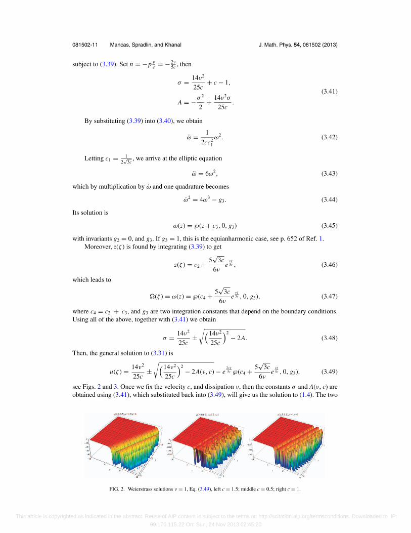
see Figs. 2 and 3. Once we fix the velocity c, and dissipation ν, then the constants σ and A(ν, c) areobtained using (3.41), which substituted back into (3.49), will give us the solution to (1.4). The two

FIG. 2. Weierstrass solutions ν = 1, Eq. (3.49), left c = 1.5; middle c = 0.5; right c = 1.

This article is copyrighted as indicated in the abstract. Reuse of AIP content is subject to the terms at: http://scitation.aip.org/termsconditions. Downloaded to IP:

99.170.115.22 On: Sun, 24 Nov 2013 02:45:20

081502-12 Mancas, Spradlin, and Khanal J. Math. Phys. 54, 081502 (2013)

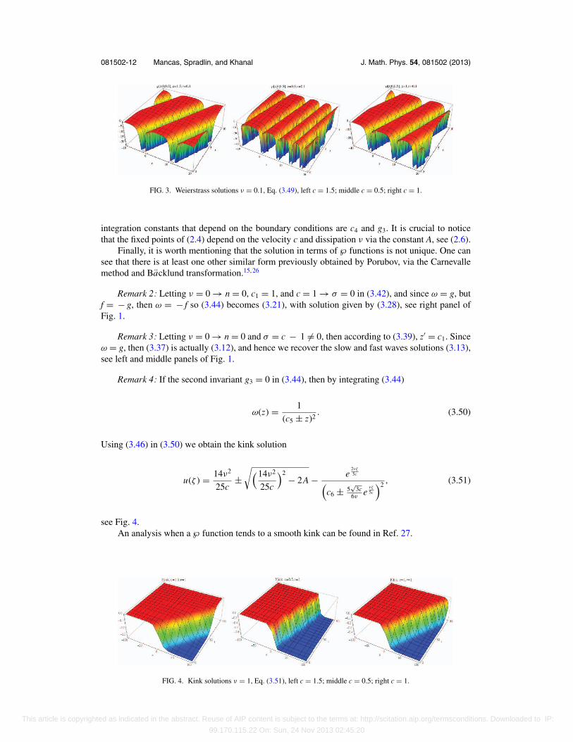
FIG. 3. Weierstrass solutions ν = 0.1, Eq. (3.49), left c = 1.5; middle c = 0.5; right c = 1.

integration constants that depend on the boundary conditions are c4 and g3. It is crucial to noticethat the fixed points of (2.4) depend on the velocity c and dissipation ν via the constant A, see (2.6).

Finally, it is worth mentioning that the solution in terms of ℘ functions is not unique. One cansee that there is at least one other similar form previously obtained by Porubov, via the Carnevallemethod and Backlund transformation.15, 26

Remark 2: Letting ν = 0 → n = 0, c1 = 1, and c = 1 → σ = 0 in (3.42), and since ω = g, butf = − g, then ω = − f so (3.44) becomes (3.21), with solution given by (3.28), see right panel ofFig. 1.

Remark 3: Letting ν = 0 → n = 0 and σ = c − 1 �= 0, then according to (3.39), z′ = c1. Sinceω = g, then (3.37) is actually (3.12), and hence we recover the slow and fast waves solutions (3.13),see left and middle panels of Fig. 1.

Remark 4: If the second invariant g3 = 0 in (3.44), then by integrating (3.44)

ω(z) = 1

(c5 ± z)2. (3.50)

Using (3.46) in (3.50) we obtain the kink solution

u(ζ ) = 14ν2

25c±

√(14ν2

25c

)2− 2A − e

2νζ

5c(c6 ± 5

√3c

6νe

νζ

5c

)2 , (3.51)

see Fig. 4.An analysis when a ℘ function tends to a smooth kink can be found in Ref. 27.

FIG. 4. Kink solutions ν = 1, Eq. (3.51), left c = 1.5; middle c = 0.5; right c = 1.

This article is copyrighted as indicated in the abstract. Reuse of AIP content is subject to the terms at: http://scitation.aip.org/termsconditions. Downloaded to IP:

99.170.115.22 On: Sun, 24 Nov 2013 02:45:20

081502-13 Mancas, Spradlin, and Khanal J. Math. Phys. 54, 081502 (2013)

FIG. 5. Phase-plane for c = 0.5, left ν = 1, (0.0) node, ( − 1, 0) saddle; right ν = 0.1, (0.0) spiral, ( − 1, 0) saddle.

Remark 5: If A = 0 → c − 1 = ±k = ± 14ν2

25c , and one selects the lower branch of the radical,we obtain

u(ζ ) = − e2νζ

5c ℘(c4 + 5

ν

√c

3ae

νζ

5c , 0, g3), if g3 �= 0,

u(ζ ) = − e2νζ

5c(c6 ± 5

√3c

6νe

νζ

5c

)2 , if g3 = 0.

(3.52)

IV. STABILITY OF THE VISCOUS WAVES

In this section we consider the two-mode dynamical system of (2.4) with equilibrium points inthe phase plane (φ, ψ) at (0, 0) and (c − 1 ±

√(c − 1)2 + 2A, 0), where A = A(ν, c) is obtained from

(3.41). All the equilibrium points lie only in the plane ψ = 0, in the (φ, ψ , c) space. The bifurcationcurves are given by φ

(φ − (c − 1) ∓

√(c − 1)2 + 2A

) = 0, which are two constant lines. Near theorigin (φ − , 0) = (0, 0) [

φ′

ψ ′

]=

[0 1

− 1−cc

νc

] [φ

ψ

]. (4.1)

Following standard methods of phase-plane analysis the characteristic polynomial of the Jacobianmatrix of (4.1) evaluated at the fixed point (φ − , 0) is

g0(λ) = λ2 − p0λ + q0 = 0, (4.2)

where p0 = νc and q0 = 1−c

c .Since ν > 0, c > 0, then p0 > 0, hence the origin is unstable. Also, putting � = p2

0 − 4q0 =ν2−4c(1−c)

c2 , we have the following cases:

(i) 0 < c < 1, gives q0 > 0. If ν > 2√

c(1 − c) > 0, the origin is unstable node; if 0 < ν <

2√

c(1 − c), the origin is unstable spiral, see Fig. 5 and(ii) c > 1, gives q0 < 0 ⇒ � > 0, hence the origin is a saddle point, see Fig. 6.

Near the secondary fixed point (φ+, 0) = (c − 1 ±√

(c − 1)2 + 2A, 0)[φ′

ψ ′

]=

[0 1

1−cc

νc

] [φ

ψ

]. (4.3)

FIG. 6. Phase-plane for c = 1.5, left ν = 1, (0.0) saddle, (1, 0) node; right ν = 0.1, (0.0) saddle, (1, 0) spiral.

This article is copyrighted as indicated in the abstract. Reuse of AIP content is subject to the terms at: http://scitation.aip.org/termsconditions. Downloaded to IP:

99.170.115.22 On: Sun, 24 Nov 2013 02:45:20

081502-14 Mancas, Spradlin, and Khanal J. Math. Phys. 54, 081502 (2013)

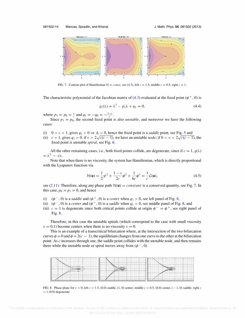
FIG. 7. Contour plot of Hamiltonian H = const , see (4.5), left c = 1.5; middle c = 0.5; right c = 1.

The characteristic polynomial of the Jacobian matrix of (4.3) evaluated at the fixed point (φ + , 0) is

g1(λ) = λ2 − p1λ + q1 = 0, (4.4)

where p1 = p0 = νc and q1 = −q0 = − 1−c

c .Since p1 = p0, the second fixed point is also unstable, and moreover we have the following

cases:

(i) 0 < c < 1, gives q1 < 0 ⇒ � > 0, hence the fixed point is a saddle point, see Fig. 5 and(ii) c > 1, gives q1 > 0. if ν > 2

√c(c − 1), we have an unstable node; if 0 < ν < 2

√c(c − 1), the

fixed point is unstable spiral, see Fig. 6.

All the other remaining cases, i.e., both fixed points collide, are degenerate, since if c = 1, g(λ)= λ2 − νλ.

Note that when there is no viscosity, the system has Hamiltonian, which is directly proportionalwith the Lyapunov function via

H(u) = 1

2ψ2 + 1 − c

2cφ2 + 1

6cφ3 = 1

cL(u), (4.5)

see (2.11). Therefore, along any phase path H(u) = constant is a conserved quantity, see Fig. 7. Inthis case, p0 = p1 = 0, and hence

(i) (φ − , 0) is a saddle and (φ + , 0) is a center when q1 > 0, see left panel of Fig. 8,(ii) (φ − , 0) is a center and (φ + , 0) is a saddle when q1 < 0, see middle panel of Fig. 8, and(iii) c = 1 is degenerate since both critical points collide at origin φ − = φ + , see right panel of

Fig. 8.

Therefore, in this case the unstable spirals (which correspond to the case with small viscosityν = 0.1) become centers when there is no viscosity ν = 0.

This is an example of a transcritical bifurcation where, at the intersection of the two bifurcationcurves φ = 0 and φ = 2(c − 1), the equilibrium changes from one curve to the other at the bifurcationpoint. As c increases through one, the saddle point collides with the unstable node, and then remainsthere while the unstable node or spiral moves away from (φ − , 0).

FIG. 8. Phase-plane for ν = 0, left c = 1.5, (0.0) saddle, (1, 0) center; middle c = 0.5, (0.0) center, ( − 1, 0) saddle; right c= 1 (0.0) degenerate.

This article is copyrighted as indicated in the abstract. Reuse of AIP content is subject to the terms at: http://scitation.aip.org/termsconditions. Downloaded to IP:

99.170.115.22 On: Sun, 24 Nov 2013 02:45:20

081502-15 Mancas, Spradlin, and Khanal J. Math. Phys. 54, 081502 (2013)

V. SUMMARY

In this paper a basic theory for the BBM equation (1.3), and its extension (1.4) to include thedissipation term was shown. When the viscous term is not present, (1.3) has traveling wave solutionsthat depend critically on the traveling wave velocity. When the velocity c > 1 (1.4) has solitary wavessolutions, while if c < 1, the solutions become periodic. At the interface between the two cases,when c = 1, the solutions are rational functions of cnoidal waves. Based on Ince’s transformation, atheory including the dissipative term was presented, in which we have found more general solutionsin terms of Weierstrass elliptic ℘ functions. Using dynamical systems theory we have shown thatthe solutions of (1.4) experience a transcritical bifurcation when c = 1, where at the intersection ofthe two bifurcation curves, stable equilibrium changes from one curve to the other at the bifurcationpoint. As the velocity changes, the saddle point collides with the node at the origin, and then remainsthere, while the stable node moves away from the origin. Also, the bifurcation curves and thefixed points of the dynamical system are functions of the traveling wave velocity c and dissipationconstant ν.

1 M. Abramowitz and I. Stegun, Handbook of Mathematical Functions: With Formulas, Graphs, and Mathematical Tables(Dover, NY, 1972).

2 C. J. Amick, J. L. Bona, and M. Schonbek, “Decay of solutions of some nonlinear wave equations,” J. Differ. Equations81, 1–49 (1989).

3 M. Arias, J. Campos, A. M. Robles-Perez, and L. Sanchez, “Fast and heteroclinic solutions for a second order ODE relatedto Fisher-Kolmogorov’s equation,” Calculus Var. Partial Differ. Equ. 21(3), 319–334 (2004).

4 C. Baesens and R. S. MacKay, “Uniformly travelling water waves from a dynamical systems viewpoint: some insights intobifurcations from Stokes’ family,” J. Fluid Mech. 241, 333–347 (1992).

5 T. B. Benjamin, J. L. Bona, and J. J. Mahony, “Model equations for long waves in nonlinear dispersive systems,” Philos.Trans. R. Soc. London, Ser. A 272(1220), 47–78 (1972).

6 T. B. Benjamin, “The stability of solitary waves,” Proc. R. Soc. London, Ser. A 328, 153–183 (1972).7 M. L. Bertotti and P. Montecchiari, “Connecting orbits for some classes of almost periodic Lagrangian systems,” J. Differ.

Equations 145(2), 453–468 (1998).8 J. L. Bona and T. Nikolay, “Sharp well-posedness results for the BBM equation,” Discrete Contin. Dyn. Syst 23, 1241–1252

(2009).9 J. L. Bona, W. G. Pritchard, and L. R. Scott, “An evaluation of a model equation for water waves,” Philos. Trans. R. Soc.

London, Series A, Math. Phys. Sci. 302(1471), 457–510 (1981).10 F. Bowman, Introduction of Elliptic Functions with Applications (Dover, NY, 1961).11 P. F. Byrd and M. D. Friedmann, Hanbook of Elliptic Integrals for Engineers and Scientists (Springer-Verlag, NY, 1971).12 A. Choudhuri, B. Talukdar, and U. Das, “Dynamical systems theory for nonlinear evolution equations,” Phys. Rev. E 82(3),

036609 (2010).13 E. L. Ince, Ordinary Differential Equations (Dover, NY, 1926).14 D. J. Korteweg and G. de Vries, “On the change of form of long waves advancing in a rectangular canal, and on a new

type of long stationary waves,” Phil. Mag. 39(5), 422–443 (1895), courtesy of Bijzondere Collecties, Universiteit vanAmsterdam, plaatsnummer UBM: DT 9721.

15 N. A. Kudryashov, “On “new travelling wave solutions” of the KdV and the KdV-Burgers equations,” Commun. NonlinearSci. Numer. Simul. 14(5), 1891–1900 (2009).

16 D. W. Jordan and P. Smith, Nonlinear Ordinary Differential Equations (An Introduction to Dynamical Systems) (OxfordUniversity Press, 1999).

17 H. Lemke, Sitzungsberichte der Berliner Math. Ges. 18, 26–31 (1920), ordered via library loan from Indiana UniversityILL:98768894.

18 S. C. Mancas and H. C. Rosu, “Integrable dissipative nonlinear second order differential equations via factorizations andAbel equations,” Phys. Lett. A 377(21–22), 1434–1438 (2013).

19 J. Nickel, “Elliptic solutions to a generalized BBM equation,” Phys. Lett. A 364, 221–226 (2007).20 P. Painleve, “Sur les lignes singulieres des fonctions analitiques,” Premiere theses (Academie de Paris, 1887).21 D. H. Peregrine, “Calculations of the development of an undular bore,” J. Fluid Mech. 25, 321 (1966).22 D. H. Peregrine, “Long waves on a beach,” J. Fluid Mech. 27, 815–827 (1967).23 D. H. Peregrine, “Water waves and their development in space and time,” Proc. R. Soc. London, Ser. A 400, 1–18 (1985).24 O. Cornejo-Perez and H. C. Rosu, “Solutions of the perturbed KdV equation for convecting fluids by factorizations,” Cent.

Eur. J. Phys. 8(4), 523–526 (2010).25 H. Poincare, “Sur une theorem de M. Fuchs,” Acta Math. 7, 1–32 (1885).26 A. V. Porubov, “Exact travelling wave solutions of nonlinear evolution equation of surface waves in a convective fluid,” J.

Phys. A 26, L797–L800 (1993).27 A. Samsonov, “Travelling wave solutions for nonlinear dispersive equations with dissipation,” Appl. Anal. 57, 85–100

(1995).

This article is copyrighted as indicated in the abstract. Reuse of AIP content is subject to the terms at: http://scitation.aip.org/termsconditions. Downloaded to IP:

99.170.115.22 On: Sun, 24 Nov 2013 02:45:20