WEIERSTASS-LIKE METHODS WITH CORRECTIONSFOR THE INCLUSION OF POLYNOMIAL ZEROS

L. D. Petkovic∗1, M. S. Petkovic∗∗ and D. Milosevic∗∗∗ Faculty of Mechanical Engineering, University of Nis, 18 000 Nis, Serbia and Montenegro∗∗ Faculty of Electronic Engineering, University of Nis, 18 000 Nis, Serbia and Montenegro

Abstract. In this paper we present iteration methods of Weierstrass’ type for the simultaneous inclusion

of all (simple or multiple) zeros of a polynomial. The main advantage of the proposed methods consists

of the increase of the convergence rate applying correction terms. Using the concept of the R-order of

convergence of mutually dependent sequences, we present the convergence analysis for the total-step and

the single-step methods. Numerical examples are given.

Key words: Zeros of polynomials, simultaneous methods, convergence rate, circular arithmetic.

AMS(MOS) subject classification: 65H05

1. Introduction

Iterative methods for the simultaneous determination of complex zeros of a given polynomial,realized in complex interval arithmetic, are a new and very efficient device to error estimates for agiven set of approximate zeros. After the fundamental paper [7] of Gargantini and Henrici in 1972,a number of methods for the simultaneous inclusion of polynomial zeros was constructed. Moredetails about this type of methods, including studies on convergence properties, computationalefficiency, numerical experiments and parallel implementation, can be found in the books [11]and [15] and references cited there. In general, inclusion methods, realized in complex intervalarithmetic, produce resulting disks or rectangles containing complex zeros. In this manner, theupper error bounds, given by the radii of disks or the semidiagonals of rectangles, are obtainedautomatically. This very fruitful property of self-validated results, together with the ability toincorporate rounding errors without altering the fundamental structure of the iterative formula,led to frequent application of inclusion methods for solving many problems which appear not onlyin applied mathematics but also in mathematical models in physics and engineering sciences.A significant improvement of computational efficiency of simultaneous inclusion methods was

gained by using suitable correction terms. Such an approach, based on Nourein’s idea [8] for thesimultaneous methods in ordinary complex arithmetic, was applied for the first time in [13] to theBorsch-Supan method. This idea was later applied to the Aberth-Ehrlich method [3] and the Halleymethod [12]. The aim of this paper is to present in details iterative methods of Weierstrass’ typefor the simultaneous inclusion of the zeros of a polynomial where the improved convergence orderis attained by using convenient corrections.Consider a monic polynomial of degree n ≥ 3

P (z) = zn + an−1zn−1 + · · ·+ a1z + a0 =

n∏j=1

(z − ζj) (aj ∈ C) (1)

1Correspondence: e-mail: ljiljana@masfak.ni.ac.yu

1

2

with simple complex zeros ζ1, ..., ζn. Hence we obtain the fixed point relations

ζk = z − P (z)n∏

j=1j =k

(z − ζj)

(k = 1, ..., n). (2)

Assume that distinct complex numbers z1, ..., zn are reasonably good approximations to the zerosζ1, ..., ζn of P. Putting z = zk and substituting the zeros ζj by their approximations zj (j = k) in(2), we obtain the well known Weierstrass iterative method (known also as Dochev-Durand-Kernermethod, see [4,7,18])

zk = zk − P (zk)n∏

j=1j =k

(zk − zj)

(k = 1, ..., n). (3)

Here zk is a new approximation to the zero ζk. Docev [4] was the first who proved the quadraticconvergence of this algorithm.Let us introduce the abbreviations

Nk =P (zk)P ′(zk)

(Newton’s correction), Wk =P (zk)

n∏j=1j =k

(zk − zj)

(Weierstrass’ correction).

Then, starting from the iterative formula (3), Nourein [8] has constructed the modified Weierstrass’method

zk = zk − P (zk)n∏

j=1j =k

(zk − zj +Wj)

(k = 1, ..., n). (4)

The order of convergence of the method (4) is three. The same improvement is attained usingNewton’s correction, that is, we can also formulate the modified cubically convergent method

zk = zk − P (zk)n∏

j=1j =k

(zk − zj +Nj)

(k = 1, ..., n). (5)

Both methods (4) and (5) require the same number of numerical operations so that their compu-tational efficiency is the same.Starting from the fixed point relation (2) and disjoint initial intervals Z(0)

1 , ..., Z(0)n (real intervals,

disks or rectangles) which contain the zeros ζ1, ..., ζn respectively, Alefeld and Herzberger [2, Ch.8]constructed the interval version of Weierstrass’ formula in the form

Z(m+1)k = z

(m)k − P (z(m)

k )n∏

j=1j =k

(z(m)k − Z

(m)j

) (k = 1, ..., n; m = 0, 1, ...), (6)

3

where z(m)k is the center of the interval Z(m)

k . The main advantage of the interval method (6) isthat ζk ∈ Z

(m)k for all k = 1, ..., n and m = 1, 2, ..., which provides the upper error bounds of

approximations (given by the semiwidths, radii or semidiagonals).As in [11, Ch.3] and [17] we will develop our algorithms in complex circular arithmetic. For

m = 0, 1, 2, . . . let us introduce the abbreviations

Z(m)k =

z(m)k ; r(m)

k

, r(m) = max

1≤k≤nr(m)k , ρ(m) = min

k,jk =j

|z(m)k − z

(m)j | − r

(m)j ,

where z(m)k is the center of the disk Z

(m)k and r

(m)k is its radius. Following the same technique and

derivation presented in [11, Ch. 3] we can state

Theorem 1. Under the conditionρ(0) >

72(n− 1)r(0),

the iteration method (6) converges quadratically, and for each k = 1, ..., n and m = 0, 1, ... thefollowing is valid:

(i) ρ(m) > 72 (n− 1)r(m); (7)

(ii) ζk ∈ Z(m)k .

Considering the iterative formulas (4) and (5) the following natural question arises: is it possibleto increase the convergence rate of Weierstrass-like interval method (6) using the corrections Nk

or Wk ? The study of this problem is the aim of this paper.

2. Circular complex arithmetic

Development and convergence analysis of the proposed algorithms need the basic propertiesof the so-called circular complex arithmetic introduced by Gargantini and Henrici [5]. A circularclosed region (disk) Z := z : |z − c| ≤ r with center c := midZ and radius r := radZ we willdenote by parametric notation Z := c; r. If Zk := ck; rk (k = 1, 2), then

Z1 ± Z2 = c1 ± c2; r1 + r2,Z1 · Z2 = c1c2; |c1|r2 + |c2|r1 + r1r2,

Z−1 = c; r−1 =c; r

|c|2 − r2(|c| > r, i.e. 0 /∈ Z),

Z1 : Z2 = Z1 · Z−12 (0 /∈ Z2).

We will also use the inversion in the centered form:

ZI := c; rI =1c;

r

|c|(|c| − r)

(|c| > r, i.e. 0 /∈ Z).

Let us note thatc; r−1 ⊂ c; rI . (8)

In the sequel, INV (Z) will denote one of the two inversions Z−1 or ZI .For the basic interval operations +,−, ·, : the inclusion property is valid, that is,

Zk ⊆ Wk ⇒ Z1 ∗ Z2 ⊆ W1 ∗W2 (k = 1, 2; ∗ ∈ +,−, ·, :).

4

Moreover, if f is a rational function and F its complex circular extension, then

Zk ⊆ Wk (k = 1, . . . , q)⇒ F (Z1, . . . , Zq) ⊆ F (W1, . . . ,Wq).

Particularly, we have

wk ∈ Wk (k = 1, . . . , q; wk ∈ C)⇒ f(w1, . . . , wq) ∈ F (W1, . . . ,Wq).

In this paper we will use the following obvious implications:

z ∈ c; r ⇔ |z − c| ≤ r. (9)

z /∈ c; r ⇔ |z − c| > r. (10)

For a disk Z = c; r which does not contain the origin (that is, |c| > r), the k-th root of Z isdefined by the union (see [10])

Z1/k :=k−1⋃λ=0

|c|1/k exp

(arg c+ 2λπk

i); |c|1/k − (|c| − r)1/k

. (11)

More details about circular arithmetic can be found in the books [2, Ch.5] and [15, Ch.1].Throughout this paper disks in the complex plane will be denoted by capital letters.

3. Inclusion methods with corrections: simple zeros

Further increase of the convergence speed of the iteration methods (4) and (5) can be achieved us-ing Newton’s correction N(zk) = P (zk)/P ′(zk) or Weierstrass’ correction Wk = P (zk)/

∏j =k(zk −

zj) in the similar way as in [3] and [13]. In this construction we assume the choice of initial inclusiondisks satisfying the condition (7), which provides the convergence of the iteration methods (4) and(5) (see Theorem 1). For simplicity, we will omit the iteration index m and write, for example,

zk, zk, rk, rk, r, r, Zk, Zk, ρ, ρ

instead ofz(m)k , z

(m+1)k , r

(m)k , r

(m+1)k , r(m), r(m+1), Z

(m)k , Z

(m+1)k , ρ(m), ρ(m+1).

Lemma 1. Let εj := zj − ζj (j = 1, . . . , n). For Weierstrass’ corrections Wj the following is valid:

(i) |Wj | ≤ |εj |(1 +

r

ρ

)n−1

;

(ii) |zj −Wj − ζj | ≤ |εj |[(1 +

r

ρ

)n−1

− 1].

The proof of the above inequalities is similar to that presented in [13].

Lemma 2. Let Z1, ..., Zn be inclusion disks for the zeros ζ1, ..., ζn, ζk ∈ Zk, and let zk =midZk, rk = radZk, εk = zk − ζk. If the inclusion disks Z1, ..., Zn are chosen so that the in-equality

ρ >72(n− 1)r (12)

is satisfied, then for all k = 1, . . . , n we have

5

(i) ζk ∈ Zk ⇒ ζk ∈ ZW,k := Zk −W (zk);(ii) 0 /∈ HW,k :=

∏j =k(zk − ZW,j);

(iii) ζk ∈ Zk ⇒ ζk ∈ ZN,k := Zk −N(zk);(iv) 0 /∈ HN,k :=

∏j =k(zk − ZN,j).

Proof. Of (i): It is sufficient to prove the implication

|zk − ζk| = |εk| ≤ rk ⇒ |zk −Wk − ζk| ≤ rk.

According to (12) and the assertion (ii) of Lemma 1 we have

|zk −Wk − ζk| < |εk|[(1 +

27(n − 1)

)n−1

− 1]< |εk|(e2/7 − 1) < 1

3|εk| < rk.

Of (ii): Let ykj = rj/|zk − zj +Wj |. Since

HW,k =∏j =k

(zk − Zj +Wj) =∏j =k

(zk − zj +Wj) ·1;

∏j =k

(1 + ykj)− 1,

having in mind the implication

0 /∈ HW,k ⇔ 1 >∏j =k

(1 + ykj)− 1,

we have to prove the inequality∏

j =k(1 + ykj) < 2.In view of (i) of Lemma 1 we have by (12)

|Wj | < |εj |(1 +

27(n − 1)

)n−1

< e2/7|εj | < 43r,

so that|zk − zj +Wj | ≥ |zk − zj | − |Wj | > ρ+ rj − 4

3rj > ρ− 1

3r > ρ− 2

5r.

Therefore, ykj <r

ρ− 2r/5 and hence, by (12),

∏j =k

(1 + ykj) <(1 +

r

ρ− 2r/5)n−1(

1 +1

7(n− 1)/2 − 2/5)n−1

< e2/7 < 2. (13)

Of (iii): According to (i) we should prove the implication

|zk − ζi| < rk ⇒ |zk −N(zk)− ζk| < rk.

Since|zk − ζj | > |zk − zj | − |zj − ζj | > |zk − zj | − rj ≥ ρ,

we findσk :=

∣∣∣∑j =k

(zk − ζj)−1∣∣∣ ≤ ∑

j =k

|zk − ζj |−1 <n− 1ρ

.

6

By virtue of this and (12) we obtain

rk <2ρ

7(n − 1) <27σk

,

wherefrom there followsrkσk

1− rkσk<25.

Since1Nk

=P ′(zk)P (zk)

=n∑

j=1

(zk − ζj)−1 = 1/εk +∑j =k

(zk − ζj)−1,

using the last inequality and |εk| = |zk − ζk| < rk we get

|zk −N(zk)− ζk| = |εk −N(zk)| = |εk|2∣∣∣ σk

1 + εkσk

∣∣∣ < rkrkσk

1− rkσk<25rk < rk.

Of (iv): First we have

HN,k =∏j =k

(zk − Zj +Nj) =∏j =k

(zk − zj +Nj) ·1;

∏j =k

(1 + xkj)− 1,

where xkj = rj/|zk − zj +Nj |. Using (12) we obtain the estimate

1|Nk| =

∣∣∣∣∣∣1

zk − ζk+

∑j =k

1zk − ζj

∣∣∣∣∣∣ >1

|zk − ζk| −∑j =k

1|zk − ζj |

>1rk

− n− 1ρ

>1rk

− 2(n − 1)7(n − 1)rk

=57rk

,

whence |Nk| < 57rk. According to this we get

|zk − zj +Nj | > |zk − zj | − |Nj | > ρ+ rj − 75rj > ρ− 2

5r,

so that xkj < r/(ρ− 2r/5). Hence, by (12),∏j =k

(1 + xkj) <(1 +

r

ρ− 2r/5)n−1

<(1 +

17(n− 1)/2 − 2/5

)n−1

< e2/7 < 2. (14)

But, as in the proof of (ii), the last inequality provides that 0 /∈ HN,k. Starting from the iterative formulas (5) and (4) we can construct modified Weierstrass inclusion

methods for simple zeros in the form

Zk = zk − P (zk) · INV

(n∏

j=1j =k

(zk − Zj +Nj)

)(k = 1, ..., n), (15)

Zk = zk − P (zk) · INV

(n∏

j=1j =k

(zk − Zj +Wj)

)(k = 1, ..., n). (16)

7

where INV in (15) and (16) denotes inversions of a disk defined in Section 1, that is, INV ∈()−1, ()I. As mentioned above, these formulas will define inclusion methods only if ζj ∈ Zj −Wj ∧ 0 /∈ HW,k and ζj ∈ Zj −Nj ∧ 0 /∈ HN,k, respectively. These conditions are considered inLemma 2, which means that if (12) holds, then ζk ∈ Zk for each k = 1, ..., n.Let us define

uk =∏j =k

(zk − zj +Nj), vk =∏j =k

(zk − zj +Wj), q =r

ρ− 2r/5 .

Then the following is valid:

Lemma 3. Let (12) be satisfied. Then

HN,k =∏j =k

(zk − Zj +Nj) ⊂ uk

1;13

, (17)

HW,k =∏j =k

(zk − Zj +Wj) ⊂ vk

1;13

. (18)

Proof. First, we have

HN,k =∏j =k

(zk − zj +Nj) ·1;

∏j =k

(1 +

rj

|zk − zj +Nj |)− 1

= uk

1;

∏j =k

(1 + xkj)− 1.

Using (14) we findHN,k ⊂ uk

1; (1 + q)n−1 − 1

. (19)

Sinceq =

1ρ/r − 2/5 <

17(n − 1)/2 − 2/5 ,

we estimate(1 + q)n−1 − 1 <

(1 +

17(n − 1)/2 − 2/5

)n−1

− 1 < e2/7 − 1 < 13,

and from (19) we immediately obtain the inclusion (17).Using the inequality (13), in a quite similar way we obtain

HW,k ⊂ vk

1; (1 + q)n−1 − 1

⊂ vk

1;13

. (20)

Hence the inclusion (15) follows. The order of convergence of the inclusion methods (15) and (16) with corrections is considered

in the following theorem:

Theorem 2. Let (Z1, ..., Zn) := (Z(0)1 , ..., Z

(0)n ) be initial disks such that ζk ∈ Zk (k = 1, ..., n) and

let (Z(m)k ) (k = 1, ..., n) denote the sequences of disks produced by (15) or (16), where m = 0, 1, 2, ...

is the iteration index. If the condition

ρ(0) >72(n− 1)r(0) (21)

8

holds, then for any k ∈ 1, ..., n and m = 0, 1, ... there holds ζk ∈ Z(m)k and the sequences of radii

(r(m)k ) (k = 1, ..., n) tend monotonically towards 0.

Proof. Theorem 2 will be proved by induction on m. First, let m = 0. We will analyze theiteration formula (15) with Newton’s correction. This formula can be written in the form

Zk = zk − P (zk)INV (HN,k) ⊆ zk − P (zk)[HN,i]I

due to (8). Hence, according to Lemma 3, we obtain

Zk ⊆ zk − P (zk)uk

1;13

I

= zk − P (zk)uk

1;12

. (22)

Furthermore, in regard to the proof of Lemma 2 (the assertions (iii) and (iv)), we estimate

|zj −Nj − ζj ||zk − zj +Nj | <

2r/5ρ− 2r/5

so that∣∣∣∣P (zk)

uk

∣∣∣∣ = |zk − ζk|∣∣∣∣∣∣∏j =k

zk − ζj

zk − zj +Nj

∣∣∣∣∣∣ ≤ |εk|∏j =k

(1 +

∣∣∣zj −Nj − ζk

zk − zj +Nj

∣∣∣)

< |εk|∏j =k

(1 +25q) < rk(1 +

25q)n−1 < e4/35rk <

65rk.

According to the last inequality and the inclusion (22) we find

rk ≤∣∣∣∣P (zk)

uk

∣∣∣∣ rad1; 12< ω rk. (23)

where we setω =

35.

Since ζj ∈ Zj (j = 1, ..., n), according to the inclusion property from the fixed point relation (2)and the iteration formula (15) it follows ζk ∈ Zk. Using this fact and (23) we have

|zk − ζk| < rk < ω rk.

Since ζk ∈ Zk, that is, |zk − ζk| < rk, we get

|zk − zk| < |zk − ζk|+ |zk − ζk| < rk + rk < (1 + ω)rk.

According to this and (23) we estimate for any pair k, j ∈ 1, . . . , n (k = j)

|zk − zj | − rj ≥ |zk − zj | − |zj − zj | − |zk − zk| − rj

> ρ+ rj − (1 + ω)rj − (1 + ω)rk − ω rj ≥ ρ− (3ω + 1)r,which means that ρ > ρ− (3ω + 1)r. In regard to the last inequality and (12) we find

r

ρ<

ω r

ρ− (3ω + 1)r =r

ρ· ω

1− (3ω + 1) rρ

<r

ρ· ω

1− 2(3ω + 1)7(n − 1)

≤ r

ρ· ω

1− (3ω + 1)/7 =r

ρ· 7ω6− 3ω =

r

ρ<

27(n − 1) .

9

Hence, we conclude by induction that the initial condition (21) implies the inequality ρ(m) >72(n − 1)r(m) for each m = 0, 1, ... . Therefore, the assertions of Lemma 2 and 3 hold for each

m = 0, 1, ... .First, by virtue of Lemma 2 we have ζk ∈ Z

(m)k −N(z(m)

k ) for any k ∈ 1, ..., n. According tothis and the inclusion property from (12) we obtain ζk ∈ Z

(m+1)k . Since ζj ∈ Z

(0)j , by induction

there follows ζk ∈ Z(m)k for each k ∈ 1, ..., n andm = 0, 1, 2, ... . Second, we see that the inversions

in (15) are defined in each iterative step which means that the inclusion methods (15) are feasible.Besides, the disks Z(m)

1 , ..., Z(m)n are nonintersecting since ρ(m) > 2r(m).

Finally, from the inequality (23) we conclude that the sequences of radii r(m)k (k = 1, ..., n)

converge monotonically towards 0.In a quite similar way we prove Theorem 2 for the inclusion method (16) with Weierstrass’

corrections. In order to determine the R−order of convergence, we will give a qualitative analysis of the

behavior of the centers and radii of the disks Z(m)1 , ..., Z

(m)n produced by the iteration formulas (15)

or (16), similar to that presented in the papers [3,12,13]. For this purpose we introduce for anym = 0, 1, ...

ε(m)k := z

(m)k − ζk, εm := max

k=1,...,n|ε(m)

k |, rm := maxk=1,...,n

r(m)k = r(m).

Lemma 4. Let β be equal 1 if INV = ()−1 and 0 if INV = ()I . Then for the inclusion methods(15) and (16) we have

(i) rm+1 = O(εmrm);(ii) εm+1 = O(ε3

m) + βO(εmr2m),

where O denotes the Landau symbol.

Proof. For simplicity, we will omit the iteration index and use the notations introduced previ-ously. Again, we will present the convergence analysis in the case of the iteration method (15) withNewton’s corrections. A quite similar analysis can be performed for the method (16).Newton’s method zk = zk −Nk has a quadratic convergence so we have

εk = zk − ζk = zk −Nk − ζk = O(ε2k).

Hence, there is a complex constant αk such that

P (zk)uk

= εk

∏j =k

zk − ζj

zk − zj +Nj= εk

∏j =k

(1 +

zj −Nj − ζj

zk − zj +Nj

)= εk

(1 + αkε

2 +O(ε4)).

Let τn = e2/7(n−1). Since q = r/(ρ− 2r/5) < 1/(7(n − 1)/2 − 2/5), we have

(1 + q)k <

[(1 +

17(n− 1)/2 − 2/5

)n−1]2k/7(n−1)

< e2k/7(n−1) = τkn (k = 1, . . . , n− 2),

so that

1 + (1 + q) + · · ·+ (1 + q)n−2 < 1 + τ + · · ·+ τn−2 <τn−1 − 1τ − 1

=e2/7 − 1

e2/7(n−1) − 1 <143(n− 1) =: ηn.

10

Here we used the inequality ex > 1 + x for x = 2/(7(n − 1)). Now, we estimate

(1 + q)n−1 − 1 = q(1 + (1 + q) + · · ·+ (1 + q)n−2

)< ηnq.

First, let us consider the inversion INV = ()−1 in (15), that is, let β = 1. We have foundpreviously the inclusion

Zk ⊂ zk − P (zk)uk

1; ηnq−1 = zk − P (zk)uk

· 1; ηnq1− (ηnq)2

. (24)

Hence

rk = radZk ≤ |εk|∏j =k

∣∣∣∣ zk − ζj

zk − zj +Nj

∣∣∣∣ · ηnq

1− (ηnq)2.

Since the product on the right-hand side is bounded and ηnq = O(r), we have

r = O(εr). (25)

For the center of the improved disk we have zk∼= zk − P (zk)

uk· 11− (ηnq)2

so that

εk = zk − ζk∼= εk − εk

1− (ηnq)2∏j =k

zk − ζj

zk − zj +Nj

= εk − εk

(1 + αkε

2 +O(ε4))(1 + (ηnq)2 + (ηnq)4 + · · · )

= εk − εk

(1 + α∗ε2 + β∗r2 +O(r2ε2)

),

wherefromεk = O(ε3) +O(εr2). (26)

Now, let us consider the inversion INV = ()I (β = 0). From (24) we obtain

Zk ⊂ P (zk)uk

1; ηnqI = zk − P (zk)uk

1;

ηnq

1− ηnq

.

Thereforer = O(εr) (27)

since P (zk)/uk = O(εk) and ηnq = O(r). Besides,

εk∼= εk − P (zk)

uk= εk − εk

(1 + αkε

2 +O(ε4))= O(ε3). (28)

The relations (25), (26), (27) and (28) proves (i) and (ii) in the case of the iteration method (15).As mentioned above, a similar proof can be given for the method (16). In Lemma 4 we have the case of two mutually dependent sequences. In order to determine their

order of convergence, we use the following special case of Theorem 4 presented in [6]:

Theorem 3. Given the error-recursion

ε(m+1)i ≤ αi

k∏j=1

(ε(m)j

)pij , (i = 1, . . . , k; m ≥ 0),

11

where pij ≥ 0, αi > 0, 1 ≤ i, j ≤ k. Denote the matrix of exponents with P, that is P = [pij ]k×k. Ifthe non-negative matrix P has the spectral radius ρ(P ) > 1 and a corresponding eigenvector x > 0,then the R-order of all sequences ε(m)

i (i = 1, . . . , k) is bounded below by the spectral radius ρ(P ).

In the sequel the matrix Pk = [pij ] will be called the R-matrix.

Let OR(IM) denote the R-order of convergence of an iteration method IM. Now we can givethe convergence theorem for the inclusion methods (15) and (16).

Theorem 4. Let OR(15) and OR(16) denote the R-order of the iteration interval methods (15)and (16) respectively, where INV ∈ ()−1, ()I. Then

OR(15) = OR(16) ≥1 +

√2 ∼= 2.414 if INV = ()−1,

3 if INV = ()I ,

Proof. Let us assume that |ε(0)| ≈ r(0) and |ε(m)| ≤ r(m) for m ≥ 1. We will distinguish twocases:

1) INV = ()−1, that is β = 1.

From Lemma 4 we haveεm+1 ∼ εmr2

m, rm+1 ∼ εmrm.

From these relations we form the R-matrix P(β=1)2 =

[1 21 1

]with the spectral radius ρ(P (β=1)

2 ) =

1 +√2 and the corresponding eigenvector xρ = (

√2, 1) > 0. Therefore, according to Theorem 3,

we obtain OR(12) = OR(13) ≥ ρ(P (β=1)2 ) = 1 +

√2 ∼= 2.414.

2) INV = ()I , that is β = 0. From Lemma 4 we form the relations

εm+1 ∼ ε3m, rm+1 ∼ εmrm.

Hence, we construct the R-matrix P(β=0)2 =

[3 01 1

]with ρ(P (β=0)

2 ) = 3 and xρ = (2, 1) > 0 and,

in regard to Theorem 3, we obtain OR(12) = OR(13) ≥ ρ(P (β=0)2 ) = 3.

4. Single-step methods

The convergence speed of the second order interval method (6) can be accelerated by applyingthe Gauss-Seidel approach (single step mode). The single step version of (6) reads

Zk = zk − P (zk)INV

(∏j<k

(zk − Zj)∏j>k

(zk − Zj)

)(k = 1, ..., n). (29)

For the R-order of (26) it holds that

OR((29)) ≥ 1 + τn,

where τn ≥ 1 is the unique positive root of the polynomial equation τn − τ − 1 = 0 (see Alefeldand Herzberger [2, Ch. 8]).

12

In the similar way the considered inclusion methods of Weierstrass’ type with corrections canbe further accelerated using the Gauss-Seidel procedure. Starting from (15) and (16) we can statethe following single-step inclusion method

Zk = zk − P (zk) · INV

(∏j<k

(zk − Zj)∏j>k

(zk − Zj +Nj)

)(k = 1, ..., n) (30)

with Newton’s corrections, and

Zk = zk − P (zk) · INV

(∏j<k

(zk − Zj)∏j>k

(zk − Zj +Wj)

)(k = 1, ..., n) (31)

with Weierstrass’ corrections. Therefore we use the already calculated circular approximations inthe same iteration.Because of the very complicated mutual dependence of even 2n sequences of centers and radii

of produced disks, it is very difficult to find the R-order of convergence of these methods. Besides,the number of zeros n (= the polynomial degree for simple zeros) is involved as a parameter so thatwe use the denotation OR(IM,n) for the R-order. Since the sought value OR(IM,n) for a specificn is not of great practical importance and does not deserve such a big effort, we will restrict ourattention to the determination of the bounds of the R-order taking the limit cases n = 2 and verylarge n.Let Ω, Ω(−1), ΩI be the ranges of the lower bounds of the R-order of convergence concerning

the inclusion single-step methods without corrections and with corrections using the inversions ()−1

and ()I , respectively.Having in mind the fact that the convergence rate of a considered single-step method becomes

almost the same as the one of the corresponding total-step method when the polynomial degree isvery large, according to Theorem 4 we have

OR(30) = OR(31) ≥1 +

√2 ∼= 2.414 if INV = ()−1,

3 if INV = ()I ,

for very large n.Consider now the single-step methods (30) and (31) for n = 2 and the inversion INV =

()−1 (β = 1).Without loss of generality we can assume that |ε(0)1 | = |ε(0)

2 | = r(0)1 = r

(0)2 (the ”worst

case” model). After an extensive calculation we derive the following estimates for both methods:

|ε1| ∼ |ε1|r22, |ε2| ∼ |ε1||ε2|r2

2, r1 ∼ |ε1|r2, r2 ∼ |ε1| |ε2|r2.

According to this we form the corresponding R-matrix

P(β=1)4 =

1 0 0 21 1 0 21 0 0 11 1 0 1

with ρ(P (β=1)4 ) = 3.214 and xρ = (1, 1.4517, 0.6556, 1.107) > 0. Now, in regard to Theorem 3, we

obtainOR((30), 2) = OR((31), 2) ≥ ρ(P (β=1)

4 ) = 3.214.

13

In the case of the inversion INV = ()I (β = 0) in the iteration formula (30) and (31), we canderive the following relations:

|ε1| ∼ |ε1||ε2|2, |ε2| ∼ |ε1||ε2|3, r1 ∼ |ε1|r2, r2 ∼ |ε1| |ε2|r2.

Hence we obtain the corresponding R-matrix

P(β=0)4 =

1 2 0 01 3 0 01 0 0 11 1 0 1

with ρ(P (β=0)4 ) = 3.732 and xρ = (1, 1.366, 0.5, 0.866) > 0. By Theorem 3 we find

OR((30), 2) = OR((31), 2) ≥ ρ(P (β=0)4 ) = 3.732.

According to the previous bounds for n = 2 and taking into account the results of Alefeld andHerzberger [1] for the Weierstrass’ single step method without corrections, we obtain the regions

Ω = (2, 2.618), Ω(−1) = (2.414, 3.214), ΩI = (3, 3.732).

5. Inclusion methods with corrections: multiple zeros

In this section we will consider Weierstrass-like method with corrections for the simultaneousinclusion of multiple zeros of a polynomial. Let

P (z) = zn + an−1zn−1 + · · ·+ a1z + a0 = (z − ζ1)µ1(z − ζ2)µ2 · · · (z − ζk)µν (32)

be a monic polynomial with multiple zeros ζ1, ..., ζν of the known multiplicities µ1, ..., µν , µ1+ · · ·+µν = n. From the factorization (32) we obtain the fixed point relations

ζk = z −[

P (z)∏j =k

(z − ζj)µj

]1/µk

∗(k = 1, ..., ν). (33)

The right-hand side in (33) will reduce to the zero ζk only for one particular determination of theµk−th root (µk > 1). The symbol ∗ indicates that only one (appropriate) of µk values of the µk−throot of a complex number has to be chosen.Let z1, . . . , zν be distinct approximations to the zeros ζ1, ..., ζν . Then the following iteration

formula for multiple zeros in ordinary complex arithmetic can be derived from (33) (see [16]):

zk = zk −[

P (zk)∏j =k

(zk − zj +Nj)µj

]1/µk

∗(k = 1, ..., ν). (34)

Newton’s correction Nj appearing in (34), often known as Shroeder’s correction, is given by Nj =µjP (zj)/P ′(zj). The order of convergence of the iteration method (34) is three. The proper valueof the µk−th root (which is indicated by ∗) should be selectd according to the criterion described

14

in [16]. In this section we will extended the iterative methods (33) and (34) to circular complexarithmetic.Assuming that ζk ∈ Zk, from the fixed point relation (33) we obtain

ζk ∈ zk − 1[1

P (zk)

∏j =k

(zk − Zj)µj

]1/µk

∗

(k = 1, ..., ν). (35)

Let Z1, . . . , Zν be disjoint disks containing the zeros ζ1, . . . , ζν respectively, and zk = mid Zk.According to (35) we can construct the following interval method of Weierstrass’ type for thesimultaneous inclusion of multiple zeros of a polynomial P :

Zk = zk − INV([ 1

P (zk)

∏j =k

(zk − Zj)µj

]1/µk

∗

)(k = 1, ..., ν). (36)

Let us now introduce the notations:

Nk = µkP (zk)P ′(zk)

,

Qk =1

P (zk)

∏j =k

(zk − zj +Nj)µk (k = 1, ..., ν).

Assuming that ζj ∈ ZN,j = zj −Nj , from the fixed point relation (33) we obtain

ζk ∈ zk − 1[1

P (zk)

∏j =k

(zk − Zj +Nj)µj

]1/µk

∗

= zk − 1[Qk

]1/µk

∗(k = 1, ..., ν). (37)

Let again Z1, . . . , Zν be disjoint disks containing the zeros ζ1, . . . , ζν respectively, and zk =mid Zk. According to (37) we can construct the following interval method of Weierstrass’ type withNewton’s corrections for the simultaneous inclusion of multiple zeros of a polynomial P :

Zk = zk − INV([ 1

P (zk)

∏j =k

(zk − Zj +Nj)µj

]1/µk

∗

)

= zk − INV([Qk

]1/µk

∗)(k = 1, ..., ν).

(38)

As in the case of Weierstrass’ method (34) in ordinary complex arithmetic, Schroeder’s cor-rection Nk = µjP (zk)/P ′(zk) is more convenient compared to Weierstrass’ correction Wk =[P (zk)/

∏j =k (zk − zj)

]1/µk since (the already calculated) Schroeder’s correction enables us toestablish an efficient criterion for the choice of the proper root-disk, referred to as CCR, amongµk (> 1) disks. Aside from this advantage, we note that Shroeder’s correction Nk is rather simplerfor calculation than Weierstrass’ correction Wk. If all zeros are simple, then both corrections givealgorithms (4) and (5) of the same computational costs.

Criterion for the root selection

First we are concerned here with the selection of the appropriate disk. The main idea hasbeen already presented in [16] in ordinary complex arithmetic so that we give only the outline of

15

CCR in complex circular arithmetic. Let µk > 1 and assume that disk Q1/µk

k does not containthe origin. Then Q

1/µk

k is the union of µk disjoint disks (see formula (11)), one of which contains

(zk − ζj)−1. Let that disk be denoted by[Qk

]1/µk

∗ = c∗k; d∗k. Denote the remaining µk − 1 disksQ

1/µk

k,λ , which do not contain (zk − ζj)−1, by ck,λ; dk, λ = 1, ..., µk − 1. Let us note that d∗k = dk

and ck,λ = c∗k exp(i2λπ

µk

), λ = 1, ..., µk − 1 adopting ck,0 = c∗k.

Let us introduce

ρ = mini =j

|zi − zj | − rj, r = rad1≤j≤s

rj , µ = min1≤k≤ν

µk, (39)

where zj = mid Zj , rj = rad Zj . The criterion for the choice of the appropriate disk[Qk

]1/µk

∗ isbased on the following assertion:

Lemma 5. If ρ > (n − 1)r and

dk <ρ− (n− µk)r

2µkρr,

then for each k = 1, . . . , ν it follows

(i) |N−1k − c∗k| ≤

n− µk

ρµk+ dk;

(ii) |N−1k − ck| ≥ n− µk

ρµk+ 3dk.

Proof. Using the logarithmic derivative we find

N−1k =

1µk

P ′(zj)P (zj)

=1µk

[ d

dzln

ν∏j=1

(z − ζj)µj

]z=zk

=1µk

ν∑j=1

µj

zk − ζj. (40)

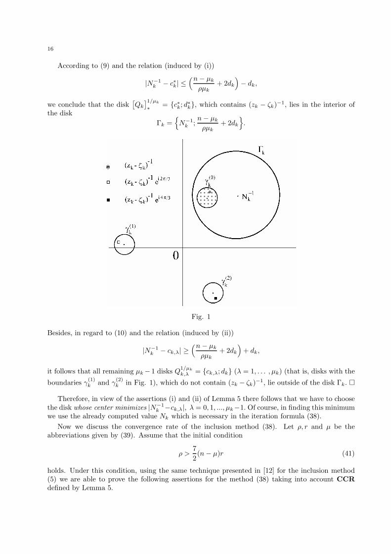
We will derive the proof of Lemma 5 using a geometric construction displayed in Fig. 1 (thecase µk = 3, where the boundaries of the disks

[Qk

]1/3

∗ = Q1/3k,0 , Q

1/3k,1 and Q

1/3k,2 are denoted by

γ(0)k , γ

(1)k , γ

(2)k , respectively).

Since N−1k − (zk − ζk)−1 ∈

N−1k − c∗k; d

∗k

, according to (40) we have

|N−1k − c∗k| ≤

∣∣∣ 1µk

s∑j=1

µj

zk − ζj− 1

zk − ζk

∣∣∣+ d∗k <n− µk

ρµk+ dk,

which proves (i).To prove (ii) we use (10) and the elementary inequality m sin π

m > 1 (m ≥ 2). We estimate forλ = 1, ..., µk − 1

|N−1k − ck,λ| ≥

∣∣∣ 1µk

ν∑j=1

µj

zk − ζj− 1

zk − ζkexp

(i2λπµk

)∣∣∣− dk

≥ 1|zk − ζk|

∣∣∣1− exp(i2λπµk

)∣∣∣− 1µk

∑j =k

µj

|zk − ζj | − dk ≥ 2rksin

λπ

µk− n− µk

ρµk− dk

≥ 2rµk

− n− µk

ρµk− dk =

2ρ− (n− µk)rrρµk

− 4dk + 3dk >n− µk

ρµk+ 3dk.

16

According to (9) and the relation (induced by (i))

|N−1k − c∗k| ≤

(n− µk

ρµk+ 2dk

)− dk,

we conclude that the disk[Qk

]1/µk

∗ = c∗k; d∗k, which contains (zk − ζk)−1, lies in the interior ofthe disk

Γk =N−1

k ;n− µk

ρµk+ 2dk

.

Fig. 1

Besides, in regard to (10) and the relation (induced by (ii))

|N−1k − ck,λ| ≥

(n− µk

ρµk+ 2dk

)+ dk,

it follows that all remaining µk − 1 disks Q1/µk

k,λ = ck,λ; dk (λ = 1, . . . , µk) (that is, disks with the

boundaries γ(1)k and γ

(2)k in Fig. 1), which do not contain (zk − ζk)−1, lie outside of the disk Γk.

Therefore, in view of the assertions (i) and (ii) of Lemma 5 there follows that we have to choosethe disk whose center minimizes |N−1

k −ck,λ|, λ = 0, 1, ..., µk−1. Of course, in finding this minimumwe use the already computed value Nk which is necessary in the iteration formula (38).Now we discuss the convergence rate of the inclusion method (38). Let ρ, r and µ be the

abbreviations given by (39). Assume that the initial condition

ρ >72(n− µ)r (41)

holds. Under this condition, using the same technique presented in [12] for the inclusion method(5) we are able to prove the following assertions for the method (38) taking into account CCRdefined by Lemma 5.

17

Lemma 6. Let Z1, ..., Zν be inclusion disks for the zeros ζ1, ..., ζν , ζk ∈ Zk, and let zk =midZk, rk = radZk, εk = zk − ζk. If the inclusion disks Z1, ..., Zν are chosen so that the in-equality (41) is satisfied, then we have for k = 1, . . . , ν :

(i) ζk ∈ Zk ⇒ ζk ∈ ZN,k := Zk −N(zk);

(ii) 0 /∈ HN,k :=∏

j =k(zk − ZN,k)µk .

Furthermore, introducing for any m = 0, 1, ... the quantities

ε(m)k := z

(m)k − ζk, εm := max

k=1,...,s|ε(m)

k |, rm := maxk=1,...,s

r(m)k = r(m),

we can prove

Lemma 7. Let β be equal 1 if INV = ()−1 and 0 if INV = ()I . Then for the inclusion method(38) we have

(i) rm+1 = O(εmrm);

(ii) εm+1 = O(ε3m) + βO(εmr2

m).

Lemma 6 gives conditions under which the inclusion method is defined, while Lemma 7 describesthe behaviour of the sequences of centers and radius of disks produced by (38). Using these lemmaswe establish the convergence theorem for the inclusion method (38):

Theorem 5. Let (Z1, ..., Zν) := (Z(0)1 , ..., Z

(0)ν ) be initial disks such that ζk ∈ Zk (k = 1, ..., ν) and

let Z(m)k (k = 1, ..., ν) denote the sequences of disks produced by (38), where m = 0, 1, ... is the

iteration index. If the condition

ρ(0) >72(n− µ)r(0)

holds, then for any k ∈ 1, ..., ν and m = 0, 1, ... there holds ζk ∈ Z(m)k and the sequences of radii

r(m)k (k = 1, ..., ν) tend monotonically towards 0.

Similar as in Section 4 (the case of simple zeros, see also [14]), we determine the convergencerate of the inclusion method (38) for multiple zeros:

Theorem 6. Let OR(10) denote the R-order of the iteration interval method (36), where INV ∈()−1, ()I. Then

OR(10) ≥1 +

√2 ∼= 2.414 if INV = ()−1,

3 if INV = ()I .

6. Numerical examples

In this section we illustrate numerically the presented inclusion methods with corrections. Con-sidering the fixed point relation (2), which is the base for the construction of Weierstrass’ inclusionmethods, we note that two circular extensions can be deduced from (2):

Zk = zk − P (zk)∏j =k

(zk − Zj)(42)

18

(inversion of product, which coincides with (6)) and

Zk = zk − P (zk)∏j =k

1zk − Zj

(43)

(product of inverse disks). Starting from the iterative formula (43) we can construct the modifiedWeierstrass inclusion methods for simple zeros in the form

Zk = zk − P (zk) ·n∏

j=1j =k

(INV (zk − Zj +Nj)

)(k = 1, ..., n), (44)

Zk = zk − P (zk) ·n∏

j=1j =k

(INV (zk − Zj +Wj)

)(k = 1, ..., n). (45)

It has been shown in [9] that

rad( m∏

i=1

1Zi

)≤ rad

(1/

m∏i=1

Zi

)(0 /∈ Zi, i = 1, . . . , n),

which means that the iterative formula (43) produces small disks. Numerical results confirmthis fact; algorithms based on (30) give slightly better results. Moreover, (43) provides that0 /∈ ∏

j =k(zk−Zj)−1 whenever disks Z1, . . . , Zn are disjoint. But this nice property is not generallytrue in the calculation by (42) since multiplication of disks is not an exact operation so that theproduct of disks gives enlarged disk (see definition in Section 2). The described advantage is ofa special interest when the starting disks are not small enough (see Example 2 below). In spiteof the mentioned advantages of (43), the computational cost of Algorithm (43) (which needs thecalculation of n − 1 inverse disks for one zero) is greater compared to Algorithm (42) (only oneinversion of disk). For this reason, in practical realization we mainly use algorithms of the type(42) (inversion of product).The proposed algorithms were implemented in PC PENTIUM IV using the programming pack-

age Mathematica 4.1 with multiple precision arithmetic. The type of inversion is stressed by thesubscript indices “E” (exact) and “C ” (centered); for instance, (15)E and (15)C denote two ver-sions of the inclusion method (15) where the exact inversion ()−1 and the centered inversion ()I

are applied. For demonstration, we present the following two examples.

Example 1. We have considered the polynomial

P (z) = z5 − (4 + 5i)z4 + (6 + 20i)z3 − (4 + 30i)z2 + (−15 + 20i)z + 75i

with the zeros ζ1,2 = 1± 2i, z3 = −1, z4 = 3, z5 = 5i. For the initial inclusion disks we have takenthe circular regions

Z(0)1 = 1.2 + 2.2; 0.3, Z

(0)2 = 0.8 − 2.2i; 0.3, Z

(0)3 = −1.2− 0.1; 0.3,

Z(0)4 = 2.8 + 0.1; 0.3, Z

(0)5 = 0.2 + 4.9; 0.3.

We have tested the total step methods (6), (15) and (16) using the inversions ()−1 and ()I . Theradii of the inclusion disks obtained after the third iteration are displayed in Table 1. In Table 1and the tables given below A(−h) means A× 10−h.

19

Methods (6)E (6)C (15)E (15)C (16)E (16)Cr(3)1 1.25(-5) 1.51(-6) 4.36(-6) 4.69(-11) 6.34(-6) 1.15(-12)r(3)2 4.10(-6) 1.29(-6) 3.35(-6) 4.31(-11) 3.80(-6) 1.00(-12)r(3)3 7.29(-6) 1.76(-6) 3.98(-6) 6.10(-11) 4.65(-6) 9.50(-13)r(3)4 1.01(-5) 1.67(-6) 3.72(-6) 7.88(-11) 5.20(-6) 3.36(-13)r(3)5 7.74(-7) 2.16(-7) 7.28(-7) 3.12(-11) 1.00(-6) 5.73(-13)

Table 1 Total step methods, the results of the third iteration

The single step methods (29), (30) and (31) have also been tested in the same example. Afterthe third iteration we obtained considerably better results shown in Table 2.

Methods (29)E (29)C (30)E (30)C (31)E (31)Cr(3)1 1.20(-6) 2.35(-7) 8.69(-8) 8.93(-14) 1.08(-7) 6.07(-14)r(3)2 2.64(-7) 4.72(-8) 4.41(-9) 3.15(-15) 4.03(-9) 6.06(-14)r(3)3 8.93(-9) 1.30(-9) 3.67(-11) 4.12(-16) 3.72(-11) 7.06(-16)r(3)4 4.93(-11) 1.51(-11) 4.16(-13) 9.66(-19) 8.36(-13) 2.67(-19)r(3)5 8.72(-13) 3.62(-14) 3.27(-15) 2.25(-26) 7.58(-15) 5.15(-27)

Table 2 Single step methods, the results of the third iteration

Example 2. The presented interval methods were applied for the inclusion of the eigenvaluesof Hessenberg’s matrix

H =

6 + 18i 1 0 0 0 00 5 + 15i 1 0 0 00 0 4 + 12i 1 0 00 0 0 3 + 9i 1 00 0 0 0 2 + 6i 11 0 0 0 0 1 + 3i

.

Note that the characteristic polynomial of this matrix is

f(λ) =λ6 + (−21− 63i)λ5 + (−1400 + 1050i)λ4 + (19110 + 13230i)λ3

+ (45472 − 155904i)λ2 + (−557424 + 21168i)λ + 253439 + 673920i.

It is well known that the eigenvalues of any square matrix belong to the union of the so-calledGerschgorin’s disks aii;Ri (i = 1, . . . , n), where aii are the diagonal elements of matrix andRi =

∑j =i |aij |. For the given matrix Gerschgorin’s disks are given by

Z1 = 6 + 18i; 1, Z2 = 5 + 15i; 1, Z3 = 4 + 12i; 1,Z4 = 3 + 9i; 1, Z5 = 2 + 6i; 1, Z6 = 1 + 3i; 1.

It is easy to verify that these disks are mutually disjoint so that each of them contains one and onlyone eigenvalue of H. Therefore, we can take these disks as initial circular regions for our inclusionmethods.

20

First we have applied algorithms of the type (31), thus the inversion of the product. Although0 /∈ zk − Zj for each j = k, we have obtained that 0 ∈ ∏

j =k(zk − Zj). The reason for this isthe enlarged disk obtained as the product of disks with relatively large radii (=1). This problemwas discussed at the beginning of this section. For this reason we had to apply more expensivealgorithms of the type (42), thus methods which deal with the product of inverse disks. We havetested the methods (44) and (45) with the exact and centered inversion. Both methods haveproduced almost the same inclusion disks so that we display in Tables 3 and 4 only the radii of thedisks obtained by the method (45).

r(m)1 r

(m)2 r

(m)3 r

(m)4 r

(m)5 r

(m)6

m = 1 2.86(-5) 2.37(-4) 5.43(-4) 5.43(-4) 2.37(-4) 2.86(-5)m = 2 1.03(-9) 1.12(-8) 2.41(-8) 2.41(-8) 1.12(-8) 1.03(-9)m = 3 7.71(-22) 1.85(-20) 4.01(-20) 4.01(-20) 1.85(-20) 7.71(-22)

Table 3 Inclusion method (45) with the exact inversion

r(m)1 r

(m)2 r

(m)3 r

(m)4 r

(m)5 r

(m)6

m = 1 3.30(-5) 2.75(-4) 6.25(-4) 6.25(-4) 2.75(-4) 3.30(-5)m = 2 1.28(-17) 1.48(-17) 4.67(-16) 4.67(-16) 1.48(-17) 1.28(-17)m = 3 1.82(-55) 9.77(-55) 4.23(-53) 4.23(-53) 9.77(-55) 1.82(-55)

Table 4 Inclusion method (45) with the centered inversion

From Tables 3 and 4 we observe that the disks produced in the first iteration are almost thesame, but the second iteration in the case of the centered inversion gives considerably smaller disks.These computational results substantiate the convergence theory presented in Theorem 4.

Example 3. We have analyzed the polynomial

P (z) = z7−(6+4i)z6+(6+20i)z5+(20−20i)z4−(27+36i)z3−(30−56i)z2+(28+16i)z+24−32i

with the zeros ζ1 = −1, ζ2 = 2, and ζ3 = 1 + 2i, with the respective multiplicities µ1 = 2, µ2 =3, µ3 = 2. As the initial inclusion disks we have taken the circular regions

Z(0)1 = −1.1 + 0.1i; 0.3, Z

(0)2 = 1.9 + 0.1i; 0.3, Z

(0)3 = 1.1 + 2.1i; 0.3.

We have tested the total step methods (36) and (38) using the inversions ()−1 and ()I . The radiiof the inclusion disks obtained after the third iteration are displayed in Table 5.

Methods (36)E (36)C (38)E (38)Cr(3)1 1.19(-6) 2.23(-8) 7.16(-8) 2.08(-14)r(3)2 4.79(-7) 2.90(-9) 2.73(-8) 1.66(-14)r(3)3 1.18(-6) 9.07(-8) 1.03(-7) 3.45(-14)

Table 5 Total step methods, the results of the third iteration

The corresponding single step methods have also been tested in the same example. After thethird iteration we obtained considerably better results shown in Table 6.

21

Methods (36)E (36)C (38)E (38)Cr(3)1 2.92(-10) 1.49(-10) 7.88(-12) 1.14(-16)r(3)2 1.19(-13) 4.06(-15) 4.37(-17) 3.94(-31)r(3)3 4.44(-18) 1.70(-19) 5.22(-24) 2.55(-44)

Table 6 Single step methods, the results of the third iteration

References

[1] G. Alefeld and J. Herzberger, On the convergence speed of some algorithms for the simultaneousapproximation of polynomial zeros, SIAM J. Numer. Anal. 11 (1974), 237 – 243.

[2] G. Alefeld and J. Herzberger, Introduction to Interval Computation, Academic Press, New York1983.

[3] C. Carstensen and M. S. Petkovic, An improvement of Gargantini’s simultaneous inclusionmethod for polynomial roots by Schroeder’s correction, Appl. Numer. Math. 13 (1994), 453 –468.

[4] K. Docev, Modified Newton method for the simultaneous approximate calculation of all roots ofa given algebraic equation (in Bulgarian), Math. Spis. B”lgar. Akad. Nauk 5 (1962), 136 – 139.

[5] I. Gargantini and P. Henrici, Circular arithmetic and the determination of polynomial zeros,Numer. Math. 18 (1972), 305 – 320.

[6] J. Herzberger and L. Metzner, On the Q-order and R-order of convergence for coupled sequencesarising in iterative numerical processes. In: Numerical Methods and Error Bounds (eds G.Alefeld and J. Herzberger), Mathematical Research Vol. 89, Akademie Verlag, Berlin 1996, pp.120-131.

[7] I. O. Kerner, Ein Gesamtschrittverfahren zur Berechnung der Nullstellen von Polynomen, Nu-mer. Math. 8, 290–294 (1996).

[8] A. W. M. Nourein, An improvement on Nourein’s method for the simultaneous determinationof the zeros of a polynomial (an algorithm), J. Comput. Appl. Math. 3(1977), 109 – 110.

[9] L. D. Petkovic, A note on the evaluation in circular arithmetic, Z. Angew. Math. Mech. 66(1986), 371 – 373.

[10] L. D. Petkovic and M. S. Petkovic, On the k-th root in circular arithmetic, Computing 33 (1984),27-35.

[11] M. S. Petkovic, Iterative Methods for Simultaneous Inclusion of Polynomial Zeros, Springer-Verlag, Berlin-Heidelberg-New York 1989.

[12] M. S. Petkovic, Halley-like method with corrections for the inclusion of polynomial zeros. Com-puting 62 (1999), 69–88.

[13] M. S. Petkovic and C. Carstensen, On some improved inclusion methods for polynomial rootswith Weierstrass’ correction, Comput. Math. with Appl. 25 (1993), 59 – 67.

[14] M. S. Petkovic, -D. D. Herceg: Methods with corrections for the simultaneous inclusion of poly-nomial zeros, Nonlinear Analysis 30 (1997), 73–82.

[15] M. S. Petkovic, L. D. Petkovic, Complex Interval Arithmetic and its Applications, Wiley-VCH,Berlin-Weinhein-New York 1998.

[16] M. S. Petkovic and L. V. Stefanovic, On some iteration functions for the simultaneous compu-tation of multiple complex polynomial zeros, BIT 27 (1987), 111-122.

22

[17] X. Wang and S. Zheng, The quasi-Newton method in parallel circular iteration, J. Comput.Math. 4 (1984), 305 – 309.

[18] T. Yamamoto, S. Kanno and L. Atanassova, Validated computation of polynomial zeros by theDurand - Kerner method. In: Topics in Validated Computations (Ed. J. Herzberger), ElsevierScience B.V. Amsterdam 1994, pp. 27 – 53.