Uniform Model Completeness for the Real Field

with the Weierstrass ℘ Function

Ricardo Bianconi∗

Abstract

In this work is we prove model completeness for the expansion of the realfield by the Weierstrass ℘ function as a function of the variable z and the pa-rameter (or period) τ . We need to existentially define the partial derivativesof the ℘ function with respect to the variable z and the parameter τ . In orderto obtain this result we need to include in the structure function symbolsfor the unrestricted exponential function and restricted sine function, theWeierstrass ζ function and the quasimodular form E2. We prove some aux-iliary model completeness results with the same functions composed withappropriate change of variables. In the conclusion we make some remarksabout the noneffectiveness of our proof and the difficulties to be overcometo obtain an effective model completeness result.

Mathematical Subject Classification. Primary: 03C10. Secondary:03C64, 03C98, 14H52, 33E05.

Keywords: model completeness, Weierstrass systems, elliptic functions,℘ function, Weierstrass ζ function, modular forms, o-minimality, definability.

Short title: Uniform Model Completeness for the ℘ Function

1 Introduction

O-minimal techniques have been used to prove important results in algebraic ge-ometry. Johnathan Pila [12] has proved in 2011 the Andre-Oort Conjecture forCn, where he makes essential use of his work with Alex Wilkie [13] on rationalpoints on definable sets in an o-minimal structure, and work by Ya’acov Peterziland Sergei Starchenko [11] on the uniform definability of Weierstrass’ ℘ function inthe o-minimal structure Ran (the expansion of the real field by real analytic func-tions restricted to [−1, 1]n). This structure is model complete, so the ℘ functionis existentially definable. This suggests the question of which “minimal” reduct ofRan is still model complete and defines ℘.

∗Departamento de Matematica, Instituto de Matematica e Estatıstica da Universidade de SaoPaulo, Rua do Matao, 1010, Cidade Universitaria, CEP 05508-090, Sao Paulo, SP, Brazil. e-mail:bianconi@ime.usp.br

1

arX

iv:1

410.

7191

v1 [

mat

h.L

O]

27

Oct

201

4

We prove here model completeness of expansions of the real fields by ℘ func-tion as a function of the variable z and of the parameter τ . The structure ob-tained is interpretable in Ran and so it is o-minimal. We present a model completereduct of Ran,exp (with finitely many function symbols, and with the unrestrictedexponential function) in which the function symbols of that structure are existen-tially interpretable (and conversely). This gives the desired result. Because of thetechniques we use, we need the exponential function, restricted sine function andmodular forms.

We conjecture that the exponential function and the restricted sine functionare necessary for such definition, that is, we conjecture that these functions are notexistentially definable from ℘ and ℘′ alone (although they are definable from ℘,see [11, Theorem 5.7, p. 545] for the exponential function and [15, Section 20.222,pp. 438-439] for the sine function).

This work is organised as follows. In the following section we present thegeneral techniques to prove model completeness for reducts of Ran,exp . The mainresults are stated in the next section. The proofs are given in full in the sequel. Inthe concluding remarks we deal with the problem of finding an effective proof ofthese model completeness results.

Notation: Z denotes the ring of rational integers, N the set of nonnegativeintegers, R the field of real numbers, C the field of complex numbers; Re(z) andIm(z) denote the real and imaginary parts of z, the letter i denotes

√−1, and x de-

notes the tuple (x1, . . . , xn) for some unspecified n. Other notations are explainedin the text.

2 Model Completeness Criteria

We use the following criteria for model completeness. They are based on the re-duction to the so-called Weierstrass Systems of the proof of model completeness ofthe structure Ran by Denef and van de Dries in [4], as suggested by van den Driesin [5] and presented in [2]. The versions below are based on these papers and in[6], as presented in [3].

We stress here the point that these results rely on the (topological) compact-ness of closed and bounded polyintervals in Rn and polydisks in Cn, which givesa noneffective feature to the proofs. We discuss this in the concluding remarks.

Recall that the theory T of a structure M is called strongly model completeif for each formula ϕ(x) there is a quantifier free formula ψ(x, y) such that

T ` ∀x [ϕ(x)↔ ∃y ψ(x, y)]

and T ` ∀x∀y∀z(ψ(x, y) ∧ ψ(x, z)→ y = z). We say that such formula is a strong(existential) formula and the set it defines, strongly definable.

The first criterion deals with functions restricted to compact polyintervalsand is the main step to obtain the more general result.

2

Theorem 2.1 ([3, Theorem 2]) Let R = 〈R, constants,+,−, ·, <, (Fλ)λ∈Λ〉 bean expansion of the field of real numbers, where for each λ ∈ Λ, Fλ is the restrictionto a compact polyinterval Dλ ⊆ Rnλ of a real analytic function whose domaincontains Dλ, and defined as zero outside Dλ, such that there exists a complexanalytic function gλ defined in a neighbourhood of a polydisk ∆λ ⊇ Dλ and suchthat

1. gλ is strongly definable in R and the restriction of gλ to Dλ coincides withFλ restricted to the same set;

2. for each a ∈ ∆λ there exists a compact polydisk ∆ centred at a and containedin the domain of gλ, such that all the partial derivatives of the restriction ofgλ to ∆ are strongly definable in R.

Under these hypotheses, the theory of R is strongly model complete.

Now we introduce the unrestricted exponential function.

Theorem 2.2 ([3, Theorem 4]) Let R be the structure described in Theorem2.1. We assume that the functions

expd[0,1](x) =

{expx if 0 ≤ x ≤ 1,0 otherwise;

sind[0,π](x) =

{sinx if 0 ≤ x ≤ π,0 otherwise,

have representing function symbols in its language. The expansion Rexp of R bythe inclusion of the (unrestricted) exponential function “exp” is strongly modelcomplete.

We use this theorem to prove model completeness of the expansion of the fieldof real numbers by functions defined in unbounded sets of the real numbers usingthe exponential function and the restricted sine function to existentially interpretthat structure into another which satisfies its hypotheses.

3 The Main Results

In order to state the main theorems we need to introduce some notations anddefinitions. We follow closely the work [11] by Peterzil and Starchenko on theuniform definability of the ℘ functions on Ran and use their notation for easycomparison with their work.

We define Fd = {τ ∈ H : −1/2 ≤ Re(τ) < 1/2, and Im(τ) ≥ d}, whered =

√3/2. Observe that this set contains the usual fundamental domain of the

action of SL(2,Z) on H, the set F = {τ ∈ H : −1/2 ≤ Re(τ) < 1/2, |τ | ≥ 1}. Foreach τ ∈ H we define the set Eτ = {z ∈ C : z = aτ + b, for a, b ∈ R, a, b ≥ 0

3

and a, b < 1} and the set EFd = {(τ, z) ∈ H × C : τ ∈ Fd and z ∈ Eτ}. Thisset is semialgebraic and contains a fundamental region for the actions of SL(2,Z)on H and the action of Z× Z on C, generated by the translations z 7→ z + 1 andz 7→ z + τ .

We write z = x+ iy and τ = u+ iv, with x, y, u, v real variables, and definethe functions

RP(u, v;x, y) =

{Re(℘)(τ ; z) if (τ, z) ∈ EFd

0 otherwise,

IP(u, v;x, y) =

{Im(℘)(τ ; z) if (τ, z) ∈ EFd

0 otherwise,

the real and imaginary parts of Weierstrass’ ℘ function,

RZ (u, v;x, y) =

{Re(ζ)(τ ; z) if (τ, z) ∈ EFd

0 otherwise,

IZ (u, v;x, y) =

{Im(ζ)(τ ; z) if (τ, z) ∈ EFd

0 otherwise,

the real and imaginary parts of Weierstrass’ zeta function, which can be definedby

∂ζ

∂z(τ ; z) = −℘(τ ; z), and lim

z→0

(ζ(τ ; z)− 1

z

)= 0;

and also

RE 2(u, v) =

{Re(E2)(τ) if τ ∈ Fd0 otherwise,

IE 2(u, v) =

{Im(E2)(τ) if τ ∈ Fd0 otherwise,

the real and imaginary parts of the quasimodular form E2(τ) (see the proof ofLemma 4.1 below for its precise definition).

We can state now the main result, where exp is the unrestricted exponentialfunction and sind[0,π] is the sine function restricted to the interval [0, π] and definedas 0 outside this interval.

Theorem 3.1 The structure R℘ = 〈R, constants, +, −, ·, <, RP, IP, RZ , IZ ,RE 2, IE 2, exp, sind[0,π]〉 is model complete.

The idea of the proof is to use the change of variables q = exp(2πiτ), u =exp(2πiz), in order to interpret the structure R℘ into an auxiliary structure whichsatisfies the hypotheses of Theorem 2.2. This is done in the following section.

4

4 Proof of Theorem 3.1

We divide this section into three steps, focussing in each item of the model com-pleteness criteria.

Step 1. The model completeness criteria require that all the partial deriva-tives of the strongly definable complex functions are also strongly definable. Thefollowing two lemmas show this.

Lemma 4.1 The field C(z, τ, ℘, ℘′, g2, g3, ζ, E2) is closed under differentiation.

Proof: We recall the differential equation satisfied by ℘, where ℘′ indicatesthe (partial) derivative with respect to z.

℘′ 2(τ ; z) = 4℘(τ ; z)3 − g2(τ)℘(τ ; z)− g3(τ),

from which we can obtain all partiall derivatives with respect to z as rationalfunctions of ℘, ℘′, g2 and g3.

By definition, ∂ζ(τ ; z)/∂z = −℘(τ ; z), from which we can obtain all partiallderivatives of ζ with respect to the variable z.

There remains to differentiate with respect to the variable (or parameter) τ .We start with the functions g2 and g3, which are modular forms of degree 4

and 6, respectively. Here we follow [16, Sections 2.1, 2.3, 5.1].Write g2 = 60E4 and g3 = 140E6, where

E2k(τ) =∑

(m,n)∈Z2\{(0,0)}

1

(m+ nτ)2k,

for k = 2, 3.For k = 1 the series does not converge absolutely but we can define

G2(τ) = ζ(2)E2(τ) =1

2

∑n 6=0

1

n2+

1

2

∑m 6=0

∑n∈Z

1

(mτ + n)2,

where the sums cannot be interchanged (the series converges conditionally). Thisdefines a quasimodular form of weight 2, which has the transformation formula

G2

(aτ + b

cτ + d

)= (cτ + d)2G2(τ)− πic(cτ + d),

which is not a modular form. Its importance is that the ring C[E2, E4, E6] containsall the modular forms and is closed under differentiation because of Ramanujan’sformulas

E′2 =E2

2 − E4

12, E′4 =

E2E4 − E6

3, E′6 =

E2E6 − E24

2,

where E′k(τ) denotes (1/2πi)dEk/dτ (see [16, Proposition 15, p. 49]).

5

For the functions ℘, ℘′ and ζ we use the following formulas [1, 18.6.19-22,p. 641], where we omit showing the variables of the functions ℘, ℘′ and ζ, andconsider g2 and g3 as variables and denote ∆ = g3

2 − 27g23 .

∆∂℘

∂g3=

(3g2ζ −

9

2g3z

)℘′ + 6g2℘

2 − 9g3℘− g22

∆∂℘

∂g2=

(−9

2g3ζ +

g22z

4

)℘′ − 9g3℘

2 +g2

2

2℘+

3

2g2g3

∆∂ζ

∂g3= −3ζ

(g2℘+

3g3

2

)+z

2

(9g3℘+

g22

2

)− 3

2g2℘′

∆∂ζ

∂g2=ζ

2

(9g3℘+

g22

2

)− g2z

2

(g2℘

2+

3g3

4

)+

9

4g3℘′

From these we can obtain the derivatives of ℘′ with respect to g2 and g3.Because of these formulas we see the need of the ζ function.

The chain rule gives the derivatives of ℘, ℘′ and ζ with respect to the variableτ , as required. �

As an immediate consequence, we have

Lemma 4.2 The partial derivatives of all orders of the real and imaginary partsof the functions ℘ and ζ, and form E2 are strongly definable from their real andimaginary parts.

Proof: The only missing formulas are g2 = −4(e1e2 + e1e3 + e2e3) andg3 = 4e1e2e3, where e1 = ℘(τ ; 1/2), e2 = ℘(τ ; τ/2) and e3 = ℘(τ ; (1 + τ)/2) arethe roots of the polynomial 4℘3 − g2℘ − g3. The correct choice of the branch ofthe square root of this polynomial provides the definability of ℘′.

If we write z = x + iy and τ = α + iβ, we have ℘(α + iβ;x + iy) =RP(α, β;x, y) + iIP(α, β;x, y), ζ = RZ (α, β;x, y) + iIZ (α, β;x, y) and E2(τ) =RE 2(α, β) + iIE 2(α, β). From these formulas we can obtain the strong definabilityof all partial derivatives of ℘, ζ and E2 with respect to both variables z and τ . �

Step 2. The model completeness criteria also require that the functions aredefinably extended to a neighbourhood of the original domains.

Lemma 4.3 Extensions of the function E2 can be strongly defined from E2. Ex-tensions of the functions ℘ and ζ in both variables can be strongly defined fromthese functions.

Proof: Recall that E2(τ ± 1) = E2(τ) and, in general,

G2

(aτ + b

cτ + d

)= (cτ + d)2G2(τ)− πic(cτ + d),

6

which allows the definition of extensions of E2 beyond the fundamental domain.The function ℘ satisfies the addition formulas

℘(τ ;u+ v) =1

4

(℘′(τ ;u)− ℘′(τ ; v)

℘(τ ;u)− ℘(τ ; v)

)2

− ℘(τ ;u)− ℘(τ ; v),

and, for the case where u = v,

℘(τ ; 2u) = −2℘(τ ;u)−(℘′′(τ ;u)

2℘′(τ ;u)

)2

.

It also satisfies ℘(τ + 1; z) = ℘(τ ; z) and ℘(−1/τ ; z) = τ℘(τ ; τz). We recall thatthe Mobius transformations S(τ) = −1/τ and T (τ) = τ + 1 generate the groupSL(2,Z). With these equations we can strongly define the desired extensions of ℘.

The function ζ satisfies ζ(τ ; z + ω) = ζ(τ ; z) + η(ω), where η : Λτ → C isgroup a homomorphism from the period lattice Λτ = {m + nτ : m,n ∈ Z} intoC. For ω ∈ Λτ \ 2Λτ , we have the formula η(ω) = 2ζ(τ ;ω/2) (see [14, Proposition5.2, pp. 40-41]). The zeta function also satisfies a kind of summation formula [15,Section 20.41, Example 1, p. 446]

[ζ(τ ;x) + ζ(τ ; y) + ζ(τ ; z)]2 + ℘(τ ;x) + ℘(τ ; y) + ℘(τ ; z) = 0,

if x+ y+ z = 0. From the series defining the zeta function we obtain ζ(τ + 1; z) =ζ(τ ; z) and ζ(−1/τ ; z) = τζ(τ ; τz).

This proves the lemma. �

Step 3. The model completeness criteria require that the functions are de-fined in compact polydisks, with the exception of the exponential function. Weapply now the change of variables q = exp(2πiτ), u = exp(2πiz), which trans-forms the unbounded domains into bounded ones. The lemmas above togetherwith this transfomation of variables show that we can cover the transformed setby finitely many polydisks, where the relevant functions admit strongly existen-tially definable extensions and, therefore, we can apply Theorem 2.2.

Recall the sets Fd = {τ ∈ H : −1/2 ≤ Re(τ) < 1/2, and Im(τ) ≥ d},d =√

3/2; for each τ ∈ Fd, Eτ = {z ∈ C : z = aτ + b, for a, b ∈ R, a, b ≥ 0 anda, b < 1}; and EFd = {(τ, z) ∈ H× C : τ ∈ Fd, and z ∈ Eτ}.

We define the sets Eτ = {z ∈ C : there are 0 ≤ a, b ≤ 1, with a+ b ≤ 1, suchthat z = 1/8+a/4+τ/8+bτ/4}, the covex closure of the paralellogram with vertices(1+τ)/8, (3+τ)/8, (1+3τ)/8 and (3+3τ)/8. Define EFd = {(τ, z) ∈ H×C : τ ∈ Fd,and z ∈ Eτ}.

The image of the set EFd under the mapping (τ ; z) 7→ (q;u) is the setMδ = {(q, u) ∈ C : 0 < |q| ≤ δ and (log u)/(2πi) ∈ E(log q)/2πi}, where δ =exp(−2πd) < 1.

We apply this change of variables to the functions ℘, ζ and E2.

7

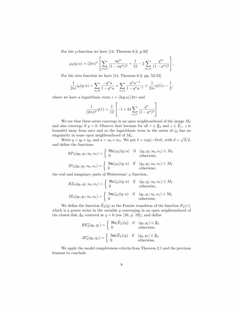
For the ℘-function we have [14, Theorem 6.2, p.50]

℘0(q;u) = (2πi)2

∑m∈Z

uqm

(1− uqm)2+

1

12− 2

∑m≥1

qm

(1− qm)2

,For the zeta function we have [14, Theorem 6.3, pp. 52-53]

1

2πiζ0(q;u) =

∑n≥0

−qnu1− qnu

+∑n≥1

qnu−1

1− qnu−1+

1

2πiη(1)z − 1

2,

where we have a logarithmic term z = (log u)/2πi and

1

(2πi)2η(1) =

1

12

−1 + 24∑n≥1

qn

(1− qn)2

We see that these series converge in an open neighbourhood of the image Mδ

and also converge if q = 0. Observe that because for all τ ∈ Fd and z ∈ Eτ , z isbounded away from zero and so the logarithmic term in the series of ζ0 has nosingularity in some open neighbourhood of Mδ.

Write q = q0 + iq1 and u = u0 + iu1. We put δ = exp(−2πd), with d =√

3/2,and define the functions

RP0(q0, q1;u0, u1) =

{Re(℘0)(q;u) if (q0, q1;u0, u1) ∈Mδ

0 otherwise,

IP0(q0, q1;u0, u1) =

{Im(℘0)(q;u) if (q0, q1;u0, u1) ∈Mδ

0 otherwise,

the real and imaginary parts of Weierstrass’ ℘ function,

RZ 0(q0, q1;u0, u1) =

{Re(ζ0)(q;u) if (q0, q1;u0, u1) ∈Mδ

0 otherwise,

IZ 0(q0, q1;u0, u1) =

{Im(ζ0)(q;u) if (q0, q1;u0, u1) ∈Mδ

0 otherwise,

We define the function E2(q) as the Fourier transform of the function E2(τ),which is a power series in the variable q converging in an open neighbourhood ofthe closed disk ∆δ centered at q = 0 (see [16, p. 19]), and define

RE∗2(q0, q1) =

{Re(E2)(q) if (q0, q1) ∈ Fd0 otherwise,

IE∗2(q0, q1) =

{Im(E2)(q) if (q0, q1) ∈ Fd0 otherwise,

We apply the model completeness criteria from Theorem 2.1 and the previouslemmas to conclude

8

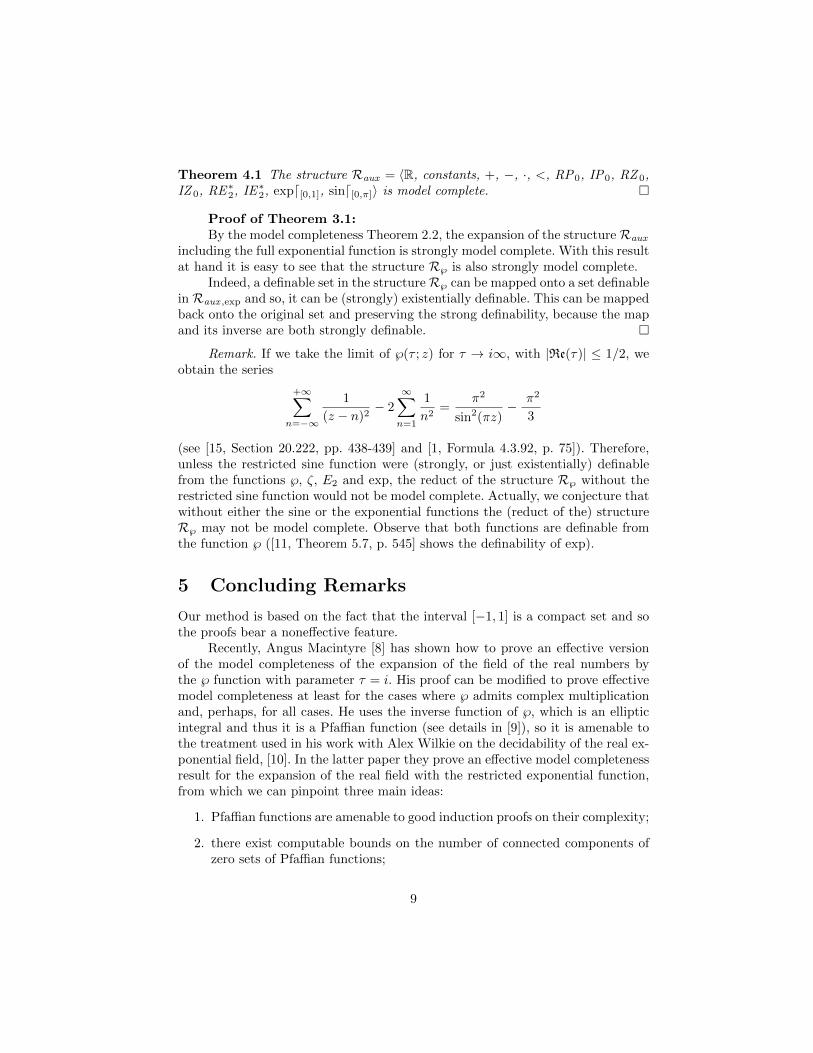
Theorem 4.1 The structure Raux = 〈R, constants, +, −, ·, <, RP0, IP0, RZ 0,IZ 0, RE∗2, IE∗2, expd[0,1], sind[0,π]〉 is model complete. �

Proof of Theorem 3.1:By the model completeness Theorem 2.2, the expansion of the structure Raux

including the full exponential function is strongly model complete. With this resultat hand it is easy to see that the structure R℘ is also strongly model complete.

Indeed, a definable set in the structureR℘ can be mapped onto a set definablein Raux ,exp and so, it can be (strongly) existentially definable. This can be mappedback onto the original set and preserving the strong definability, because the mapand its inverse are both strongly definable. �

Remark. If we take the limit of ℘(τ ; z) for τ → i∞, with |Re(τ)| ≤ 1/2, weobtain the series

+∞∑n=−∞

1

(z − n)2− 2

∞∑n=1

1

n2=

π2

sin2(πz)− π2

3

(see [15, Section 20.222, pp. 438-439] and [1, Formula 4.3.92, p. 75]). Therefore,unless the restricted sine function were (strongly, or just existentially) definablefrom the functions ℘, ζ, E2 and exp, the reduct of the structure R℘ without therestricted sine function would not be model complete. Actually, we conjecture thatwithout either the sine or the exponential functions the (reduct of the) structureR℘ may not be model complete. Observe that both functions are definable fromthe function ℘ ([11, Theorem 5.7, p. 545] shows the definability of exp).

5 Concluding Remarks

Our method is based on the fact that the interval [−1, 1] is a compact set and sothe proofs bear a noneffective feature.

Recently, Angus Macintyre [8] has shown how to prove an effective versionof the model completeness of the expansion of the field of the real numbers bythe ℘ function with parameter τ = i. His proof can be modified to prove effectivemodel completeness at least for the cases where ℘ admits complex multiplicationand, perhaps, for all cases. He uses the inverse function of ℘, which is an ellipticintegral and thus it is a Pfaffian function (see details in [9]), so it is amenable tothe treatment used in his work with Alex Wilkie on the decidability of the real ex-ponential field, [10]. In the latter paper they prove an effective model completenessresult for the expansion of the real field with the restricted exponential function,from which we can pinpoint three main ideas:

1. Pfaffian functions are amenable to good induction proofs on their complexity;

2. there exist computable bounds on the number of connected components ofzero sets of Pfaffian functions;

9

3. the structure is polynomially bounded and they showed that there is a com-putable estimate on the behaviour at infinity of the one-variable definablefunctions.

Their methods do not seem to apply to our case, because the derivative of ℘with respect to the parameter τ involves the modular forms E4 and E6 which arenot Pfaffian functions (but are noetherian functions) and satisfy nonlinear differen-tial equations involving E2, E4 and E6 in a (to our knowledge) nontriangularisableway.

Of the three items stated above, only the third one (behaviour at infinity)seems to be more easily achievable. There is some work towards the first and seconditem (computable bounds on the number of connected components) surveyed in[7].

AcknowledgementsThe author obtained good insights for this work from conversations with

his coleagues Oswaldo Rio Branco de Oliveira, who works on finding elementaryproofs of theorems in complex analysis, useful for model theoretic applications,and Paulo Agozzini Martin who shows us the beauty of arithmetic and analyticnumber theory.

References

[1] Milton Abramowitz, Irene A. Stegun (editors). Handbook of MathematicalFunctions with Formulas, Graphs, and Mathematical Tables. Ninth printingof 1965 edition, 1972. Dover Books on Mathematics, Dover Publications, Inc.,New York. MR1225604 (94b:00012)

[2] Ricardo Bianconi. Model completeness results for elliptic and abelian func-tions. Ann. Pure Appl. Logic 54 (2) (1991), 121-136. MR1134193 (92i:03040)

[3] Ricardo Bianconi. Model Complete Expansions of the Real Field by ModularFunctions and Forms. Submitted. 2014. (http://arxiv.org/abs/1406.7158)

[4] Jan Denef, Lou van den Dries. p-adic and real subanalytic sets. Ann. of Math.(2) 128 (1) (1988), 79-138. MR0951508 (89k:03034)

[5] Lou van den Dries. On the elementary theory of restricted elementary func-tions. J. Symbolic Logic 53 (3) (1988), 796-808. MR0960999 (89i:03074).

[6] Lou van den Dries, Angus Macintyre, David Marker. The elementary theoryof restricted analytic fields with exponentiation. Ann. of Math. (2) 140 (1)(1994), 183-205. MR1289495 (95k:12015)

[7] A. Gabrielov, N. Vorobjov. Complexity of computations with Pfaffian andNoetherian functions, in Normal Forms, Bifurcations and Finiteness Problemsin Differential Equations, 211-250, Kluwer, 2004. MR2083248 (2006b:14104)

10

[8] Angus Macintyre. The Elementary theory of elliptic functions I: the formal-ism and a special case. O-minimal Structures, Lisbon 2003. Proceedings of aSummer School by the European Research and Training Network, Mario J.Edmundo, Daniel Richardson, Alex Wilkie (eds.), RAAG. Available in (ac-cessed in March, 2014)

http://www.maths.manchester.ac.uk/raag/preprints/0159.pdf

[9] Angus Macintyre. Some observations about the real and imaginary parts ofcomplex Pfaffian functions. Model theory with applications to algebra andanalysis. Vol. 1, 215-223, London Math. Soc. Lecture Note Ser., 349, Cam-bridge Univ. Press, Cambridge, 2008. MR2441381 (2009h:03044)

[10] Angus Macintyre, A. J. Wilkie. On the decidability of the real exponentialfield. Kreiseliana, 441-467, A K Peters, Wellesley, MA, 1996. MR1435773

[11] Ya’acov Peterzil, Sergei Starchenko. Uniform definability of the Weierstrass ℘functions and generalized tori of dimension one. Selecta Math. (N.S.) 10 (4)(2004), 525-550. MR2134454 (2006d:03063)

[12] Johnathan Pila. O-minimality and the Andre-Oort conjecture for Cn. Annalsof Math. 173 (2011), 1779-1840. MR2800724 (2012j:11129)

[13] Johnathan Pila, Alex Wilkie. The rational points of a definable set. DukeMath. J. 133 (2006) 591-616. MR 2228464

[14] Joseph H. Silverman. Advanced topics in the arithmetic of elliptic curves.Graduate Texts in Mathematics, 151. Springer-Verlag, New York, 1994.xiv+525 pp. MR1312368 (96b:11074)

[15] E. T. Whittaker, G. N. Watson. A Course on Modern Analysis. An intro-duction to the general theory of infinite processes and of analytic functions;with an account of the principal transcendental functions. Reprint of thefourth (1927) edition. Cambridge Mathematical Library. Cambridge Univer-sity Press, Cambridge, 1996. vi+608 pp. MR1424469 (97k:01072)

[16] Don Zagier. Elliptic Modular Forms and Their Applications. The 1-2-3 ofModular Forms, Lectures at a Summer School in Nordfjordeid, Norway,Kristian Ranestad (ed), 2008 Springer-Verlag, Berlin, 1-103. MR2409678(2010b:11047)

11