a SpringerOpen Journal

Khan et al. SpringerPlus 2014, 3:724http://www.springerplus.com/content/3/1/724

RESEARCH Open Access

Exact solutions for (1 + 1)-dimensional nonlineardispersive modified Benjamin-Bona-Mahonyequation and coupled Klein-Gordon equationsKamruzzaman Khan1*, M Ali Akbar2 and S M Rayhanul Islam1

Abstract

In this work, recently developed modified simple equation (MSE) method is applied to find exact traveling wavesolutions of nonlinear evolution equations (NLEEs). To do so, we consider the (1 + 1)-dimensional nonlinear dispersivemodified Benjamin-Bona-Mahony (DMBBM) equation and coupled Klein-Gordon (cKG) equations. Two classes of explicitexact solutions–hyperbolic and trigonometric solutions of the associated equations are characterized with some freeparameters. Then these exact solutions correspond to solitary waves for particular values of the parameters.

Keywords: MSE method; NLEEs; DMBBM equation; cKG equation; Solitary wave; Exact solutions

PACS numbers: 02.30.Jr; 02.70.Wz; 05.45.Yv; 94.05.Fg

IntroductionThe study of NLEEs, i.e., partial differential equationswith time derivatives has a rich and long history, whichhas continued to attract attention in the last few decays.There are many examples throughout the world whereNLEEs play an important role in controlling the naturalsystems. Because the majority of the phenomena in realworld can be described by using NLEEs. NLEEs are fre-quently used to explain many problems of meteorology,population dynamics, fluid mechanics, plasma physics,optical fibers, biology, solid state physics, chemical kine-matics, geochemistry, nanotechnology etc. By the aid ofexact solutions, when they exist, the phenomena mod-eled by these NLEEs can be better understood. There-fore, the study of the traveling wave solutions for NLEEsplays an important role in the study of nonlinear phys-ical phenomena.In recent years, the exact solutions of NLEEs have

been investigated by many authors who are interested innonlinear physical phenomena. Many powerful methodshave been presented by diverse group of mathematiciansand physicists such as the Hirota’s bilinear transform-ation method (Hirota 1973) (Hirota and Satsuma 1981),

* Correspondence: k.khanru@gmail.com1Department of Mathematics, Pabna University of Science & Technology,Pabna 6600, BangladeshFull list of author information is available at the end of the article

© 2014 Khan et al.; licensee Springer. This is anAttribution License (http://creativecommons.orin any medium, provided the original work is p

the tanh-function method (Malfliet 1992; Nassar et al.2011), the F-expansion method (Zhou et al. 2003), the(G′/G)-expansion method (Wang et al. 2008; Zayed2010; Zayed and Al-Joudi 2010, Zayed and Gepreel2009; Akbar et al. 2012a, 2012b, 2012c, 2012d; Akbarand Ali 2011a; Shehata 2010; Zayed and Al-Joudi 2010;Naher et al. 2012a, 2013; Naher and Abdullah 2012,2013), the enhanced (G′/G)-expansion method (Khanet al. 2014, Khan and Akbar, 2014; Islam et al. 2014), theExp-function method (He and Wu 2006; Bekir and Boz2008; Akbar and Ali 2011b; Naher et al. 2011, 2012b;Yusufoglu 2008), the homogeneous balance method(Wang 1995; Zayed et al, 2004), the Adomian decompos-ition method (Adomian 1994), the homotopy perturbationmethod (Mohiud-Din 2007), the extended tanh-method(Abdou 2007; Fan 2000), the auxiliary equation method(Sirendaoreji 2004), the Jacobi elliptic function method(Ali 2011), Modified Exp-function method (He et al.2012), the Modified simple equation method (Jawad et al.2010; Zayed 2011; Zayed and Ibrahim 2012) and so on.The purpose of this paper is to apply the MSE method

to construct the exact solutions for nonlinear evolutionequations in mathematical physics via the DMBBMequation and cKG equation. The DMBBM equation andcKG equation are NLEEs representing the balance ofdispersion and weak nonlinearity in physical systemsthat generate solitary waves.

Open Access article distributed under the terms of the Creative Commonsg/licenses/by/4.0), which permits unrestricted use, distribution, and reproductionroperly credited.

Khan et al. SpringerPlus 2014, 3:724 Page 2 of 8http://www.springerplus.com/content/3/1/724

The article is prepared as follows: The MSE method,Applications, Graphical representation of some obtainedsolutions, Comparisons, and conclusions.

The MSE methodConsider a general nonlinear evolution in the form

ℜ u; ut ;ux; uy; uz; uxx; utt ;uxz; :::::� � ¼ 0 ð2:1Þ

where ℜ is a polynomial of u(x, y, z, t) and its partial de-rivatives in which the highest order derivatives and non-linear terms are involved. In the following, we give themain steps of this method (Jawad et al., 2010; Zayed,2011, Zayed and Ibrahim, 2012):Step 1. Using the traveling wave transformation

u x; y; z; tð Þ ¼ u ξð Þ; ξ ¼ xþ yþ z � ω t; ð2:2ÞEq. (2.1) transform to the following ODE:

℘ u;u′;u″;⋯ð Þ ¼ 0 ð2:3Þwhere ℘ is a polynomial in u(ξ) and its derivatives, while

u′ ξð Þ ¼ ddξ, u″ ξð Þ ¼ d2

dξ2;and so on.

Step 2. We suppose that Eq.(2.3) has the formal solution

u ξð Þ ¼ β0 þXNk¼1

β kΦ′ ξð ÞΦ ξð Þ� �k

ð2:4Þ

where βk are arbitrary constants to be determined, suchthat βN ≠ 0, and Φ(ξ) is an unknown function to be de-termined later.Step 3. We determine the positive integer N in Eq. (2.4)

by considering the homogeneous balance between thehighest order derivatives and the nonlinear terms inEq. (2.3).Step 4. We substitute (2.4) into (2.3), we calculate all

the necessary derivatives u′ , u″ ,⋯ and then we accountthe function Φ(ξ). As a result of this substitution, we geta polynomial of Φ′(ξ)/Φ(ξ) and its derivatives. In thispolynomial, we equate with zero all the coefficients ofΦ− i(ξ), where i = 0, 1, 2,⋯. This operation yields a sys-tem of equations which can be solved to find βk andΦ(ξ). Consequently, we can get the exact solutions ofEq. (2.1).

ApplicationsThe (1 + 1)-dimensional nonlinear dispersive modifiedBenjamin-BonaMahony equation: In this section, we will apply themodified simple equation method to find the exact solu-tions and then the solitary wave solutions of (1 + 1)-dimensional nonlinear DMBBM equation,

ut þ ux−αu2ux þ uxxx ¼ 0 ð3:1Þ

where α is a nonzero constant. This equation was firstderived to describe an approximation for surface longwaves in nonlinear dispersive media. It can also char-acterize the hydro magnetic waves in cold plasma,acoustic waves in inharmonic crystals and acoustic grav-ity waves in compressible fluids (Yusufoglu 2008; Zayedand Al-Joudi 2010).The traveling wave transformation is

u ¼ u x; tð Þ; ξ ¼ x−ω t; u ¼ u ξð Þ; u x; tð Þ ¼ u ξð Þð3:2Þ

Using traveling wave Eq. (3.2), Eq. (3.1) transformsinto the following ODE

1−ωð Þu′−αu2u′þ u‴ ¼ 0 ð3:3ÞIntegrating with respect to ξ choosing constant of inte-

gration as zero, we obtain the following ODE

3 1−ωð Þu−αu3 þ 3u″ ¼ 0 ð3:4ÞNow balancing the highest order derivative u″ and

non-linear term u3, we get3N =N + 2, which gives N = 1

Now for N = 1, u ξð Þ ¼ β0 þXNk¼1

β kΦ′ ξð ÞΦ ξð Þh ik

becomes

u ξð Þ ¼ β0 þ β1Φ′

Φ

� �ð3:5Þ

where β0 and β1 are constants to be determined suchthat β1 ≠ 0, while ψ(ξ) is an unknown function to be de-termined. It is easy to see that

u″ ¼ β1Φ‴

Φ−3β1

Φ″Φ′

Φ2 þ 2β1Φ′

Φ

� �3

ð3:6Þ

u3 ¼ β13 Φ′

Φ

� �3

þ 3β12β0

Φ′

Φ

� �2

þ 3β1β02 Φ′

Φ

� �þ β0

3

ð3:7ÞNow substituting the values of u″, u, u3 in equation (3.3)

and then equating the coefficients of Φ0,Φ− 1,Φ− 2,Φ− 3 tozero, we respectively obtain

αβ03−3 1−ωð Þβ0 ¼ 0 ð3:8Þ

Φ‴− ωþ αβ02−1

� �Φ′ ¼ 0 ð3:9Þ

3Φ″þ αβ0β1Φ′ ¼ 0 ð3:10Þ

6β1−αβ13� �Φ′3 ¼ 0 ð3:11Þ

Khan et al. SpringerPlus 2014, 3:724 Page 3 of 8http://www.springerplus.com/content/3/1/724

Solving Eq. (3.8), we get

β0 ¼ 0;�ffiffiffiffiffiffiffiffiffiffiffiffiffiffiffi3 1−ωð Þ

α

r

Solving Eq. (3.11), we get

β1 ¼ �ffiffi6α

qand β1 ≠ 0

Case I: when β0 = 0 solving Eqs. (3.9), and (3.10) weget trivial solution. So this case is rejected.

Case II: when β0 ¼ �ffiffiffiffiffiffiffiffiffiffiffi3 1−ωð Þ

α

q, Eqs. (3.9) and (3.10) yields

Φ‴þ lΦ″ ¼ 0 ð3:12Þ

where l ¼ ffiffiffiffiffiffiffiffiffiffiffiffiffiffiffiffiffiffiffi2 1−ωð Þð Þp

.Integrating, Eq. (3.12) with respect to ξ, we obtain

Φ″ ¼ c1 exp −l ξð Þ ð3:13Þ

From Eqs. (3.13) and (3.10), we obtain

Φ′ ¼ −c1 exp −l ξð Þffiffiffiffiffiffiffiffiffiffiffiffiffiffiffiffiffiffiffi2 1−ωð Þð Þp ð3:14Þ

Therefore, upon integration, we obtain

Φ ¼ c2−c1 exp −l ξð Þ2 1−ωð Þ ð3:15Þ

where c1 and c2 are arbitrary constants.Substituting the values of Φ and Φ′ into Eq. (3.5), we

obtain the following exact solution,

u ξð Þ ¼ β0 þ β1−2 1−ωð Þc1 exp −l ξð Þffiffiffiffiffiffiffiffiffiffiffiffiffiffiffi

2 1−ωð Þp2 1−ωð Þc2 þ c1 exp −l ξð Þð Þ

ð3:16ÞPutting the values of β0, β1, l and simplifying, we obtain

u x ; tð Þ ¼ �ffiffiffiffiffiffiffiffiffiffiffiffiffiffiffi3 1−ωð Þ

α

r

� 1−

2 c1

cosh

ffiffiffiffiffiffiffiffiffiffiffiffiffiffiffiffiffiffiffiffi1−ωð Þ2

� �sx−ω tð Þ

!

− sinh

ffiffiffiffiffiffiffiffiffiffiffiffiffiffiffiffiffiffiffiffi1−ωð Þ2

� �sx−ω tð Þ

!0BBBB@

1CCCCA

2 1−ωð Þc2−c1ð Þ coshffiffiffiffiffiffiffiffiffiffiffiffiffiffiffiffiffiffiffiffi

1−ωð Þ2

� �sx−ω tð Þ

!

þ 2 1−ωð Þc2 þ c1ð Þ sinhffiffiffiffiffiffiffiffiffiffiffiffiffiffiffiffiffiffiffiffi

1−ωð Þ2

� �sx−ω tð Þ

!

0BBBBBBBBBBBBBBBB@

1CCCCCCCCCCCCCCCCA

ð3:17Þ

Since c1 and c2 are arbitrarily constants, consequently, if

we set c1 = − 2 c2(1 −ω) and 1−ωð Þ2 > 0 , Eq. (3.17) reduces

to the following traveling wave solution:

u1;2 x; tð Þ ¼ �ffiffiffiffiffiffiffiffiffiffiffiffiffiffiffiffiffiffiffiffiffiffi3 1−ωð Þ

α

� �stanh

ffiffiffiffiffiffiffiffiffiffiffiffiffiffiffiffiffiffiffiffi1−ωð Þ2

� �sx−ω tð Þ

!

ð3:18Þ

Again setting c1 = 2 c2(1 −ω) and if 1−ωð Þ2 > 0, Eq. (3.17)

reduces to the following singular traveling wave solutions:

u3;4 x; tð Þ ¼ �ffiffiffiffiffiffiffiffiffiffiffiffiffiffiffiffiffiffiffiffiffiffi3 1−ωð Þ

α

� �scoth

ffiffiffiffiffiffiffiffiffiffiffiffiffiffiffiffiffiffiffiffi1−ωð Þ2

� �sx−ω tð Þ

!

ð3:19Þ

If 1−ωð Þ2 < 0, Eqs. (3.18) and (3.19) yields the following

periodic solutions:

u5;6 x; tð Þ ¼ �ffiffiffiffiffiffiffiffiffiffiffiffiffiffiffiffiffiffiffiffiffiffi3 ω−1ð Þ

α

� �stan

ffiffiffiffiffiffiffiffiffiffiffiffiffiffiffiffiffiffiffiffiω−1ð Þ2

� �sx−ω tð Þ

!;

ð3:20Þand

u7;8 x; tð Þ ¼ �ffiffiffiffiffiffiffiffiffiffiffiffiffiffiffiffiffiffiffiffiffiffi3 ω−1ð Þ

α

� �scot

ffiffiffiffiffiffiffiffiffiffiffiffiffiffiffiffiffiffiffiffiω−1ð Þ2

� �sx−ω tð Þ

!:

ð3:21ÞRemark 1: From solutions (3.18)-(3.21) we conclude

that ω ≠ 1.

The coupled Klein-Gordon equationNow we will bring to bear the MSE method to find exactsolutions and then the solitary wave solutions to thecKG Equation in the form,

ux x−ut t−uþ 2u3 þ 2uv ¼ 0;vx−vt−4uut ¼ 0

ð3:22Þ

where

u ξð Þ ¼ u x; tð Þ; v ξð Þ ¼ v x; tð Þ; ξ ¼ x−ω t: ð3:23ÞThe traveling wave Eq. (3.23) reduces Eqs. (3.22) into

the following ODEs

1−ω2� �

u″−uþ 2u3 þ 2uv ¼ 0 ð3:24Þ1þ ωð Þv′þ 4ωuu′ ¼ 0 ð3:25Þ

By integrating Eq. (3.25) with respect to ξ, and neglect-ing the constant of integration we obtain

v ¼ −2ω

1þ ωu2: ð3:26Þ

Khan et al. SpringerPlus 2014, 3:724 Page 4 of 8http://www.springerplus.com/content/3/1/724

Substituting Eq. (3.26) into Eq. (3.24) we get,

1−ω2� �

u″−uþ 2 1−ωð Þ1þ ω

u3 ¼ 0: ð3:27Þ

Balancing the highest order derivative u″ and nonlin-ear term u3 from Eq. (3.27), we obtain N = 1Now for N = 1, Eq. (2.4) becomes

u ξð Þ ¼ β0 þ β1Φ′

Φ

� �ð3:28Þ

where β0 and β1 are constants to be determined suchthat β1 ≠ 0, while Φ(ξ) is an unknown function to be de-termined. It is easy to see that

u″ ¼ β1Φ‴

Φ−3β1

Φ″Φ′

Φ2 þ 2β1Φ′

Φ

� �3

ð3:29Þ

u3 ¼ β13 Φ′

Φ

� �3

þ 3β12β0

Φ′

Φ

� �2

þ 3β1β02 Φ′

Φ

� �þ β0

3:

ð3:30ÞNow substituting the values of u″, u, u3 in Eq. (3.27)

and then equating the coefficients of Φ0,Φ− 1,Φ− 2,Φ− 3

to zero, we respectively obtain

β03 2

1þ ω−

2ω1þ ω

� �−β0 ¼ 0 ð3:31Þ

1−ω2� �

Φ″−2β0 β1 1−ωð Þ

1þ ω

� �Φ′ ¼ 0 ð3:32Þ

1−ω2� �

Φ‴þ 6β20 1−ωð Þ1þ ω

−1� �

Φ′ ¼ 0 ð3:33Þ

−2ω2β1 þ 2β1 þ2β1

3

1þ ω−2ωβ1

3

1þ ω¼ 0: ð3:34Þ

Solving Eq. (3.31), we get

β0 ¼ 0;�ffiffiffiffiffiffiffiffiffiffiffiffiffiffiffiffiffiffiffiffiffiffi

1þ ω

2 1−ωð Þ� �s

Solving Eq. (3.34), we get

β1 ¼ �I 1þ ωð Þ andβ1≠0; I ¼ffiffiffiffiffiffi−1

p

Case-I: When β0 = 0, Eq. (3.32) and (3.33) yields a trivialsolution. So this case is rejected.

Case-II: When β0 ¼ �ffiffiffiffiffiffiffiffiffiffiffi1þωð Þ

2 1−ωð Þq

, Eqs. (3.32) and (3.33)

yields,

Φ‴−I

ffiffiffiffiffiffiffiffiffiffiffiffiffiffiffiffiffiffi1−ω2

2

� �sΦ″ ¼ 0 ð3:35Þ

Integrating, Eq. (3.35) with respect to ξ, we obtain

Φ″ ¼ c1 exp I

ffiffiffiffiffiffiffiffiffiffiffiffiffiffiffiffiffiffi2

1−ω2

� �sξ

!: ð3:36Þ

From Eqs. (3.36) and (3.32), we obtain

Φ′ ¼ −I

ffiffiffiffiffiffiffiffiffiffiffiffiffiffiffiffiffiffi1−ω2

2

� �sc1 exp I

ffiffiffiffiffiffiffiffiffiffiffiffiffiffiffiffiffiffi2

1−ω2

� �sξ

!: ð3:37Þ

Therefore, integration Eq. (3.37), we obtain

Φ ¼ 12

2c2− 1−ω2� �

c1 exp I

ffiffiffiffiffiffiffiffiffiffiffiffiffiffiffiffiffiffi2

1−ω2

� �sξ

! !;

ð3:38Þwhere c1 and c2 are constants of integration.Substituting the values of Φ and Φ′ into Eq. (3.28), we

obtain the following exact solution,

u ξð Þ ¼ β0−β1Iffiffiffiffiffiffiffiffiffiffiffiffiffiffiffiffiffi2 1−ω2ð Þp

c1 exp Iffiffiffiffiffiffiffiffiffiffiffiffi

21−ω2

� �qξ

2c2− 1−ω2ð Þc1 exp I

ffiffiffiffiffiffiffiffiffiffiffiffi2

1−ω2

� �qξ

:ð3:39Þ

Putting the values of β0, β1 into Eq. (3.39) and thensimplifying, we obtain

u x; tð Þ ¼ffiffiffiffiffiffiffiffiffiffiffiffiffiffiffiffiffiffiffiffiffiffi

1þ ω

2 1−ωð Þ� �s

� 1þ

2 1−ω2ð Þc1cosh

Iffiffiffiffiffiffiffiffiffiffiffiffiffiffiffiffiffi2 1−ω2ð Þp x−ω tð Þ

!

þ sinhIffiffiffiffiffiffiffiffiffiffiffiffiffiffiffiffiffi

2 1−ω2ð Þp x−ω tð Þ !

0BBBB@

1CCCCA

2 c2− 1−ω2ð Þ c1ð Þ cosh Iffiffiffiffiffiffiffiffiffiffiffiffiffiffiffiffiffi2 1−ω2ð Þp x−ω tð Þ

!

− 2c2− 1−ω2ð Þc1ð Þ sinh Iffiffiffiffiffiffiffiffiffiffiffiffiffiffiffiffiffi2 1−ω2ð Þp x−ω tð Þ

!

0BBBBBBBBBBBBBBB@

1CCCCCCCCCCCCCCCA

:

ð3:40Þ

We can freely choose the constants c1 and c2. There-

fore, if we set c2 ¼ 1−ω2ð Þ c12 , Eq. (3.40) reduces to:

u1;2 x; tð Þ ¼ �ffiffiffiffiffiffiffiffiffiffiffiffiffiffiffiffiffiffiffiffiffiffi

1þ ω

2 1−ωð Þ� �s

cothI x−ω tð Þffiffiffiffiffiffiffiffiffiffiffiffiffiffiffiffiffi2 1−ω2ð Þp

!:

ð3:41Þ

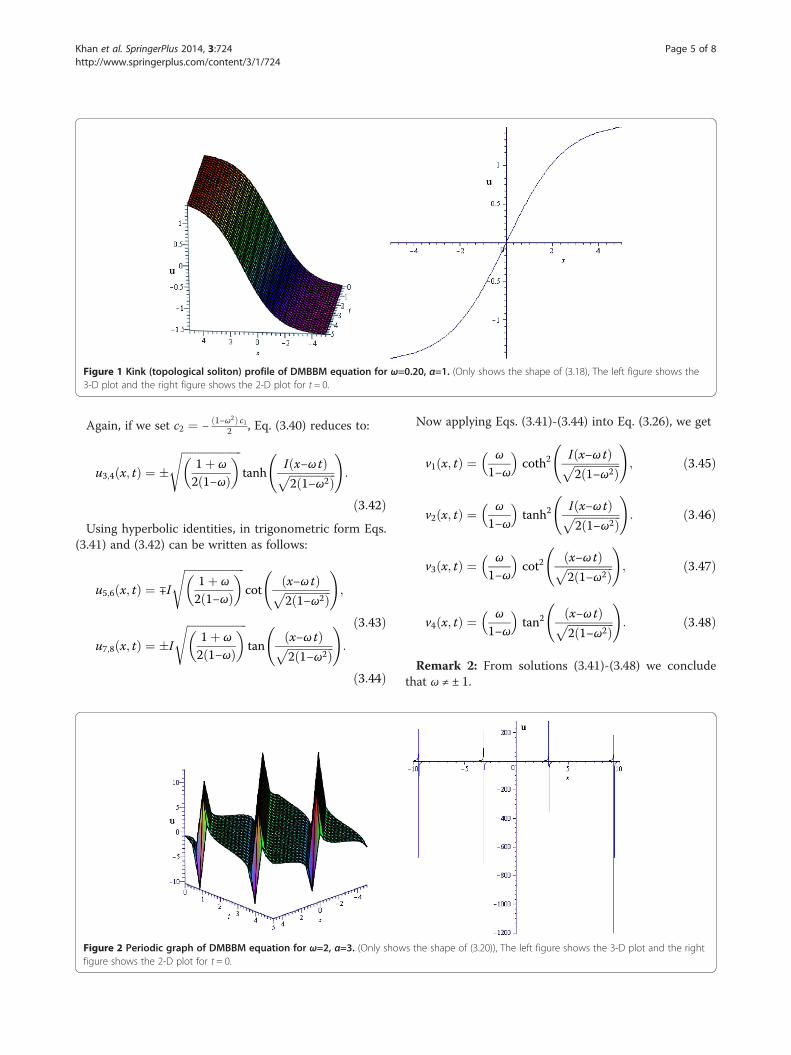
Figure 1 Kink (topological soliton) profile of DMBBM equation for ω=0.20, α=1. (Only shows the shape of (3.18), The left figure shows the3-D plot and the right figure shows the 2-D plot for t = 0.

Khan et al. SpringerPlus 2014, 3:724 Page 5 of 8http://www.springerplus.com/content/3/1/724

Again, if we set c2 ¼ − 1−ω2ð Þ c12 , Eq. (3.40) reduces to:

u3;4 x; tð Þ ¼ �ffiffiffiffiffiffiffiffiffiffiffiffiffiffiffiffiffiffiffiffiffiffi

1þ ω

2 1−ωð Þ� �s

tanhI x−ω tð Þffiffiffiffiffiffiffiffiffiffiffiffiffiffiffiffiffi2 1−ω2ð Þp

!:

ð3:42ÞUsing hyperbolic identities, in trigonometric form Eqs.

(3.41) and (3.42) can be written as follows:

u5;6 x; tð Þ ¼ ∓I

ffiffiffiffiffiffiffiffiffiffiffiffiffiffiffiffiffiffiffiffiffiffi1þ ω

2 1−ωð Þ� �s

cotx−ω tð Þffiffiffiffiffiffiffiffiffiffiffiffiffiffiffiffiffi2 1−ω2ð Þp

!;

ð3:43Þu7;8 x; tð Þ ¼ �I

ffiffiffiffiffiffiffiffiffiffiffiffiffiffiffiffiffiffiffiffiffiffi1þ ω

2 1−ωð Þ� �s

tanx−ω tð Þffiffiffiffiffiffiffiffiffiffiffiffiffiffiffiffiffi2 1−ω2ð Þp

!:

ð3:44Þ

Figure 2 Periodic graph of DMBBM equation for ω=2, α=3. (Only showfigure shows the 2-D plot for t = 0.

Now applying Eqs. (3.41)-(3.44) into Eq. (3.26), we get

v1 x; tð Þ ¼ ω

1−ω

coth2

I x−ω tð Þffiffiffiffiffiffiffiffiffiffiffiffiffiffiffiffiffi2 1−ω2ð Þp

!; ð3:45Þ

v2 x; tð Þ ¼ ω

1−ω

tanh2

I x−ω tð Þffiffiffiffiffiffiffiffiffiffiffiffiffiffiffiffiffi2 1−ω2ð Þp

!: ð3:46Þ

v3 x; tð Þ ¼ ω

1−ω

cot2

x−ω tð Þffiffiffiffiffiffiffiffiffiffiffiffiffiffiffiffiffi2 1−ω2ð Þp

!; ð3:47Þ

v4 x; tð Þ ¼ ω

1−ω

tan2

x−ω tð Þffiffiffiffiffiffiffiffiffiffiffiffiffiffiffiffiffi2 1−ω2ð Þp

!: ð3:48Þ

Remark 2: From solutions (3.41)-(3.48) we concludethat ω ≠ ± 1.

s the shape of (3.20)), The left figure shows the 3-D plot and the right

Figure 3 Bell (non- topological soliton) profile of cKG equation for ω=1.50. (Only shows the shape of solution (3.46)), The left figure showsthe 3-D plot and the right figure shows the 2-D plot for t = 0.

Khan et al. SpringerPlus 2014, 3:724 Page 6 of 8http://www.springerplus.com/content/3/1/724

Graphical representation of some obtainedsolutionsIn this section, we put forth to illustrate the three-dimensional and two-dimensional structure of the deter-mined solutions of the studied NLEEs, to visualize theinner mechanism of them.Figure 1 and Figure 2 represent the shape of solutions

(3.18) and (3.20) of DMBBM equation. On the otherhand, Figure 3 and Figure 4 show the profile of solutions(3.46) and (3.48) of cKG equation.

ComparisonsWith extended (G′/G)-expansion method:Zayed and Al-Joudi (2010) investigated exact solutions

of the traveling wave solutions of the DMBBM equationby using the extended (G′/G)-expansion method andobtained six solutions. On the contrary by using theMSE method in this article we obtained eight solutions.

Figure 4 Periodic profile of cKG equation for ω=0.75. (Only shows theshows the 2-D plot for t = 0.

However, Some of the solutions obtained by Zayed andAl-Joudi (2010) coincide with our solutions. If we set ω =1 + 2μ in our solutions (3.18) and (3.19), we conclude thatour results coincide to the solution (3.9) obtained byZayed and Al-Joudi (2010) for A ≠ 0,B = 0, μ < 0, σ = ± 1and A = 0,B ≠ 0, μ < 0, σ = ± 1 respectively. Similarly, solu-tions (3.20) and (3.21) obtained in this article correspondto the solution (3.12) obtained by Zayed and Al-Joudi(2010) for A ≠ 0,B = 0, μ > 0, σ = ± 1 and A = 0,B ≠ 0, μ > 0,σ = ± 1 respectively.Moreover, Zayed and Al-Joudi (2010) used the symbolic

computation software such as Maple or Mathematica tofacilitate the calculation of the algebraic equations oc-curred in the solution procedure. Without symbolic com-putation software even it is impossible to get the solutionsof the complicated algebraic equations. In addition, Zayedand Al-Joudi (2010) used the solutions of an auxiliaryequation G″(ξ) + μG(ξ) = 0 to find exact traveling wave

shape of (3.48)), The left figure shows the 3-D plot and the right figure

Khan et al. SpringerPlus 2014, 3:724 Page 7 of 8http://www.springerplus.com/content/3/1/724

solutions of NLEEs. On the other hand it is worth men-tioning that the exact solutions of the studied NLEEs havebeen achieved in this article without using any symboliccomputations software, since the computations are verysimple and easy. Similarly for any nonlinear evolutionequation it can be shown that the MSE method is mucheasier than other methods. Furthermore, auxiliary equa-tions are unnecessary to solve NLEEs by means of MSEmethods, i.e., there exists no predefined functions or equa-tions in MSE method.

ConclusionsThis study shows that the MSE method is quite efficientand practically well suited for use to find exact travelingwave solutions of the DMBBM equation and cKG equa-tion. We have obtained exact solutions of these equa-tions in terms of the hyperbolic and trigonometricfunctions. This study also shows that the procedure issimple, direct and constructive. The reliability of themethod and the reduction in the size of computationaldomain give this method a wider applicability. We con-clude that the studied method can be used for manyother NLEEs in mathematical physics and engineeringfields.

Competing interestsThe authors declare that they have no competing interests.

Authors’ contributionsThis work was carried out in collaboration among the authors. All authorshave a good contribution to design the study, and to perform the analysisof this research work. All authors read and approved the final manuscript.

Author details1Department of Mathematics, Pabna University of Science & Technology,Pabna 6600, Bangladesh. 2Department of Applied Mathematics, University ofRajshahi, Rajshahi 6205, Bangladesh.

Received: 27 August 2014 Accepted: 20 November 2014Published: 10 December 2014

ReferencesAbdou MA (2007) The extended tanh-method and its applications for solving

nonlinear physical models. App Math Comput 190:988–996Adomian G (1994) Solving frontier problems of physics: The decomposition

method. Kluwer Academic, Boston, M AAkbar MA, Ali NHM, Zayed EME (2012a) Abundant exact traveling wave solutions

of the generalized Bretherton equation via (G′/G)-expansion method.Commun Theor Phys 57:173–178

Akbar MA, Ali NHM, Zayed EME (2012b) A generalized and improved (G′/G)-expansion method for nonlinear evolution equations. Math Prob Engr2012:22, doi:10.1155/2012/459879

Akbar MA, Ali NHM, Mohyud-Din ST (2012c) The alternative (G′/G)- expansionmethod with generalized Riccati equation: Application to fifth order (1+1)-dimensional Caudrey-Dodd-Gibbon equation. Int J Phys Sci 7(5):743–752

Akbar MA, Ali NHM, Mohyud-Din ST (2012d) Some new exact traveling wavesolutions to the (3 + 1)-dimensional Kadomtsev-Petviashvili equation. WorldAppl Sci J 16(11):1551–1558

Akbar MA, Ali NHM (2011a) The alternative (G′/G)-expansion method and itsapplications to nonlinear partial differential equations. Int J Phys Sci6(35):7910–7920

Akbar MA, Ali NHM (2011b) Exp-function method for Duffing Equation and newsolutions of (2 + 1) dimensional dispersive long wave equations. Prog ApplMath 1(2):30–42

Ali AT (2011) New generalized Jacobi elliptic function rational expansion method.J Comput Appl Math 235:4117–4127

Bekir A, Boz A (2008) Exact solutions for nonlinear evolution equations usingExp- function method. Phys Lett 372:1619–1625

Fan EG (2000) Extended tanh-method and its applications to nonlinear equations.Phys Lett 277:212–218

He Y, Li S, Long Y (2012) Exact solutions of the Klein-Gordon equation bymodified Exp-function method. Int Math Forum 7(4):175–182

He JH, Wu XH (2006) Exp-function method for nonlinear wave equations. Chaos,Solitons and Fract 30:700–708

Hirota R (1973) Exact envelope soliton solutions of a nonlinear wave equation.J Math Phy 14:805–810

Hirota R, Satsuma J (1981) Soliton solutions of a coupled KDV equation. Phy LettA 85:404–408

Islam MH, Khan K, Akbar MA, Salam MA (2014) Exact Traveling Wave Solutions ofModified KdV–Zakharov–Kuznetsov Equation and Viscous Burgers Equation.SpringerPlus 3:105, doi:10.1186/2193-1801-3-105

Jawad AJM, Petkovic MD, Biswas A (2010) Modified simple equation method fornonlinear evolution equations. Appl Math Comput 217:869–877

Khan K, Akbar MA, Salam MA, Islam MH (2014) A note on enhanced (G′/G)-expansion method in nonlinear physics. Ain Shams Engineering Journal5:877–884, http://dx.doi.org/10.1016/j.asej.2013.12.013

Khan K, Akbar MA (2014) Study of analytical method to seek for exact solutionsof variant Boussinesq equations. SpringerPlus 3:324, doi:10.1186/2193-1801-3-324

Malfliet M (1992) Solitary wave solutions of nonlinear wave equations. Am J Phys60:650–654

Mohiud-Din ST (2007) Homotopy perturbation method for solving fourth-orderboundary value problems. Math Prob Engr 2007:1–15, Article ID 98602,doi:10.1155/2007/98602

Naher H, Abdullah AF, Akbar MA (2012a) New traveling wave solutions of thehigher dimensional nonlinear partial differential equation by theExp-function method. J Appl Math, Article ID 575387, 14 pages. doi:10.1155/2012/575387

Naher H, Abdullah AF, Akbar MA (2011) The Exp-function method for new exactsolutions of the nonlinear partial differential equations. Int J Phys Sci6(29):6706–6716

Naher H, Abdullah FA, Bekir A (2012b) Abundant traveling wave solutions of thecompound KdV-Burgers equation via the improved (G′/G)-expansionmethod. AIP Adv, 2, 042163. http://dx.doi.org/10.1063/1.4769751

Naher H, Abdullah FA, Akbar MA (2013) Generalized and improved (G′/G)-expansion method for (3 + 1)-dimensional modified KdV–Zakharov–Kuznetsev equation. PLoS One 8(5):e64618

Naher H, Abdullah FA (2012) Some new traveling wave solutions of the nonlinearreaction diffusion equation by using the improved (G′/G)-expansion method.Math Prob Engr 2012:17, http://dx.doi.org/10.1155/2012/871724

Naher H, Abdullah FA (2013) New approach of (G′/G)-expansion method andnew approach of generalized (G′/G)-expansion method for nonlinearevolution equation. AIP Adv 3(3):032116

Nassar HA, Abdel-Razek MA, Seddeek AK (2011) Expanding the tanh-functionmethod for solving nonlinear equations. Appl Math 2:1096–1104

Shehata AR (2010) The traveling wave solutions of the perturbed nonlinearSchrodinger equation and the cubic-quintic Ginzburg Landau equation usingthe modified (G′/G)-expansion method. Appl Math Comput 217:1–10

Sirendaoreji (2004) New exact travelling wave solutions for the Kawahara andmodified Kawahara equations. Chaos Solitons Fract 19:147–150

Wang M (1995) Solitary wave solutions for variant Boussinesq equations. PhysLett 199:169–172

Wang M, Li X, Zhang J (2008) The (G′/G)-expansion method and travelling wavesolutions of nonlinear evolution equations in mathematical physics. Phys Lett372:417–423

Yusufoglu E (2008) New solitary solutions for the MBBM equations usingExp-function method. Phys Lett 372:442–446

Zayed EME (2011) A note on the modified simple equation method applied toSharma- Tasso-Olver equation. Appl Math Comput 218:3962–3964

Zayed EME, Ibrahim SAH (2012) Exact solutions of nonlinear evolution equationsin Mathematical physics using the modified simple equation method.Chinese Phys Lett 29(6):060201

Zayed EME, Zedan HA, Gepreel KA (2004) On the solitary wave solutions fornonlinear Hirota-Sasuma coupled KDV equations. Chaos, Solitons and Fractals22:285–303

Khan et al. SpringerPlus 2014, 3:724 Page 8 of 8http://www.springerplus.com/content/3/1/724

Zayed EME, Al-Joudi S (2010) Applications of an extended (G′/G)-expansionmethod to find exact solutions of nonlinear PDEs in mathematical physics.Math Prob Engr, 19 pages, doi:10.1155/2010/768573

Zayed EME (2010) Traveling wave solutions for higher dimensional nonlinearevolution equations using the (G′/G)-expansion method. J Appl MathInformatics 28:383–395

Zayed EME, Gepreel KA (2009) The (G′/G)-expansion method for finding thetraveling wave solutions of nonlinear partial differential equations inmathematical physics. J Math Phys 50:013502–013514

Zhou YB, Wang ML, Wang YM (2003) Periodic wave solutions to coupled KdVequations with variable coefficients. Phys Lett 308:31–36

doi:10.1186/2193-1801-3-724Cite this article as: Khan et al.: Exact solutions for (1 + 1)-dimensionalnonlinear dispersive modified Benjamin-Bona-Mahony equation andcoupled Klein-Gordon equations. SpringerPlus 2014 3:724.

Submit your manuscript to a journal and benefi t from:

7 Convenient online submission

7 Rigorous peer review

7 Immediate publication on acceptance

7 Open access: articles freely available online

7 High visibility within the fi eld

7 Retaining the copyright to your article

Submit your next manuscript at 7 springeropen.com