Self-normalized central limit theorem for sums of weakly dependent random variables
30
Journal of Theoretical Probability, Vol. 7, No. 2, 1994 Self-Normalized Central Limit Theorem for Sums of Weakly Dependent Random Variables Magda Peligrad 1 and Qi-Man Shao 2 Received June 17, 1992; revised September 24, 1993 Let {X., n >t 1 } be a strictly stationary sequence of weakly dependent random variables satisfying EX. = #, EX2. < oo, Vat S./n --*a 2 > 0 and the central limit theorem. This paper presents two estimators of tr2. Their weak and strong consistence as well as their rate of convergence are obtained for a-mixing, p-mixing and associated sequences. KEY WORDS: Central limit theorem; weakly dependent random variables. 1. INTRODUCTION Let {X,,, n/> 1 } be a strictly stationary sequence of random variables with EX,, =/~. Under some dependence and moment conditions, various strong laws of large numbers are well-known, that is 1 i .r := - Xj---, # a.s. as n ~ oo (1.1) n j=l If EX~ < oo and Var S,,/n ~ a 2 for some positive a as n--* oo, the well- known central limit theorem gives the rate of convergence of the sample mean ~,, to #, i.e. n(X,,- I.t) , U~O, 1) (1.1) t Supported by a NSF grant and a Taft travel grant. Department of Mathematical Sciences, University of Cincinnati, Cincinnati, Ohio 45221-0025. 2 Supported by a Taft Post-doctoral Fellowship at the University of Cincinnati and by the Fok Yingtung Education Foundation of China. Hangzhou University, Hangzhou, Zhejiang, P.R. China and Department of Mathematics, National University of Singapore, Singapore 0511. 3O9 0894-9840/94/0400-0309507.00/0 1994PlenumPublishing Corporation
-
Upload
independent -
Category
Documents
-
view
2 -
download
0
Transcript of Self-normalized central limit theorem for sums of weakly dependent random variables

Journal of Theoretical Probability, Vol. 7, No. 2, 1994
Self-Normalized Central Limit Theorem for Sums of Weakly Dependent Random Variables
M a g d a Peligrad 1 and Qi-Man Shao 2
Received June 17, 1992; revised September 24, 1993
Let {X., n >t 1 } be a strictly stationary sequence of weakly dependent random variables satisfying EX. = #, EX2. < oo, Vat S./n --* a 2 > 0 and the central limit theorem. This paper presents two estimators of tr 2. Their weak and strong consistence as well as their rate of convergence are obtained for a-mixing, p-mixing and associated sequences.
KEY WORDS: Central limit theorem; weakly dependent random variables.
1. INTRODUCTION
Let {X,,, n/> 1 } be a strictly stationary sequence of random variables with EX,, =/~. Under some dependence and moment conditions, various strong laws of large numbers are well-known, that is
1 i .r : = - Xj---, # a.s. as n ~ oo (1.1) n j = l
If EX~ < oo a n d Var S,,/n ~ a 2 for s o m e pos i t ive a as n--* oo, the well-
k n o w n central limit theorem gives the rate of convergence of the sample m e a n ~,, to #, i.e.
n ( X , , - I.t) , U~O, 1) (1.1)
t Supported by a NSF grant and a Taft travel grant. Department of Mathematical Sciences, University of Cincinnati, Cincinnati, Ohio 45221-0025.
2 Supported by a Taft Post-doctoral Fellowship at the University of Cincinnati and by the Fok Yingtung Education Foundation of China. Hangzhou University, Hangzhou, Zhejiang, P.R. China and Department of Mathematics, National University of Singapore, Singapore 0511.
3O9
0894-9840/94/0400-0309507.00/0 �9 1994 Plenum Publishing Corporation

310 Peligrad and Shao
where N(0, 1) is a standard normal random variable and ~ denotes con- vergences in distribution. However, in general a is not known in practice and should be estimated from the data in order to make the central limit theorem applicable.
The aim of this paper is to introduce two estimators of a and to investigate their weak and strong consistence and the rate of their convergence to or. We first list some definitions of dependence structures for easy reference.
Let {X. , n >1 1 } be a sequence of random variables and F~ denote the a-field generated by the random variables Xa, Xa+l ..... Xb. The sequence {X., n/> 1 } is called strongly mixing or a-mixing if
a (n )= sup IP (AB) - -P (A)P(B) I -+O as n ~ o o k>.l ,A~f, ,n~+.
The sequence {X., n/> 1 } is called p-mixing if
ICoo(~. ,)1 p(n )= sup +0 as n ~ o o
The sequence {X. , n >t 1 } is called associated if
C o v ( f ( X 1 ..... X . ) , g ( X l ..... X , , ) )>/O
for every n >t 1, whenever f , g: R" ~ R ~ are coordinatewise nondecreasing. We introduce the following two statistics:
BI'" = l ~ n ;=1 7 I s ~?.1 (1.3)
1 " B2 - l o g n i = t
2,. ~ (.~,_ X.)2 (1.4)
Here, and in the sequel, .~r ( l / l )Zs=l ' ; Xj, l o g x = In max(x, e), In is the natural logarithm.
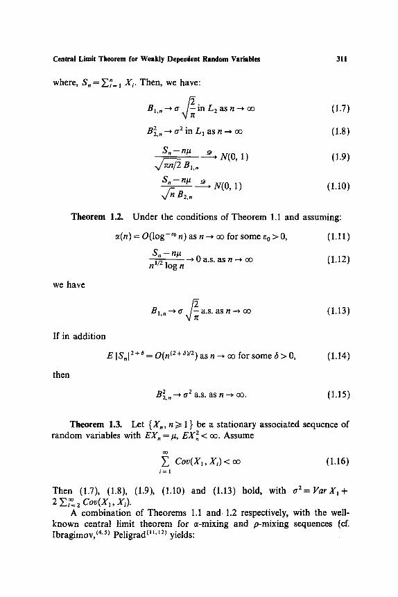
The following theorems give the weak and strong consistency of BI,. to a x / ~ and B22.. to a z, respectively.
Theorem 1.1. Let {X., n/> 1 } be a stationary a-mixing sequence with EX. = 1~, EX2. < oo. Assume
Var S . a2 �9 for some a 2 > 0 as n --) oo
n
S . - n l ~ ,,/-A a , N(O, 1)
(1.5)
(1.6) "
Central Limit Theorem for Weakly Dependent Random Variables
where, S~ = ~,".= l Xi. Then, we have:
Bl,,, --* tr J ~ in L2 as n ~ oo
B22,, --* tr 2 in LI as n ~ oo
S . - n# x / - ~ B,,,, , N(0, 1)
S , , - -n# ~ N(0 ,1 ) x /~ B2,,,
Theorem 1.2.
we have
If in addit ion
then
311
(1.7)
(1.8)
(1.9)
(1.10)
Under the condit ions of Theorem 1.1 and assuming:
ct(n) = O(log-~~ n) as n ~ oo for some s o > 0, (1.11 )
S , - n # , 0 a.s. as n--* oo (1.12) n ~/2 log n
Bl.n-..,,6 a . s . a s n - ~ o o (1.13)
ElS,12+a=O(nC2+~V2)asn--+ooforsome6>O, (1.14)
z~ 2 --+ tr 2 a.s. as n --+ oo. 2, n
Theorem 1.3. random variables with EX, = #, EX2, < az. Assume
(1.15)
Let {X,,, n/> 1 } be a s tat ionary associated sequence of
~Coo(Xl, Xi) < oo (1.16) i = 1
Then (1.7), (1.8), (1.9), (1.10) and (1.13) hold, with t r 2 = V a r X l + 2 E,~2 Cov(X~, x,).
A combinat ion of Theorems 1.1 and. 1.2 respectively, with the well- known central limit theorem for or-mixing and p-mixing sequences (cf. ibragimov,~4,sj PeligradC,.12~ yields:

312 Peligrad and Shao
Corollary 1.1. Let {X,,, n >1 1 } be a stationary a-mixing sequence of random variables with EX, = #, E I X,,12+6 < ~ for some 6 > 0. Assume
~ ~ta/(2+6)(n) < cx3 (1.17) t l = l
Then a2= VarXa+2 ~,i~=2 Cov(X~, "Yi) exists. If in addition tr2>0, then (1.7), (1.8), (1.9), (1.10) and (1.13) hold.
Let {X,, n >t 1 } be a stationary p-mixing sequence of Corollary 1.2. random variables with EX,, = #, EX] < ~ . Assume Var S,, ~ oo and
0(2")<oo (1.18) n = l
Then there exists a positive constant a2 such that
Vat" S, tr 2 * a s n ~ oo (1.19) 1l
Moreover, (1.7), (1.8), (1.9), (1.10) and (1.13) are true. If in addition E [X,,I 2+~ < ov for some & > 0, then (1.15) remains valid.
The proofs of these theorems will be given in the next section, while the proofs of the corollaries are in the Appendix. In Section 3, we will study the convergence rate of (1.7) and (1.8) and establish the corresponding central limit theorem and the law of the iterated logarithm.
2. P R O O F O F T H E O R E M S
We start with some preliminary lemmas.
Lemma 2.1. Let f be a bounded Lipschitz function, i.e.
If(x)l ~< C, for every x (2.1)
I f ( x ) - f ( y ) l <<.F Ix-- Yl for every x, y. (2.2)
Let {X,,,n>>. 1} 'be a stationary e-mixing sequence with EX~=O and EIS , I <~K.n m for some K > 0 and for every n>~l. Then
Vat i~, 7 \--~zJ] <~2C2+32C(1~ FK+C,=,~ (2.3)
for every n/> 1.

Central Limit Theorem for Weakly Dependent Random Variables 313
Proof We have
" l f ( S,'~'~ Var(i~=, 7 \ T J J
1 (~/ / )"s /.@ ( (Si'~,f(Sj'~'~ = ~ -~ Va,'f + 2 ~ Coy f \ 7 , } ~,7] j
i = l i = l j = i + l
: = Ii + I2. (2.4)
It is easy to see that by (2.1), we have:
I, <~ C2 ~ ~ <~ 2C 2 (2.5) i = l
We estimate now 12. Notice that for j > i
coo(i( ,) (s,§
(s,+,,-s2,~
The well-known property of ce-mixing sequence (cf. Davydov (2~') implies
Using (2.1) and (2.2), we obtain
s, s, (s,+2,- ~I(7)(I(7)-I , vq s2')) /%§
<<. 2 C F E IS;+=,- s j - &,l jm < 4CFKit/2 . j- u2
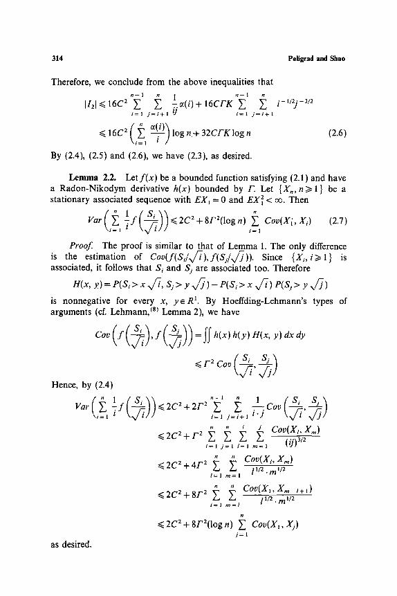
314 Peligrad and Shao
Therefore, we conclude from the above inequalities that
lid ~< 16C 2 ~ =.~(i)+I6CFK i = l j = i + l lJ i = l j = i + I
~< 16C 2 log n + 32CFKlog n i 1
By (2.4), (2.5) and (2.6), we have (2.3), as desired.
i - t/2j - 3/2
(2.6)
Lemma 2.2. Le t f (x ) be a bounded function satisfying (2.1) and have a Radon-Nikodym derivative h(x) bounded by F. Let {X, ,n>~l} be a stationary associated sequence with EXI = 0 and EX~ < oo. Then
Var i = 1 t k x / i / / i=1
Proof The proof is similar to that of Lemma 1. The only difference is the estimation of Cov(f(SJx//7), f(SJx/7)). Since {X~,i>~I} is associated, it follows that Si and Sj are associated too. Therefore
n(x, y)= e(S ,> x x/~, S,> y v / j ) - e ( s i> x x F ) P(S,> y x/~)
is nonnegative for every x, y e R 1. By Hoeffding-Lehmann's types of arguments (cf. Lehmann, r Lemma 2), we have
S i S j
( s , , s , ) <. : cov ./7
Hence, by (2.4)
e l k~/iJJ i=1 i=i+1 l.J
~ i i Cov(Xt, X.,) ~ 2c2 + r ~ ~ Y.
,=, j=, ,=, .,=, (ij) ~/~
g i Cov(X,,X.,) <~ 2C z + 4F 2 lUZ.mU2
I ~ 1 m = l
<.2c2+8r2 coo(x,,xo,_,+,) 1 = 1 m = I l ~/2. m ~/2
~< 2C 2 + 8F2(log n) ~ Cov(X~, Xj) j = l
as desired.

Central Limit Theorem for Weakly Dependent Random Variables 315
Proof of Theorem 1.1. (t.9) and (1.10) are the consequences of (1,6), (I.7) and (1.8). So we only need to prove (1.7) and (1.8). It follows from (1.5) and (1.6) that
E tS,,-nl.t[ x//- ~ + o" as n ~ oo (2.8)
, n >1 1 are uniformly integrable, (2.9)
IX,, - , . I = O( log-2 n) (2.10)
' f . E l--~g n I)7,,- #12 = O( log- ' n) (2.11) i = 1
Therefore, it suffices to show that (1.7) and (1.8) hold with # instead of )7,,. Without loss of generality, we shall assume that # = 0. We shall prove
1 ~ 1 IS,I +trX/~inL2asn~o ~ logn ~=i x//i i
(2.12)
and
1 ~ I S,12 - - ~ a 2 i n L ~ a s n ~ z
log n ,=z21 iz
Let c >t 1 and define the continuous function
(2.13)
I ]0xl if Ixl ~< c,
f(x) := f(c, x) = if Ixl/> c + 1,
{.linear if c < Ixl < c + 1
(2.14)
Clearly, f (x) is bounded by c and has the Lipschitz constant 1 + c. By (2.8) and using Lemma 2.1, we obtain that there exists no independent of c such that for n >/no
ParGo-~ ,=, ~ -~ \---~l,],)
(logn)-Z(2cZ+32c(logn)(2(c+l)(cr+l)+c ~ ~))=0(1) i = l
(2.15)
by the fact that or -~ 0 as n --, co.

316 Peligrad and Shao
We write now:
,_, ;~ -,_,~- 7t tdTS -Ef 1 (Jail f ( S i ~ ( f (S ,~_[S , [~
+,:,~ 7t~- t~j+~t tdTJ dTJJ By using the facts that o<<.lxl-f(x)<<.lxlI{Ixl>~c} and (a+b)~<~ 2a2+ 2b 2 we notice that
E. 1 ~ IS,I - E IS,I 2 ,-~-~.,:, ; -~-
~< 2 Par (1~ ,=l ~ lf(S-~ii))i
+4E(lo-- ~ ~] ~IS~ISlSiI>Ic'~'] z , : , , / ~ t,/7 Js
( ' i '"'s;'/t 's'' }7 +4 ~ , = , 7 .v/7 c.v/7 ~>c ( I ~. l f ( S,'~'~ <~2Var 1--~--~gn,=l 7 \ ~ ] ]
8 " ES ~, c ] , : , -Y- ~ / i
( 1 ~ l f (Si '~ '~ S z" .l'lSil } 2 Var ~ ,:, 7 \ ~ ] / + 8 ,,i-,,,max Ez-~-.'I, i xil~ ~c (2.16)
Now let n ~ ~ first and then c ~ ~ , we conclude that (2.12) holds by (2.16), (2.15) and (2.8). The proof of (2.13) follows the same lines as the proof of (2.12) provided that we use the following function
t O if Ix l~c , g(x) := g(c, x) = if Ixl ~ c + 1,
(.linear if c < Ixl < c + 1.
(2.17)
instead of f (x) . Clearly, g(x) is bounded by c 2 and has the Lipschitz constant 2c. By
(2.8) and using Lemma 2.1, we obtain for every n sufficiently large

Central Limit Theorem for Weakly Dependent Random Variables 317
Var - g iffil i
: = 1
= o(1)
by the fact that ~(n) ~ 0 as n ~ ~ . Noting that
0 <<. x 2 - g ( x ) <<. x 2 I { Ixl/> e}
we have by the same type of arguments as in relation (1.16) that
EIl--~g n l i=1 ~ S~i 2 E(S,. z) ~ < ( V a r ( l o ~ i=, ~" 1-g (S f ) ) )m i ~,~"iJJ]
f ts, I } + 2 max E - ' I >~c
Now let n ~ oo first and then c ~ 0% we conclude that (2.13) holds by (1.5) and the above inequalities.
Proof of Theorem 1.2. We first prove (1.13). Without loss of generality, we assume/z = 0. By (1.12), it suffices to show that
1 1 IS,l_, a . /2 a.s. (2.18) log n x/~ i i = l
Set ck =k 2, n, = [exp(c~/~)] (2.19)
where ~o is as in (1.11). Definef(ek, x) as in (2.14). From '(2.8) and (2.9) it follows that
log n i= l i- x/~ ' a as n ~ ~ , (2.20)
1 .Ef ek, ~cr a s k ~ m, (2.21) log n~ ;= 1
Using Lemma 2.1, by (1.11) and (2.19) we have
Var{ l'---~\log ~ ~ f ck,
16 (c~.+ek(lognk)((l+ck)(l+a)+ck Z ~-~)) i = l
= O(c~ .log-"~ = O(k -4) as k ~ oo (2.22)

318 Pe l ig rad a n d Shao
Noting that log nk + Jlog n k ~ 1 as k ~ oo and applying (2.21), we obtain that for every 0 < e < �88
)i_mP(~ ~ i3,---- T a
~ lira P 1 - - ( 1 - 2 e ) a j~oD j nk--1 i= l i3]2
~< lim ~. p ( 1 ~ IS; l<( l_~,a /~ )
~< lirn ~ P(l~gnki~=,~f(ck, a k=j
+lirn ~ p( I ~ IIS,,I:IS~I>: }>:2a~ ) - k~ ~o-o-o-~;=, 7 ~ i t : ck
~<)im ~. ~ i=l Z f C k,
+lim ~ 4 ~ l_ z~ _ _ lSil .:lSil>~ck 1 j-oo k f jaelognki=l i x/~ [ ~ "9
~<)im ~ 16 ( 1 I f ( S ~ / / ) )
+lim ~. 4 ~ EIS,I ~- j ~ co k = j O'~ log nk i= ~ i2ck
=0
by (2.22), (1.5), and (2.19). This proves that
liminf 1---- .~oo logn i=* /-375~(1 a . s .
and hence
liminr l Z _ ,S,l> . . . . logn i=l / - ~ . t r a . s . (2.23)
Central Limit Theorem for Weakly Dependent Random Variables 319
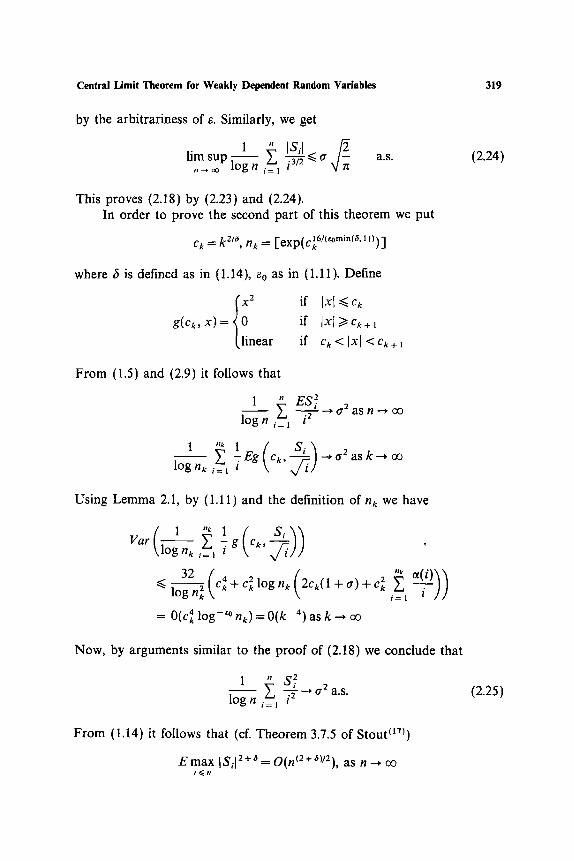
by the arbitrariness of e. Similarly, we get
lira sup ~ /-57i- e a.s. (2.24) n ~ oO i ~ ]
This proves (2.18) by (2.23) and (2.24). In order to prove the second part of this theorem we put
ck = kZ/6,/7 k = [exp(cl6/(~min(& 1)))]
where fi is defined as in (1.14), eo as in (1.11). Define
I O if Ixl ~<Ck g(Ck, X) = if lxl >/Ck + 1
I, linear if Ck<IxI<ck+~
From (1.5) and (2.9) it follows that
1 ~ES~ log n - 7 --* tr2 as n ~ oo
i = l
1 Eg ck, ~ a s k ~ m log n~ i= t
Using Lemma 2.1, by (1.11) and the definition of nk we have
v a t g ck, o i = 1
= 0(c~ log - * ne) = 0 (k -4 ) as k ~ oo
Now, by arguments similar to the p roof of (2.18) we conclude that
1 , l ogn ~=, t-~ -- ~ t r - a ' s " (2.25)
F rom (1.14) it follows that (cf. Theorem 3.7.5 of Stout (17~)
E m a x IS,.12+a = O(nC2+'w2), as n--, m i~<n

320 Peligrad and Shao
Note that
and
and therefore
As a consequence:
IS,,I ISnl ,, ~ o~ ~/2 ~< lim sup max ~/2.. limsUPnU2(logn) k~o~ 2*-~<,<2kn ( logn) 1/2
1 ~< 4 lim sup ~ max ISnl
• P(max IS,,I ~ 2~/2kl/2/log k) k = I n~<2k
<~ ~. (2k/2kl/2/logk) 2+~ E m a x IS,,12§ oo k = 1 n~<2k
1 lim sup ~ max IS,,I = 0 a.s.
k ~ o o 1 . t~. n <~ 2 x
IS,,I lim sup u2 1/2- 0 a.s. (2.26)
. . . . n (log n)
This proves (1.15) by (2.25), (2.26) and (1.4). Now the proof of the Theorem 1.2 is complete.
Proof o f Theorem 1.3. From (1.16) it follows that
Var S,, �9 tr 2 as n ~ oo (2.27) n
and the central limit theorem holds (cf. Newman and Wrightt9)). From the proof of Theorem 1.1, by using Lemma 2.2 instead of Lemma 2.1, we con- clude that (1.7), (1.8), (1.9) and (1.10) hold. To finish the proof of (1.13), similarly to the proof of Theorem 2.2, we only need to verify (1.12). In terms of the maximal inequality (cf. Newman and WrighttgJ), we have
2 liar S________~,, P(max I S i - ES~I >1 x + 2 ~ S,,) <<.
i ~ n X 2
Similarly to the proof of (2.26), we have
1 lim sup IS, - npl/(n u2 log n) ~< 4 lim sup --7=-.- max IS,, - n/~l
_ 2 ~/zl- n ~ o o n ~ o o I~ n <~ 2 k
Central Limit Theorem for Weakly Dependent Random Variables
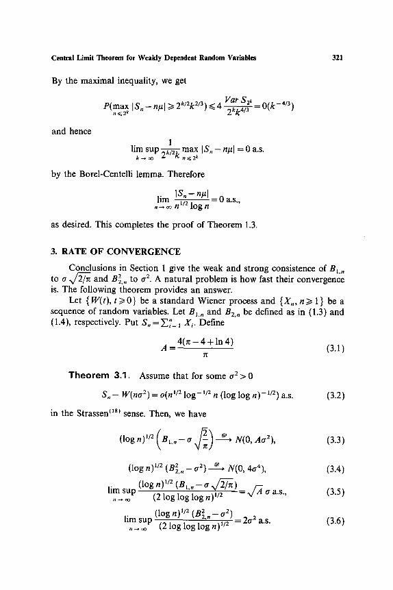
By the maximal inequality, we get
Vat $2, P(max IS. - n#l f> 2k/2k 2/3) <~ 4 2kk4/3 -- O(k -4/3)
n <~ 2 k
and hence 1
lim sup 2-~-~k max IS,,-nl~l =0 a.s. k ~ c t ~ n~<2 k
by the Borel-Centelli lemma. Therefore
lim ~ = 0 a.s., , , - ~ n log n
as desired. This completes the proof of Theorem 1.3.
321
3. RATE OF CONVERGENCE
Conclusions in Section 1 give the weak and strong consistence of B~,, to 0. x / ~ and B~.,, to 0.2. A natural problem is how fast their convergence is. The following theorem provides an answer.
Let { W(t), t >>. 0} be a standard Wiener process and {X,, n >/1 } be a sequence of random variables. Let BL, and B2,n be defined as in (1.3) and (1.4), respectively. Put S,, = Z~'= 1 Xi. Define
4(n -- 4 + In 4) A = (3.1)
T h e o r e m 3.1. Assume that for some 0.2>0
S , , - W(n0. 2) = o(n 1/2 log-u2 n (log log n)-1/2) a.s. (3.2)
in the Strassen c.8~ sense. Then, we have
( logn) ' /2(B, . , , -0. / ~ ) ~ , N(O, A0.2), (3.3)
(log n) m 2 ( B 2 , n - - 0 "2) , N ( 0 , 4 0 .4 ) ,
lim sup (log n) u2 (BI. , ,- 0. ~/2/rc) ~ x / ~ 0. a.s., . . . . (2 log log log n)u2
(log n) 1/2 2 ( B 2 , n - - 0. 2 ) lim,,~sup~o (2 log log log n) 1/2 - 20.2 a.s.
(3.4)
(3.5)
(3.6)

322 Peligrad and Shao
Applying Theorem 3.1 to s tat ionary 0t-mixing and p-mixing sequences, we obtain
Corollary 3.1. Let {X,,, n>_-1} be a stat ionary 0t-mixing sequence with EX,, = 0 and E IX,,12+6 < oo for some t5 >0 . Assume
2 + 6 ~(n) = O(n-r) for some y > - - (3.7)
Then a 2 = EX~ + 2 Z~=2 EX1Xi exists and (3.3), (3.4), (3.5) and (3.6) hold if a 2 > 0 .
Corollary 3.2. Let {X~, n>~ 1 } be a s tat ionary p-mixing sequence with . E X , = 0 and E]X,,]2+n<oo for some di>0. Assume ES2~oo as n ~ oo and
p(n) = O(log - r n) for some y > 2
Then there exists or2> 0 such that
(3.8)
ES~ �9 ~2 n
and (3.3), (3.4), (3.5) and (3.6) hold.
Proof of Theorem 3.1. Let {W(t), t~>0} process. Write
Because
W - 1 ~ I W(ia2)[ ~'" - log n i= ~ i3/2
1 ~ W2(io "2) W2 " = l~ n i=1 , i2
be a s tandard Wiener
(3.9)
(3.10)
1 " ]W(i t r2) l - IS,[ 1 ~. 1 IS, I
Then
(log n) 112 [ WI,~, I - Bl,nJ
2 IS.I n ~/2+ 1 ~. I S i - W(iaz)l ~< ~ ( l o g ) (log n) 1/2 i= 1 i3/2

Central Limit Theorem for Weakly Dependent Random Variables 323
Because
I W2,, 2 1 ( ' ~ W2(itr2)--S2 ~ IS;IIS, I S~.~) " - B 2 ' " I < ~ , i - : + 2 - +
i = l l n
we have
(log n) 1/2 I W2.,,- 2 Bz,,I
1 ( ' ~ = ISi-W(itr2)l.(ISil+l " ]S,I ~ ~ ) (logn) 1/2 i 1 n J=l
i2 W(ztr2)l ) + 3
Therefore, under the assumption of Theorem 3.1,
(log n )~/2 I WE, - B1.,, I = o( i ) a.s. (3.11 )
( log/ , / )1/2 I W2,n - - B2,,I = o(1 ) a.s. (3.12)
Thus, Theorem 3.1 will immediately follow as a consequence of the following auxiliary result:
T h e o r e m 3.2. have, for tr 2 > 0:
( 1 ~ IW(ia2)l N/~ ) (log n ) 1/2 ~ i3/2 t~
i = l
(l~ ~ i = 1 i2 0"2
Let { W(t), t >/0} be a standard Wiener process. We
~, N(0, A o "2) (3.13) t
~, N(0, 4tr 4) (3.14)
(log n)1/2 lim,,_supco (2 log log log n ) 1/2
X i3/2 i = l
o" ~ ) = A 1/2o" a.s., (3.15)
(log n) 1/2 lim sup
.~oo (2 log log log n) z/2
x 1 W2(itr 2) _ cr2~ = 2a 2
/ i = l a.s., (3.16)
860p/2-8

324 Pel ig rad and SIlao
. . r f l o g log log n~l/z l m i n l / - - - .~o~ \ l o g n /
• ~ ] W ( i o ' 2 ) l - . ~ t r x / ~ = 7r A j<~n i = l i3/- x//- ~ l/2tr a.s., (3.17)
lo ) 'n ( l o g l o g g n lim inf
. ~ o~ /,, log
x max - - = J~<" i= : i2 I
We start with some lemmas, whose proofs will be given in the Appendix.
L e m m a 3.1. Let X and Y be independent s tandard normal r a n d o m variables. Then
C~ 2 ( ~ ) = - a - ~/1 + a 2 + arcsin rc
for every a/> 0.
(3.19)
L e m m a 3.2. Let X and Y be two s tandard normal r a n d o m variables and joint ly no rma l with p = EXY>~ O. Then
Coo(IXI, IYI)=2Prr a r c s inp 1 + (3.20)
L e m m a 3.3. Let {W(t),t>>.O} be a s tandard Wiener process. We have
: I W(e')[ Vat e,/----- T - dt = A T+ O(log T) (3.21)
ro W2(e') dt O(1) (3.22) Vat e---- T - = a T +
as T--* oo, where A = 4 ( T r - 4 + l n 4)/n, as in (3.1).
L e m m a 3.4. Let { W(t), t 1> 0} be a s tandard Wiener process. Deno te Y( t ) = W( e')/e 1/z', t >>. O. Then { Y( t ), t >>. 0} is a s ta t ionary p-mixing process with
p(v) = O(e -~/4) as v ~ oo (3,23)

Central Limit Theorem for Weakly Dependent Random Variables 325
Proof of Theorem 3.2. Since { W(ta2). t>~0} and {aW(t). t~>0} have the same distribution, without loss of generality, we can assume tr = 1. We first show (3.13), (3.15) and (3.17). Put
T. := ~ ]W(i)I-EI:W(i)I i 3/z (3.24)
i = l
T,, := j~r "lW(t)t-EIW(t)lt- ~ dt _ f'"" W(e')FI-EFW(e")Ie,:2 dt - -r
(3.25)
Notice that ( 1 ~ [W�91 ~/~)
(log/,/)1/2 [ - ~ g n i 3/2 i i = l
- (log--n)'/2 + (log n) / ~.,~ ~ , = , 7 -
T'. O((log n)-1/2) - (log n)l/2 +
IT=- :F.I ~< I W(1)I + E I W(1)I
and
i = 2 ( [ W ( i ) I - E I W ( i ) [ ) i~/2 t~/2
+ ,=~2 f:-xlW(i)[:--[W(t)[--E"llW~i')~l;+ElW(t)lt3/2 dt I'
~IW(1)I-1-EIW(1)I + ~ (IW(i)1-1-E IW(i)l)) i = 2
5 I 2. (,i ~ 1 )5/2
• f ' supo,~, ~, I w ( i ) , - w ( i - s)l + 1 -1- t3/2
i=2 --1 dt
~<16+12 ~ [W(i)I i= I i5/2
'~i 2 f; S U p o ~ ]W(i+s-1,)-W(,i-1)~ld t + , i - 1 t 3/2
oo l w(ol ~< 16 + 12 i= 1 is~2
(3.26)
~. I w(i)l i= ~ is/2
---§ ~ SUpo~,~<~ l'W(,i+s):- W(.i)I i3/2 < oo a.s. (3.28)
i = l
- - - t - 8 ~ SUPo~<s~<l ]W(i+s)~--W(i)] i3/2 (3.27)

326 Peligrad and Shao
by the fact that ~.~~ Z;~176 i Esupo~s~ ~ I W(i+ s ) - W(i)l/i 3/2 <CX3.
Therefore IT,,-:rl <oo a.s. By (3.26)-(3.28) and by taking into account that
, l o g n ) ~ / 2 ( l o _ ~ l W ( i , I ~__~ T,, ( 1 ) ,=1 i3 / z ~/~] = ~ , / 2 I- 0 -(logn),/~ a.s.
in order to prove (3.13) and (3.15) it suffices to show that
(log n) m , N(O, A)
T- = x/-~ a.s" lim,_.oosup (2 log n. log log log n) 1/2
(3.29)
(3.30)
In order to prove (3.17), because
J I W ( i ) l - x / ~ x / ~ max ~ 7 ~ = max ITjl = max ILl + o(1) a.s. j<~n i 1 j<~n j<~n
it is enough to establish
. . ~ f log log log n'~ 1/2 7z l m l n I , - - ./ max i~il=.___=x/Aa.s . r - 7 . . oo \ l og n ] i~, . ,/8
Put
(3.31)
' I W(e')l - g I W(e')[ ~k = e,/2 dt,
--1
b, = E ~,- k = 1, 2 .... i 1
Then, by Lemma 3.4, {~k,k>~ 1} is a stationary p-mixing sequence with E ~ , = 0 , Elr for every p > 0 and with p-mixing rate p(n) = O(e-(1/4)n). Applying a strong approximation theorem of Shao, t~4) without changing the distribution of {~k,k~>l}, we can redefine { ~k, k >_- 1 } on a richer probability space together with a standard Wiener process { W(t), t >>. O} such that
• r W(b,) = O(n 1/2 log -4 n) a.s. (3.32) i = l
Central Limit Theorem for Weakly Dependent Random Variables 327
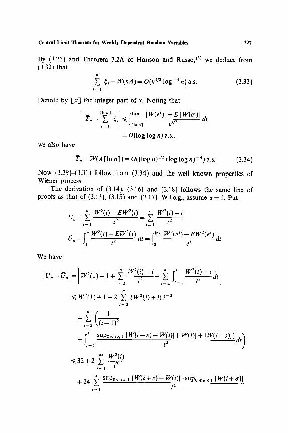
By (3.21) and Theorem 3.2A of Hanson and Russo, (3) we deduce from (3.32) that
~ r W(nA)= O(/l 1/2 log -4 n) a.s. (3.33) i ~ l
Denote by Ix] the integer part of x. Noting that
T, , - t ~ l G ~< |c'"" I W(e')l + E lW(e')l dt i = 1 dl-ln n] e t/2
= O(log log n) a.s.,
we also have
7",,-W(A[lnn])=O((logn)UZ(loglogn)-4)a.s. (3.34)
Now (3.29)-(3.31) follow from (3.34) and the well known properties of Wiener process.
The derivation of (3.14), (3.16) and (3.18) follows the same line of proofs as that of (3.13), (3.15) and (3.17). W.l.o.g., assume ~r = 1. Put
W2(i) - EW2(i) ~ W2(i) - i U,, L
i = 1 i = 1
~r = f" W2(t)-- EW2(t) dt = fin, W2(e')-- EW2(e ~) -~ ~o e t d 1
dt
We have
IU, , - 0.1 = w 2 ( 1 ) - 1 + i2 t2 i = 2 i = 2 --1
~<W2(1)+1+2 Z (WZ(i)+i)i -3 i = 2
+ (i--1)2 i = 2
f; sup~<,~<~ l W(i--s)-- W(i)! (1W(i)J + I W(i--s)l) dt) + t 2 - -1
~<32+2 i3 i = l
+24 ~ supo~<~<~ [W(i+s)-- W(i)[ "sup0~<,<~t [W(i+a)l i 2

328 Peligrad and Shao
and
( ~ W2(i) ~ SUpo~<=~<, lw(i+s)-W(i)l .supo, , .~, IW(i+v)l) E ~ + i2
\ i = 1 i = 1
(i + 1)u2. (E supo~<s~< I I W(s)12) In" (E supo~<,.~< 1 I W(v)12) m +
i 2 i = 1
Therefore
lim sup [U,, - 0,,I < ~ a.s." # t ~
Because
w2,,,) ( 1 ) (log n) '- t ~ ~ i 2 1 - (log n)l/2 + 0 (log n)i'2 a.s.
i = 1
in order to prove (3.14), (3.16) and (3.18), it suffices to show that
(log n) m > N(0, 4)
lim,,_supoo (2 log n log log log l'1) 1/2 = 2 a.s.
(3.35)
(3.36)
lim inf ( l~ l~ l~ n) m 2~88 max loll = a.s. . . . . log n J i~,,
(3.37)
Put
' Wz(e') - EWZ(e ') qk = e' dt
- - t
_ , , , , , e i t e,/~ ) ) d t
c , = E tl~ , k = l , 2 .... i 1

Central Limit Theorem for Weakly Dependent Random Variables 329
By the same arguments leading to (3.32) and (3.33) we have
~, ~]i-- W(cn ) = O( hI~2 l o g - 4 n) a . s .
i=1
~ q i - - W(4n) = O(n t/Z log--4 F/) a.s. i = l
Noting that
rlog,,l [ f ' "" WZ(e')+EWZ(e')at 0, . - Z 'I, <~"ct.,,l e'
i=1
= O((log log n) 2) a.s.
by the law of the iterated logarithm, we also have
~ ' , , - W(4[ln n]) = O((log n) 1/2. (log log n) -4) a.s.
(3.38)
(3.39)
in the Strassen sense. The conclusions now follow immediately from Theorem 3.1.
Proof of Corollary 3.2. By Theorem 1 of Bradley, t~) we have
ES~ ~ cr 2 for some e2 > O, as n --* oo n
and there exist positive constants C and D such that for all n/> 1
I1 i = 0
by (3.8). A strong approximation theorem of Shao tl4~ shows
S,, - W( ES ~) = O(nl/2(log n) - ~ - iv2)) a.s.
(3.41)
(3.42)
(3.43)
Now (3.35)-(3.37) follow from (3.40) and the well-known properties of the Wiener process.
Proof of Corollary 3.1. It is well-known that tr 2 exists under condi- tion (3.15). If in addition o2>0, then, by Theorem4 of Kuelbs and Philipp ~7) (cf. Shao, ~ Th. 5.2.4), we have
S , , - W ( n ~ 2 ) = O ( n v2-~') a.s. for some 2 > 0
(3.40)

330 Peligrad and Shao
A combination of (3.42), (3.43) together with Theorem 3.2A of Hanson and Russo (3) yields.
Sn __ W ( n t r 2 ) = O(nUZ(log n)-tr-1)]2 (log log n ) 1/2) a .s . (3.44)
Therefore, (3.2) is satisfied. Now Corollary 3.2 is a direct consequence of Theorem 3.1.
Remark 1. We suspect that a direct approach of Theorem 3.1 is possible but it will involve tremendous computation; so we are not going to present it here.
4. APPENDIX
Pt:oof o f Corollary 1.1. It is well known Oodaira and Yoshihara, ~t~ and Peligrad t12~)
Var S,, tr 2 -,. a s n ~ /,/
that (cf. Ibragimov, t4)
and (1.6) holds if cr 2 >0. Hence by Theorem 1.1, the relations (1.7), (1.8), (1.9) and (1.10) hold. To prove (1.13), by Theorem 1.2, it suffices to show that (1.12) is satisfied. Without loss of generality we assume g = 0 . Applying Lemma 1 of Shao, t~s) we get
P(max ISil >>. x) <<. 4 nE IX111{(x,I ~ C} +4+ i~< n X X
(32) 3 nC~(m) (4.1)
for any x >/1, c > 0 and integer m satisfying
x and n( E IXl l 2 + ~) 2/~2 + ~) ~ ct~/t2+~)(i)~<
x 2 (4.2)
1 ~< m ~< 64C log x i=0 (32) 3. log x
For a given arbitrary 0 < e < 1/32, put
n k = 2 k, x = enlk/2 log n k , C = n~/t2tl +~)), m = [n~ It2~ +6))]
It is easy to see that (4.2) is satisfied by (1.17), provided k is sufficiently large. Using (4.1), we obtain
4nkE [X,[ I{[Xll f>rt~/(2(1 + ~))} P(max [S;[ t> en~/z log nk) ~<
i<.,, en~/2 log nk
4 (32)3. n~/2+ l/t2ta + a))~(m) + (4.3)
q- enlk/2 log//k e log nk
Central Limit Theorem for Weakly Dependent Random Variables 331
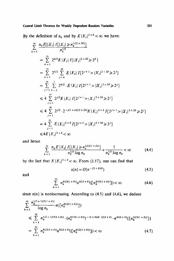
By the definition of nk and by E IX~[ 2+a < c~ we have:
(--, m,g(IX~l I{IX~I >~n~/(2+z~)} k/-'= t nff 2
and hence
= ~ 2k/ZEIX, II{IX,12+2~>~2 k}
= ~ 2 */2 ~ EIX, II{2J+x>IX~I2+Za>~2 j} k=l j = k
i ' = y. 2~a.EIX, II{2J+~>IX,12+2o>~2 j}
j = l k = l
<~ 4 ~ 2J/~E IX~I I {U § > Ix~l ~+~ >t 2Q y = l
<~ 4 ~ 2 j/2 .2-J( t+a)/ (2+2'DE IX, I 2+~ 1{2 y+~ > IX~lZ+2a>~2J} j = t
= 4 ~ EIXll2+~I{2-i+l> IX~12+2~>~2 ~} . t ' = t
~<4E IX~l ~§ <
~,, nkE lX, l I{IXd ~>n# ~m+a'} 1 k = t n 1/2 log ne + nlk/2 log n k < oo (4.4)
by the fact that E IXl l2+a< oo. From (1.17), one can find that
or(n) = O(n -~2 +'~/~) (4.5)
and
. . a / ( 2 r + a ) ) : a / ( 2 + a)? F~,a/(2(1 + a ) ) - I ) < oO (4.6) k = l
since 0t(n) is nonincreasing. According to (4.5) and (4.6), we deduce
k = ~ log nk
k = l
n~/(m+~))~~176176 < oo (4.7) k = l
332 Peligrad and Shao
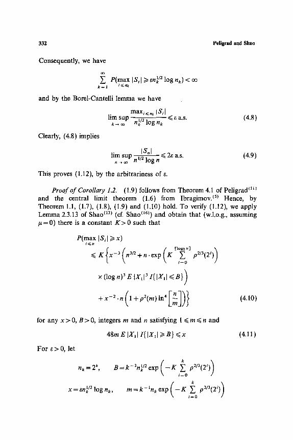
Consequently, we have
Z P(max ISil >1 en~/2 log nu) < oo k = l i<~ltk
and by the Borel-Cantelli lemma we have
maxi~<,,k [Sil lim sup ~< ~ a.s. (4.8)
k ~ o~ ntk/2 log nk
Clearly, (4.8) implies
ISnl lim sup - - ~< 2~ a.s. (4.9) n-,oo nl/21ogn
This proves (1.12), by the arbitrariness of 5.
Proof of Corollary 1.2. (1.9) follows from Theorem 4.1 of Peligrad r and the central limit theorem (1.6) from Ibragimov. ~5) Hence, by Theorem 1.1, (1.7), (1.8), (1.9) and (i.10) hold. To verify (1.12), we apply Lemma 2.3.13 of Shao ~3) (cf. Shao ~t6j) and obtain that (w.l.o.g., assuming # = 0 ) there is a constant K > 0 such that
P(max ISil >~ x) i~<n
i = 0
x (log n) 3 E IXll 3 I{ IX~I ~ B})
+ x - 2 . n ( l + p 2 ( m ) l n 4 I n l ) } (4.10)
for any x > 0, B > 0, integers m and n satisfying 1 ~< m ~< n and
48m E IXjl I{IXll >/B} ~<x
For e > 0, let
i = 0
x=en~/210gnk, m = k - i n k e x p --K ~. p2/3(2i) iffiO
(4.11)
Central Limit Theorem for Weakly Dependent Random Variables 333
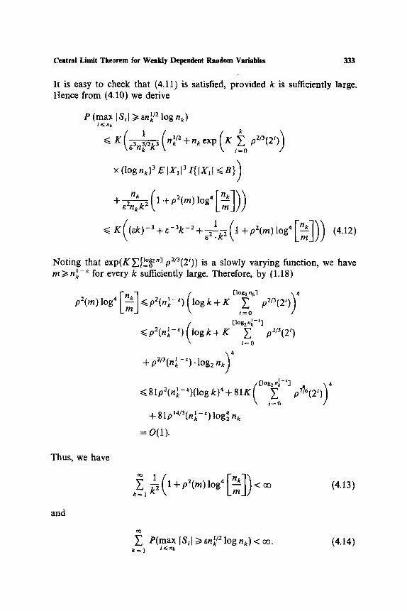
It is easy to check that (4.11.) is satisfied, provided k is sufficiently large. Hence from (4A0) we derive
P (max IS, I >18n~/2 log nk) i~nk
K 1 k
x (log nk) 3 E IX~l 3 l{ IXll ~< B } )
+ ~ (1 + P2(m) l~ [ ~ ] ) )
<~ K((~k)-3+e-3k-2+ 21~.k2(t+o2(m)log'l[~]) ) (4.12)
Noting that exp(K~ft~~ 2"J p2/3(2i)) is a slowly varying function, we have >. n 1-4 for every k sufficiently large. Therefore, by (1.18)
[Iog2 n l - r ] / (log k + K E \ i ~ 0
+ pz/3(nlk- ~)" log2 nk) 4
t" [log 2 nk I-r ']
<~ 81p2(n~-")(logk)4 +81K I i~r
+ 81p14/3(n~ -~) log~ nk
[log 2 n k] / 4 ~, p2/3(2')
i~O
p~/3(2")
= O(1).
p7 /6 (2 i
Thus, we have
k= 1 ~-/ 1 + p2(m) log 4 < oo (4.13)
and
• P(max IS~l 1> en~/2 log nk) < o0. k ~ l i~nk
(4.14)

334 Peligrad and Shao
Now (1.12) immediately follows from (4.14). (cf. (4.9)). Hence (1.13) holds. If in addition E IXll2§ oo for some 6 >0, then (1.14) is satisfied by (1.19) (of. Ibragimov tS)) and (1.15) follows from Theorem 1.2. This completes the proof of Corollary 1.2.
Proof of Lemma 3.1. We have
EIXI IX+aYI =~--~ - ~ . -oo Ix2+axyl e-(X2+Y2)/2dxdy
= ~ Icos'- 0 + a cos 0 sin 01 dO 73e-~2/2 d~
1 f]~ ]cos 2 0 + a cos 0 sin Ol dO (4.15)
Write
a ~ m 7~ cos ~o where 0 < r ~<
sin q~'
Notice that
f0 Ic~ 0 + a cos 0 sin 01 dO = ~ Jo Icos 0- sin(q~ + 0)1 dO
_ 1 f ~ Isin(q~ + 20) + sin r dO 2 sin ~o
fo = 1 Isin(tp+20)+sin~oldO sin ~o
'(;? - sin ~o (sin(q~ + 20) + sin q~) dO
- f ~ - ~ (sin(~o + 20) + sin tp) dO /2
) + (sin(~o + 20) + sin q~) dO
( 1) = 2(r + a ) = 2 a + arcsin ~ (4.16)
A combination of (4.16) with (4.15) yields (3.19)
Central Limit Theorem for Weakly Dependent Random Variables 335
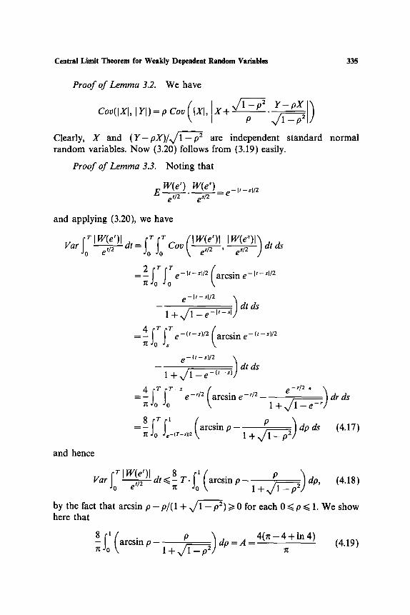
Proof of Lemma 3.2. We have
Coo(IXI, IYI)--p Cov(IXl, x+ ~/T-p2 Y-py
Clearly, I" and ( Y - pX)/x/1 - p2 are independent standard random variables. Now (3.20) follows from (3.19) easily.
Proof of Lemma 3.3. Noting that
normal
E W(e') W(e s) _ _ _ _ ~ _ e - l t - s l / 2 e t/2 eS/2
and applying (3.20), we have
liar ~ I W(e')let/2
and hence
[-olo (IW(e') lIW(e~)l) - - dt = Coo e,/2 , e,/Z dt ds
=2frfroe-, , - , , /2(arcsine-, , -~, /2
- e-"-"/2 .~dtds 1 + x / 1 - e - I ' - s l J
4 f r f r _ (,- ~)/2 (arcsin e - ( ' - s)/2 =~Jo %. e
e - ( t - s ' / 2 .'~
1 + x/1 --e -('-~)] dt ds
=~4 [rlr-~oo o e-r/2 ( arcsin e - r /2-
8 I "r ~1 [ . = - J. j /arcsm p
7[ 0 e -(T-s)/2 \
e - d 2 �9
1+ ~ / dr ds
,4.17,
r I W(e')l dt <8 T. arcsin p P dp, (4.18) Var eU 2 rc 1 +
by the fact that arcsin p-p~(1 +~/1 -p2)>~O for each O~<p~< 1. We show here that
8 ~ ( plx~_p2) dp=A 4 ( n - 4 + l n 4) (4.19) arcsin p 1 + -

336 Peligrad and Shao
Write p = sin 0. We find
l( l + ~ P ) _f~/2( sin0 ) f0o arcsin p - dp 0 cos 0 dO
- . 0 1 +cos 0
:? =Osin 0[; /2- sinOdO
~ /2 fo/2 sin 0 - sinOdO+ - - d O
-o 1 + cos 0
= - - 2-1n(1 +cos 0)tg/2 2 1
= ~ (:~--4+ln 4)
as desired. A combination of (4.18) with (4.19) yields
yo I W(e')l Var #/2 dt <~ A T for every T > 0 (4.20)
On the other hand, by (4.17), we have
frlW(e')l Var e,/----W-- - dt
8 T-- 2 log p - arcsin p - dp ds f -(T--~)/2 n-o 1+
t> - (T- 2 log T) arcsin p dp n ~/r 1 +
~> ~ ( T - 2 1 o g T) arcsin p-- 1 + ~ alp-
>t A T - 8 log T - 6
by (4.19). This proves (3.21) by (4.20) and (4.21). We next prove (3.22). Notice that
Io W2(e')dt ~ o ~ (W2(e')W2--~es))dtds Far e' = 2 Coo e' '
= 2 ~o f f Var W2(e')e,+, dt ds
T T
= 4 f o r e-"-S)dtds
=4(T- - 1 + e -r) This proves (3.22).
(4.21)

Ce~ntrai Limit Theorem for Weakly Dependent Random Variables 337
Proof o f Lemma 3.4. Clearly, { Y(t), t/> 0} is an Orns t e in -Uh lenbeck process, a s t a t iona ry Gauss i an process with covar iance funct ion
Coy( Y(t + p), Y(t)) = e-U/2 for each t, # >t 0
and the spectral densi ty
l j ' ? d # = (1 2 = - e -~'/2 cos(X#) f (X) rr + 4X 2)
= L - 2 ( X ) ,
where L ( X ) = x/rr(1 + 422)/2. I t is easy to see tha t
(i) S ~ In IL(X)[/(1 + 2 2 ) d X < oo,
(ii) L(X) has two nonrea l zeros zl = i/2 and z2 = - i / 2 ,
(iii) sup_oo<~,<oo ( l l , , , (1 / (X-z , ) ) l + [I , , , (1 / (X-zz)) l ) = sup_ ~o < ~.< o~ 4/(1 + 4X 2) = 4.
Therefore, by [ I b r a g i m o v and Rozanov /6 ) T h e o r e m 6 , { Y(t), t >/0} is a s t a t ionary p-mix ing process with
p ( z ) = O ( e -"' /2-~1) as z o ao for each ~ > 0 .
p. 217] ,
(4.22)
In par t icu lar , we have (3.23).
A C K N O W L E D G M E N T
The au thors thank Jeesen Chen for his help in the p r o o f of L e m m a 3.1. Thanks also to the referee for his va luable comments .
REFERENCES
1. Bradley, R. C. (1981). A sufficient condition for linear growth of variances in a stationary random sequence, Proc. Amer. Math. Soc. 83, 586--589.
2. Davydov, Yu A. (I970). The invariance principle for stationary processes, Th. Prob. AppL 15, 487-498.
3. Hanson, D. L. and Russo, P. (1983). Some results on increments of the Wiener processes with applications to lag sums of i.i.d, random variables, Ann. Prob. 11, 609-623.
4. Ibragimov, I. A. (1962). Some limit theorems for stationary processes, Th. Prob. Appl. 7, 349-382.
5. Ibragimov, I. A. (1975). A note on the central limit theorem for dependent random variables, Th. Prob. Appl. 20, 135-141.
6. Ibragimov, I. A. and Rozanov, Y. A. (1978). Gaussian Random Processes, Springer-Verlag, New York.
7. Kuelbs, J, and Philipp, W. (1980). Almost sure invariance principles for partial sums of mixing B-valued random variables, Ann. Prob. 8, 1003-1036.
338 Peligrad and Shao
8. Lehmann, E. L. (1966). Some concepts of dependence, Ann. Math. Statist. 37, 1137-1153. 9. Newman, C. M. and Wright, A. L. (1981). An invariance principle for certain dependent
sequences, Ann. Prob. 9, 671-675. I0. Oodaira, H. and Yoshihara, K. (1972). Functional central limit theorems for strictly
stationary processes satisfying the strong mixing condition, Kodai Math. Sere. Rep. 24, 259-269.
11. Peligrad, M. (1982). Invariance principles for mixing sequences of random variables, Ann. Prob. 10, 968-981.
12. Peligrad, M. (1986). Recent advances in the central limit theorem and its weak invariance principle for mixing sequences of random variables, in: Dependence in Probab. and Statist., Eberlein, E. and Taqqu, M.S. (eds.), Progress in Prob. and Statist. 1I, 193-223.
13. Shao, Q. M. (1989). Limit theorems for sums of dependent and independent random variables, Ph.D. Dissertation, University of Science and Technology of China, Hefei, P.R. China.
14. Shao, Q. M. (1991). Almost sure invariance principles for mixing sequences of random variables, Tech. Rep. Ser. Lab. Res. Stat. Probab. No. 185, Carleton University. University of Ottawa, Ottawa. Stochastic Process. AppL (to appear).
15. Shao, Q. M. (1993a). Complete convergence for ~-mixing sequences, Prob. Statist. Lett. 16, 279-287.
16. Shao, Q.M. (1993b). Moment and probability inequalities for partial sums of p-mixing sequences. Research Report No. 556, Department of Mathematic, National University of Singapore.
17. Stout, W. F. (1974). Almost Sure Convergence, Academic Press, New York. 18. Strassen, V. A. (1964). An almost sure invariance principle for the law of the iterated
logarithm, Z. Wahr. Verw. Gebiete 3, 211-226.