Black Box Absolute Reconstruction for Sums of Powers ... - arXiv

arX

iv:2

110.

0530

5v1

[cs

.CC

] 1

1 O

ct 2

021

Black Box Absolute Reconstruction

for Sums of Powers of Linear Forms

Pascal Koiran and Subhayan Saha∗

Abstract

We study the decomposition of multivariate polynomials as sumsof powers of linear forms. We give a randomized algorithm for the fol-lowing problem: If a homogeneous polynomial f ∈ K[x1, ..., xn] (whereK ⊆ C) of degree d is given as a blackbox, decide whether it can bewritten as a linear combination of d-th powers of linearly independentcomplex linear forms. The main novel features of the algorithm are:

• For d = 3, we improve by a factor of n on the running time fromthe algorithm in [KS20]. The price to be paid for this improve-ment though is that the algorithm now has two-sided error.

• For d > 3, we provide the first randomized blackbox algorithm forthis problem that runs in time poly(n, d) (in an algebraic modelwhere only arithmetic operations and equality tests are allowed).Previous algorithms for this problem [Kay11] as well as most ofthe existing reconstruction algorithms for other classes appeal toa polynomial factorization subroutine. This requires extractionof complex polynomial roots at unit cost and in standard modelssuch as the unit-cost RAM or the Turing machine this approachdoes not yield polynomial time algorithms.

• For d > 3, when f has rational coefficients (i.e. K = Q), therunning time of the blackbox algorithm is polynomial in n, d andthe maximal bit size of any coefficient of f . This yields the firstalgorithm for this problem over C with polynomial running timein the bit model of computation.

These results are true even when we replace C by R. We view the prob-lem as a tensor decomposition problem and use linear algebraic meth-ods such as checking the simultaneous diagonalisability of the slices of atensor. The number of such slices is exponential in d. But surprisingly,we show that after a random change of variables, computing just 3 spe-cial slices is enough. We also show that our approach can be extendedto the computation of the actual decomposition. In forthcoming workwe plan to extend these results to overcomplete decompositions, i.e.,decompositions in more than n powers of linear forms.

∗Univ Lyon, EnsL, UCBL, CNRS, LIP, F-69342, LYON Cedex 07, France. Email:

[email protected].

1

http://arxiv.org/abs/2110.05305v1

1 Introduction

Lower bounds and polynomial identity testing are two fundamental prob-lems about arithmetic circuits. In this paper we consider another funda-mental problem: arithmetic circuit reconstruction. For an input polynomialf , typically given by a black box, the goal is to find the smallest circuitcomputing f within some class C of arithmetic circuits. This problem canbe divided in two subproblems: a decision problem (can f be computedby a circuit of size s from the class C?) and the reconstruction problemproper (the actual construction of the smallest circuit for f). In this pa-per we are interested in absolute reconstruction, namely, in the case whereC is a class of circuits over the field of complex numbers. The name isborrowed from absolute factorization, a well-studied problem in computeralgebra (see e.g. [CG05, CL07, Gao03, Sha09]). Most of the existing re-construction algorithms appeal to a polynomial factorization subroutine,see e.g. [GMKP17, GMKP18, KS09, Kay11, KNST18, KS19, Shp09]. Thistypically yields polynomial time algorithms over finite fields or the field ofrational numbers. However, in standard models of computation such as theunit-cost RAM or the Turing machine this approach does not yield polyno-mial time algorithms for absolute reconstruction. This is true even for thedecision version of this problem. In the Turing machine model, the diffi-culty is as follows. We are given an input polynomial f , say with rationalcoefficients, and want to decide if there is a small circuit C ∈ C for f , whereC may have complex coefficients. After applying a polynomial factorizationsubroutine, a reconstruction algorithm will manipulate polynomials with co-efficients in a field extension of Q. If this extension is of exponential degree,the remainder of the algorithm will not run in polynomial time. This pointis explained in more detail in [KS20] on the example of a reconstruction algo-rithm due to Neeraj Kayal [Kay11]. One way out of this difficulty is to workin a model where polynomial roots can be extracted at unit cost, as sug-gested in a footnote of [GGKS19]. We will work instead in more standardmodels, namely, the Turing machine model or the unit-cost RAM over C

with arithmetic operations only (an appropriate formalization is providedby the Blum-Shub-Smale model of computation [BCSS98, BSS89]). Beforepresenting our results, we present the class of circuits studied in this paper.

1.1 Sums of powers of linear forms

Let f(x1, . . . , xn) be a homogeneous polynomial of degree d. In this paperwe study decompositions of the type:

f(x1, . . . , xn) =r

∑

i=1

li(x1, . . . , xn)d (1)

2

where the li are linear forms. Such a decomposition is sometimes called aWaring decomposition, or a symmetric tensor decomposition. The smallestpossible value of r is the symmetric tensor rank of f , and it is NP-hard tocompute already for d = 3 [Shi16]. One can nevertheless obtain polynomialtime algorithms by restricting to a constant value of r [BSV21]. In this paperwe assume instead that the linear forms li are linearly independent (hencer ≤ n). This setting was already studied by Kayal [Kay11]. It turns out thatsuch a decomposition is unique when it exists, up to a permutation of the liand multiplications by d-th roots of unity. This follows for instance fromKruskal’s uniqueness theorem. For a more elementary proof, see [Kay11,Corollary 5.1] and [KS20, Section 3.1].

Under this assumption of linear independence, the case r = n is ofparticular interest. In this case, f is equivalent to the sum of d-th powerspolynomial

Pd(x) = xd1 + xd

2 + · · · + xdn (2)

in the sense that f(x) = Pd(Ax) where A is invertible. A test of equivalenceto Pd was provided in [Kay11]. The resulting algorithm provably runs inpolynomial time over the field of rational numbers, but this is not the caseover C due to the appeal to polynomial factorization. The first equivalencetest to Pd running in polynomial time over the field complex numbers wasgiven in [KS20] for d = 3. We will extend this result to arbitrary degree inthis paper. In the general case r ≤ n we can first compute the number ofessential variables of f [Car06a, Kay11]. Then we can do a change of vari-ables to obtain a polynomial depending only on its first r variables [Kay11,Theorem 4.1], and conclude with a test of equivalence to Pr (see [KS20,Proposition 44] for details).

Equivalence and reconstruction algorithms over Q are number-theoreticin nature in the sense that their behavior is highly sensitive to number-theoretic properties of the coefficients of the input polynomial. This pointis clearly illustrated by an example from [KS20]:

Example Consider the rational polynomial

f(x1, x2) = (x1 +√

2x2)3 + (x1 −√

2x2)3 = 2x31 + 12x1x2

2.

This polynomial is equivalent to P3(x1, x2) = x31 + x3

2 over R and C but notover Q.

By contrast, equivalence and reconstruction algorithms over R and C are ofa more geometric nature.

1.2 Sums of cubes

For d = 3, the first test of equivalence to Pd running in polynomial timeover C and over R was given in [KS20]. There, the problem was treated

3

as a tensor decomposition problem which was then solved by methods fromlinear algebra. We briefly outline this approach since the present paperimproves on it and extends it to higher degree. Let f ∈ K[x1, . . . , xn] bethe input polynomial, where K is the field of real or complex numbers.We can form with the coefficients of f a symmetric tensor1 of order threeT = (Tijk)1≤i,j,k≤n so that

f(x1, . . . , xn) =n

∑

i,j,k=1

Tijkxixjxk.

This tensor can be cut into n slices T1, . . . , Tn where Tk = (Tijk)1≤i,j≤n.Each slice is a symmetric matrix of size n. By abuse of language we alsosay that T1, . . . , Tn are the slices of f . The equivalence test to P3 proposedin [KS20] works as follows.

1. On input f ∈ K[x1, . . . , xn], pick a random matrix R ∈ Mn(K) and seth(x) = f(Rx).

2. Let T1, . . . , Tn be the slices of h. If T1 is singular, reject. Otherwise,compute T ′

1 = T −11 .

3. If the matrices T ′1Tk commute and are all diagonalizable over K, accept.

Otherwise, reject.

This simple randomized algorithm has one sided error: it can fail (with lowprobability) only when f is equivalent to P3. Its analysis is based on thefollowing characterization [KS20, Section 3.2]:

Theorem 1.1. A degree 3 homogeneous polynomial f ∈ K[x1, ..., xn] isequivalent to P3 iff its slices T1, ..., Tn span a non-singular matrix space andthe slices are simultaneously diagonalisable by congruence, i.e., there existsan invertible matrix Q ∈ Mn(K) such that QT TiQ is diagonal for all i ∈ [n].

1.3 Connection to Tensor Decomposition

Using the relation between tensors and polynomials, we can see that a ho-mogeneous degree-d polynomial f ∈ K[x1, ..., xn] can be written as a sumof d-th of linear forms over K if and only if there exist vi ∈ K such thatthe corresponding symmetric tensor Tf can be decomposed as Tf =

∑

i v⊗di .

This is often referred to as the tensor decomposition problem for the giventensor T .

Most tensor decompositions algorithms are numerical. Without any at-tempt at exhaustivity, one may cite the ALS method [KB09] (which lacks agood complexity analysis), tensor power iteration [AGH+14] (for orthogonal

1Recall that a tensor of order d is symmetric it is invariant under all d! permutations

of its indices.

4

tensor decomposition) or Jennrich’s algorithm [Har70, Moi18] for ordinarytensors. Unlike the above algorithm from [KS20], these numerical algorithmsdo not provide any decision procedure. The algebraic algorithm from [KS20]seems closest in spirit to Jennrich’s: they both rely on simultaneous diago-nalization and on linear independence assumptions on the vectors involved inthe tensor decomposition. Algorithms for symmetric tensor decompositioncan be found in the algebraic literature, see e.g. [BCMT10, BGI11]. Thesetwo papers do not provide any complexity analysis for their algorithms.

1.4 Results and methods

Our main contributions are as follows. Recall that Pd is the sum of d-thpowers polynomials (2), and let us assume that the input f ∈ C[x1, . . . , xn]is a homogeneous polynomial of degree d.

(i) For d = 3, we improve by a factor of n on the running time of thetest of equivalence to P3 from [KS20] presented in Section 1.2. Theprice to be paid for this improvement is that the algorithm now hastwo-sided error.

(ii) For d > 3, we provide the first blackbox algorithm for equivalenceto Pd with running time polynomial in n and d, in an algebraic modelwhere only arithmetic operations and equality tests are allowed (i.e.,computation of polynomial roots are not allowed).

(iii) For d > 3, when f has rational coefficients this blackbox algorithmruns in polynomial time in the bit model of computation. More pre-cisely, the running time is polynomial in n, d and the maximal bit sizeof any coefficient of f . This yields the first test of equivalence to Pd

over C with polynomial running time in the bit model of computation.

As outlined in Section 1.1, these results have application to decompositioninto sums of powers of linearly independent linear forms over C. Namely, wecan decide whether the input polynomial admits such a decomposition, andif it does we can compute the number of terms r in such a decomposition.The resulting algorithm runs in polynomial time in the algebraic model ofcomputation, as in item (ii) above; when the input has rational coefficients itruns in polynomial time in the bit model of computation, as in (iii) (refer toAppendix B for a detailed complexity analysis). This is the first algorithmwith these properties. It can be viewed as an algebraic, high order, blackbox version of Jennrich’s algorithm.

Using the relation to tensor decomposition problem mentioned in Sec-tion 1.3, if an order d-tensor T ∈ Kn×...×n is given as a blackbox, we givean algorithm that runs in time poly(n, d) to check if there exist linearly in-dependent vectors vi ∈ Kn such that T =

∑ti=1 αiv

⊗di for some t ≤ n. Note

here that K ⊆ C and K = C or R.

5

As an intermediate result, we obtain a new randomized algorithm forchecking that k input matrices commute (see Lemma 1.3 towards the endof this section).

Finally, we show that our linear algebraic approach can be extendedto the computation of the actual decomposition. For instance, when f ∈C[x1, . . . , xn] is equivalent to Pd, we can compute an invertible matrix Asuch that f(x) = Pd(Ax). We emphasize that for this result we must stepout of our usual algebraic model, and allow the computation of polynomialroots. The matrix A is indeed not computable from f with arithmeticoperations only, as shown by the example in Section 1.1. We therefore obtainan alternative to the algorithm from [Kay11] for the computation of A.That algorithm relies on multivariate polynomial factorization, whereas ouralgorithm relies on matrix diagonalization (this is not an algebraic task sincediagonalizing a matrix requires the computation of its eigenvalues).

Real versus complex field. For K = R and even degree there isobviously a difference between sums of d-th powers of linear forms and linearcombinations of d-th powers. In this paper we wish to allow arbitrary linearcombinations. For this reason, in the treatment of the high order case (d > 3)we are not interested in equivalence to Pd only. Instead, we would liketo know whether the input is equivalent to some polynomial of the form∑n

i=1 αixdi with αi 6= 0 for all i. We denote by Pd this class of polynomials

(one could even assume that αi = ±1 for all i). At first reading, there is noharm in assuming that K = C. In this case, one can assume without loss ofgenerality that αi = 1 for all i. For K = R, having to deal with the wholeof Pd slightly complicates notations, but the proofs are not significantlymore complicated than for K = C. For this reason, in all of our results wegive a unified treatment of the two cases K = C and K = R.

Methods. In order to extend the approach of Section 1.2 to higherorder, we associate to a homogeneous polynomial of degree d the (unique)symmetric tensor T of order d such that

f(x1, . . . , xn) =n

∑

i1,...,id=1

Ti1...idxi1xi2 . . . xid

.

We show in Section 3.2 that Theorem 1.1 can be generalized as follows:

Theorem 1.2. A degree d homogeneous polynomial f ∈ C[x1, . . . , xn] isequivalent to Pd =

∑ni=1 xd

i if and only if its slices span a nonsingular matrixspace and the slices are simultaneously diagonalizable by congruence, i.e.,there exists an invertible matrix Q ∈ Mn(C) such that for every slice S of f ,the matrix QT SQ is diagonal.

This characterization is satisfactory from a purely structural point ofview, but not from an algorithmic point of view because the number ofslices of a tensor of order d is exponential in d. Recall indeed that a tensor

6

of size n and order d has d(d−1)2 nd−2 slices: a slice is obtained by fixing

the values of d − 2 indices. The tensors encountered in this paper are allsymmetric since they originate from homogeneous polynomials. Taking thesymmetry constraints into consideration reduces the number of distinct slicesto

(n+d−3d−2

)

at most: this is the number of multisets of size d − 2 in a setof n elements, or equivalently the number of monomials of degree d − 2 inthe variables x1, . . . , xn. This number remains much too large to reach ourgoal of a complexity polynomial in n and d. This problem has a surprisinglysimple solution: our equivalence algorithm needs to work with 3 slices only!This is true already for d = 3, and is the reason why we can save a factor of ncompared to the algorithm of Section 1.2. More precisely, we can replacethe loop at line 3 of that algorithm by the following test: check that T ′

1T2 isdiagonalizable, and commutes with T ′

1T3 (recall that T ′1 = T −1

1 ). It may besurprising at first sight that we can work with the first 3 slices only of a tensorwith n slices. To give some plausibility to this claim, note that T1, T2, T3 arenot slices of the input f , but slices of the polynomial h(x) = f(Rx) obtainedby a random change of variables. As a result, each slice of h contains someinformation on all of the n slices of f . The algorithm for order d > 3 is of asimilar flavor, but one must be careful in the choice of the 3 slices from h.Our algorithms are therefore quite simple (and the equivalence algorithmfor d = 3 is even somewhat simpler than the algorithm from Section 1.2);but their analysis is not so simple and forms the bulk of this paper.

As a byproduct of our analysis of the degree 3 case, we obtain a ran-domized algorithm for testing the commutativity of a family of matricesA1, . . . , Ak. The naive algorithm for this would check that AiAj = AjAi

for all i 6= j. Instead, we propose to test the commutativity of two randomlinear combinations of the Ai. The resulting algorithm has one sided-error,and its probability of error can be bounded as follows:

Lemma 1.3. Let A1, ..., Ak ∈ Mn(K). We take two random linear combi-nations Aα =

∑

i∈[k] αiAi and Aβ =∑

i∈[k] βiAi, where the αi and βi arepicked independently and uniformly at random from a finite set S ⊂ K. If{Ai}i∈[k] is not a commuting family, then the two matrices Aα, Aβ commute

with probability at most 2|S| .

The resulting algorithm is extremely simple and natural, but we couldnot find in the literature on commutativity testing. Commutativity testinghas been studied in particular in the setting of black box groups, in the clas-sical [Pak12] and quantum models [MN07]. Pak’s algorithm [Pak12] is basedon the computation of random subproducts of the Ai. In its instantiationto matrix groups [Pak12, Theorem 1.5], Pak suggests as a speedup to applyFreivald’s technique [Fre79] for the verification of matrix products. Thiscan be done in the same manner for Lemma 1.3. We stress that Pak’s algo-rithm applies only to groups rather than semigroups; in particular, for theapplication to commutativity of matrices this means that the Mi must be

7

invertible.2 Note that there is no such assumption in Lemma 1.3; comparedto [Pak12] we therefore obtain a randomized algorithm for testing matrixsemigroup commutativity. We also note that the idea of testing commuta-tivity on random linear combinations is akin to the general technique forthe verification of identities in [RS00]. However, in the case of commuta-tivity testing that paper does not obtain any improvement over the trivialdeterministic algorithm (see Theorem 3.1 in [RS00]). In order to analyzethe higher order case d > 3, we will derive an appropriate generalization ofLemma 1.3 (to matrices satisfying certain symmetry properties).

1.5 Organization of the paper

In Section 2, we present a faster algorithm for equivalence to sum of cubes.We give a detailed complexity analysis of our algorithm in Appendix A andcompare it to that of [KS20]. In Section 3, we extend our ideas for thedegree-3 case to the arbitrary degree-d case and give an algorithm for equiv-alence to sum of d-th powers (Algorithm 2). In fact our algorithm can test ifthe input polynomial is equivalent to some linear combination of d-th powers(As explained in Section 1.4, these notions are different over R when d iseven). In Appendix B.1, we give a detailed complexity analysis of Algorithm2. In Appendix B.2, we show that when the input polynomial has rationalcoefficients, Algorithm 2 runs in polynomial time in the bit model of com-putation, as well. In Section 4, we give an algorithm to check whether theinput polynomial can be decomposed into a linear combination of d-th pow-ers of at most n many linearly independent linear forms. In Appendix C, wecompute the number of blackbox calls and arithmetic operations performedby this algorithm. In Section 5, we show how we can modify our decisionalgorithm to give an algorithm that actually computes the linear forms andtheir corresponding coefficients.

1.6 Notations

We work in a field K which may be the field of real numbers or the field ofcomplex numbers. Some of our intermediate results (in particular, Lemma 1.3)apply to other fields as well. We denote by K[x1, . . . , xn]d the space of ho-mogeneous polynomials of degree d in n variables with coefficients in K.A homogeneous polynomial of degree d is also called a degree-d form. Wedenote by Pd the polynomial

∑ni=1 xd

i , and we say that a degree d formf(x1, . . . , xn) is equivalent to a sum of d-th powers if it is equivalent to Pd,i.e., if f(x) = Pd(Ax) for some invertible matrix A. More generally, wedenote by Pd the set of polynomials of the form

∑ni=1 αix

di with αi 6= 0 for

all i. As explained in Section 1.4, for K = R we are not only interested in

2Pak’s result is definitely stated only for groups, and it appears that its correctness

proof actually uses the invertibility hypothesis.

8

equivalence to Pd: we would like to know whether the input is equivalent toone of the elements of Pd.

We denote by Mn(K) the space of square matrices of size n with entriesfrom K. We denote by ω a feasible exponent for matrix multiplication,i.e., we assume that two matrices of Mn(K) can be multiplied with O(nω)arithmetic operations in K.

We denote by M(d) the number of arithmetic operations required formultiplication of two polynomials of degree ≤ d and we will often refer tothe O(d log d log log d) bounds given by [SS71] for polynomial multiplicationto give concrete bounds for our algorithms.

Throughout the paper, we will choose the entries rij of a matrix R in-dependently and uniformly at random from a finite set S ⊂ K. When wecalculate the probability of some event E over the random choice of the rij,by abuse of notation instead of Prr11,...,rnn∈S[E] we simply write PrR∈S [E].

2 Faster algorithm for sums of cubes

In this section we present our fast algorithm for checking whether an inputpolynomial f(x1, . . . , xn) is equivalent to P3 = x3

1 + · · ·+x3n (see Algorithm 1

below). As explained in Section 1.1, this means that f(x) = P3(Ax) for someinvertible matrix A. In Section 1.2 we saw that a degree 3 form in n variablescan be viewed as an order 3 tensor, which we can be cut into n slices. Allof our decomposition algorithms build on this approach.

Algorithm 1: Randomized algorithm to check equivalence to P3

Input: A degree-3 homogeneous polynomial fLet R ∈ Mn(K) be a matrix such that its entries rij are pickeduniformly and independently at random from a finite set S and seth(x) = f(Rx)

Let T1, T2, T3 be the first 3 slices of h.if T1 is singular then

rejectelse

compute T ′1 = T −1

1

if T ′1T2 and T ′

1T3 commute and T ′1T2 is diagonalisable over K

thenaccept

elsereject

end

end

Recall from Section 1.2 that the equivalence algorithm from [KS20] needs

9

to check that the n matrices T ′1Tk commute and are diagonalisable, where

T1, . . . , Tn denote the slices of h(x) = f(Rx). Algorithm 1 is faster becauseit only checks that T ′

1T2 and T ′1T3 commute and that T ′

1T2 is diagonalisable.We do a detailed complexity analysis of the two algorithms in Appendix A.It reveals that the cost of the diagonalisability tests dominates the costof the commutativity tests for both algorithms. Since we have replaced ndiagonalisability tests by a single test, it follows that Algorithm 1 is fasterby a factor of n. More precisely, we show that the algorithm from [KS20]performs O(nω+2) arithmetic operations when K = C, but Algorithm 1performs only O(nω+1) arithmetic operations.

The remainder of this section is devoted to a correctness proof for Algo-rithm 1, including an analysis of the probability of error. Our main resultabout this algorithm is as follows.

Theorem 2.1. If an input f ∈ K[x1, ..., xn]3 is not equivalent to a sumof cubes, then f is rejected by the algorithm with high probability over thechoice of the random matrix R. More precisely, if the entries ri,j are chosenuniformly and independently at random from a finite set S ⊆ K then theinput will be rejected with probability ≥ 1 − 2

|S| .Conversely, if f is equivalent to a sum of n cubes then f will be accepted

with high probability over the choice of the random matrix R. More precisely,if the entries ri,j are chosen uniformly and independently at random from aset S ⊆ K, then the input will be accepted with probability ≥ 1 − 2n

|S| .

The second part of Theorem 2.1 is the easier one, and it already followsfrom [KS20]. Indeed, the same probability of error 2n/|S| was already givenfor the randomized equivalence algorithm of [KS20], and any input acceptedby that algorithm is also accepted by our faster equivalence algorithm. Nev-ertheless, we give a self-contained proof of this error bound in Section 2.2as a preparation toward the case of higher degree.

One of the reasons why the analysis is simpler for positive inputs is thatthere is only one way for a polynomial to be equivalent to P3: its slices mustsatisfy all the properties of Theorem 2.8 (at the end of Section 2.1). Bycontrast, if a polynomial is not equivalent to P3 this can happen in severalways depending on which property fails. We analyze failure of commutativ-ity in Section 2.3 and failure of diagonalisability in Section 2.4. Then we tieeverything together in Section 2.5.

2.1 Characterization of equivalence to P3

Toward the proof of Theorem 2.1 we need some results from [KS20], whichwe recall in this section. We also give a complement in Theorem 2.7. First,let us recall how the slices of a polynomial evolve under a linear change ofvariables.

10

Theorem 2.2. Let g be a degree-3 form with slices S1, ..., Sn and let f(x) =g(Ax). The slices T1, ..., Tn of f are given by the formula:

Tk = AT DkA

where Dk =∑

i=1 ai,kSi and the ai,k are the entries of A. In particular, ifg =

∑ni=1 αix

3i we have Dk = diag (α1a1,k, ..., αnan,k).

In Theorem 1.1 we gave a characterization of equivalence to P3 based onsimultaneous diagonalisation by congruence. This characterization followsfrom Theorem 2.2 and the next lemma. See [KS20, Section 3.2] for moredetails on Theorem 2.2, Lemma 2.3 and the connection to Theorem 1.1.

Lemma 2.3. Let f be a degree 3 homogeneous polynomial such that f(x) =P3(Ax) for some non-singular A. Let U and V be the subspaces of Mn(K)spanned by slices of f and P3 respectively. Then the subspace V is the spaceof diagonal matrices and U is a non-singular subspace, i.e., it is not madeof singular matrices only.

Instead of diagonalisation by congruence, it is convenient to work withthe more familiar notion of diagonalisation by similarity, where an invertiblematrix A acts by S 7→ A−1SA instead of AT SA. We collect the necessarymaterial in the remainder of this section (and we refer to diagonalisation bysimilarity simply as diagonalisation).

The two following properties play a fundamental role throughout thepaper.

Definition 2.4. Let V be a non-singular space of matrices.

• We say that V satisfies the Commutativity Property if there existsan invertible matrix A ∈ V such that A−1V is a commuting subspace.

• We say that V satisfies the Diagonalisability Property if there existsan invertible matrix B ∈ V such that all the matrices in the spaceB−1V are diagonalisable.

The next result can be found in [KS20, Section 2.2].

Theorem 2.5. Let V be a non-singular subspace of matrices of Mn(K). Thefollowing properties are equivalent.

• V satisfies the commutativity property.

• For all non-singular matrices A ∈ V, A−1V is a commuting subspace.

Remark 2.6. Let V be a non-singular subspace of matrices which satisfiesthe commutativity and diagonalisability properties. There exists an invertiblematrix B ∈ V and an invertible matrix R which diagonalizes simultaneouslyall of B−1V (i.e., R−1MR is diagonal for all M ∈ B−1V).

11

Proof. Pick an invertible matrix B ∈ V such that W = B−1V is a spaceof diagonalizable matrices. By Theorem 2.5, W is a commuting subspace.It is well known that a finite collection of matrices is simultaneously diago-nalisable if and only if they commute, and each matrix in the collection isdiagonalisable. We conclude by applying this result to a basis of W (anymatrix R which diagonalises a basis will diagonalise all of W).

We now give an analogue of Theorem 2.5 for the diagonalisability prop-erty.

Theorem 2.7. Let V be a non-singular subspace of matrices which satisfiesthe commutativity property. The following properties are equivalent:

• V satisfies the diagonalisability property.

• For all non-singular matrices A ∈ V, the matrices in A−1V are simul-taneously diagonalisable.

Proof. Suppose that V satisfies the diagonalisability property. By the previ-ous remark, we already know that there exists some invertible matrix B ∈ Vsuch that the matrices in B−1V are simultaneously diagonalisable by an in-vertible matrix R. We need to establish the same property for an arbitraryinvertible matrix A ∈ V. For any M ∈ V, A−1M = (B−1A)−1(B−1M).Hence A−1M is diagonalised by R since this matrix diagonalises both ma-trices B−1A and B−1M . Since R is independent of the choice of M ∈ V,we have shown that the matrices in A−1V are simultaneously diagonalis-able.

The importance of the commutativity and diagonalisability propertiesstems from the fact that they provide a characterization of simultaneous di-agonalisation by congruence, which in turn (as we have seen in Theorem 1.1)provides a characterization of equivalence to P3:

Theorem 2.8. Let A1, ..., Ak ∈ Mn(K) and assume that the subspace Vspanned by these matrices is non-singular. There are diagonal matrices Λi

and a non-singular matrix R ∈ Mn(K) such that Ai = RΛiRT for all i ∈ [k]

if and only if V satisfies the Commutativity property and the Diagonalisabil-ity property.

For a proof, see [KS20, Section 2.2] for K = C and [KS20, Section 2.3]for K = R.

2.2 Analysis for positive inputs

In this section we analyze the behavior of Algorithm 1 on inputs that areequivalent to P3. First, we recall the Schwartz-Zippel lemma which we willbe using throughout the paper.

12

Lemma 2.9 ([DL78][Zip79][Sch80]). Let P ∈ K[x1, ..., xn] be a non-zeropolynomial of total degree d ≥ 0 over a field K. Let S be a finite subset ofK and let r1, ..., rn be picked uniformly and independently at random from afinite set S. Then

Prr1,...,rn∈S [P (r1, ..., rn) = 0] ≤ d

|S| .

Lemma 2.10. Let f be a degree-3 form with slices S1, ..., Sn such that thesubspace V spanned by the slices is non-singular. Let h(x) = f(Rx) wherethe entries ri,j are chosen uniformly and independently at random from afinite set S ⊆ K. Let T1, ..., Tn be the slices of h. Then

PrR∈S [T1 is invertible] ≥ 1 − 2n

|S| .

Proof. We can obtain the slices Tk of h from the slices Sk of f using The-orem 2.2 namely, we have Tk = RT DkR where Dk =

∑

i∈[n] ri,kSi and theri,k are the entries of R.Therefore T1 is invertible iff R and D1 are invertible. Applying the Schwartz-Zippel lemma to det(R) shows that R is singular with probability at mostn/|S|. We will see that D1 is singular also with probability at most n/|S|;the lemma then follows from the union bound. Matrix D1 is not invert-ible iff det(D1) = 0. Since D1 =

∑

i∈[n] ri,1Si det(D1) ∈ K[r1,1, ..., rn,1] anddeg(det(D1)) ≤ n. Since, V is non-singular, there exists some choice ofα = (α1, ..., αn), such that S =

∑

i∈[n] αiSi is invertible. Hence det(D1) isnot identically zero, and it follows again from Schwartz-Zippel lemma thatthis polynomial vanishes with probability at most n

|S| .

Lemma 2.11. Given A ∈ Mn(K), let T1, ..., Tn be the slices of h(x) =P3(Ax). If T1 is invertible, define T ′

1 = (T1)−1. Then T ′1T2 commutes with

T ′1T3, and T ′

1T2 is diagonalisable.

Proof. By Theorem 2.2,

Tk = AT diag(A1k, ..., Ank)A = AT D1A.

If T1 is invertible, the same is true of A and D1. The inverse (D1)−1 isdiagonal like D1, hence (D1)−1D2 and (D1)−1D3 are both diagonal as welland must therefore commute. Now,

T ′1T2T ′

1T3 = A−1((D1)−1D2(D1)−1D3)A

= A−1((D1)−1D3(D1)−1D2)A

= T ′1T3T ′

1T2.

Finally, T ′1T2 = A−1((D1)−1D2)A so this matrix diagonalisable.

13

In the above lemma we have essentially reproved the easier half of The-orem 2.8. We are now in position to prove the easier half of Theorem 2.1.

Proposition 2.12. If an input f ∈ K[x1, ..., xn]3 is equivalent to a sum of ncubes then f will be accepted by Algorithm 1 with high probability over thechoice of the random matrix R. More precisely, if the entries ri,j are chosenuniformly and independently at random from a set S ⊆ K, then f will beaccepted with probability at least 1 − 2n

|S| .

Proof. Suppose that f(x) = P3(Bx) for some invertible matrix B. ByLemma 2.3, the space spanned by the slices of f is nonsingular. We cantherefore apply Lemma 2.10: the first slice T1 of h(x) = f(Rx) is invertiblewith probability at least 1− 2n

|S| . Moreover, when T1 is invertible Lemma 2.11

shows that f will always be accepted (we can apply this lemma to h sinceh(x) = P3(BRx)).

2.3 Failure of commutativity

In this section we first give the proof of Lemma 1.3. This is required forthe analysis of Algorithm 1, and moreover this simple lemma yields a newrandomized algorithm for commutativity testing as explained in Section 1.4.We restate the lemma here for the reader’s convenience:

Lemma 2.13. Let A1, ..., Ak ∈ Mn(K). We take two random linear com-binations Aα =

∑

i∈[k] αiAi and Aβ =∑

i∈[k] βiAi, where the αi and βi arepicked independently and uniformly at random from a finite set S ⊂ K. If{Ai}i∈[k] is not a commuting family, then the two matrices Aα, Aβ commute

with probability at most 2|S| .

Proof. We want to bound the probability of error, i.e., Prα,β[Aα, Aβ commute].Let us define

Pcomm(α, β) = AαAβ − AβAα

=∑

i,j∈[k]

αiβj(AiAj − AjAi).

By construction, Aα commutes with Aβ if and only if Pcomm(α, β) = 0.Since {Ai}i∈[k] is not a commuting family, there exists i, j ∈ [n] such thatAiAj − AjAi 6= 0. Hence there exists some entry (r, s) such that

(AiAj − AjAi)r,s 6= 0 (3)

Let us define P r,scomm(α, β) = (AαAβ − AβAα)r,s. From (3) we have

P r,scomm(ei, ej) 6= 0

14

where ei is the vector with a 1 at the i-th position and 0’s elsewhere. Inparticular, P r,s

comm is not identically zero. Since deg(P r,scomm) ≤ 2, it follows

from the Schwartz-Zippel lemma that

Prα,β∈S[P r,scomm(α, β) = 0] ≤ 2

|S|

and the same upper bound applies to Prα,β∈S [Pcomm(α, β) = 0].

The next result relies on the above lemma. Theorem 2.14 gives us a wayto analyze the case when the slices of the input polynomial fail to satisfythe commutativity property (recall that this property is relevant due toTheorem 2.8):

Theorem 2.14. Let f ∈ K[x1, ..., xn]3 be a degree 3 form such that thesubspace V spanned by its n slices is non-singular and does not satisfy thecommutativity property. Let h(x) = f(Rx) where the entries ri,j of R arechosen uniformly and independently at random from a finite set S ⊂ K.LetT1, ..., Tn be the slices of h. If T1 is invertible, define T ′

1 = T −11 . Then

Pr[T1 is invertible and T ′1T2, T ′

1T3 commute] ≤ 2

|S| .

Proof. By Theorem 2.2 we know that Tk = RT (∑n

i=1 ri,kSi)R where S1, . . . , Sn

are the slices of f . Let us define D1 =∑n

i=1 ri,1Si. Then we have:

T ′1T2 = R−1(D1)−1R−T RT (

n∑

i=1

ri,2Si)R

= R−1(n

∑

i=1

ri,2D−11 Si)R.

Similarly, T ′1T3 = R−1(

n∑

i=1

ri,3D−11 Si)R. So T ′

1T2 commutes with T ′1T3 iff R

is invertible and∑n

i=1 ri,2D−11 Si commutes with

∑ni=1 ri,3D−1

1 Si. Let E1

be the event that T ′1T2 commutes with T ′

1T3, and let E′1 be the event that

∑ni=1 ri,2D−1

1 Si commutes with∑n

i=1 ri,3D−11 Si. Let E2 be the event that

{(D1)−1Si}i∈[n] is not a commuting family. Since V does not satisfy thecommutativity property, (D1)−1V is not a commuting subspace if D1 isinvertible. Hence the event that D1 is invertible is the same as E2. SettingAi = (D1)−1Si, αi = ri,2, βi = ri,3 in Lemma 1.3 we obtain

PrR∈S

[

E′1

∣

∣E2

]

≤ 2

|S| .

Note here that D1 depends only on the random variables ri,1 for all i ∈ [n]and therefore is independent of rk,2 and rl,3 for all k, l ∈ [n], because we

15

assume that the entries of R are all picked uniformly and independently atrandom.

Now we know that T1 is invertible iff R and D1 are invertible. Let E3

be the event that T1 is invertible, and E4 the event that R is invertible. Wehave E3 = E2 ∩ E4, and we have seen that E1 = E′

1 ∩ E4. The probabilityof error can finally be bounded as follows:

PrR∈S [E1 ∩ E3] = PrR∈S [E′1 ∩ E2 ∩ E4] ≤ PrR∈S [E′

1|E2] ≤ 2/|S|.

2.4 Failure of diagonalisability

Theorem 2.14 gives us a way to analyze the case when the slices of the inputpolynomial fail to satisfy the commutativity property. With the results inthe present section we will be able to analyze the case where the commu-tativity property is satisfied, but the diagonalisability property fails (recallthat these properties are relevant due to Theorem 2.8).

Proposition 2.15. Let U ⊆ Mn(K) be a commuting subspace of matrices.We define

M :={

M∣

∣

∣M is diagonalisable and M ∈ U}

.

Then M is a linear subspace of U . In particular, if there exists A ∈ U suchthat A is not diagonalisable then M is a proper linear subspace of U .

Proof. M is trivially closed under multiplication by scalars. Let M, N ∈ M.These two matrices are diagonalisable by definition of M, and they commutesince M ⊆ U . Hence they are simultaneously diagonalisable. Thus M isclosed under addition as well, which implies that it is a linear subspaceof U .

Corollary 2.15.1. Let {Ai}i∈[n] be a commuting family of matrices suchthat Ai is not diagonalisable for at least one index i ∈ [n]. Let S ⊂ Kn be afinite set. Then D =

∑

i αiAi is diagonalisable with probability at most 1/|S|when α1, ..., αn are chosen uniformly and independently at random from S.

Proof. We define U = span{A1, ..., An} and

M :={

M∣

∣


.

So the probability of error is Prα∈S

[

D ∈ M]

. By Proposition 2.15 and the

hypothesis that there exists Ai ∈ U \ M, M is a proper linear subspaceof U . So M is an intersection of hyperplanes. Since Ai 6∈ M, there existsa linear form lM(X) corresponding to a hyperplane such that lM(M) = 0

16

for all M ∈ M and lM(Ai) 6= 0. This gives us that lM 6≡ 0. We know thatif D is diagonalisable then lM(D) = 0. By the Schwartz-Zippel Lemma theprobability of error satisfies:

Prα∈S

[

D ∈ M]

≤Prα∈S

[

lM(D) = 0]

≤ 1

|S|since deg(lM) = 1.

The last result of this section is an analogue of Theorem 2.14 for thediagonalisability property.

Theorem 2.16. Let f ∈ K[x1, ..., xn]3 be a degree 3 form such that thesubspace V spanned by its n slices is non-singular, satisfies the commutativityproperty but does not satisfy the diagonalisability property. Let h(x) = f(Rx)where the entries ri,j of R are chosen uniformly and independently at randomfrom a finite set S ⊂ K. Let T1, ..., Tn be the slices of h. If T1 is invertible,define T ′

1 = T −11 . Then

PrR∈S [T1 is invertible and T ′1T2 is diagonalisable] ≤ 1

|S| .

Proof. As in the proof of Theorem 2.14 we have

T ′1T2 = R−1(

n∑

i=1

ri,2D−11 Si)R

where D1 =∑n

i=1 ri,1Si. So T ′1T2 is diagonalisable iff R is invertible and

M =∑

j∈[n] rj,2D−11 Sj is diagonalisable. We denote by E1 be the event that

T ′1T2 is diagonalisable, and by E′

1 the event that M is diagonalisable.Let E2 be the event that {(D1)−1Si}i∈[n] is a commuting family, but there

exists i ∈ [n] such that (D1)−1Si is not diagonalisable. Since V satisfies thecommutativity property and does not satisfy the diagonalisability property,by Theorem 2.7 the event that D1 is invertible is the same event as E2.

Setting Ai = (D1)−1Si and αi = ri,2 in Corollary 2.15.1, we obtain

PrR∈S

[

E′1

∣

∣E2]

≤ 1

|S| .

Note here that D1 depends only on the random variables ri,1 for all i ∈ [n]and therefore is independent of rk,2 for all k ∈ [n], because we assume thatthe entries of R are all picked uniformly and independently at random.

Now we know that T1 is invertible iff R and D1 is invertible. Let E3 bethe event that T1 is invertible, and E4 the event that R is invertible. Wehave E3 = E2 ∩ E4, and we have seen that E1 = E′

1 ∩ E4. The probabilityof error can finally be bounded as follows:


1|E2] ≤ 1

|S| .

17

2.5 Analysis for negative inputs

In this section we complete the proof of Theorem 2.1. The case of positiveinputs was treated in Section 2.2. It therefore remains to prove the followingresult.

Theorem 2.17. If an input f ∈ K[x1, ..., xn]3 is not equivalent to a sumof cubes, then f is rejected by Algorithm 1 with high probability over thechoice of the random matrix R. More precisely, if the entries ri,j are chosenuniformly and independently at random from a finite set S ⊆ K then theinput will be rejected with probability at least 1 − 2

|S| .

Proof. Let S1, ..., Sn be the slices of f and V = span{S1, ..., Sn}. FromTheorem 1.1 and Theorem 2.8, we know that if f 6∼ P3 there are threedisjoint cases to consider:

(i) V is a singular subspace of matrices.

(ii) V is a non-singular subspace and does not satisfy the commutativityproperty.

(iii) V is a non-singular subspace, satisfies the commutativity property butdoes not satisfy the diagonalisability property.

We will upper bound the probability of error in each case. In case (i),T1 =

∑

j∈[n] r1,jSj ∈ V is always singular for any choice of the r1,j . So f isrejected by the algorithm with probability 1 in this case. In case (ii) we canupper bound the probability of error as follows:

PrR∈S [f is accepted by the algorithm]

= PrR∈S [T1 is invertible, T ′1T2, T ′

1T3 commute, T ′1T2 is diagonalisable]

≤ PrR∈S [T1 is invertible, T ′1T2, T ′

1T3 commute].

By Theorem 2.14, this occurs with probability 2/|S| at most. In case (iii)we have the following bound on the probability of error:



1T3 commute, T ′1T2 is diagonalisable]

≤ PrR∈S [T1 is invertible, T ′1T2 is diagonalisable].

By Theorem 2.16 this occurs with probability 1/|S| at most. Therefore, inall three cases the algorithm rejects f with probability at least 1 − 2

|S| .

18

3 Equivalence to a linear combination of d-th pow-ers

We can associate to a symmetric tensor T of order d the homogeneous poly-nomial

f(x1, ..., xn) =∑

i1,...,id∈[n]

Ti1...idxi1 ...xid

.

This correspondence is bijective, and the symmetric tensor associated to ahomogeneous polynomial f can be obtained from the relation

Ti1...id=

1

d!

∂df

∂xi1 ...∂xid

.

The (i1, ..., id−2)-th slice of T is the symmetric matrix Ti1...id−2with entries

(Ti1...id−2)id−1,id

= Ti1...id

3.1 The Algorithm

Recall from Section 1.6, we denote by Pd, the set of polynomials of the form∑n

i=1 αixdi with αi 6= 0 for all i ∈ [n]. In this section we present a poly-time

algorithm for checking whether an input degree d form in n variables f isequivalent to some polynomial in Pd(see Algorithm 2 below). This meansthat f(x) = Pd(Ax) for some Pd ∈ Pd such that A is invertible.

Recall from Section 2, that the equivalence algorithm for sum of cubesneeds to check if T ′

1T2 commutes with T ′1T3 and if T ′

1T2 is diagonalisable,where T1, ..., Tn are the slices of h(x) = f(Rx). Now, we prove a surprisingfact that even for the higher degree cases, checking commutativity of 2matrices and the diagonalisability of 1 matrix is enough to check equivalenceto sum of linear combination of d-th powers. Let {Ti1,...,id−2

}i1,...,id−2∈[n] bethe slices of h(x) = f(Rx). We denote by Ti, the corresponding slice Ti...i.Algorithm 2 checks if T ′

1T2 commutes with T ′

1T3 and if T ′


Interestingly though, arbitrary slices of a degree-d polynomial are hardto compute. These particular slices are special because they can be com-puted using small number of calls to the blackbox and in small numberof arithmetic operations (due to the fact that they are essentially repeatedpartial derivatives with respect to a single variable) and hence, help us givea polynomial time algorithm. More precisely, we show that if the poly-nomial is given as a blackbox, the algorithm requires only O(n2d) callsto the blackbox and O(n2M(d) log d + nω+1) many arithmetic operations.We do a detailed complexity analysis of this algorithm in Appendix B.

19

Algorithm 2: Randomized algorithm to check polynomial equiv-alence to Pd

Input: A degree-d homogeneous polynomial fLet R ∈ Mn(K) be a matrix such that its entries rij are pickeduniformly and independently at random from a finite set S and seth(x) = f(Rx).

Let {Ti1...id−2}i1...id−2∈[n] be the slices of h.

We compute the slices T1,T2,T3.if T1 is singular then

rejectelse

compute T ′1

= (T1)−1


1T3 commute and T ′

1T2 is diagonalisable over K

thenaccept

elsereject

end

end

The remainder of this section is devoted to a correctness proof for Algo-rithm 2, including an analysis of the probability of error. Our main resultabout this algorithm is as follows:

Theorem 3.1. If an input f ∈ F[x1, ..., xn]d is not equivalent to some poly-nomial Pd ∈ Pd, then f is rejected by the algorithm with high probabilityover the choice of the random matrix R. More precisely, if the entries ri,j

of R are chosen uniformly and independently at random from a finite setS ⊆ K, then the input will be rejected with probability ≥ (1 − 2(d−2)

|S| ).Conversely, if f is equivalent to some polynomial Pd ∈ Pd, then f will beaccepted with high probability over the choice of the random matrix R. Moreprecisely, if the entries ri,j are chosen uniformly and independently at ran-dom from a finite set S ⊆ K, then the input will be accepted with probability≥ (1 − n(d−1)

|S| ).

The proof structure of this theorem follows the one of Theorem 2.1. InSection 3.3, we give a proof of the second part of theorem i.e. the behaviorof Algorithm 2 on the positive inputs. Here we require a stronger propertyof the subspace spanned by the slices of these positive inputs. For this wedefine the notion of "weak singularity" in Section 3.2 and prove an equiva-lence result related to it. On the negative inputs i.e if a polynomial is notequivalent to some polynomial in Pd, this can again happen in several waysdepending on which property fails. We analyze the failure of commutativityin Section 3.4 and failure of diagonalisability in Section 3.5. Then we collecteverything together and prove the first part of the theorem in Section 3.6.

20

3.2 Characterisation of equivalence to Pd

First, we show how the slices of a degree-d form evolve under a linear changeof variables. This result is an extension of Theorem 2.2 to the higher degreecase.

Theorem 3.2. Let g be a degree-d form with slices {Si1...id−2}i1,...,id−2∈[n]

and let f(x) = g(Ax). Then the slices Ti1...id−2of f , are given by

Ti1...id−2= AT Di1...id−2

A

where Di1...id−2=

∑

j1...jd−2∈[n] aj1i1 ...ajd−2id−2Sj1...jd−2

and ai,j are the en-tries of A.If g =

∑ni=1 αix

di , we have Di1...id−2

= diag(α1(∏d−2

m=1 a1,im), ..., αn(∏d−2

m=1 an,im)).

Proof. We use the fact that

Si1...id−2=

1

d!H ∂d−2g

∂x1....∂xd−2

(x)

Ti1...id−2=

1

d!H ∂d−2f

∂x1....∂xd−2

(x)

where Hf (x) is the Hessian matrix of f at the point x.Since f(x) = g(Ax), by differentiating d times, we get that

∂df

∂xi1 ...∂xid

(x) =∑

j1...jd∈[n]

aj1i1...ajdid

∂dg

∂xj1 ...∂xjd

(Ax)

Putting these equations in matrix form, and using the fact that

∂dg

∂xj1...∂xjd

(Ax) =∂dg

∂xj1 ...∂xjd

(x)

we get the following equation

Ti1...id−2= AT (

∑

j1...jd−2∈[n]

aj1i1 ...ajd−2id−2Sj1...jd−2

)A.

The next lemma uses Theorem 3.2 to reveal some crucial propertiesabout the subspace spanned by the slices of any degree-d form which isequivalent to some g ∈ Pd. It is an extension of Lemma 2.3 to the higherdegree case.

Lemma 3.3. Let f(x1, ..., xn) and g(x1, ..., xn) be two forms of degree dsuch that f(x) = g(Ax) for some non-singular matrix A.

21

1. If U and V denote the subspaces of Mn(K) spanned respectively by theslices of f and g, we have U = AT VA.

2. V is non-singular iff U is non-singular.

3. In particular, for g ∈ Pd the subspace V is the space of diagonal ma-trices and U is a non-singular subspace, i.e., it is not made of singularmatrices only.

Proof. Theorem 3.2 shows that U ⊆ AT VA. Now since, g(x) = f(A−1x),same argument shows that V ⊆ A−T UA−1. This gives us that U = AT VA.

For the second part of the lemma, first let us assume that V is non-singular. Let us take any arbitrary MU ∈ U . Using the previous part of thelemma, we know that there exists MV ∈ V such that MU = AT MVA. SinceV is non-singular, det(MV) 6= 0. Taking determinant on both sides, we getthat det(MU ) = det(A)2det(MV) 6= 0 (since A is invertible, det(A) 6= 0).For the converse, assume that U is non-singular. Let us take any arbi-trary MV ∈ V. Using the previous part of the lemma, we know that thereexists MU ∈ U such that MU = A−T MVA−1. Since U is non-singular,det(MU ) 6= 0. Taking determinant on both sides, we get that det(MU ) =det(A)−2det(MV) 6= 0 (since A is invertible, det(A) 6= 0).

For the third part of the lemma, let {Si1...id−2}i1...id−2∈[n] be the slices of

g. If g =∑

i∈[n] αixdi , such that αi 6= 0 for all i, Si has αi in the (i, i)-th

position and 0 everywhere. Also, Si1,...,id−2= 0, when the ik’s are not equal.

Hence, V is the space of all diagonal matrices. Hence V is a non-singularspace. Using the previous part of the lemma, we get that U is a non-singularspace as well.

The next lemma is effectively a converse of the second part of Lemma 3.3.It shows that if the slices of f are diagonal matrices, then the fact that theyeffectively originate from a symmetric tensor force them to be extremelyspecial.

Lemma 3.4. Let f ∈ K[x1, ..., xn]d be a degree-d form. If the slices of f arediagonal matrices, then f =

∑

i∈[n] αixdi for some α1, ..., αn ∈ K.

Proof. Let Ti1,...,id−2be the slices of f . Let I = {(iσ(1), ..., iσ(d))|σ ∈ Sd}.

Now since they are slices of a polynomial, we know that

(Ti1...id−2)id−1,id

= (Tiσ(1),...,iσ(d−2))iσ(d−1),iσ(d)

. (4)

We want to show that Ti1,...,id6= 0 only if i1 = i2 = ... = id. Using (4), it is

sufficient to show that (Ti1,...,id−2)id−1,id

6= 0 only if id−1 = id. This is truesince Ti1,...,id−2

are diagonal matrices.This gives us that f =

∑

i∈[n] αixdi .

22

Now we are finally ready to prove a theorem that characterizes exactlythe set of degree-d homogeneous polynomials which are equivalent to someg ∈ Pd. This is an extension of Theorem 1.1 to the degree-d case, and italready appears as Theorem 1.2 in the introduction. We restate it now forthe reader’s convenience.

Theorem 3.5. A degree d form f ∈ K[x1, ..., xn] is equivalent to somepolynomial Pd ∈ Pd if and only if its slices {Ti1,...,id−2

}i1,...,id−2∈[n] span anon-singular matrix space and the slices are simultaneously diagonalisableby congruence, i.e., there exists an invertible matrix Q ∈ Mn(K) such thatthe matrices QT Ti1...id−2

Q are diagonal for all i1, ..., id−2 ∈ [n].

Proof. Let U be the space spanned by {Ti1,...,id−2}i1,...,id−2∈[n] . If f is equiv-

alent to Pd, Theorem 3.2 shows that the slices of f are simultaneously diag-onalisable by congruence and Lemma 3.3 shows that U is non-singular.

Let us show the converse. Since the slices {Ti1,...,id−2}i1,...,id−2∈[n] are

simultaneously diagonalisable, there are diagonal matrices Λi1...id−2and a

non-singular matrix R ∈ Mn(K) such that

Ti1...id−2= RΛi1...id−2

RT for all i1, ..., id−2 ∈ [n].

So now we consider g(x) = f(R−T x). Let {Si1,...,id−2}i1,...,id−2∈[n] be the

slices of g. Using Theorem (3.2), we get that

Si1...id−2= (R−T )(

∑

j1...jd−2∈[n]

rj1i1 ...rjd−2id−2RΛj1...jd−2

RT )R−T

=∑

j1...jd−2∈[n]

rj1i1 ...rjd−2id−2Λj1...jd−2

.

This implies that Sj1...jd−2are also diagonal matrices. By Lemma 3.4, g =

∑

i∈[n] αixdi . It therefore remains to be shown that αi 6= 0, for all i ∈ [n]. Let

V be the subspace spanned by the slices of g and the slices of f span a non-singular matrix space U . Since, U is a non-singular subspace of matrices,using part (2) of Lemma 3.3, we get that V is a non-singular subspace ofmatrices.

But if some αi vanishes, for all A ∈ V, Ai = 0. Hence V is a singularsubspace, which is a contradiction. This gives us that g =

∑ni=1 αix

di where

αi 6= 0 for all i. Hence, g ∈ Pd and f is equivalent to g.

Theorem 3.6. Let f ∈ K[x1, ..., xn] be a degree-d form. f is equiva-lent to some polynomial Pd ∈ Pd iff the subspace V spanned by its slices{Ti1,...,id−2

}i1,...,id−2∈[n] is a non-singular subspace and V satisfies the Com-mutativity Property and the Diagonalisability Property.

Proof. This follows from Theorem 3.5 and Theorem 2.8 for k = nd−2 to getthe result.

23

We now state a weaker definition of the singularity of a subspace spannedby a set of matrices and using that we prove a stronger version of Theo-rem 3.6. More formally we show that the characterization is valid even whenthe "non-singular subspace" criterion imposed on the subspace V spannedby the slices of the polynomial is replaced by the "not a weakly singularsubspace" criterion.

Definition 3.7. (Weak singularity)Let V be the space spanned by matrices {Si1,...,id−2

}i1,...,id−2∈[n] . V is weaklysingular if for all α = (α1, ..., αn),

det(∑

i1,...,id−2∈[n]

(∏

k∈[d−2]

αik)Si1...id−2

) = 0.

Notice here that the notion of weak-singularity is entirely dependent onthe generating set of matrices. So it is more of a property of the generatingset. But by abuse of language, we will call the span of the matrices tobe weakly singular. To put it in contrast, refer to Section 1.2 where thenotion of singularity is a property of the subspace spanned by the matrices(irrespective of the generating set).

Theorem 3.8. Let f ∈ K[x1, ..., xn] be a degree-d form. f is equiva-lent to some polynomial Pd ∈ Pd iff the subspace V spanned by its slices{Ti1,...,id−2

}i1,...,id−2∈[n] is not a weakly singular subspace, satisfies the Com-mutativity Property and the Diagonalisability Property.

Proof. First we show that if f = Pd(Ax) such that Pd ∈ Pd i.e. Pd(x) =∑n

i=1 αixdi where αi 6= 0 for all i ∈ [n] and A is invertible, then V is not

a weakly singular subspace, satisfies the commutativity property and thediagonalisability property.Let {Si1...id−2

}i1,...,id−2∈[n] be the slices of Pd. Then Si = αidiag(ei) where ei

is the i-th standard basis vector, and all other slices are 0. From Theorem 3.2

Ti1...id−2= AT Di1...id−2

A

= AT (∑

k∈[n]

aki1...akid−2Sk)A.

Now we define

T (β) =∑

i1,...,id−2∈[n]

(∏

k∈[d−2]

βik)Ti1...id−2

=∑

i1,...,id−2∈[n]

(∏

k∈[d−2]

βik)AT (diag(α1(

∏

m∈[d−2]

a1im), ..., αn(∏

m∈[d−2]

anim)))A

= AT diag(α1(∑

i1,...,id−2∈[n]

(∏

k∈[d−2]

βika1ik

)), ..., αn(∑

i1,...,id−2∈[n]

(∏

k∈[d−2]

βikanik

)))A.

24

Taking determinant on both sides,

det(T )(β) = det(A)2n

∏

m=1

Tm(β)

where Tm(β) = αm(∑

i1,...,id−2∈[n](∏

k∈[d−2] βikamik

)).Since, A is invertible, none of its rows are all 0. Hence for all m0 ∈ [n], thereexists j0 ∈ [n], such that am0j0 6= 0. Then

coeffβd−2

j0

(Tm0) = ad−2m0j0

6= 0.

Hence Tm0 6≡ 0 for all m0 ∈ [n] which implies that det(T ) 6≡ 0. Therefore,there exists β0 such that det(T )(β0) 6= 0.This proves that

det(∑

i1,...,id−2∈[n]

(∏

k∈[d−2]

βik)Ti1...id−2

) 6≡ 0.

Hence, V = span{Ti1...id−2}i1,...,id−2∈[n] is not weakly singular. Theorem 3.6

gives us that the subspace spanned by the slices V satisfies the commutativityproperty and the diagonalisability property.

For the converse, if V is not a weakly singular subspace, then it is a non-singular subspace as well. And it satisfies the commutativity property andthe diagonalisability property. By Theorem 3.6, we get that f is equivalentto some polynomial in Pd.

3.3 Analysis for positive inputs

In this section we analyze the behavior of Algorithm 2 on inputs that areequivalent to some polynomial in Pd. We recall here again that by T1, wedenote the slice T11...1.

Lemma 3.9. Let f ∈ K[x1, ..., xn]d with slices {Si1,...,id−2}i1,...,id−2∈[n], such

that the subspace V spanned by the slices is not weakly singular. Let h(x) =f(Rx) where the entries ri,j are chosen uniformly and independently at ran-dom from a finite set S ⊆ K. Let {Ti1,...,id−2

}i1,...,id−2∈[n] be the slices of h.Then

PrR∈S [T1 is invertible] ≥ 1 − n(d − 1)

|S| .

Proof. We can obtain the slices Ti1...id−2of h from the slices Si1...id−2

of fusing Theorem 3.2. Namely, we have

Ti1...id−2= RT Di1...id−2

R

25

where

Di1...id−2=

∑

j1...jd−2∈[n]

(∏

m∈[d−2]

rjm,im)Sj1...jd−2.

Therefore T1 is invertible iff R and D1 are invertible. Applying Schwartz-Zippel lemma to det(R) shows that R is singular with probability at mostn

|S| . We will show that D1 is singular with probability at most n(d−2)|S| . The

lemma then follows from the union bound. Matrix D1 is not invertible iffdet(D1) = 0. Since, D1 =

∑

j1...jd−2∈[n](∏

m∈[d−2] rjm,1)Sj1...jd−2, det(D1) ∈

K[r1,1, ..., rn,1] and deg(det(D1)) ≤ n(d−2). Since, V is not weakly singular,there exists some choice of α = (α1, ..., αn), such that

S =∑

i1,...,id−2∈[n]

(∏

m∈[d−2]

αim)Si1...id−2

is invertible. Hence, det(S) 6= 0. This gives us that det(D1)(α) 6= 0. whichgives us that det(D1) 6≡ 0. From the Schwartz-Zippel lemma, it follows that

PrR∈S [det(D1) = 0] ≤ n(d − 2)

|S| .

Recall here from Section 1.6, we define by Pd, the set of all polynomialsof the form

∑ni=1 αix

di such that 0 6= αi ∈ K for all i ∈ [n].

Lemma 3.10. Given A ∈ Mn(K), let {Ti1,...,id−2}i1,...,id−2∈[n] be the slices of

h(x) = Pd(Ax) where Pd ∈ Pd. If T1 is invertible, define T ′1

= (T1)−1. ThenT ′


1T3 and T ′


Proof. Let Pd =∑n

i=1 αixdi where αi 6= 0. By Theorem 3.2,

Ti1...id−2= AT (diag(α1(

d−2∏

m=1

a1,im), ..., αn(d−2∏

m=1

an,im)))A = AT Di1...id−2A.

If T1 is invertible, the same is true of A and D1. The inverse (D1)−1 isdiagonal like D1, hence (D1)−1D2 and (D1)−1D3 are both diagonal as welland must therefore commute. Now,

T ′1T2T ′

1T3 = A−1((D1)−1D2(D1)−1D3)A

= A−1((D1)−1D3(D1)−1D2)A

= T ′1T3T ′

1T2.

Finally, T ′1T2 = A−1((D1)−1D2)A so this matrix is diagonalisable.

We are now in a position to prove the easier half of Theorem 3.1.

26

Theorem 3.11. If an input f ∈ K[x1, ..., xn]d is equivalent to some poly-nomial Pd ∈ Pd then f will be accepted by Algorithm 2 with high probabilityover the choice of the random matrix R. More precisely, if the entries ri,j

are chosen uniformly and independently at random from a finite set S ⊆ K,then the input will be accepted with probability ≥ (1 − n(d−1)

|S| ).

Proof. We start by assuming that f = Pd(Bx) for some Pd ∈ Pd whereB is an invertible matrix. By Theorem 3.8, we know that the subspacespanned by the slices of f is not weakly singular. We can therefore applyLemma 3.9, the first slice T1 of h(x) = f(Rx) is invertible with probability at

least 1 − n(d−1)|S| . Moreover if T1 is invertible, Lemma 3.10 shows that, f will

always be accepted. (We can apply this lemma to h since h = Pd(RBx)).

3.4 Failure of commutativity

In this section we first give a suitable generalization of Lemma 1.3 requiredfor the degree-d case. This is essential for the correctness proof of Algo-rithm 2.

Definition 3.12. Let {Si1,...,id}i1,...,id∈[n] be a family of matrices. We say

that the matrices form a symmetric family of symmetric matrices if eachmatrix in the family is symmetric and for all permutations σ ∈ Sd, Si1,...,id

=Siσ(1)...iσ(d)

.

Lemma 3.13 (General commutativity lemma). Let {Si1,...,id}i1,...,id∈[n] be

a symmetric family of symmetric matrices in Mn(K) such that they do notform a commuting family. Pick α = {α1, ..., αn} and α′ = {α′

1, ..., α′n}

uniformly and independently at random from a finite set S ⊂ K. We define

Mα =∑

i1,...,id∈[n]

(∏

m∈[d]

αim)Si1,...,id

Mα′ =∑

j1,...,jd∈[n]

(∏

m∈[d]

α′jm

)Sj1,...,jd.

Then,

Prα,α′∈S

[

Mα, Mα′ don’t commute]

≥(

1 − 2d

|S|)

.

Proof. We want to bound the probability of error, i.e

Prα,α′∈S

[

MαMα′ − Mα′Mα 6= 0]

.

Now

MαMα′ − Mα′Mα

=∑

i1,...,id,j1,...,jd∈[n]

(∏

m∈[d]

αimα′jm

)(Si1...idSj1...jd

− Sj1...jdSi1...id

).

27

For a fixed r, s ∈ [n], we define the polynomial

P r,scomm(α, α′) =

∑

i1,...,id,j1,...,jd∈[n]

(∏

m∈[d]

αimα′jm

)mr,si1...idj1...jd

where

mr,si1...idj1...jd

= (Si1...idSj1...jd

− Sj1...jdSi1...id

)r,s.

First note that by construction Mα commutes with Mα′ if and only if for allr, s ∈ [n] such that P r,s

comm(α, α′) = 0.Since, {Si1,...,id

} is not a commuting family, there exists i01, ..., i0

d, j01 , ..., j0

d ∈[n], such that

Si01...i0

dSj0

1 ...j0d

− Sj01 ...j0

dSi0

1...i0d

6= 0. (5)

Hence, there exists some entry (r0, s0) such that

(Si01...i0

dSj0

1 ...j0d

− Sj01 ...j0

dSi0

1...i0d)r0,s0 6= 0. (6)

Now we claim that P r0,s0comm(α, α′) 6≡ 0. It is enough to show that the coefficient

of αi01...αi0

dα′

j01...α′

j0d

in P r0,s0comm(α, α′) is non-zero. Let I0 = {(i0

σ(1), ..., i0σ(d))|σ ∈ Sd}

and let J0 = {(j0σ(1), ..., j0

σ(d))|σ ∈ Sd}. Then

coeffαi01

...αi0d

α′

j01

...α′

j0d

(P r0,s0comm) =

∑

i∈I0,j∈J0

mr0s0

ij.

The matrices Si1...idform a symmetric family in the sense of Definition 3.12.

Therefore, for all i ∈ I0, j ∈ J0, mr0s0

ijare equal. This gives us that

coeffαi01

...αi0d

α′

j01

...α′

j0d

(P r0,s0comm) = |I0||J0|(mr0,s0

i01...i0

dj0

1 ...j0d

) 6= 0.

Hence P r0,s0comm 6≡ 0 and deg(P r0,s0

comm) ≤ 2d and using Schwartz-Zippel lemma,we get that,

Prα,α′∈S [P r0,s0comm(α, α′) 6= 0] ≥ 1 − 2d

|S| .

Putting r = r0, s = s0, this gives us that

Prα,α′∈S

[

Mα, Mα′ don’t commute]

≥(

1 − 2d

|S|)

.

Note that if in a certain index, i01 occurs n1 times,i0

2 occurs n2 times,...,i0r

occurs nr times, then |I0| = d!n1!...nr! .

The next result relies on the above lemma. Theorem 3.14 gives us a wayto analyze the case when the slices of the input polynomial fail to satisfythe commutativity property (recall that this property is relevant due toTheorem 3.8). This can also be seen as a suitable extension of Theorem 2.14to the general degree-d case.

28

Theorem 3.14. Let f ∈ K[x1, ..., xn]d be a degree d form such that thesubspace of matrices V spanned by its slices is not weakly singular and doesnot satisfy the commutativity property. Let h(x) = f(Rx) where the entries(ri,j) of R are chosen uniformly and independently at random from a finiteset S ⊂ K. Let {Ti1...id−2

}i1,...,id−2∈[n] be the slices of h. If T1 is invertible,

define T ′1

= (T1)−1. Then

Pr[T1 is invertible and T ′1T2, T ′

1T3 commute ] ≤ 2(d − 2)

|S| .

Proof. Let {Si1...id−2}i1,...,id−2∈[n] be the slices of f . By Theorem 3.2, we

know that

Ti1...id−2= RT (

∑

j1...jd−2∈[n]

(∏

m∈[d−2]

rjm,imSj1...jd−2)R.

Let us define Di1...id−2=

∑

j1...jd−2∈[n](∏

m∈[d−2] rjm,im)Sj1...jd−2. Then we

have:

T ′1T2 = R−1(D1)−1(R)−T RT D2R

= R−1(D1)−1D2R

= R−1(D1)−1(∑

j1...jd−2∈[n]

(∏

m∈[d−2]

rjm,2)Sj1...jd−2)R

= R−1(D1)−1(∑

j1...jd−2∈[n]

(∏

m∈[d−2]

rjm,2)Sj1...jd−2)R

= R−1(∑

j1...jd−2∈[n]

(∏

m∈[d−2]

rjm,2)(D1)−1Sj1...jd−2)R. (7)

Similarly

T ′1T3 = R−1(D1)−1D3R

= R−1(∑

j1...jd−2∈[n]

(∏

m∈[d−2]

rjm,3)(D1)−1Sj1...jd−2)R.

So, T ′1T2 commutes with T ′

1T3 iff R is invertible and (D1)−1D2 commutes

with (D1)−1D3.Let E1 be the event such that T ′


1T3 and let E′

1 be theevent such that (D1)−1D2 commutes with (D1)−1D3. Let E2 be the eventsuch that {(D1)−1Si1,...,id−2

}i1,...,id−2∈[n] is not a commuting family. Since Vdoes not satisfy the commutativity property, (D1)−1V is not a commutingsubspace if D1 is invertible. Hence, the event such that D1 is invertible isthe same as E2. Setting

Ai1...id−2= (D1)−1Si1...id−2

, αi = ri,2, α′i = ri,3

29

and then using Lemma 3.13 for d = d − 2, we can conclude that

PrR∈S

[

E′1|E2

]

≤ 2(d − 2)

|S| . (8)

Note here that D1 depends only on the random variables ri,1 for all i ∈ [n]and therefore is independent of rk,2 and rl,3 for all k, l ∈ [n], because weassume that the entries of R are all picked uniformly and independently atrandom.Now we know that T1 is invertible iff R and D1 are invertible. Let E3 be theevent that T1 is invertible and E4 the event that R is invertible. We haveE3 = E2 ∩ E4 and we have seen that E1 = E′

1 ∩ E4 Hence, the probabilityof error can be bounded as follows:


1|E2] ≤ 2(d − 2)

|S| .

3.5 Failure of diagonalisability

Theorem 3.14 gives us a way to analyze the case when the slices of the inputpolynomial fail to satisfy the commutativity property. With the results inthe present section we will be able to analyze the case where the commu-tativity property is satisfied, but the diagonalisability property fails (recallthat these properties are relevant due to Theorem 3.8). This can also beseen as a suitable extension of Theorem 2.16 to the general degree-d case.

Lemma 3.15. Let {Ai1...id}i1,..,id∈[n] ∈ Mn(K) be a commuting family of

matrices. Let us assume that this family is symmetric in the sense of Defi-nition 3.12 and there exists i0

1, ..., i0d ∈ [n] such that Ai0

1...i0d

is not diagonal-

isable. Let S ⊂ K be a finite set. Then D =∑n

i1,...,id=1(∏

m∈[d] αim)Ai1...id

is diagonalisable with probability at most d|S| when α1, ..., αn are chosen uni-

formly and independently at random from S.

Proof. We define U = span{Ai1...id}i1,..,id∈[n]. We define

M :={

M∣

∣


.

So the probability of error is

Prα∈S

[

D ∈ M]

. (9)

Now using Proposition 2.15, and the hypothesis that there exists Ai01...i0

d∈

U \ M, we get that M is a proper linear subspace of U . So M is anintersection of hyperplanes.

30

Since Ai01...i0

d6∈ M, there exists a linear form lM(X) =

∑

i,j∈[n] aijxij

corresponding to a hyperplane such that lM(M) = 0 for all M ∈ M andlM(Ai0

1...i0d) 6= 0. We know that if D is diagonalisable, then lM(D) 6= 0.

Now we want to compute

lM(D)(α) =∑

k,l∈[n]

akl

∑

i1,...,id∈[n]

(∏

m∈[d]

αim)(Ai1...id)k,l

=∑

i1,...,id∈[n]

(∏

m∈[d]

αim)mi1...id

where

mi1...id= (

∑

k,l∈[n]

akl(Ai1...id)k,l).

Now we claim that lM(D) 6≡ 0. We show this by proving that the coefficientof αi0

1...αi0

din lM(D)(α) is not equal to 0. Let I0 = {(i0

σ(1), ..., i0σ(d))|σ ∈ Sd}.

Then

coeffαi01

...αi0d

(D) =∑

i∈I0

mi.

Since the matrices Ai1...idform a symmetric family, the mi are equal for all

i ∈ I0. Also, since, lM(Ai01...i0

d) 6= 0, we get that

∑

k,l∈[n]

ak,l(Ai01...i0

d)k,l 6= 0.

This gives us that mi01...i0

d6= 0. Hence, we get that

coeffαi01

...αi0d

(D) = |I0|mi01...i0

d6= 0. (10)

Thus, lM(D) 6≡ 0 and deg(lM(D)) ≤ d. Using Schwartz-Zippel lemma, theprobability of error satisfies:

Prα∈S

[

D ∈ M]

≤ Prα∈S [lM(D)(α) = 0] ≤ d

|S| .

Recall from Section 3.5 that if i01 occurs n1 times,i0

2 occurs n2 times,...,i0r

occurs nr times, then |I0| = d!n1!...nr! .

The last result for this section is an analogue of the Theorem 3.14 forthe diagonalisability property.

31

Theorem 3.16. Let f ∈ K[x1, ..., xn]d be a degree-d form with such that thesubspace V spanned by its slices is a not weakly-singular subspace, satisfiesthe commutativity property, but does not satisfy the diagonalisability prop-erty. Let h(x) = f(Rx) where the entries ri,j of R are chosen uniformly andindependently at random from a finite set S ⊂ K, Let {Ti1...id−2

}i1,...,id−2∈[n]

be the slices of h. If T1 is invertible, define T ′1

= (T1)−1. Then

Pr[T1 is invertible and T ′1T2 is diagonalisable ] ≤ d − 2

|S| .

Proof. As in the proof of Theorem 3.14, we have

T ′1T2 = R−1(

∑

j1...jd−2∈[n]

(∏

m∈[d−2]

rjm,2)(D1)−1Sj1...jd−2)R

where D1 =∑

j1...jd−2∈[n](∏

m∈[d−2] rjm,1)Sj1...jd−2. So T ′

1T2 is diagonalisable

iff R is invertible and M = (∑

j1...jd−2∈[n](∏

m∈[d−2] rjm,2)(D1)−1Sj1...jd−2) is

diagonalisable. We denote by E1 the event that T ′1T2 is diagonalisable and

by E′1 the event that M is diagonalisable.

Let E2 be the event that {(D1)−1Si1...id−2}i1,...,id−2∈[n] is a commuting

family and there exists j1...jd−2 ∈ [n] such that (D1)−1Sj1...jd−2is not di-

agonalisable. Since V satisfies the commutativity property and does notsatisfy the diagonalisability property, by Theorem 2.7, the event that D1 isinvertible is the event same as E2.

Setting Ai1...id−2= (D1)−1Si1...id−2

and setting αi = ri,2 for all i ∈ [n]and using Lemma 3.15, we get that

PrR∈S

[

E′1

∣

∣E2]

≤ d − 2

|S| . (11)

Now we know that T1 is invertible iff R and D1 is invertible. Let E3 be theevent that T1 is invertible and E4, the event that R is invertible. We haveE3 = E2 ∩ E4 and we have seen that E1 = E′

1 ∩ E4. The probability of errorcan finally be bounded as follows:


1|E2] ≤ d − 2

|S| .

3.6 Analysis for negative inputs

In this section we complete the proof of Theorem 3.1. The case of positiveinputs was treated in Section 3.3. It therefore remains to prove the followingresult.

32

Theorem 3.17. If an input f ∈ K[x1, ..., xn]d is not equivalent to somepolynomial Pd ∈ Pd, then f is rejected by the algorithm with high probabilityover the choice of the random matrix R. More precisely, if the entries ri,j

are chosen uniformly and independently at random from a finite set S ⊆ K,then the input will be rejected with probability ≥ (1 − 2(d−2)

|S| )

Proof. Let {Si1,...,id−2}i1,...,id−2∈[n] be the slices of f and V = span{S1, ..., Sn}.

From Theorem 3.6 and Theorem 2.8, we know that if f 6∼ Pd, then thereare three disjoint cases to consider

1. Case 1: V is a weakly singular subspace of matrices.

2. Case 2: V is not a weakly singular subspace and V does not satisfythe commutativity property.

3. Case 3: V is not a weakly singular subspace, V satisfies the commu-tativity property but does not satisfy the diagonalisability property.

Now we try to upper bound the probability of error in each case.In case 1, T1 = RT (

∑

j1...jd−2∈[n] rj1,1...rjd−2,1Sj1...jd−2)R ∈ V is always sin-

gular for any choice of rj,1. So f is rejected with probability 1 in this case.In case 2, we can upper bound the probability of error as follows:



1T3 commute , T ′1T2 is diagonalisable]

≤ PrR∈S [T1 is invertible, T ′1T2, T ′

1T3 commute ].

Using Theorem 3.14, we get that this occurs with probability at most 2(d−2)|S| .

In Case 3, we have the following upper bound on the probability of error,



1T3 commute , T ′1T2 is diagonalisable]

≤ PrR∈S [T1 is invertible, T ′1T2 is diagonalisable].

By Theorem 3.16, we can show that this occurs with probability ≤ d−2|S| .

Therefore in all these three cases, the algorithm rejects f with probabilityat least 1 − 2(d−2)

|S| .

4 Variable Minimization

We first recall the notion of redundant and essential variables studied byCarlini [Car06b] and Kayal [Kay11].

Definition 4.1. A variable xi in a polynomial f(x1, ..., xn) is redundant iff does not depend on xi , i.e., xi does not appear in any monomial of f .

33

Let f ∈ K[x1, ..., xn]. The number of essential variables is the smallestnumber t such that there exists an invertible linear transformation A ∈ Kn×n

on the variables such that every monomial of f(Ax) contains only the vari-ables x1, ..., xt.

In this section we propose the following algorithm for variable minimiza-tion.

Algorithm 3: Randomized algorithm for variable minimization

Input: A degree-d homogeneous polynomial P given by a blackbox

Pick (α1, ..., αn) where αj = (α(1)j , ..., α

(n)j ) and α

(i)j are picked

uniformly and independently at random from a finite set S ⊂ K

Compute M = ( ∂P∂xj

(αi)), such that i, j ∈ [n]

Perform Gaussian elimination on M and define the basis of thekernel B = {v1, ..., vn−t}

Add vectors u1, ..., ut to B to obtain a basis for Kn

Define n × n matrix A = (u1, ..., ut, v1, ..., vn−t) where ui and vj arethe columns of A

Let f(x) = P (Ax)Run Algorithm 2 on f(x1, ..., xt, 0, ..., 0)if Algorithm 2 accepts then

acceptelse

rejectend

A randomized algorithm for minimizing the number of variables is givenin ([Kay11], Theorem 4.1). More precisely, if the input f has t essentialvariables the algorithm finds (with high probability) an invertible matrixA such that f(Ax) depends on its first t variables only. It is based on theobservation that t = dim(∂f) where ∂(f) denotes the tuple of n first-orderpartial derivatives ∂f

∂xi(and dim(∂f) denotes the dimension of the spanned

subspace). [Kay11] then uses Lemma 4.3 along with Theorem 4.4 to returnthe required invertible matrix.

We combine the algorithm for minimizing the number of variables alongwith Algorithm 2 to check if there exists a decomposition of the polynomialinto linear combination of d-th powers of ≤ n many linearly independentlinear forms. More formally, Algorithm 3 decides in polynomial time overC or R whether the input f which is given as blackbox can be written as∑t

i=1 αildi for some t ≤ n where li’s are linearly independent linear forms and

αi 6= 0 for all i ∈ [t]. We do a detailed complexity analysis of this algorithmin Appendix C.

Definition 4.2. Let f(x) = (f1(x), ..., fm(x)) ∈ (K[x])m be a vector of poly-nomials over a field K. The set of K-linear dependencies in f, denoted byf⊥, is the set of all vectors v ∈ Km, whose inner product with f is the zero

34

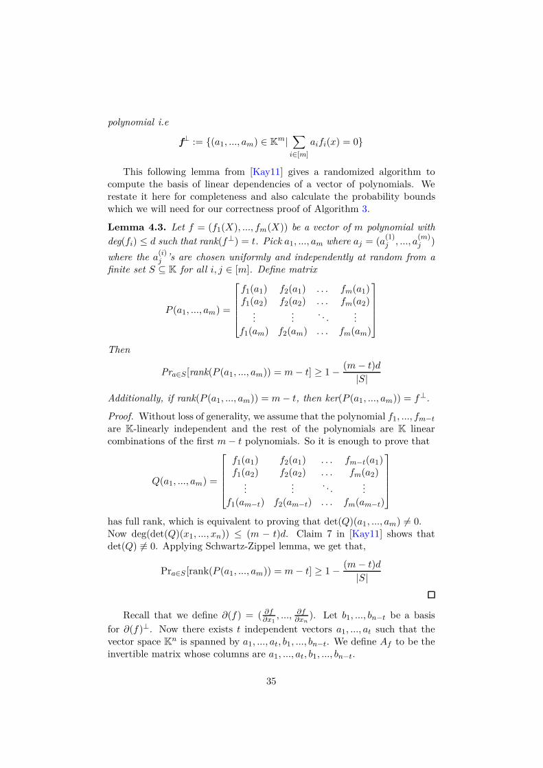
polynomial i.e

f⊥ := {(a1, ..., am) ∈ Km|∑

i∈[m]

aifi(x) = 0}

This following lemma from [Kay11] gives a randomized algorithm tocompute the basis of linear dependencies of a vector of polynomials. Werestate it here for completeness and also calculate the probability boundswhich we will need for our correctness proof of Algorithm 3.

Lemma 4.3. Let f = (f1(X), ..., fm(X)) be a vector of m polynomial with

deg(fi) ≤ d such that rank(f⊥) = t. Pick a1, ..., am where aj = (a(1)j , ..., a

(m)j )

where the a(i)j ’s are chosen uniformly and independently at random from a

finite set S ⊆ K for all i, j ∈ [m]. Define matrix

P (a1, ..., am) =

f1(a1) f2(a1) . . . fm(a1)f1(a2) f2(a2) . . . fm(a2)

......

. . ....

f1(am) f2(am) . . . fm(am)

Then

Pra∈S [rank(P (a1, ..., am)) = m − t] ≥ 1 − (m − t)d

|S|

Additionally, if rank(P (a1, ..., am)) = m − t, then ker(P (a1, ..., am)) = f⊥.

Proof. Without loss of generality, we assume that the polynomial f1, ..., fm−t

are K-linearly independent and the rest of the polynomials are K linearcombinations of the first m − t polynomials. So it is enough to prove that

Q(a1, ..., am) =

f1(a1) f2(a1) . . . fm−t(a1)f1(a2) f2(a2) . . . fm(a2)

......

. . ....

f1(am−t) f2(am−t) . . . fm(am−t)

has full rank, which is equivalent to proving that det(Q)(a1, ..., am) 6= 0.Now deg(det(Q)(x1, ..., xn)) ≤ (m − t)d. Claim 7 in [Kay11] shows thatdet(Q) 6≡ 0. Applying Schwartz-Zippel lemma, we get that,

Pra∈S [rank(P (a1, ..., am)) = m − t] ≥ 1 − (m − t)d

|S|

Recall that we define ∂(f) = ( ∂f∂x1

, ..., ∂f∂xn

). Let b1, ..., bn−t be a basis

for ∂(f)⊥. Now there exists t independent vectors a1, ..., at such that thevector space Kn is spanned by a1, ..., at, b1, ..., bn−t. We define Af to be theinvertible matrix whose columns are a1, ..., at, b1, ..., bn−t.

35

Theorem 4.4. [Car06b] The number of redundant variables in a polynomialf(x) equals the dimension of ∂(f)⊥. Furthermore, given a basis of ∂(f)⊥ ,the polynomial f(Af X) depends on only the first (n−dim(∂(f)⊥))) variables.

Lemma 4.5. If f can be written as a sum of r powers of linearly independentlinear forms, then the number of essential variables of f is equal to r.

Proof. Follows from Example 42 in [KS20].

We combine all the results in this section along with Theorem 3.1 to givea correctness proof for Algorithm 3.

Theorem 4.6. If an input P ∈ K[x1, ..., xn]d can not be written as∑t

i=1 αildi ,

where li are linearly independent linear forms and αi 6= 0 for all i ∈ [t], forany t ≤ n, then P is rejected by Algorithm 3 with high probability overthe choice of the random matrix R and the points α1, ..., αn. More for-mally, if the entries αi

j and ri,j are chosen uniformly and independently atrandom from a finite set S, then the input will be rejected with probability≥ (1 − 2(d−2)

|S| )(1 − n(d−1)|S| ).

Conversely, if P ∈ K[x1, ..., xn]d can be written as∑t

i=1 αildi where li are

linearly independent linear forms and αi 6= 0 for all i ∈ [t], then P will beaccepted by Algorithm 3 with high probability over the choice of the random

matrix R and the points a1, ..., an. More formally, if the entries α(i)j and ri,j

are chosen uniformly and independently at random from a finite set S, thenthe input will be accepted with probability ≥ (1 − t(d−1)

|S| )2 .

Proof. Let us assume that P has t essential variables and we fix M as givenby the algorithm. Then using Lemma 4.3 for fi = ∂P

∂xiand ai = αi, we get

that

Prα[v1, ..., vn−t is a basis for ∂(P )⊥] ≥ 1 − t(d − 1)

|S| .

The linear transformation A defined in the algorithm, satisfies the conditionsof the linear transformation defined in Theorem 4.4 with bi = vi and ai = ui

with probability ≥ 1 − t(d−1)|S| . Now, we define f(x) = P (Ax). This gives us

that

Prα[f(x) depends only on the first t variables] ≥ 1 − t(d − 1)

|S|

≥ 1 − n(d − 1)

|S| .

Using Theorem 3.1, we get that if f can not be written as a sum of t-manysum of d-th powers of linear forms for any t ≤ n, then the algorithm rejectsthe polynomial with probability ≥ (1 − 2(d−2)

|S| )(1 − n(d−1)|S| ).

For the converse, if f can be written as a sum of t-many sum of d-thpowers of linear forms, using Lemma 4.5, then the polynomial has t essentialvariables. Then the algorithm accepts P with probability ≥ (1− t(d−1)

|S| )2.

36

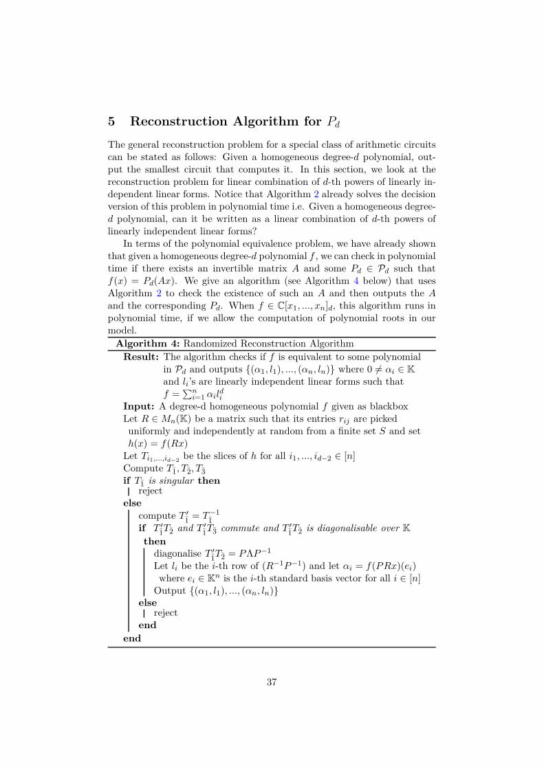
5 Reconstruction Algorithm for Pd

The general reconstruction problem for a special class of arithmetic circuitscan be stated as follows: Given a homogeneous degree-d polynomial, out-put the smallest circuit that computes it. In this section, we look at thereconstruction problem for linear combination of d-th powers of linearly in-dependent linear forms. Notice that Algorithm 2 already solves the decisionversion of this problem in polynomial time i.e. Given a homogeneous degree-d polynomial, can it be written as a linear combination of d-th powers oflinearly independent linear forms?

In terms of the polynomial equivalence problem, we have already shownthat given a homogeneous degree-d polynomial f , we can check in polynomialtime if there exists an invertible matrix A and some Pd ∈ Pd such thatf(x) = Pd(Ax). We give an algorithm (see Algorithm 4 below) that usesAlgorithm 2 to check the existence of such an A and then outputs the Aand the corresponding Pd. When f ∈ C[x1, ..., xn]d, this algorithm runs inpolynomial time, if we allow the computation of polynomial roots in ourmodel.

Algorithm 4: Randomized Reconstruction Algorithm

Result: The algorithm checks if f is equivalent to some polynomialin Pd and outputs {(α1, l1), ..., (αn, ln)} where 0 6= αi ∈ K

and li’s are linearly independent linear forms such thatf =

∑ni=1 αil

di

Input: A degree-d homogeneous polynomial f given as blackboxLet R ∈ Mn(K) be a matrix such that its entries rij are pickeduniformly and independently at random from a finite set S and seth(x) = f(Rx)

Let Ti1,...,id−2be the slices of h for all i1, ..., id−2 ∈ [n]

Compute T1, T2, T3

if T1 is singular thenreject

else

compute T ′1

= T −11


1T3 commute and T ′

1T2 is diagonalisable over K

then

diagonalise T ′1T2 = PΛP −1

Let li be the i-th row of (R−1P −1) and let αi = f(PRx)(ei)where ei ∈ Kn is the i-th standard basis vector for all i ∈ [n]

Output {(α1, l1), ..., (αn, ln)}else

rejectend

end

37

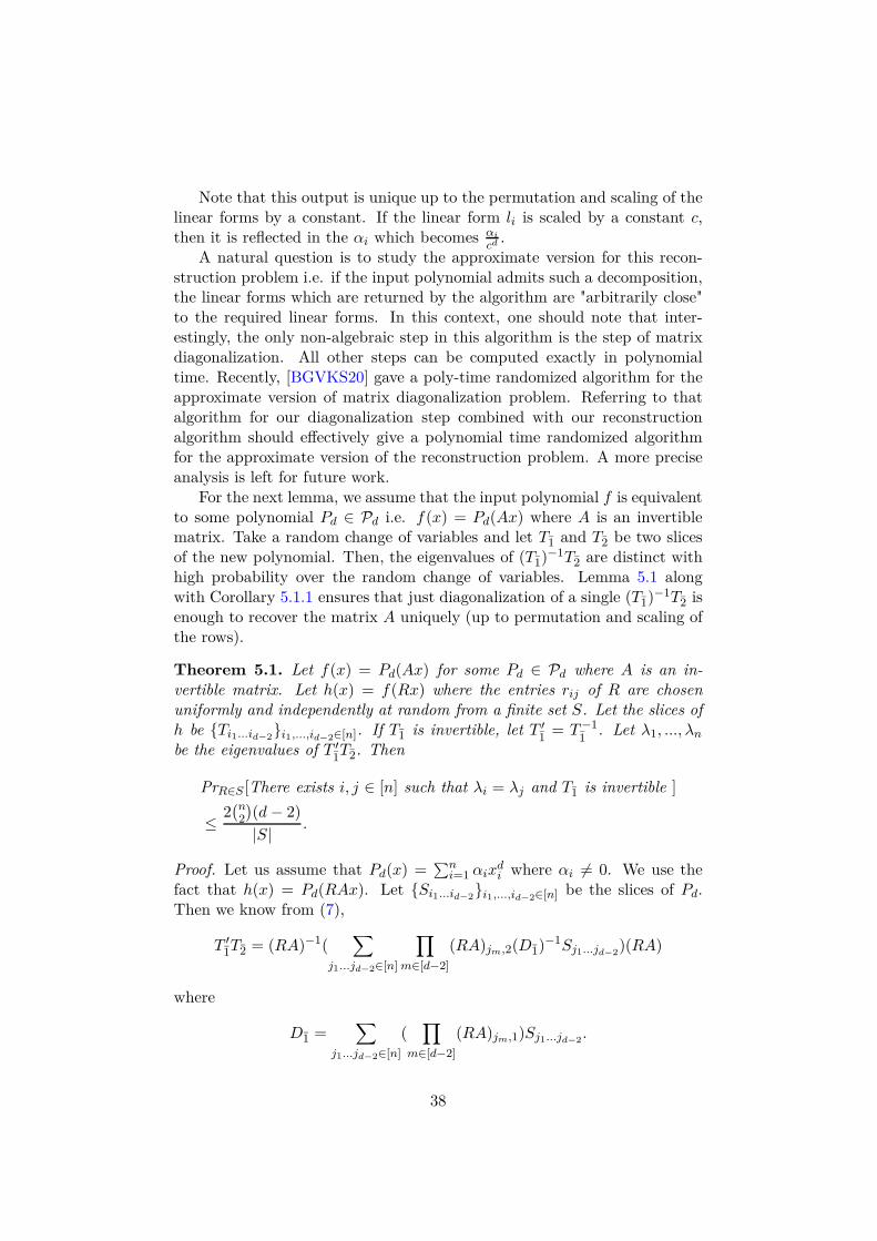
Note that this output is unique up to the permutation and scaling of thelinear forms by a constant. If the linear form li is scaled by a constant c,then it is reflected in the αi which becomes αi

cd .A natural question is to study the approximate version for this recon-

struction problem i.e. if the input polynomial admits such a decomposition,the linear forms which are returned by the algorithm are "arbitrarily close"to the required linear forms. In this context, one should note that inter-estingly, the only non-algebraic step in this algorithm is the step of matrixdiagonalization. All other steps can be computed exactly in polynomialtime. Recently, [BGVKS20] gave a poly-time randomized algorithm for theapproximate version of matrix diagonalization problem. Referring to thatalgorithm for our diagonalization step combined with our reconstructionalgorithm should effectively give a polynomial time randomized algorithmfor the approximate version of the reconstruction problem. A more preciseanalysis is left for future work.

For the next lemma, we assume that the input polynomial f is equivalentto some polynomial Pd ∈ Pd i.e. f(x) = Pd(Ax) where A is an invertiblematrix. Take a random change of variables and let T1 and T2 be two slicesof the new polynomial. Then, the eigenvalues of (T1)−1T2 are distinct withhigh probability over the random change of variables. Lemma 5.1 alongwith Corollary 5.1.1 ensures that just diagonalization of a single (T1)−1T2 isenough to recover the matrix A uniquely (up to permutation and scaling ofthe rows).

Theorem 5.1. Let f(x) = Pd(Ax) for some Pd ∈ Pd where A is an in-vertible matrix. Let h(x) = f(Rx) where the entries rij of R are chosenuniformly and independently at random from a finite set S. Let the slices ofh be {Ti1...id−2

}i1,...,id−2∈[n]. If T1 is invertible, let T ′1

= T −11

. Let λ1, ..., λn

be the eigenvalues of T ′1T2. Then

PrR∈S [There exists i, j ∈ [n] such that λi = λj and T1 is invertible ]

≤ 2(n

2

)

(d − 2)

|S| .

Proof. Let us assume that Pd(x) =∑n

i=1 αixdi where αi 6= 0. We use the

fact that h(x) = Pd(RAx). Let {Si1...id−2}i1,...,id−2∈[n] be the slices of Pd.

Then we know from (7),

T ′1T2 = (RA)−1(

∑

j1...jd−2∈[n]

∏

m∈[d−2]

(RA)jm,2(D1)−1Sj1...jd−2)(RA)

where

D1 =∑

j1...jd−2∈[n]

(∏

m∈[d−2]

(RA)jm,1)Sj1...jd−2.

38

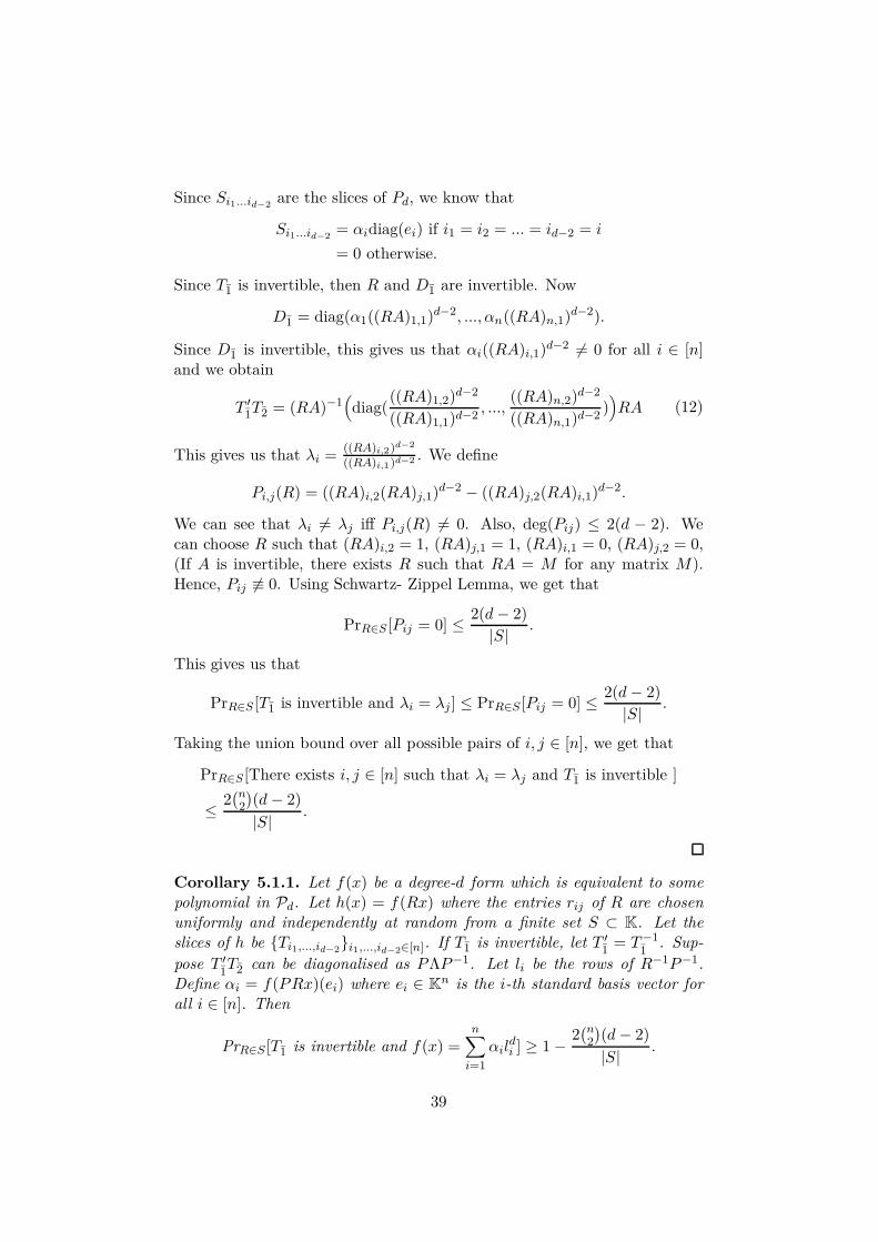
Since Si1...id−2are the slices of Pd, we know that

Si1...id−2= αidiag(ei) if i1 = i2 = ... = id−2 = i

= 0 otherwise.

Since T1 is invertible, then R and D1 are invertible. Now

D1 = diag(α1((RA)1,1)d−2, ..., αn((RA)n,1)d−2).

Since D1 is invertible, this gives us that αi((RA)i,1)d−2 6= 0 for all i ∈ [n]and we obtain

T ′1T2 = (RA)−1

(

diag(((RA)1,2)d−2

((RA)1,1)d−2, ...,

((RA)n,2)d−2

((RA)n,1)d−2))

RA (12)

This gives us that λi =((RA)i,2)d−2

((RA)i,1)d−2 . We define

Pi,j(R) = ((RA)i,2(RA)j,1)d−2 − ((RA)j,2(RA)i,1)d−2.

We can see that λi 6= λj iff Pi,j(R) 6= 0. Also, deg(Pij) ≤ 2(d − 2). Wecan choose R such that (RA)i,2 = 1, (RA)j,1 = 1, (RA)i,1 = 0, (RA)j,2 = 0,(If A is invertible, there exists R such that RA = M for any matrix M).Hence, Pij 6≡ 0. Using Schwartz- Zippel Lemma, we get that

PrR∈S [Pij = 0] ≤ 2(d − 2)

|S| .

This gives us that

PrR∈S [T1 is invertible and λi = λj ] ≤ PrR∈S [Pij = 0] ≤ 2(d − 2)

|S| .

Taking the union bound over all possible pairs of i, j ∈ [n], we get that

PrR∈S [There exists i, j ∈ [n] such that λi = λj and T1 is invertible ]

≤ 2(n

2

)

(d − 2)

|S| .

Corollary 5.1.1. Let f(x) be a degree-d form which is equivalent to somepolynomial in Pd. Let h(x) = f(Rx) where the entries rij of R are chosenuniformly and independently at random from a finite set S ⊂ K. Let theslices of h be {Ti1,...,id−2

}i1,...,id−2∈[n]. If T1 is invertible, let T ′1

= T −11

. Sup-

pose T ′1T2 can be diagonalised as PΛP −1. Let li be the rows of R−1P −1.

Define αi = f(PRx)(ei) where ei ∈ Kn is the i-th standard basis vector forall i ∈ [n]. Then

PrR∈S [T1 is invertible and f(x) =n

∑

i=1

αildi ] ≥ 1 − 2

(n2

)

(d − 2)

|S| .

39

Proof. By Theorem 5.1, we get that

PrR∈S [T1 is invertible and T ′1T2 has distinct eigenvalues]

≥ 1 − 2(n

2

)

(d − 2)

|S| .

We will now show that if T1 is invertible and T ′1T2 has distinct eigenvalues,

then f(x) =∑n

i=1 αildi .

If the eigenvalues are distinct, then the rank of the eigenspaces corre-sponding to each eigenvalue is 1. Hence, the eigenvectors of T ′

1T2 are unique

(up to a scaling factor). We already know that h(x) = Pd(Bx) for somePd ∈ Pd such that B is invertible. Then the columns of B−1 form the eigen-vectors of T ′

1T2. We take the diagonalization of T ′

1T2 into PΛP −1. Note

here that the columns of P form the eigenvectors for T ′1T2. The uniqueness

of eigenvectors of T ′1T2 gives us that the set of columns of P are essen-

tially the set of columns of B−1 upto a scaling factor. So this gives us thath(x) = P ′

d(P −1x) for some P ′d ∈ Pd. We know that f(x) = h(R−1x). This

gives us that f(x) = P ′d(R−1P −1)x. We define A = R−1P −1 and the i-th

row of A as li. This fixes the set of linear forms of the decomposition of theinput polynomial which are unique up to a scaling factor.Taking Pd = f(A−1x) gives the corresponding polynomial in Pd such thatf is equivalent to Pd. Now Pd =

∑ni=1 αix

di where αi 6= 0. Evaluating Pd at

ei ∈ Kn where ei is the i-th standard basis vector, returns the correspondingαi. Hence,

PrR∈S [f(x) =n

∑

i=1

αildi and T1 is invertible] ≥ 1 − 2

(n2

)

(d − 2)

|S| .

We combine all the results in this section along with Theorem 3.1 to givea correctness proof of Algorithm 4.

Theorem 5.2. If an input f ∈ K[x1, ..., xn]d is not equivalent to some poly-nomial in Pd, then f is rejected by Algorithm 4 with high probability. Moreformally, if the entries ri,j of R are chosen uniformly and independently atrandom from a finite set S, then the input will be rejected with probability≥ (1 − 2(d−2)

|S| ).

Conversely, if an input f ∈ K[x1, ..., xn]d is equivalent to some polynomial inPd, then Algorithm 4 outputs such a polynomial with high probability. Moreformally,if the entries of a matrix R are chosen uniformly and independentlyfrom a finite set S, then the algorithm outputs a set of linearly independentlinear forms li and corresponding coefficients αi 6= 0 such that f =

∑ni=1 αil

di

with probability ≥ 1 − (2(n

2)(d−2)

|S| + n(d−1)|S| ).

40

Proof. From Theorem 3.17, we get that if f is not equivalent to any polyno-mial in Pd, then f is rejected by Algorithm 4 with probability ≥ (1− 2(d−2)

|S| ).For the converse, we start by assuming that f is equivalent to some

polynomial in Pd. We know that if the first slice T1 of h(x) = f(Rx) is notinvertible, the Algorithm always makes an error and rejects the input. FromTheorem 3.8, we know that the subspace spanned by the slices of f is notweakly singular. We can therefore apply Lemma 3.9, we get that

PrR∈S [T1 is not invertible] ≤ n(d − 1)

|S| . (13)

Moreover if T1 is invertible, Lemma 3.10 shows that f will always beaccepted. Let the output of the algorithm be {(αi, li)}i∈[n]. So the only

possible error is when f 6= ∑

i∈[n] αildi . From Corollary 5.1.1, we get that

PrR∈S [Algorithm makes an error and T1 is invertible] ≤ 2(n

2

)

(d − 2)

|S| . (14)

Combining (13) and (14), we get that if f is equivalent to some polynomialin Pd, then Algorithm 4 returns a set of linearly independent linear forms liand corresponding coefficients αi 6= 0 (which are unique up to scaling and

permutation) such that f =∑n

i=1 αildi with probability ≥ 1 − (

2(n2)(d−2)

|S| +n(d−1)

|S| ).

We can also replace the call to Algorithm 2 in Algorithm 3 by a callto Algorithm 4 to similarly get a reconstruction algorithm for linear com-bination of powers of at most n linearly independent linear forms. Morespecifically, given a polynomial f in blackbox, it will check if there existsa decomposition of f =

∑ti=1 αil

di for some t ≤ n where li’s are linearly

independent and αi 6= 0 and outputs the decomposition, if it exists.

A Appendix: Complexity analysis for equivalence

to a sum of cubes

We first explain how the diagonalizability of a matrix can be tested efficientlywith an algebraic algorithm. This can be done thanks to the followingclassical result from linear algebra (see e.g. [HJ13], Corollary 3.3.8 for thecase K = C).

Lemma A.1. Let K be a field of characteristic 0 and let χM be the char-acteristic polynomial of a matrix M ∈ Mn(K). Let PM = χM

gcd(χM ,χ′

M) be

the square-free part of χM . The matrix M is diagonalisable over K iffPM (M) = 0. Moreover, in this case M is diagonalisable over K iff allthe roots of PM lie in K.

41

We prove the following lemma which shows that each entry of the slicesthat we need to compute can be computed using O(d) calls to the blackboxand O(d log3 d) many arithmetic operations. This proof is motivated fromthe idea of polynomial interpolation and the proof strategy of Lemma 4 in[FGS18].Their algorithm gives a poly(sd) runtime in our setting. In thissection, we will require this lemma only for d = 3, but we prove the generalform so that we can use it later in Appendix B.

Lemma A.2. Let f ∈ K[x1, ..., xn] be a homogeneous polynomial of degreed where |K| > d. If f is input as a blackbox C, then for some i ∈ [n]can compute the coefficient of xd−2

i xkxj using O(d) many oracle calls to theblackbox and O(M(d) log d) many arithmetic operations.

Proof. Here we use the standard trick of polynomial interpolation. With-out loss of generality, we assume that i = 1, that is we need to computecoeff

xd−21 xjxk

(f). So we can write,

C(x1, ..., xn) =d

∑

i=0

cixi1 where cj ∈ K[x2, ..., xn].

Now there are three cases:

• j = k = 1

• only one of j or k = 1

• j, k 6= 1.

Case 1: Evaluate the polynomial at the point (1, 0, ..., 0) ∈ Kn. This givesus the coefficient of xd

1 in f .Case 2: Exactly one of j or k is 1. Without loss of generality, we assumej = 1 and k = 2. So we want to compute coeff

xd−11 x2

(f). We evaluate the

polynomial f at the point t = (t, 1, 0, ..., 0) ∈ Kn. Now it’s easy to checkthat coefftd−1(f(t)) = coeff

xd−11 x2

(f). So we need to only interpolate and

calculate the coefficient of td−1 in f(t).Case 3: j, k 6= 1.

Now in this, there are two cases :

• j = k = 2 : Here we take a similar strategy as Case 2. We evaluatef at t = (t, 1, 0, ..., 0) ∈ Kn. Then coefftd−2(f(t)) = coeff

xd−21 x2

2(f) So

interpolate and compute the coefficient of td−2 in f(t).

• The final case is when the indices are all distinct. Let j = 2 andk = 3 without loss of generality. We evaluate the polynomial f att = (t, 1, 1, 0, ..., 0) ∈ Kn. Now

coefftd−2(f(t)) = coeffxd−2

1 x22(f) + coeff

xd−21 x2x3

(f) + coeffxd−2

1 x23(f)

42

Now, using the previous case, we compute coeffxd−2

1 x22(f) and coeff

xd−21 x2

3(f),

subtract them from coefftd−2(f(t)) and return the answer.

Each case of this algorithm requires us to do univariate polynomial inter-polation at most constantly many number of times and this can be donein time O(M(d) log d) [GG13] (Section 10.2) where M(d) is the number ofarithmetic operations for polynomial multiplication. Rest of the operationscan be done in time O(1). It also requires O(d) many oracle calls to theblackbox.So the algorithm uses O(M(d) log d) many arithmetic operations and O(d)many oracle calls to the blackbox.

Theorem A.3. If a degree 3 form f ∈ K[x1, ..., xn] is given in dense rep-resentation, Algorithm 1 runs in time O(nω+1) where ω is the exponent ofmatrix multiplication.If the degree 3 form f ∈ K[x1, ..., xn] is given as a blackbox then the algo-rithm makes O(n2) many calls to the blackbox and O(nω+1) many arithmeticoperations.

Proof. The following are the different stages of computation required in thisalgorithm:

1. Recall from Theorem 2.2, the slices Ti of h = f(Rx) are given bythe formula Tk = RT (

∑

i∈[n] ri,kSi)R. If the polynomial is input indense representation, then the elements of Si can be computed fromthe coefficients of f . Then we take linear combinations of the Si’s andcomputing T1, T2, T3 takes O(n3) many arithmetic operations.If the polynomial is given as a blackbox, we compute x′ = Rx and wecall the blackbox on this input.

2. Compute T1, T2, T3 We know

(Tk)ij =1

3!∂xixjxk

(h)

So we can extract each entry of Tk using constant many calls to theblackbox and constantly many arithmetic operations using Lemma A.2.There are in total 3n2 such entries that we need to compute. So thetotal number of calls to the blackbox is O(n2) and the number ofarithmetic operations is O(n2).

3. Check if T1 is invertible. If invertible, compute T ′1 = T −1

1 .This can be done in time at most O(n3). (Faster algorithms exist[GG13] but this bound is enough since it is not the most expensivestep of the algorithm.)

43

4. Checking commutativity of T ′1T2 and T ′

1T3.Here we compute the product T ′

1T2T ′1T3 and T ′

1T3T ′1T2 and check if

their difference is 0. This can be done in time O(nω).

5. Checking the diagonalisability of T ′1T2:

Here we use Lemma A.1. Hence there are four steps:

• Compute the characteristic polynomial of M i.e. χM . This canbe done in time O(nω log n). [KG85]

• Compute gcd(χM , χ′M , ). Since, deg(χM ) ≤ n, this can be done

in O(n2) using Euclidean Algorithm. [GG13]

• Compute PM = χM

gcd(χM ,χ′

M) . This is can be computed in O(n2)

using the standard long-division algorithm.

• Check if PM (M) = 0. Using Horner’s Method, we can evaluatethe polynomial at M using n many matrix multiplications only.Hence, computing PM (M) takes O(nω+1) time.

Hence, we can conclude that the diagonalisability of T ′1T2 can be

checked in time O(nω+1). Note that this is the most expensive step ofthe algorithm!

So we conclude that if the polynomial is given as an input in the dense rep-resentation model, then the algorithm runs in time O(nω+1).If the polynomial is given as a blackbox, then the algorithm makes O(n2)many oracle calls to the blackbox and takes O(nω+1) many arithmetic op-erations.

A.1 Computing the complexity of the randomized algorithmin [KS20] and comparing it with our algorithm :

Recall the [KS20] equivalence from Section 1.2. The algorithm proceeds asfollows:

1. Pick a random matrix R ∈ Mn(K) and set h(x) = f(Rx).

2. Let T1, ..., Tn be the slices of h. If T1 is singular, reject. Otherwise,compute T ′

1 = T −11 .

3. If the matrices T ′1Tk commute and are all diagonalisable over K, accept.

Otherwise, reject.

The following are the different stages of computation required in this algo-rithm:

1. If the polynomial is input in dense representation, here we have tocompute all the slices T1, ..., Tn and following the proof of Theorem A.3,

44

this takes O(n4) many arithmetic operationsIf the polynomial is given as a blackbox, we compute x′ = Rx. Andwe call the blackbox on this input.

2. Compute T1, T2, ..., Tn We know

(Tk)ij =1

3!∂xixjxk

(h).

So we can extract each entry of Tk using constant many calls to theblackbox and constantly many arithemtic operations using Lemma A.2.There are in total n3 such entries that we need to compute. So thetotal number of calls to the blackbox is O(n3) and the number ofarithmetic operations is O(n3)

3. Check if T1 is invertible. If invertible, compute T ′1 = T −1

1 .This can be done in time at most O(n3).

4. Checking pairwise commutativity of {T ′1Tj}j∈[n]

Here we compute the product T ′1TiT

′1Tj and T ′

1TjT′1Ti and check if

their difference is 0. For each pair, this can be done in time O(nω).Since there are

(n2

)

many pairs, this can be done in time O(nω+2).

5. Checking the diagonalisability of T ′1Tj for all j ∈ [n]:

As we showed that the diagonalisability of each T ′1Tj can be checked in

time O(nω+1). So the total time taken for checking diagonalisabilityof n such matrices is O(nω+2).

So we conclude that if the polynomial is given as an input in the dense rep-resentation model, then the algorithm runs in time O(nω+2).If the polynomial is given as a blackbox, then the algorithm makes O(n3)many calls to the blackbox and requires O(nω+2) many arithmetic opera-tions.

So we manage to shave a factor of n from [KS20] in both cases: whenthe polynomial is given in dense representation as well as when it is inputas an arithmetic circuit.

B Complexity analysis for equivalence to some poly-

nomial in Pd

B.1 Complexity Analysis in the algebraic model

In this section, we provide a detailed complexity analysis of Algorithm 2.We show that if a degree d polynomial in n variables over C is given as ablackbox, the algorithm makes poly(n, d) many calls to the blackbox andperforms poly(n, d) many arithmetic operations to decide if f is equivalentto some polynomial in Pd.

45

Theorem B.1. If a degree-d form f ∈ C[x1, ..., xn] is given as a blackbox,then Algorithm 2 makes O(n2d) many calls to the blackbox and requiresO(n2d log2 d log log d + nω+1) many arithmetic operations.

Proof. The following are the different stages of computation required in thisalgorithm:

1. If the polynomial is given as a blackbox, we compute x′ = Rx. Andwe call the blackbox on this input.

2. Compute T1, T2, T3. We know that (Tk)ij = 1d!∂xixjxd−2

k

(h).So we

can extract each entry of Ti using O(d) many oracle calls to C ′ andO(M(d) log d) many arithmetic operations using Lemma (A.2). Thereare in total 3n2 such entries that we need to compute. So this entireoperation can be done using O(n2d) many oracle calls to the blackboxand O(n2M(d) log d) many arithmetic operations.

3. Check if T1 is invertible. If invertible, compute T ′1

= (T1)−1

4. Checking commutativity of T ′1T2 and T ′

1T3.

5. Checking the diagonalisability of T ′1T2:

Steps (3), (4) and (5) are exactly the same as Theorem A.3. This is becausethey don’t require any assumptions on T1, T2, T3 except for the fact thatthey are n × n matrices. Thus, from the proof of Theorem A.3, we get thatthese steps can be checked in O(nω+1) many arithmetic operations.

So we conclude that if the polynomial is given as a blackbox, then thealgorithm makes O(n2d) many calls to the blackbox; the number of arith-metic operations required is O(n2M(d) log d + nω+1).Since M(d) = O(d log d log log d), the number of arithmetic operations isO(n2d log2 d log log d + nω+1).

B.2 Complexity analysis for the bit model

We look at the case where f ∈ Q[x1, ..., xn] is a degree-d form and we wantto check if it can be written as a linear combination of dth powers of linearforms over R or C. Our algebraic algorithms run in polynomial time inthe standard bit model of computation, i.e., they are “strongly polynomial”algorithms (this is not automatic due to the issue of coefficient growth duringthe computation). For a detailed discussion of how the previous algorithmsfail to give a polynomial time algorithm for this problem in this model, referto Section 1.1 from [KS20].

We try to estimate the complexity of each step of the algorithm in thestandard bit model of computation, following the proof of Theorem B.1.In Step (1), we take a matrix R such that its entries ri,j are picked uni-formly and independently at random from a finite set S.Hence the bit

46

size of the entries of R are bounded by log(|S|) + 1. We define h =f(Rx). Recall from Theorem 3.2, that the slices Ti of h can be written asRT (

∑

i1,...,id−2∈[n](∏

m∈[d] rim,i)Si1...id−2)R. The entries of the slices Si1...id−2

are essentially the coefficients of f . So they are bounded by the bit size ofthe maximum coefficient in f which we define to be bf . Therefore, the bitsize of each element of Ti is b := poly(log(|S|), log(n), d, bf ) for all i. Now theelements of T1, T2, T3 are computed using Lemma A.2 that uses polynomialinterpolation and hence, computing these matrices takes time poly(n, d, b).In Step (3), we check if the slice T1 is invertible and if invertible, it is in-verted. Since the bit-size of the inputs of T1 are bounded by b, the matrixcan be inverted using Bareiss’ Algorithm [Bar68] in time poly(n, d, b). InStep (4), testing commutativity of T ′

1T2 and T ′

1T3 requires only matrix mul-

tiplication which does not blow up the entry of the matrices and hence, thisstep can be done in time poly(n, d, b). In Step (5), we need to check the di-agonalisability of M = T ′

1T2. Over the field of complex numbers it therefore

suffices to check that PM (M) = 0 which can be done in time poly(n, d, b).For the discussion of how the same can be executed over R, refer to Section4 of [KS20].

So the total time required for the entire computation in the bit model ofcomplexity is poly(n, d, log(|S|), bf ) where bf is the bit size of the maximumcoefficient in f and S is the set from which the entries of R are pickeduniformly and independently at random.

C Complexity analysis for variable minimization

In this section, we provide a detailed complexity analysis of Algorithm 3.We show that if a degree d polynomial in n variables over C is given as ablackbox, the algorithm performs poly(n, d) many calls to the blackbox andperforms poly(n, d) many arithmetic operations to check if the polynomialcan be written as a linear combination of t many linearly independent linearforms for some t ≤ n (see Theorem C.2).

In the next lemma, we show that given a blackbox computing the polyno-mial, we can compute the partial derivative with respect to a single variableat a given point in O(d) many oracle calls and poly(d) arithmetic operations.

Lemma C.1. Given a blackbox computing P ∈ K[x1, ..., xn] of degree atmost d, and given points α1, ..., αn ∈ Kn, we can compute the matrix Msuch that Mij = ∂xi

(P )(αj) using O(n2d) many oracle calls to the blackboxand O(n2M(d) log d) many arithmetic operations.

Proof. We assume i = 1. Given points a1, ..., an ∈ K, ∂x1(P )(a1, ..., an) canbe computed using the following steps of computation:

• Compute the polynomial P (x, a2, ..., an) explicitly using polynomialinterpolation. This can be done using O(M(d) log d) many arithmetic

47

operations and d+1 many calls to the blackbox. [GG13] (Section 10.2)

• Compute ∂x(P (x, a2, ..., an)) using O(d) many arithmetic operations.

• evaluate it at x = a1, which requires O(d) many arithmetic operations.

We do this for every (a1, ..., an) = (α(1)j , ..., α

(n)j ) for all j ∈ [n]. Thus

each row of the matrix M can be computed using O(nM(d) log d) manyoperations. For each xi such that i ∈ [n], a similar algorithm works and thematrix M can be computed using O(n2M(d) log d) arithmetic operationsand O(n2d) many calls to the blackbox.

Now we are in a position to analyse the complexity of Algorithm 3

Theorem C.2. Given a blackbox computing a polynomial P ∈ K[x1, ..., xn]dwith t essential variables, the algorithm makes O(n2d) many calls to theblackbox and requires O(nω + n2M(d) log d + tω+1) many arithmetic opera-tions.

Proof. The following are the steps of the algorithm:

• Using Lemma C.1, we know that the matrix M can be computed intime O(n2M(d) log d) many arithmetic operations and O(n2d) manycalls to the blackbox.

• The basis of ker(M) can be computed and the basis can be completedusing O(nω) many arithmetic operations.

• For n = t, using Theorem B.1 the algorithm checks equivalence usingO(t2d) many calls to the blackbox and O(t2M(d) log d + tω+1) manyarithmetic operations.

So we conclude that if the polynomial is given as a blackbox, then thealgorithm makes O(n2d) many calls to the blackbox and the number ofarithmetic operations required is O(nω + n2M(d) log d + tω+1).

Using Section B.2 and the fact that we just need to do polynomial inter-polation and completion of the basis, we conclude that Algorithm 3 takestime poly(n, d, log(|S|), bf ) in the bit model of computation. Here bf is thebit size of the maximum coefficient in f and S is the set from which the

entries of R and α(i)j s are picked uniformly and independently at random.

Acknowledgements

We would like to thank Mateusz Skomra for useful discussions in the earlystages of this work, and Frédéric Magniez for discussions on commutativitytesting.

48

References

[AGH+14] Animashree Anandkumar, Rong Ge, Daniel Hsu, Sham M.Kakade, and Matus Telgarsky. Tensor decompositions for learn-ing latent variable models. Journal of Machine Learning Re-search, 15(80):2773–2832, 2014.

[Bar68] Erwin H. Bareiss. Sylvester’s identity and multistep integer-preserving gaussian elimination. Mathematics of Computation,22(103):565–578, 1968.

[BCMT10] Jérôme Brachat, Pierre Comon, Bernard Mourrain, and EliasTsigaridas. Symmetric tensor decomposition. Linear Algebraand its Applications, 433(11-12):1851–1872, 2010.

[BCSS98] L. Blum, F. Cucker, M. Shub, and S. Smale. Complexity andReal Computation. Springer-Verlag, 1998.

[BGI11] Alessandra Bernardi, Alessandro Gimigliano, and Monica Ida.Computing symmetric rank for symmetric tensors. Journal ofSymbolic Computation, 46(1):34–53, 2011.

[BGVKS20] Jess Banks, Jorge Garza-Vargas, Archit Kulkarni, and NikhilSrivastava. Pseudospectral shattering, the sign function, anddiagonalization in nearly matrix multiplication time. In 2020IEEE 61st Annual Symposium on Foundations of ComputerScience (FOCS), pages 529–540, 2020.

[BSS89] L. Blum, M. Shub, and S. Smale. On a theory of computationand complexity over the real numbers: NP-completeness, recur-sive functions and universal machines. Bulletin of the AmericanMathematical Society, 21(1):1–46, July 1989.

[BSV21] Vishwas Bhargava, Shubhangi Saraf, and Ilya Volkovich. Re-construction algorithms for low-rank tensors and depth-3 mul-tilinear circuits. arXiv preprint arXiv:2105.01751, 2021.

[Car06a] Enrico Carlini. Reducing the number of variables of a poly-nomial. In Algebraic geometry and geometric modeling, Math.Vis., pages 237–247. Springer, Berlin, 2006.

[Car06b] Enrico Carlini. Reducing the number of variables of a poly-nomial. In Mohamed Elkadi, Bernard Mourrain, and RagniPiene, editors, Algebraic Geometry and Geometric Modeling,pages 237–247, Berlin, Heidelberg, 2006. Springer Berlin Hei-delberg.

49

[CG05] Guillaume Cheze and André Galligo. Four lectures on polyno-mial absolute factorization. In Solving polynomial equations,pages 339–392. Springer, 2005.

[CL07] Guillaume Chèze and Grégoire Lecerf. Lifting and recombina-tion techniques for absolute factorization. Journal of Complex-ity, 23(3):380–420, 2007.

[DL78] Richard A. Demillo and Richard J. Lipton. A probabilisticremark on algebraic program testing. Information ProcessingLetters, 7(4):193–195, 1978.

[FGS18] Michael A. Forbes, Sumanta Ghosh, and Nitin Saxena. To-wards Blackbox Identity Testing of Log-Variate Circuits. In45th International Colloquium on Automata, Languages, andProgramming (ICALP 2018), 2018.

[Fre79] Rusin, š Freivalds. Fast probabilistic algorithms. In Interna-tional Symposium on Mathematical Foundations of ComputerScience (MFCS), pages 57–69. Springer, 1979.

[Gao03] Shuhong Gao. Factoring multivariate polynomials via par-tial differential equations. Mathematics of computation,72(242):801–822, 2003.

[GG13] Joachim von zur Gathen and Jürgen Gerhard. Modern Com-puter Algebra. Cambridge University Press, USA, 3rd edition,2013.

[GGKS19] Ankit Garg, Nikhil Gupta, Neeraj Kayal, and Chandan Saha.Determinant equivalence test over finite fields and over Q. InElectronic Colloquium on Computational Complexity (ECCC),volume 26, page 42, 2019.

[GMKP17] Ignacio García-Marco, Pascal Koiran, and Timothée Pecatte.Reconstruction algorithms for sums of affine powers. In Proc.International Symposium on Symbolic and Algebraic Computa-tion (ISSAC), pages 317–324, 2017.

[GMKP18] Ignacio García-Marco, Pascal Koiran, and Timothée Pecatte.Polynomial equivalence problems for sums of affine powers.In Proc. International Symposium on Symbolic and AlgebraicComputation (ISSAC), 2018.

[Har70] R. Harshman. Foundations of the parafac procedure: Modelsand conditions for an "explanatory" multi-model factor analy-sis. 1970.

50

[HJ13] Roger Horn and Charles Johnson. Matrix Analysis. CambridgeUniversity Press (second edition), 2013.

[Kay11] Neeraj Kayal. Efficient algorithms for some special cases ofthe polynomial equivalence problem. In Symposium on Dis-crete Algorithms (SODA). Society for Industrial and AppliedMathematics, January 2011.

[KB09] T. Kolda and B. Bader. Tensor decompositions and applica-tions. SIAM Rev., 51:455–500, 2009.

[KG85] Walter Keller-Gehrig. Fast algorithms for the characteristicspolynomial. Theoretical Computer Science, 36:309 – 317, 1985.

[KNST18] Neeraj Kayal, Vineet Nair, Chandan Saha, and Sébastien Tave-nas. Reconstruction of full rank algebraic branching programs.ACM Transactions on Computation Theory (TOCT), 11(1):2,2018.

[KS09] Zohar Karnin and Amir Shpilka. Reconstruction of general-ized depth-3 arithmetic circuits with bounded top fan-in. In24th Annual IEEE Conference on Computational Complexity(CCC), pages 274–285, 2009.

[KS19] Neeraj Kayal and Chandan Saha. Reconstruction of non-degenerate homogeneous depth three circuits. In Proc. 51stAnnual ACM Symposium on Theory of Computing (STOC),pages 413–424, 2019.

[KS20] Pascal Koiran and Mateusz Skomra. Derandomization and ab-solute reconstruction for sums of powers of linear forms. arXivpreprint arXiv:1912.02021, 2020. To appear in TheoreticalComputer Science, 2021.

[MN07] Frédéric Magniez and Ashwin Nayak. Quantum complexityof testing group commutativity. Algorithmica, 48(3):221–232,2007.

[Moi18] A. Moitra. Algorithmic Aspects of Machine Learning. Cam-bridge University Press, 2018.

[Pak12] Igor Pak. Testing commutativity of a group and the power ofrandomization. LMS Journal of Computation and Mathemat-ics, 15:38–43, 2012.

[RS00] Sridhar Rajagopalan and Leonard J Schulman. Verificationof identities. SIAM Journal on Computing, 29(4):1155–1163,2000.

51

[Sch80] J. T. Schwartz. Fast probabilistic algorithms for verification ofpolynomial identities. J. ACM, 27(4):701–717, October 1980.

[Sha09] Hani Shaker. Topology and factorization of polynomials. Math-ematica Scandinavica, pages 51–59, 2009.

[Shi16] Yaroslav Shitov. How hard is the tensor rank? arXiv preprintarXiv:1611.01559, 2016.

[Shp09] Amir Shpilka. Interpolation of depth-3 arithmetic circuitswith two multiplication gates. SIAM Journal on Computing,38(6):2130–2161, 2009.

[SS71] A. Schönhage and V. Strassen. Schnelle multiplikation großerzahlen. Computing, 7(3):281–292, Sep 1971.

[Zip79] Richard Zippel. Probabilistic algorithms for sparse polynomi-als. In Symbolic and Algebraic Computation, pages 216–226,Berlin, Heidelberg, 1979. Springer Berlin Heidelberg.

52

Black Box Absolute Reconstruction for Sums of Powers ... - arXiv

Documents

Transcript of Black Box Absolute Reconstruction for Sums of Powers ... - arXiv