Absolute Identification by Relative Judgment

Absolute Identification 1

Running Head: RELATIVE JUDGMENT MODEL

Absolute Identification by Relative Judgment

Neil Stewart, Gordon D. A. Brown, and Nick Chater

University of Warwick, England

Stewart, N., Brown, G. D. A., & Chater, N. (2005). Absolute identification by relative

judgment. Psychological Review, 112, 881-911.


Abstract

In unidimensional absolute identification tasks, participants identify stimuli that vary along a

single dimension. Performance is surprisingly poor compared to discrimination of the same

stimuli. Existing models assume that identification is achieved using long-term representations

of absolute magnitudes. We propose an alternative relative judgment model (RJM) in which

the elemental perceptual units are representations of the differences between current and

previous stimuli. These differences are used, together with the previous feedback, to respond.

Without using long-term representations of absolute magnitudes, the RJM accounts for (a)

information transmission limits, (b) bowed serial position effects, and (c) sequential effects,

where responses are biased towards immediately preceding stimuli but away from more distant

stimuli (assimilation and contrast).


Absolute Identification by Relative Judgment

Miller (1956) drew attention to a curious phenomenon. People have great difficulty

identifying stimuli from a set that varies along a single psychological continuum, even though

their ability to discriminate pairs of stimuli from the set suggests that they should be very good

at the identification task. This phenomenon can be seen across a wide range of stimulus

attributes - the frequency and loudness of tones, the strength of tastes and smells, the

magnitude of lengths and areas, the hue and brightness of colors, and the intensity and

numerousness of cutaneous stimulation - suggesting some common and fundamental source of

the limitation.

In an absolute identification task, participants are required to identify, with a unique

label, stimuli drawn from a set of items that vary along only a single continuum. Typically,

stimuli are evenly psychologically spaced. A stimulus's label is normally its ordinal position

within the set. Three key phenomena, which we review in more detail below, are observed.

First, there is a severe limit in the information transmitted from stimulus to response (i.e., the

size of the set for which members can be identified perfectly) even when adjacent stimuli are

perfectly discriminable. Second, a bow effect is observed when identification accuracy is

plotted against stimulus, with an advantage for the smallest and largest stimuli. Third, there are

strong sequential effects, whereby the stimuli on previous trials exert a strong bias on the

response to the current stimulus.

Many theoretical accounts have been offered of one or more of these phenomena.

Nearly all of these models have in common the assumption that in an absolute identification

task a representation of the absolute magnitude of the current stimulus is compared to some

long-term representations of the absolute magnitudes either of other stimuli from the set,

particular anchor values, or particular criterial values. However, in a review for the centenary

issue of Psychological Review, Shiffrin and Nosofsky (1994, p. 359) conclude that since

Miller's (1956) classic article "...a fully unified account of the numerous range, edge, and


sequential effects has not been achieved."

Here, in contrast to existing models (excepting Laming, 1984), we offer a relative

judgment model (RJM) of absolute identification. The RJM does not utilize long-term

representations of absolute magnitudes. Instead, the difference between the current stimulus

and the previous stimulus is used, in conjunction with the feedback from the previous trial, to

generate a response. Thus, the magnitude of the current stimulus is judged relative to the

magnitude of only the immediately preceding stimulus (hence the name RJM). In this article,

we review existing models of absolute identification and show that none offers a complete

account of the phenomena described above. We then show that the RJM offers a unified

account of these phenomena, and present new experimental evidence that supports the model.

We begin with a review of the key empirical results.

Empirical Results in Absolute Identification

Information Transmission Limit

Using multivariate information transmission as a dependent variable (McGill, 1954), it

is possible to measure the information transmitted1 in an absolute identification task. If

performance in an absolute identification task were perfect, the information transmitted would

grow as the number of stimuli is increased. For example, perfect identification of two equally

probable stimuli carries 1 bit of information, identification of four stimuli carries 2 bits, of

eight stimuli carries 3 bits, and so on. However, the information transmitted from stimulus to

response (sometimes, channel capacity) in an absolute identification task seems to be limited to

very few bits (see Table 1) corresponding to perfect identification of very few stimuli across a

very wide range of stimulus attributes (see Garner, 1962; Laming, 1984; Miller, 1956 for

reviews). Figure 1 shows information transmitted as a function of the number of stimuli in the

set (with range of the stimuli held constant) for data from Garner (1953) and Pollack (1952).

(In all figures that present data, data are collapsed across participants.) With a small number of

stimuli, obviously less information must be transmitted, but as the number of stimuli increases,


the information transmitted from stimulus to response does not continue to increase. Although

an increase in the range of stimuli (number held constant), and hence the separation of the

stimuli, will produce an initial increase in information transmitted, the increase is a negatively

accelerated function of range, and quickly reaches an asymptote once adjacent stimuli are

discriminable (Alluisi & Sidorsky, 1958; Braida & Durlach, 1972; Eriksen & Hake, 1955a;

Pollack, 1952).

Bow or Edge Effects in the Serial Position Curve

When accuracy is plotted as a function of the rank of the stimulus within the stimulus

set, a characteristic bow is observed in the resulting serial position curve (e.g., Kent &

Lamberts, in press; Lacouture & Marley, 2004; Murdock, 1960; W. Siegel, 1972).

Performance on stimuli at the ends of the range is better than performance on mid-range

stimuli even though, when presented in isolation, any two adjacent stimuli may be perfectly

discriminable. As for information transmission, once stimuli are pairwise perfectly

discriminable, increased spacing of items leads, at best, to only slight improvements in

accuracy (Braida & Durlach, 1972; Brown, Neath, & Chater, 2002; Gravetter & Lockhead,

1973; Hartman, 1954; Lacouture, 1997; Luce, Green, & Weber, 1976; Pollack, 1952). Figure

2 shows the very similar stimulus-response confusion matrices obtained by Brown et al.

(2002) for absolute identification of tones varying in their frequency. Tones were

geometrically spaced, with each tone a constant ratio higher in frequency than the immediately

lower tone. (Following Weber's Law, geometric spacing is typically used to produce stimuli

that are presumed to be equally psychologically spaced.) Each confusion matrix is for a

different stimulus spacing (from 420 - 563 Hz in the narrow spacing condition to 363 - 652 Hz

in the wide spacing condition). As Figure 2 shows, increasing the stimulus spacing had almost

no effect on performance.

Increasing the number of stimuli in an absolute identification task increases the size of

the bow effect (Alluisi & Sidorsky, 1958; Durlach & Braida, 1969; Lacouture & Marley,


1995; Pollack, 1953; W. Siegel, 1972; Weber, Green, & Luce, 1977). Figure 3 shows the

serial position curves obtained by Lacouture and Marley (1995; see also Kent & Lamberts, in

press; Lacouture, Li, & Marley, 1998) for different stimulus set sizes, with a larger bow effect

for larger set sizes. Note that although Stimuli 5 and 6 can be nearly perfectly discriminated

when they constitute the entire stimulus set, performance on these same stimuli drops

considerably when they are identified within a larger stimulus set. Simply shifting all the stimuli

along the dimension, so that each stimulus increased in value by a constant multiplicative

factor, has no effect on the accuracy against stimulus magnitude curve (Lacouture, 1997). The

bow effect remains even after extensive practice, although small improvements in accuracy are

observed (Alluisi & Sidorsky, 1958; Hartman, 1954; Weber et al., 1977; but see Rouder,

Morey, Cowan, & Pfaltz, 2004, for a larger practice effect). The bow effect is greatly reduced

by correcting for the asymmetry of errors on extreme verses interior stimuli (Weber et al.,

1977), suggesting that the restricted opportunity to make errors at the ends of the range is a

major factor underlying the bow effect (see also Eriksen & Hake, 1957). The bow effect is not

due to response bias (at least, not response bias alone). In data where end responses are not

used more frequently than central responses, the effect is still observed (W. Siegel, 1972). In

our data from Experiment 1, the bow is observed although there is a bias against responding

with extreme categories.

Sequential Effects

We know of no absolute identification experiment where strong sequence effects

(where the response to the current stimulus is shown to depend on previous stimuli and

responses) are not found. Of course, when performance in an absolute identification task is

perfect, then there are no sequential dependencies. Thus the existence of sequential

dependencies is likely to provide a useful insight into processing in an absolute identification

task.

The most salient sequential effect is that the response given to the current stimulus is


shown to be assimilated to the immediately preceding stimulus (Garner, 1953; Holland &

Lockhead, 1968; Hu, 1997; Lacouture, 1997; Lockhead, 1984; Long, 1937; Luce, Nosofsky,

Green, & Smith, 1982; Petrov & Anderson, in press; Purks, Callahan, Braida, & Durlach,

1980; Rouder et al., 2004; Staddon, King, & Lockhead, 1980; Stewart, 2001; Ward &

Lockhead, 1970, 1971). In other words, participants are systematically biased to respond as if

the current stimulus is nearer to the previous stimulus than it actually is. Figure 4 shows data

from the feedback condition of Ward and Lockhead's (1970) absolute identification

experiment. Stimuli were tones varying in loudness. The average error in responding on the

current trial is plotted for each stimulus as a function of the stimulus on the previous trial.

When the current stimulus is greater than the previous stimulus, the error is negative (i.e., the

stimulus is underestimated); when the current stimulus is less than the previous stimulus, the

error is positive. The five lines are approximately parallel, with positive slopes, demonstrating

that assimilation takes place for all combinations of current and previous stimuli (Lockhead,

1984). Assimilation to preceding items is also observed in magnitude estimation tasks (e.g.,

Jesteadt, Luce, & Green, 1977), in matching tasks (Stevens, 1975, p. 275), and in relative

intensity judgment tasks (Lockhead & King, 1983).

The effect of stimuli further back in the sequence on the current response is the

opposite, that is, there is a contrast effect (Holland & Lockhead, 1968; Lacouture, 1997;

Ward & Lockhead, 1970, 1971). Assimilation to the previous trial and contrast to trials

further back has been demonstrated within the same experiments, for the same participants.

Figure 5 shows the average error on the current trial (averaged across all possible stimuli on

the current trial) as a function of the stimulus k trials ago for data from Holland and Lockhead

(1968), Lacouture (1997), and Ward and Lockhead (1970). As described above, assimilation

is shown to the stimulus on the immediately preceding trial (k = 1). Stimuli on less recent trials

(k > 1) exhibit contrast, as shown by the reversal in the sign of the error. The contrast effect is

smaller than the assimilation, and the error dependency reduces to zero with increased


numbers of intervening trials.

In the experiments on sequence effects discussed so far stimulus, response and

feedback are all highly correlated. Which of these is the basis for assimilation (and contrast)?

We focus on this question for the remainder of this section.

The sequence effects observed are dependent on the quality of stimulus presentation.

Ward and Lockhead (1971) examined performance in a standard absolute identification

experiment using line length. When task difficulty was increased, by reducing the luminance

and duration of line length presentations, more assimilation was observed. In the difficult

condition, accuracy was low and therefore the correlation between stimuli and responses was

reduced. Assimilation was demonstrated only to the previous stimulus and not the previous

response. This suggests that assimilation to the previous response is only normally observed

because the response is correlated with the previous stimulus (see also Garner, 1953; McGill,

1957; Mori, 1998).

Ward and Lockhead (1971) also observed assimilation to the previous trial's feedback

but not to the previous response in a guessing task (although there was slight evidence of a

small contrast effect to responses further back in the sequence). The guessing task was

identical to an absolute identification experiment, except that the stimuli were omitted, and

therefore the stimuli could not have been the cause of the assimilation observed. As the task

was guessing, there was no correlation between the feedback and the responses. Thus the

observation of sequential effects only for the previous feedback but not the previous response

in a task where the two are not correlated, also suggests that previous responses are not the

locus of sequential effects.

Manipulating the Sequence in an Absolute Identification Task

Manipulating the relative frequencies of the size of the differences between consecutive

trials affects identification accuracy. In an absolute identification of loudness task, Luce et al.

(1982) used four differently constrained sequences. In one condition, the sequence of trials


was constrained so that the current stimulus was either identical to, one step softer than, or

one step louder than the previous stimulus. This condition was called the small step (3)

condition, because the current stimulus was chosen from one of three stimuli centered on the

previous stimulus. In the small step (5) condition, the current stimulus was selected from five

adjacent intensities centered on the previous stimulus. In the random condition, the sequence

was random. In the large step condition, the current stimulus was at least four stimuli different

from the previous stimulus. For all four sequence types, each intensity was equally frequent

over the course of the whole experiment. From the identification confusion matrix a measure

of the confusability, d i, i + 1, of each loudness i with the adjacent loudness i + 1, was obtained.

This method of analysis allows comparison of identification performance free from

contamination by constraints imposed by the control of the sequences in each condition.2 (The

procedure for calculating d i, i + 1 is given in Appendix A.) When d i, i + 1 is plotted against

stimulus magnitude, each condition shows a characteristic bow, with poorer performance for

the middle of the range of signals (see the bottom panel in Figure 6). The key result is that the

curves lie one above the other, such that tones are more confusable in the conditions where

the step size is larger: In order of decreasing identification performance, the curves are small

step (3), small step (5), random step, and large step. Smaller transitions seem to lead to higher

accuracy (see also Hu, 1997, and Petzold and Haubensak, 2001, for similar findings). (The top

panel of Figure 6 shows the corresponding bows in the accuracy serial position curves. Here

the ordering of the large step and random conditions is reversed, with better performance in

the large step condition because of the restricted possibility for making mistakes imposed by

the restricted set of possible responses on each trial.) Further work (Nosofsky, 1983a), testing

alternative hypotheses, is consistent with the idea that smaller transitions lead to higher

accuracy.

Existing Models of Absolute Identification

There are many existing accounts of some of the phenomena seen in absolute


identification data. The extant models can be divided into four main classes: (a) models where

memories of recent stimuli are assimilated (Holland & Lockhead, 1968; Lockhead & King,

1983), (b) modified Thurstonian models (Braida et al., 1984; Durlach & Braida, 1969; Purks

et al., 1980; Luce et al., 1976; Treisman, 1985), (c) limited response or processing capacity

models (Lacouture & Marley, 1991, 1995, 2004; Laming, 1984, 1987; Marley & Cook, 1984,

1986), and (d) exemplar models (Brown et al., 2002; Kent & Lamberts, in press; Nosofsky,

1997; Petrov & Anderson, in press). Below, we briefly review each of these models and

consider which of the phenomena outlined (limit in information transmitted, bow effects, and

assimilation and contrast) are and are not accounted for by each model. Table 2 gives an

overview of the scope of these models. Two themes emerge from this review. First, there are

two different types of explanation as to why increasing the range of stimuli does not increase

information transmitted. Some models assume a perceptual locus and others assume the limit

lies in the response process. The second theme is that current models which assume that long-

term representations of absolute magnitudes are the basis for absolute identification do not

provide a full account of sequential effects.

Assimilation models

Holland and Lockhead (1968). In Holland and Lockhead's (1968) model, participants

are assumed to generate a response by adding the judged distance between the current

stimulus and the previous stimulus to the feedback from the previous trial. Assimilation and

contrast are accounted for in terms of the contamination of the representations of the absolute

magnitudes of stimuli. Specifically, the memory of the previous stimulus is assumed to be

contaminated by the memories of earlier stimuli.

Of the phenomena outlined above, Holland and Lockhead's (1968) model accounts for

assimilation and contrast, but only on average. For example, consider a low magnitude

stimulus on the previous trial. The stimuli on preceding trials are likely to have been larger in

magnitude and thus, when the previous stimulus is confused with them, the representation of


its magnitude will be an overestimate. This will cause the difference between the current and

previous stimuli to be underestimated on average (as the current stimulus is also likely to be

larger than the previous stimulus), and lead to the current response being biased towards the

previous stimulus (i.e., assimilation). Contrast also follows: on average the current response is

biased away from stimuli two or more trials ago because these stimuli are, on average, greater

in magnitude than the (low magnitude) stimulus on the immediately preceding trial. However,

a detailed examination reveals this account to be unsatisfactory. Typically, assimilation is

observed for all combinations of current and previous stimuli (e.g., Ward & Lockhead, 1970;

our Experiment 1). Holland and Lockhead's model predicts contrast in some cases. For

example, consider the case in absolute identification of 10 stimuli with Stimulus 3 on the

preceding trial followed by Stimulus 2 on the current trial. The confused representation of

Stimulus 3 will be an overestimate (as earlier stimuli are likely to have been larger), and thus

the difference between the current stimulus and the previous stimulus will be overestimated.

This produces a contrast effect where assimilation is observed. In addition to this difficulty for

the model, Holland and Lockhead give no account of the other phenomena listed in Table 2.

Lockhead and King (1983). In Lockhead and King's (1983, see also Lockhead, 1984)

model, two assumptions are made: (a) that successive stimuli assimilate in memory; (b) that

people compare each new stimulus to a collection of stimulus memories to determine a

response. No psychological mechanism is chosen to motivate these assumptions, "the focus

here is on a simple equation to fit the data" (Lockhead, 1984, p. 44). The equation is

Rn=S n�a1 �S n�S n�1��a2 �S n�S n�2��a3 �S n�S n�3��...��

where Rn is the response on trial n, Sn is the stimulus on trial n, a1 < 0 for assimilation to Sn - 1,

a2 > a3 > ... > 0 for decreasing contrast to less recent stimuli, and � is a noise term. Although

such a model can inevitably describe assimilation and contrast, no consideration is given to

other absolute identification phenomena. In our application of Lockhead and King's model, we

have found that such a model does not offer an account of the limit in information transmitted


or the bow effect.

Modified Thurstonian Models

In a Thurstonian account, presentation of a stimulus results in perception of an

absolute magnitude, represented as a noisy value on an internal sensory scale. Criteria, or

bounds, divide this scale into response categories. The criteria provide a long-term frame of

reference for absolute magnitudes. There are important multidimensional extensions of this

idea (e.g., Ashby & Townsend, 1986). The source of variability in responding in the standard

Thurstonian model is the noise in the representation of the stimulus on the internal sensory

scale.

A simple Thurstonian model can offer some account of the limit in information

transmitted as the number of stimuli is increased with the range held constant (the "Range

constant" columns in Table 2): As the number of stimuli is increased, the bounds will become

closer together, and the fixed magnitude noise on the sensory scale means that a stimulus is

more likely to be classified incorrectly. The bow effect can also be explained because there is a

limited ability to make mistakes for stimuli at the edges of the range. For example, if the

smallest magnitude stimulus is greatly underestimated, then it will still be correctly classified

into the first category. The invariance of these phenomena as range is increased (the "N

constant" columns in Table 2) and an account of sequential effects require further modification

of the model. We evaluate three modifications below.

Durlach and Braida (1969). Durlach and Braida (1969) modified the simple

Thurstonian decision model outlined above to include an internal-noise model. Durlach and

Braida propose that memory can operate in one of two modes. Here we discuss only the

context-coding mode that applies to absolute identification. In the context-coding mode, the

presented stimulus is compared to the general context of recent stimulus presentations. The

context-coding mode adds an additional source of variability in responding (over and above

the perceptual noise in the simple Thurstonian model) which results from "the inability of the


subject to determine the context precisely and his inability to determine or represent the

relation of the sensation to this context precisely" (p. 374). The standard deviation of the

context-coding noise is assumed to be proportional to the range of the stimuli, though no

psychological motivation is given for this assumption. The inclusion of a source of variability

that grows with the stimulus range allows Durlach and Braida's (1969) preliminary theory of

intensity resolution to account for the invariance of the absolute identification phenomena as

range is increased (either by increasing the number of stimuli with the spacing held constant or

increasing the spacing).

To account for the bow effects, Braida et al. (1984) suggested that the general context

is set by two anchors at either end of the range. A stimulus is compared to the general context

by counting steps (which are some proportion of the distance between the anchors) using a

noisy measurement unit. Thus, there is less variability for stimuli near one of the anchors, as a

small number of steps is small, and thus the cumulative error is small.3

No mechanism is offered to account for sequential effects. However, Purks et al.

(1980) suggest that the distributions that represent signals are unaffected by the location of the

previous signal, but that the category boundaries are. By partitioning their data by the previous

signal, and fitting a Thurstonian decision bound model to each partition, Purks et al.

demonstrate that the separation between signal distributions was unaffected, but the locations

of decision boundaries were, being shifted away from the previous signal. The next

modification of the simple Thurstonian model extends this idea.

Treisman (1985). Treisman (1985) used criterion-setting theory (Treisman & Williams,

1984) to maintain response criteria in a simple Thurstonian model. Two opposing short-term

mechanisms act on the criteria on a trial-by-trial basis. A tracking mechanism, motivated by

the assumption that objects in the real world tend to persist, moves criteria away from the

currently perceived sensory effect, increasing the probability of a repetition of the previous

response. A stabilizing mechanism acts to locate criteria nearer to the prevailing flux of


sensory inputs, motivated by the assumption that criteria will be adjusted to maximize

information transmitted. Tracking shifts are larger in magnitude than stabilizing shifts, but

decay more quickly. Thus, Treisman's model predicts assimilation to the immediately

preceding stimulus, when tracking shifts will dominate, but contrast to less recent stimuli,

when stabilizing shifts will dominate. However, this account does not fully explain the

sequential biases. Treisman (1985, p. 192) states that the magnitude of criteria movement

decreases with the distance of the criteria from the stimulus. Therefore, the model would be

expected to predict greater assimilation where previous and current stimuli are similar.

However, assimilation is greater where stimuli differ more, rather than less (see, e.g., Figure

4). For the same reason, Treisman's model predicts that the error in responding should be

greater if the previous and current stimuli are similar: Luce et al. (1982), Nosfosky (1983), Hu

(1997), and Rouder et al. (2004) found the opposite result.

The magnitude of the stabilizing shift is, unlike tracking shifts, not fixed, but instead

proportional to the distance between the sensory input and the nearest criterion. The

magnitude of stabilization is thus proportional to the inter-criterion distance and therefore also

proportional to the range. This allows Treisman's (1985) model to explain why increasing the

range of stimuli does not increase information transmitted. But it also means that as the range

is increased, stabilization should come to dominate, predicting a change in the pattern of

assimilation and contrast which is not observed (e.g., Experiment 1 below).

Treisman's (1985) model does not predict the gradual and smooth U-shaped pattern of

the bow effect (instead accuracy is approximately equal for all but the two most extreme

stimuli). However, if criteria in the central region are more closely spaced, bow effects will be

more U-shaped. Such a spacing would also lead to a response bias for extreme stimuli, but the

opposite pattern - a central tendency in responding - is typically observed (see Experiment 1).

Luce, Green, and Weber (1976). Luce et al. (1976) proposed a modified Thurstonian

model, where an attention band roves over the stimulus range. Items falling in the band result


in a less variable Thurstonian representation than those that do not. As the stimulus range is

increased, the probability of stimuli falling inside the fixed width band is reduced, causing a

reduction in identification performance. This allows the model to predict a limit in

performance as stimulus range is increased. With the additional assumption that the attention

band dwells at the edges of the range of stimuli, bow or edge effects are accounted for,

although no motivation for this assumption is given. The further assumption, that attention

tends to dwell on the location of the last stimuli, explains the finding that there is typically

reduced variation in responding when the previous stimulus is similar to the current stimulus

(e.g., Luce et al., 1982). However, the attention band model does not offer an account of the

systematic bias in responding to the current stimulus by preceding stimuli (i.e., assimilation

and contrast).

Restricted Capacity Models

Cook, Lacouture, and Marley have presented three models of absolute identification

that account for limits on information transmitted and bow effects by assuming a limited

capacity process in either memory or response processes (not perceptual processes). These

models can account for limits in performance as stimulus range is increased because they do

not assume that the limit in information transmitted is perceptual.

Marley and Cook (1984, 1986), Karpiuk, Lacouture, and Marley (1997). In Marley

and Cook's (1984, 1986) models, perception is assumed to be absolute, with the location of

the stimulus represented accurately on a Thurstonian continuum. The exact location on the

continuum is unavailable to the response process, and must be deduced by comparing the

stimulus to the context in which it is presented. Marley and Cook assume that the context,

which comprises a set of elements, must be rehearsed. Each element's activation is

incremented each time a pulse arrives from a Poisson pulse process, before its activation

continues to decay exponentially. There is a fixed total rehearsal capacity modeled by limiting

the pulse rate across all elements. The location of the stimulus within the continuum of


elements is derived by summing the activation of the elements between the stimulus and

known anchors (cf. Braida et al., 1984). The anchors are assumed to be at or outside the

location of the extreme stimuli. Marley and Cook (1984) show that, under these assumptions,

the variability of the total activity of elements to one side of the stimulus increases with the

number of elements.

Marley and Cook (1984) demonstrated that the model can account for: (a) the

asymptote in information transmission as stimulus range increases, with the number of stimuli

held constant, or as the number of stimuli increases, with the spacing held constant; and (b) the

bow effect. Karpiuk et al. (1997) extended the model to predict reaction time distributions.

Marley and Cook provide no account of the sequential effects observed. Marley and Cook

also point out that, if their model were extended to provide the necessary account by assuming

the range of the rehearsal is determined by the immediately preceding context, it is not clear

how it could explain assimilation and contrast without a further addition to the model.

Lacouture and Marley (1991). Lacouture and Marley (1991) demonstrated that a

simple network model could provide a reasonable account of the limit in information

transmitted. The model was a three layer feed-forward network that learned by mean-variance

back-propagation of error. Input vectors of adjacent stimuli overlapped. For example, if

Stimulus 5 was presented, input unit 5 would be activated, but neighboring hidden units, 4 and

6, would also be activated to a lesser extent. The model predicts the limit in information

transmitted when the number of hidden units is one, although the observed characteristic shape

of the information transmitted against set size (see our Figure 1) is not well reproduced. The

model does however produce a good fit to Braida and Durlach's (1972) data, where

information transmitted was measured as stimulus range was varied (with set size held

constant). Modeling of bow and sequence effects is not described. The model could not

provide an account of sequence effects without substantial modification because, once learning

has reached asymptote, the representation and processing of a stimulus is independent of


immediately preceding stimuli.

Lacouture and Marley (1995, 2004). Lacouture and Marley's (1995, 2004) mapping

model is a feed-forward network with one single input unit, one single hidden unit, and an

output unit for each response. The activation of the input unit represents the magnitude of the

stimulus. Perception is assumed to be noisy and repeated presentation of the same stimulus

does not always lead to the same activation. The hidden unit normalizes this activation using a

lower and an upper anchor value so that the resulting activation falls within the range 0 to 1.

Fixed magnitude noise which represents a noisy mapping process is then added, resulting in a

limited channel capacity. With a large number of stimuli, the resulting set of possible mean

hidden unit activations will be closer together than for a smaller set and, thus, the fixed

magnitude noise will have a greater effect on performance for larger sets. The mapping of the

hidden unit activation onto output units acts to partition the unit interval into response

categories. For each output unit, activation is accumulated over the course of the trial, with

the corresponding response being emitted once the accumulator reaches a given threshold

(Lacouture & Marley, 1995). The assumption of repeated intra-trial sampling of the output

units allows the model to predict response times as well as accuracy, providing an extension

over previous models. Lacouture and Marley (2004) replace the accumulator and threshold

with a leaky, competing accumulator (Usher & McClelland, 2001) to capture full correct

response time distributions.

The mapping model provides an account of the limit on information transmitted and of

bow effect for different set sizes. By incorporating the (unmotivated) assumption that, after a

response is made, there will be less variation in the output of that unit and those immediately

adjacent to it on the next trial, the data from the sequence manipulation experiments (Luce et

al., 1982) are also accounted for. However, this model suffers the same difficulty as the

attention band model described above in accounting for sequence effects. Lacouture and

Marley (2004) suggest three modifications to the model that might allow a future version of


the model to account for sequential effects: (a) Instead of normalizing hidden unit activation

by using two anchor values, previous stimulus values could be used. (b) Hidden unit

activations may be contaminated with hidden unit activations from previous stimulus

presentations. (c) The leaky competing accumulators may begin each trial with some residual

activation carried over from previous trials.

Laming's (1984, 1997) Relative Judgment Model

Laming (1984) describes a model that accounts for the limit in information

transmission and the effects of constraining possible jump sizes between successive stimuli

(i.e., Luce et al., 1982). The crucial assumption in Laming's model is that all judgments are

relative to the immediate preceding context (i.e., that it is the differences between successive

stimuli that are used, not the absolute magnitudes of the stimuli). Further, Laming proposes

that such relative judgments are limited. Specifically, Laming suggests that the current

stimulus can be judged as 'much less than', 'less than', 'equal to', 'more than', or 'much more

than' the previous stimulus. This judgment limit provides a limit in the information transmitted.

Numerical estimates of the stimulus magnitudes are assigned such that they follow the same

pattern. If the difference between stimuli is judged as 'less than', for example, then the number

assigned to the estimate of the magnitude of the current stimulus is less than the estimate of

the magnitude of the previous stimulus. The ordering of Luce et al.'s (1982) conditions is also

explained by Laming's model. Laming shows that the variability in responding depends mainly

on the mean squared jump sizes in the sequence and, as jump size predicts perfectly the

ordering of performance in Luce et al.'s conditions, so does Laming's model.

Laming (1984) does not offer an account of the bow in the serial position curve, or of

assimilation and contrast. Indeed, Laming states that an additional principle will be required to

provide an account of the sequential effects observed in magnitude estimation and absolute

identification. He suggests taking into account the prior expectations of the distribution of

stimulus magnitudes as a candidate principle.


Exemplar Models

Exemplar models (Medin & Schaffer, 1978; Nosofsky, 1986) assume a long-term

memory for each stimulus's magnitude, together with the label associated with that stimulus.

On presentation of a stimulus, the probability of a given response is given by similarity of the

presented stimulus to the memory of the stimulus associated with that response divided by the

summed similarity of the presented stimulus to each stimulus memory.

Brown, Neath, and Chater (2002). Brown et al.'s (2002) model of scale-invariant

memory, perception and learning (SIMPLE) has been applied to absolute identification data

(as well as free, serial, and probed recall memory tasks). The model is an exemplar model of

absolute identification, and is equivalent to the generalized context model (Nosofsky, 1986) in

its application to absolute identification.

Exemplar models of absolute identification provide a reasonable account of bow

effects. Bow effects are accounted for because items at the end of the range have fewer similar

neighbors to be confused with. However, exemplar models do not predict the gradual bowing

that is typically observed: Instead, all items tend to show almost identical levels of

performance, except for superior performance on the very edge items. It is possible to provide

a better fit by biasing the responses associated with more extreme stimuli. However, this bias

for extreme responses is at odds with the central tendency in responding that is typically

observed. Further, as described above, the bow effect is still observed in data where each

response is used equally often (W. Siegel, 1972) or where middle responses are used more

often (see Experiment 1).

Exemplar models face a further problem. Recall that increasing the spacing of stimuli

does not remove the bow effect, and leads only to a slight improvement in accuracy. Exemplar

models, however, predict a large improvement in accuracy, as items become more

discriminable. Brown et al. (2002) introduce the assumption that discriminability is inversely

related to stimulus range and show that, with this additional assumption, the bow effects are


invariant under stimulus range. Exemplar models do not predict any curves in d' without

further assumptions.

In their simplest form, exemplar models offer no account of sequence effects. When

adapted to predict sequence effects, typically by assuming more recent exemplars are more

available in memory and/or weighted more heavily in the subsequent decision process (e.g.,

Nosofsky & Palmeri, 1997; see also Elliott & Anderson, 1995) the models do not correctly

predict sequence effects observed in classification (Stewart and Brown, 2004; Stewart,

Brown, & Chater, 2002). Increased weighting of more recent items will make a prediction

similar to assimilation, as repetition of the previous response will be more likely. However, the

criticism applied to the Thurstonian models above applies: An increased probability of

repetition is not equivalent to assimilation. Further, this modification will provide no account

of contrast.

Nosofsky (1997). Nosofsky (1997) applied Nosofsky and Palmeri's (1997) exemplar-

based random walk model, which is an extension of the generalized context model (Nosofsky,

1986), to predict responses and reaction times in absolute identification. Stimuli are

represented by normal distributions on a psychological continuum, with stimuli at the edges of

the range assumed to be less variable. In this way, an account of bow or edge effects is built

into the model. On presentation of a test item, the model assumes memories race to be

retrieved. The probability of a memory being retrieved at a given time is a function of the

exemplar's similarity to the test item, and the exemplar's strength in memory. Once an item is

retrieved, a counter for the associated category label is incremented and all others

decremented. The remaining items then race again. When any counter falls too low, the

response associated with the counter leaves the race. When a counter reaches a given

threshold, the response associated with that counter is emitted, with the reaction time being a

function of the sum of the times for each retrieval. No mechanism is outlined for prediction of

sequence effects, and no explanation is offered on the invariance of the bow in serial position


when stimulus range is altered.

Petrov and Anderson (in press). Petrov and Anderson (in press) present a scaling

model (ANCHOR) based on the ACT-R architecture (Anderson & Lebière, 1998) that they

apply to absolute identification and category rating. The perception of the absolute magnitude

of a stimulus is compared to anchors or exemplars stored in memory. Perception is assumed to

be stochastic. The selection of exemplars is also stochastic, and depends upon the similarity

between the exemplars and the target stimulus and also upon the frequency and recency with

which each exemplar was previously used. Exemplars compete for selection. One exemplar is

selected and the associated response is retrieved. If there is a discrepancy between the

exemplar magnitude and the percept magnitude, then an adjustment is applied to the response

to correct it either up or down. The system is adaptive and, after feedback, the location of the

associated exemplar is assimilated towards the percept.

Petrov and Anderson fitted the model to their own data from an absolute identification

of nine stimuli. The model was able to fit simultaneously the information transmitted, central

tendency in responding, assimilation (on average), and a small practice effect. The model did

not predict bows in d', but was able to predict an accuracy advantage for end stimuli because

of the limited opportunity for errors at the ends of the range.

Petrov and Anderson did not model the effect of increasing the number of stimuli (with

the range held constant) or the range of the stimuli (with the number held constant) and, thus,

it is uncertain whether the model could account for the effects of these variables. However,

the model does include noisy components that are independent of the spacing of the stimuli,

and so it may well be able to account for the effects without modification.

Petrov and Anderson did not examine assimilation in detail. In Figure 7, we show the

predictions of ANCHOR for the effect on the current response (a) of the previous stimulus

and current stimulus (top panel) and (b) for the effect of the stimulus at different lags (bottom

panel). We used the parameters that Petrov and Anderon (in press, pp. 23-24 and p. 35) report


as best fitting their data and ran 200 simulations of 450 trials. Although ANCHOR does

predict assimilation on average, it does not predict the detailed pattern that is normally

observed (e.g., Figure 4 and Experiment 1) in which assimilation increases as the difference

between the previous and current stimuli increases. In ANCHOR, sequential effects are caused

by exemplars being weighted by their recency of use. Thus, ANCHOR fails to predict the

more detailed pattern of assimilation for the same reason as Treisman (1985) and Luce et al.'s

(1976) models: Predicting that the response associated with the previous stimulus is more

likely to be repeated is not the same as predicting that the current response will be biased

towards the previous stimulus. Further, the model does not predict contrast to stimuli at lags

of 2 or greater, and instead predicts assimilation to stimuli at these lags.

Kent and Lamberts (in press). Kent and Lamberts (in press) present an application of

Lambert's (2000) extended generalized context model (EGCM) to absolute identification. The

EGCM differs from the GCM in assuming that the amount of information about a stimulus

magnitude increases over the time course of the stimulus presentation as stimulus elements are

sampled. The probability that sampling is halted and a response is given increases as more

elements are sampled. The EGCM was able to predict bow in accuracy and mean correct

reaction times, as well as the complete reaction time distributions for individual stimuli. By

allowing more generalization for larger set sizes and less sampling for larger set sizes, the

EGCM could also predict changes in accuracy and reaction time as set size varied. An

alternative, more parsimonious modification, in which the information contributed by each

additional sample was a decreasing function of the number of samples, also allowed the model

to account for set-size effects. Kent and Lamberts did not model the effect of changing the

stimulus spacing. However, without altering the discriminability (cf. Brown et al., 2002), the

EGCM predicts that performance will increase greatly with increased spacing (limits in

information transmitted have also not been modeled). The model does not predict any

sequential effects.


Motivation of the Relative Judgment Model

Having reviewed the key empirical phenomena and the existing models of absolute

identification, we next lay out the motivation for the RJM. We have made two main choices in

developing the RJM. First, we assume that the locus of the limit in performance is not

perceptual but judgmental. Second, we assume that judgment is relative and not absolute. We

give our motivation for these assumptions below.

The Locus of the Effects is Not Perceptual

As we have reviewed above, as the range of the stimuli is increased, performance

quickly reaches asymptote (Braida & Durlach, 1972; Brown et al., 2002; Eriksen & Hake,

1955a; Gravetter & Lockhead, 1973; Hartman, 1954; Luce et al., 1976; Pollack, 1952).

Further, stimuli that can be identified perfectly when presented in isolation are poorly

identified when presented within a larger set (Lacouture & Marley, 1995; see also Nosofsky,

1983a; Pollack, 1953). Typically, the variability in magnitude estimates is approximately two

orders of magnitude greater than variability in threshold discriminations of the same stimuli

(Laming, 1997; see also Miller, 1956; Shiffrin & Nosofsky, 1994). Theorists have taken two

different approaches in accounting for these effects. One approach is to assume that the locus

of the limit in performance is perceptual, and that when the range of stimuli is increased, there

is a large increase in perceptual noise that keeps the information transmitted at the same level.

For example, Luce et al. (1982) assume that perceptual noise increases with stimulus range

because of a limit in the range over which attention can be focussed. Braida and Durlach

(1972) and Gravetter and Lockhead (1973) assume that the noise in the location of the criteria

in a Thurstonian model increases with stimulus range. (Although Braida and Durlach's and

Gravetter and Lockhead's assumption concerns noise in the location of criteria rather than

percepts, it is still noise on a perceptual scale with perceptual units.) Instead, in the RJM, we

assume that what limits performance is noise in the processes of mapping a continuous valued

estimate of the response onto response categories. Lacouture and Marley's (1995, 2004)


mapping model makes the same assumption. They assume that stimulus magnitudes are scaled

onto a hidden unit activation which ranges over the unit interval and that constant variance

noise (completely independent of the stimulus range) is responsible for the limit in capacity. In

the RJM, in assuming that mapping rather than perceptual noise is responsible for the limit in

capacity, we do not require any additional assumptions to explain the lack of an improvement

in performance when stimulus range is increased.

One reason for this approach is parsimony. As described above, the limit in information

transmitted is approximately constant across a wide range of stimulus types (see Table 1;

Miller, 1956; Garner, 1962; Laming, 1984). The differences in the exact amount of

information that can be transferred are perhaps less important that the fact that the limit in

channel capacity seems to be generally so low. Miller (1956, p. 86) concludes, "There seems

to be some limit built into us either by learning or by the design of our nervous system, a limit

that keeps our channel capacities in this general range." The fact that similarly low limits in

channel capacity are found across such a wide range of stimulus attributes suggests that there

is a common cause to this limitation, especially as the same bow and sequential effects are

observed across the same wide range. Of course, it could be that this cause is duplicated

across the different sensory apparatus used in each task. But a more parsimonious explanation

is that the cause resides not in the perceptual system, but in the judgment system responsible

for producing responses.

Relative Rather than Absolute Judgment

A limitation in all of the above models (excepting Lockhead and King's, 1983,

descriptive model) is the difficulty in predicting the ubiquitous pattern of assimilation and

contrast (see, e.g., Figure 5 and Experiment 1). For example, a variety of modifications of the

Thurstonian model have not proved adequate: Allowing the location of the criteria to be

updated from trial to trial (Treisman, 1985) and allowing a resolution improving attention

band to shadow stimuli (Luce et al., 1976) have both failed. Similarly, an adequate account of


sequential effects has also eluded exemplar models, where the weighting of recent exemplars

and the updating of their locations from trial to trial has also failed (Petrov & Anderson, in

press). Here, we propose that these models find accommodating sequential effects difficult

because they are based on the assumption that long-term absolute magnitude information is

the basis for absolute identification performance. In the Thurstonian models, the position of

the criteria provide long-term absolute magnitude information. In the Lacouture and Marley's

(1991, 1995, 2004) connectionist model, long-term absolute magnitude information about the

most extreme stimuli is used in rescaling each stimulus magnitude. In the exemplar models, the

memory for the magnitude of each exemplar provides long-term absolute magnitude

information. It may be that some future modification of these models would allow them to

fully predict the pattern of sequential effects, but in the RJM we show how these sequential

effects follow naturally from a relative judgment account.

J. A. Siegel and W. Siegel (1972) review evidence that long-term representation of

attributes such as pitch and loudness may be very poor: Memory for pitch, as measured in a

same-different judgment task, decays very rapidly with the duration of tone or unfilled interval

between the standard and comparison tones (Bachem, 1954; Harris, 1952; Kinchla & Smyzer,

1967; Koester, 1945, as cited in Massaro, 1970, and Wickelgren, 1966; König, 1957; Tanner,

1961; Wickelgren, 1966, 1969; Wolfe, 1886, as cited in Massaro, 1970, and Wickelgren,

1966). Massaro (1970) found that, if the intervening tone was similar to the standard, this

disrupted judgment further. In their review article, J. A. Siegel and W. Siegel conclude that the

limit in absolute identification performance "is not limited by stimulus information, but rather

by subjects' inability to maintain multiple representations of sensory stimuli in memory" (p.

313). If a long-term representation of the absolute magnitude of a stimulus cannot be

maintained successfully across only a single intervening stimulus, or even an unfilled interval,

in a trial of a same-different judgment task (where the intervening stimulus can be ignored),

then it is very unlikely that long-term representations of absolute magnitude can be maintained


across the (on average) larger number of intervening trials in an absolute identification

experiment.

In the RJM, we instead suggest that, in the absence of stable and accurate long-term

representations of the absolute magnitudes of stimuli, participants instead rely upon a relative

comparison of the current stimulus to the previous stimulus. This relative difference is then

used in conjunction with the feedback from the previous trial to generate a response (cf.

Holland & Lockhead, 1968). Our intuition, which we test below, was that a model where

responding on the current trial depends on information from the preceding trial might offer a

simple account of sequential effects. We are not the first to suggest that psychophysical

judgment might be relative. In reviews of the psychophysical literature, Helson (1964) and

Laming (1997) both suggest that psychophysical judgment is relative. Lockhead (1992; 2004)

also reaches this conclusion, although he suggests that, because single attributes cannot be

abstracted from the object in which they occur, it is entire objects, rather than their constituent

attributes, that are judged relative to one another. In absolute identification, where objects

(stimuli) vary on only a single attribute, these alternatives are equivalent.

Stewart and Brown (2004) have found evidence in perceptual categorization that

supports the idea that the response on the current trial is generated by comparing the current

stimulus to the preceding stimulus. They examined sequential effects in a binary categorization

of tones varying in frequency, where low frequency tones belonged to one category and high

frequency tones belonged to the other. If participants could maintain even only a single long-

term absolute magnitude (the category boundary), then this categorization task should be

trivial, as stimuli could simply be compared to this reference point and categorized

accordingly. Instead, Stewart and Brown found strong sequential effects, consistent with

participants making an ordinal comparison between the current stimulus and the preceding

stimulus. Accuracy was only high when comparison to an immediately preceding stimulus

determined the categorization. For example, if a stimulus was lower in magnitude than the


preceding stimulus, and the preceding stimulus was from the low category, then the current

stimulus was correctly categorized as a member of the low category. These data are consistent

with the idea that the categorization of the previous stimulus, together with a judgment of the

difference between the current stimulus and the previous stimulus, inform the current

categorization decision.

Other data are difficult to explain with an absolute account. If judgment were absolute,

then the effect of the previous stimulus on the current response should be viewed as a biasing

of absolute judgment. Attenuation of sequential effects should therefore lead to an

improvement in identification performance. Stewart and Chater (2003) found that a

manipulation which attenuated sequential effects instead reduced identification accuracy.

Stewart and Chater had participants perform an absolute identification of eight loudnesses.

However, each loudness was randomly presented as either a pure, sinusoidal tone or a white

noise hiss. When consecutive stimuli were of different types (a hiss followed by tone or a tone

followed by hiss) there was a significantly smaller correlation between the previous stimulus

and the current response compared to when stimuli were of the same types (two consecutive

hisses or two consecutive tones). Accuracy was also significantly lower when consecutive

stimuli were of different types compared to when consecutive stimuli were of the same type.

This result is the opposite to what would be expected if absolute judgments are being made:

Reducing the biasing caused by the previous stimulus should have increased accuracy.

However, this result is expected if the loudness of current stimulus is judged relative to the

previous stimulus: A switch in the stimulus type will make the comparison of loudnesses more

difficult, reducing the accuracy on the current trial.

The idea that long-term representations of absolute magnitudes are not available may

well be too strong. There are some data that are problematic for this view. Ward and

Lockhead (1970) and Ward (1987) ran several psychophysical tasks requiring either absolute

or relative judgment (absolute identification, category judgment, estimation of the ratio of


successive magnitudes, absolute magnitude estimation and cross modality matching). On

different days, they varied the loudness of the entire stimulus set. Whether or not participants

were performing relative or absolute judgment tasks, the judgments on each day were

systematically biased towards the stimulus-response mapping from the previous day. This

suggests that some representation of the absolute magnitudes of stimuli persists over an

interval of at least one day. Thus, it may be that long-term absolute magnitude information is

available in absolute identification, but that its representation is rather poor or "fuzzy" (Ward,

1987, p. 226) and not sufficient to support absolute identification. Alternatively, the

information may be available, but (for some unknown reason) not used. Consistent with this

possibility, long-term absolute magnitude information seems to be weighted more heavily

when instructions suggest using a long-term frame of reference (DeCarlo & Cross, 1990;

DeCarlo, 1994) or when inter-trial intervals were large (DeCarlo, 1992). (Stewart and Brown,

2004, give a more detailed discussion of these data.) Our core claim - that absolute

identification is achieved by relative judgment - is consistent with either the possibility that

long-term representations of absolute magnitudes are poor or that the long-term

representations are (for some unknown reason) unused.

Summary

In summary, two shortcomings of existing models have motivated the RJM. Models

which assume the locus of the limit in information transmitted is perceptual fail to predict (or

require modification to predict) that channel capacity remains severely limited even for very

large stimulus spacings. In the RJM, the limit in channel capacity is not perceptual. Models

which use long-term representations of absolute magnitudes do not capture the sequential

effects adequately. In the RJM, as the name suggests, judgment is instead relative to the

immediately preceding stimulus. Next we give a detailed specification of the RJM.

Mathematical Specification of the Relative Judgment Model

In what follows, we refer to the current trial in an experiment as trial n, the previous


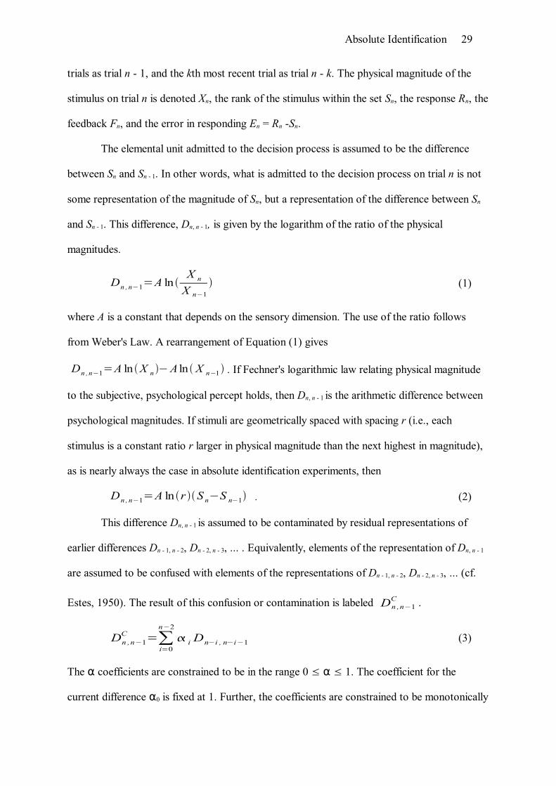
trials as trial n - 1, and the kth most recent trial as trial n - k. The physical magnitude of the

stimulus on trial n is denoted Xn, the rank of the stimulus within the set Sn, the response Rn, the

feedback Fn, and the error in responding En = Rn -Sn.

The elemental unit admitted to the decision process is assumed to be the difference

between Sn and Sn - 1. In other words, what is admitted to the decision process on trial n is not

some representation of the magnitude of Sn, but a representation of the difference between Sn

and Sn - 1. This difference, Dn, n - 1, is given by the logarithm of the ratio of the physical

magnitudes.

Dn , n�1=A ln �X n

X n�1� (1)

where A is a constant that depends on the sensory dimension. The use of the ratio follows

from Weber's Law. A rearrangement of Equation (1) gives

Dn ,n�1=A ln �X n ��A ln � X n�1 � . If Fechner's logarithmic law relating physical magnitude

to the subjective, psychological percept holds, then Dn, n - 1 is the arithmetic difference between

psychological magnitudes. If stimuli are geometrically spaced with spacing r (i.e., each

stimulus is a constant ratio r larger in physical magnitude than the next highest in magnitude),

as is nearly always the case in absolute identification experiments, then

Dn , n�1=A ln �r ��S n�S n�1� . (2)

This difference Dn, n - 1 is assumed to be contaminated by residual representations of

earlier differences Dn - 1, n - 2, Dn - 2, n - 3, ... . Equivalently, elements of the representation of Dn, n - 1

are assumed to be confused with elements of the representations of Dn - 1, n - 2, Dn - 2, n - 3, ... (cf.

Estes, 1950). The result of this confusion or contamination is labeled Dn ,n�1C .

Dn ,n�1C =�

i=0

n�2

� i Dn�i , n�i�1 (3)

The � coefficients are constrained to be in the range 0 � � � 1. The coefficient for the

current difference �0 is fixed at 1. Further, the coefficients are constrained to be monotonically


decreasing (i.e., �i > �i + 1), so that more recent differences are more likely to be confused with

the current difference. The idea that representations may be confused is quite ubiquitous in

psychology. What is unique in the RJM is the assumption that it is stimulus differences that are

confused, and this follows from our initial assumption that it is stimulus differences rather than

absolute magnitudes that are elemental. That is, Dn ,n�1C can be considered the result of a

confusion of stimulus differences in exactly the same way as any other representations might

be confused.

To produce a response, the difference Dn ,n�1C is converted to a difference on the

response scale by dividing by a constant �. (� represents the subjective size of the difference

that corresponds to a single unit on the response scale; see Luce & Green, 1974, and Marley,

1976, for a similar approach in magnitude estimation.) The result is then added to the feedback

from the previous trial (cf. Holland & Lockhead, 1968). It is at this point that we assume that

there is a limit in channel capacity. Next we outline the form that this limit takes in the RJM.

The limit in the channel capacity in the RJM is assumed to arise from noise in mapping

the stimulus difference onto the response scale. Lacouture and Marley (1995, 2004), Marley

and Cook (1984, 1986), and Petrov and Anderson (in press) also assume that the limit in

channel capacity is (at least partly) a result of noisy mapping. These authors give detailed

mechanistic accounts of the mapping process: in terms of a limited capacity rehearsal of the

context in a Thurstonian model (Marley & Cook, 1984, 1986); in terms of noisy activation of

a single connectionist unit (Lacouture & Marley, 1995, 2004); or in terms of exemplars

competing for selection (Petrov & Anderson, in press). Here we do not choose between these

accounts or offer our own mechanistic account. Instead we borrow a general principle from all

of these accounts. In each account, as the number of response categories is increased, fixed

magnitude noise in the mapping process leads to greater confusion between response

categories. For example, in Lacouture and Marley's mapping model, stimulus magnitudes are

represented by the activation of a hidden unit in a connectionist network. The activation of the


hidden unit varies between 0 and 1. Fixed magnitude noise is added to the activation of the

hidden unit. In experimental blocks where the set size is larger and, thus, the spacing of stimuli

on the hidden unit's unit interval is closer, the fixed magnitude noise causes greater confusion

between response categories. In the RJM, we make the additional assumption that, on a given

trial, some responses can be ruled out because of knowledge of Fn - 1 and the sign of Dn ,n�1C .

The limited capacity is then used to represent only the remaining responses. For example, if Sn

is perceived as being less than Sn - 1, then only those responses less than Fn - 1 are represented. If

Sn is greater than Sn - 1, then only those responses greater than Fn - 1 are represented. This

assumption follows directly from the initial assumption that judgment is relative.

We assume that the noise in the mapping process is normally distributed with variance

�2, and that this variance will be constant from trial to trial (and also from experiment to

experiment). However, as we outlined above, the effect of this noise on responding will not be

constant from trial to trial because the number of candidate responses will vary from trial to

trial. Consider the example illustrated in Figure 8A for the absolute identification of 10 stimuli.

If Sn - 1 = 4 and Sn = 8, then because Dn ,n�1C / 8 - 4 = +4 is positive, Rn must be higher

than Fn - 1 = 4. The response scale must now be partitioned into six responses (i.e., 5, 6, 7, 8, 9,

and 10). Compare this case with the case illustrated in Figure 8B. Now, Sn - 1 = 6 and, as

before, Rn must be higher than Fn - 1 = 6. Now, however, the same limited capacity can be used

to represent only four candidate responses (i.e., 7, 8, 9, and 10). In this latter condition, the

same variance noise in mapping translates into less confusion among responses, because the

limited capacity is partitioned into fewer response categories.

Two pieces of empirical evidence support this assumption. First, there is almost never

a problem deciding whether Sn is higher or lower than Sn - 1. In only 1.2% of the responses in

Experiment 1 (below) was the sign of the differences between consecutive stimuli mistaken

(i.e., responding with a higher number than Fn - 1 when Sn was lower in frequency than Sn - 1, and


vice versa). We describe the second piece of evidence in Experiment 2, which provides a

direct test of the assumption that Fn - 1 is used together with Dn ,n�1C in generating Rn.

Equation 4 implements the conversion of Dn , n�1C into a difference on the response

scale, and then the subsequent addition to Fn - 1 within a fixed limited capacity that is used to

represent the range of possible responses.

Rn=F n�1�Dn , n�1

C

��Z (4)

where Z is a normally distributed random variable that represents the noise in the mapping

process with a mean of 0 and a standard deviation of �, and � represents the range of possible

responses (given the sign of Dn ,n�1C and Fn - 1) and scales the fixed noise within the limited

capacity onto the response scale. Thus Rn is a normally distributed random variable. � is

specified exactly in Equation 5.

�={N�F n�1 if Dn , n�1C ��

1 if � �Dn , n�1C ��

F n�1�1 if Dn , n�1C �� } (5)

where N is the number of stimuli and � is a criterion whose magnitude Dn ,n�1C must exceed

for Sn and Sn - 1 to be assumed to be different. � is assumed to be fixed at half of the stimulus

spacing throughout this paper.

It is important to acknowledge here that Equations 4 and 5 do not represent a detailed

mechanistic account of how the difference between the current stimulus and the previous

stimulus is combined with the feedback from the previous trial to produce a response. We

simply intend Equations 4 and 5 to represent the assumption that a fixed magnitude noise in

the mapping process has a greater effect on trials where there are more candidate responses.

As we described above, the prediction that noise in the mapping process will increase as the

set size increases emerges from many accounts of absolute identification in which the mapping

process is specified in detail (e.g., Lacouture & Marley, 1995, in press; Marley & Cook, 1984,


1986; Petrov & Anderson, in press). In the RJM, we assume that, the noise varies not only

from block to block in an experiment as the set size is manipulated, but

also from trial to trial as the number of available responses varies (constrained by Fn - 1 and

Dn , n�1C ). In Equations 4 and 5, we assume that the noise in responding will grow linearly

with the number of available responses. We return to this issue later in this article, and suggest

that this simple assumption may need to be modified.

We assume that the location of the N - 1 criteria, labeled x1, x2, ..., xN - 1, that partition

the response scale is such that accuracy is maximized. The probability of a given response r is

given by the total density of Rn within the range

xr�1�Rn� xr (6)

with the lower and upper bounds replaced by -� and +� for the lowest and highest responses

respectively. Figure 9 shows the placement of criteria that maximizes the proportion of correct

responses for the parameters that best fit the data from Experiment 1. The dashed lines are

drawn at 1.5, 2.5, ..., 9.5. Notice that the optimal placement for criteria is more extreme than

criteria half way between integer values on the scale. This displacement is approximately a

linear function of the distance of the criteria xr from the center of the scale. (When predicting

the displacement of xr from r + 1 / 2 as a linear function of r, 99.96% of the variance is

accounted for.)

This outward displacement of optimal criteria happens because of a mathematical fact

proved by James and Stein (1961). James and Stein demonstrated that when predicting three

or more population means from three or more observations (one from each population), the

best estimate of each mean is not given by each observation. Instead, estimates derived by

shrinking each observation towards the grand mean of all the observations are better.4 Efron

and Morris (1977) provide an accessible introduction to James-Stein estimators, and give the

example of baseball players: The best estimate of a player's batting average in the next season

is not given by their score in the previous season. A better estimate is derived if their score is


shrunk towards the grand mean of all baseball players' scores. Here, we are trying to estimate

the correct response from a single noisy estimate (i.e., a single sample from Rn). James and

Stein's result tells us that the single sample from Rn will be too extreme compared to the mean

response. Thus, it is optimal to place the criteria at more extreme locations. Equation 7 gives

the location of each criterion.

xr=�R�r� 1

2��R

1�c(7)

where �R is the mean of the response scale (i.e., (N + 1) / 2) and 0 < c < 1 is a James-Stein

estimator. As c becomes larger, criteria are more outwardly displaced.

Fitting the RJM to Existing Data

In this section, we describe the mechanics of fitting the RJM to the data reviewed

above. The RJM has a set of � parameters that describe the confusion of the representations

of the differences between stimuli, a � parameter that scales between differences and response

scale units, a noise parameter �, and a James-Stein estimator c. For simplicity, the quantity 1 /

(A ln(r)) is absorbed into the � parameter. Thus, when � = 1, the size of the difference

between stimuli that corresponds to a single unit on the response scale is perfectly estimated. �

< 1 represents an underestimation of the stimulus spacing and � > 1 represents an

overestimation.

Except where specified otherwise, the data modeled in this section were collected from

experiments where a random sequence of stimuli was used. In modeling these data, the RJM

was used to generate predictions of the probabilities of each response for every possible

combination of the preceding and current stimuli. The relevant descriptive statistics were then

calculated as in the original experiments. For fits to these existing data sets, the MSE between

each data point and the predicted value was minimized. The best fitting parameter values were

found using both a downhill simplex procedure and Brent's method (Press, Flannery,

Teukolsky, & Vetterling, 1992). Fits were repeated with a large set of random starting values.


Best fitting parameters for each model are given in Table 3. Some data sets did not adequately

constrain all of the parameters. For example, in fitting the pattern of assimilation and contrast

in Figure 5, a wide range of � parameters was observed in the fits. When this happened, a fit

was chosen from the subset of fits with a MSE within 1% of the best fit MSE that had values

for the unconstrained parameters similar to those found in fitting other data sets.

The RJM Account of the Bow Effect

In Figure 2, a single fit is presented for all three stimulus spacing conditions in Brown

et al.'s (2002) experiment. The data did not constrain the � parameters for less recent stimuli,

and so a restricted version of the RJM with �3 = �4 = �5 = 0 was fitted. The RJM provides an

excellent fit to the characteristic bow.

The primary explanation for the bow effect is that there is a limited opportunity to

make errors at the end of the stimulus range. For example, Stimulus 1 can only be mistaken

for larger stimuli but Stimulus 5 can be mistaken for smaller or larger stimuli. However, given

that the error observed is normally only one, or maybe sometimes two response units (see, for

example, the confusion matrices in Figure 2), the restricted opportunity to make mistakes can

really only account for the peaks at each end of the accuracy against stimulus magnitude

curve, and does not offer an account of the gradual smooth curve over the entire stimulus

range.

The gradual bowing is accounted for because the effect of the limited decision capacity

is greatest for the central stimuli. When Sn lies in the center of the range, averaging over all

possible Sn - 1, the range of possible Rn constrained by Fn - 1 and Dn, n - 1 is, on average, larger than

when Sn lies at an extreme. For example, Table 4 shows the range of possible responses for

two cases, Sn = 1 and Sn = 5. Averaged over all possible Sn - 1, the range of possible responses

is smaller for the extreme stimulus. Thus, the differences leading to extreme stimuli can, on

average, be translated more accurately than differences leading to central stimuli within the

limited capacity. Optimal use of a limited capacity decision scale, then, acts to reduce accuracy


in the center of the range, more than it reduces accuracy at the edge of the range. Together

with the limited opportunity for errors at the edge of the range, the effects produce the

characteristic smooth bow.

A single set of parameters was used across all of the set sizes in fitting the bow effects

in accuracy in Lacouture and Marley's (1995) data (Figure 3). With only the set size differing

between fits, the RJM is able to provide a good account of the bows. A key observation is that

the limited capacity for representing the range of possible responses can represent two

possible alternatives nearly perfectly, but not many more. For this reason, the decision process

will not add noise in a task were two stimuli are identified but will add noise when there are

more than two stimuli. The RJM is able to account for the dependency of the bow effect on

set size because, as the set size increases, the average magnitude of both the differences

between stimuli and the range of possible responses on any given trial increases. Both of these

increases lead to more variability in responding.

A shortcoming of the RJM in its present instantiation is that it does not make

predictions about reaction times. Reaction times are faster for extreme stimuli (e.g., Kent &

Lamberts, in press; Lacouture & Marley, 1995). As described above, some models can predict

this effect (e.g., Lacouture & Marley, 1995; Nosofsky, 1997) and other models go further and

predict reaction time distributions for each stimulus (Karpiuk et al., 1997; Kent & Lamberts, in

press; Lacouture & Marley, 2004). Though we have not addressed this issue in this article, it

may be possible to extend the RJM to predict response time distributions. In its present form,

noise is added to the quantity F n�1�Dn ,n�1C / (see Equation 4) and the result Rn is

partitioned into response categories (see Equation 6) using fixed criteria. Instead of assuming

that response probabilities are given directly by the integrals of the probability density between

relevant criteria, a set of leaky competing accumulators (Usher & McClelland, 2001) could be

used (following Lacouture & Marley, 2004). By using Fn - 1 and the sign of Dn , n�1C to restrict


which accumulators from the full set (one for each response category) enter into the

competition on each trial, full response time distributions that are conditional upon the current

stimulus and previous stimuli could be predicted. Although it would be hard to test the fully

conditional distribution predictions because of the large amount of data required (e.g., for

absolute identification of 10 stimuli and sequence effects up to a lag of five trials, there would

be 106 possible sequences, each requiring of the order of 100 repetitions to construct full

reaction time distributions), this extension of the RJM could be tested with data conditional

upon, say, just the current stimulus.

The RJM Account of the Limit in Information Transmission

In modeling the limit in information transmitted (Figure 1), a single set of best fitting

parameters was used across all set sizes. Again, the data did not constrain the � parameters

for less recent stimuli, and so a restricted version of the RJM with �3 = �4 = �5 = 0 was fitted.

Dashed lines represent the fits to the Pollack (1952) and Garner (1953) data. Information

transmitted is completely defined by the confusion matrix. Thus, the RJM's account of the limit

in information transmitted as the number of stimuli is increased is the same as that given above

for the confusion matrix.

The RJM Account of the Restricted Sequence Designs

Fits of the RJM to Luce et al.'s (1982) proportion correct data are shown in Figure 6,

using a single set of parameters for all conditions. In fitting these data, the responses that the

RJM could generate on each trial were restricted to be those available to participants. There

were 10 criteria dividing the response scale into 11 categories positioned according to

Equation 7. However, in the small step (3) condition, for example, when each stimulus was

either one smaller than, the same as, or one larger than the previous stimulus, only the relevant

2 of these 10 criteria that divided the response scale into the categories Fn - 1 -1, Fn - 1, and Fn - 1

+ 1 were used.

As before, the data did not constrain the � parameters for less recent stimuli, and so a


restricted version of the RJM with �3 = �4 = �5 = 0 was fitted. The RJM fits the bow effect in

mean proportion correct and orders the sequences correctly. Within the RJM, the advantage

for conditions with smaller transitions results from the cumulative effect of the smaller

transitions, in agreement with Nosofsky (1983a) and Luce et al.'s (1982) conclusions. With

smaller transitions, because the range of previous stimuli will be smaller, Dn ,n�1C is less

variable (Equation 3). Together with reduced noise in the mapping process when a stimulus is

repeated (Equations 4 and 5), with is more likely with smaller transitions, these two properties

of the RJM give higher accuracy for sequences with smaller transitions. (As we noted in the

initial presentation of Luce et al.'s data, accuracy is higher in the large step condition than the

random condition, because the responses available on each trial are restricted in the large step

condition. However, performance measured by d' is higher for the random step condition than

the large step condition. Immediately below, we show that the RJM predicts this.)

The RJM Account of Bows in Discriminability

Using the parameter set from fitting the accuracy data (above), we also generated

predictions for d' for Brown et al.'s (2002; our Figure 10) data, Lacouture and Marley's (1995;

our Figure 3) data and for Luce et al.'s (1982; our Figure 6) data. Parameters from the

accuracy fits were used because the optimization algorithm performed very poorly when fitting

d' directly. The RJM does predict bows in d' because the effect of the limited decision capacity

is greatest for central stimuli, as described above. However, the size of this effect is

systematically underestimated. The RJM predicts that the confusion between the lowest two

stimuli and also between the highest two stimuli is larger than is actually observed. Below, we

consider two modifications that should allow the RJM to predict better the bows in d'.

In the RJM, we assume that the limit in channel capacity is caused by fixed variability

noise in mapping between stimulus differences and the response scale. In Equation 4, we make

the perhaps overly simple assumption that the effect of this fixed mapping noise � on the

variability in responding on a given trial is a linear function of the number of available


responses � (see Equation 5). If one assumes a different relationship (specifically, a convex

relationship when the effect on the response scale is plotted against the range of possible

responses) then greater bows in d' can be predicted. Motivating the functional form of this

relationship will require more detailed assumptions about the procedural nature of the

mapping from stimulus differences to the response scale. Lacouture and Marley (1995, 2004)

assume that the limit results from the range of stimulus magnitudes being represented by the

activation of a single noisy unit in a connectionist network. Marley and Cooke (1984, 1986)

assume the limit in mapping arises because of a limited rehearsal capacity in maintaining the

context against which a stimulus is judged. Either one of these assumptions could be

incorporated into the RJM.

An alternative modification would be to assume that the edge stimuli are somehow

privileged, as other authors do (e.g., Braida et al., 1984; Marley & Cook, 1984, 1986;

Nosofksy 1997). For example, participants may utilize representations of the magnitude of the

extreme stimuli if they occur two or three trials ago which they do not utilize for interior

stimuli. Alternatively, maybe a limited number of long-term representations of absolute

magnitudes can be maintained, and the extreme stimuli are preferentially selected. Though

these assumptions would complicate the RJM, they may prove to be necessary in providing a

fuller account of the d' data.

The RJM Account of Assimilation and Contrast

Fits of the RJM to the sequential effects of Holland and Lockhead (1968), Lacouture

(1997), and Ward and Lockhead (1970) are shown in Figures 4 and 5. In the RJM, sequence

effects result from the confusion of the representation of the current difference with the

representation of other differences. The complex pattern of first assimilation and then contrast

emerges naturally from the RJM, as a consequence of the assumption that more recent

differences are more likely to be confused or contaminated with the current difference than

less recent differences are. Equations 2 and 3 may be substituted into Equation 4 to give


Rn=Fn�1�A ln �r�

[� 0�S n�Sn�1�� 1�Sn�1�S n�2�� 2�S n�2�S n�3��...]�� Z .

Recalling that, when feedback is provided, Fn - 1 = Sn - 1 rearranging by collecting together Sn - i

terms gives

Rn=A ln �r �

� 0 S n��1� A ln �r �

�� 1�� 0��S n�1�A ln �r�

�� 2�� 1� S n�2

� A ln �r�

�� 3�� 2� S n�3�...�� Z(8)

For assimilation of Rn to Sn - 1 to occur,

1� A ln �r �

�� 1�� 0 ��0 .

Given an approximately correct estimate of the stimulus difference corresponding to a single

unit on the response scale (i.e., � = A ln(r)) and recalling that the availability of the current

difference was set at �0 = 1, then this inequality reduces to �1 > 0. �1, which represents the

extent to which Dn - 1, n - 2 is confused with Dn, n - 1, is positive and so assimilation is predicted.

Assimilation is still predicted if � � A ln(r) unless � is greatly overestimated.

For contrast of Rn to Sn - 2 to occur,

A ln �r �

�� 2�� 1 ��0

(with similar expressions for less recent stimuli). Given that A ln(r) and � are both positive,

and that �1 > �2 (reflecting a greater confusion of Dn, n - 1 with Dn - 1, n - 2 than with Dn - 2, n - 3)

contrast is always predicted.

In summary, in the RJM, the awkward pattern of assimilation and then contrast follows

in a straightforward way from the assumption that the current difference is confused more

with more recent differences. To capture this pattern in a model where absolute stimulus

magnitudes are used would be difficult, because one would need to motivate a switch in the

sign of the coefficient for Sn -1 compared to Sn - 2, Sn - 3, ... .

The RJM Account of the Response Scale Shrinkage


The data in Figure 4 show that, irrespective of Sn - 1, if Sn is small it is overestimated

(i.e., En > 0) and if Sn is larger it is underestimated (En < 0). The RJM model accounts for this

pattern because optimally-located response criteria xr are spread outwards from the center of

the scale.

Extensions of the RJM

The Effect of Range

Thus far we have accounted for the key phenomena in absolute identification by

assuming that the locus of these effects lies purely in the response process. We have assumed

that the effects are not perceptual, because all of the effects are seen with very widely spaced

stimuli. When stimuli are already widely spaced, increasing their spacing does little to improve

performance (e.g., Brown et al., 2002). However, if stimuli are closely-spaced then increasing

their spacing does improve performance (e.g., Braida & Durlach, 1972; see our Figure 11), up

to an asymptotic limit. So, at least for closely-spaced stimuli, stimulus noise does play some

role in limiting performance in absolute identification. The version of the RJM presented above

cannot account for this result, because the RJM predicts no effect of increasing the range of

the stimuli. Because of the ratio in Equation 1, the RJM is scale free (Chater & Brown, 1999).

That is, the magnitude of all of the stimuli could be increased by any factor and the same

predictions would be made (see Lacouture, 1997, for an empirical demonstration). However,

it is straightforward to extend the model to include a stimulus noise component by replacing

Equation 1 with

Dn ,n�1=A ln �X n

X n�1� (9)

where stimulus magnitudes are now random variables. Substituting Equation 9 into Equation 3

gives

Dn ,n�1C =� 0 A ln X n�� 1�� 0�A ln X n�1�� 2�� 1�A ln X n�2�... .

Thus Dn ,n�1C is also a random variable, which we assume to be normally distributed (which


follows from assuming that the distribution of the logarithm of stimulus magnitudes is normal)

with standard deviation �s. This version of the model can account for the data in Figure 11

using a single parameter set for all stimulus ranges (�1 = 0.271, �2 = 0.253, c = 0.109, � =

0.025, � = 0.892, and �s = 0.129).

Even with this modification there are still some data that are problematic for the RJM.

Nosofsky (1983b) investigated whether stimulus noise or criteria noise was increased when

the stimulus range was increased in absolute judgment of the intensity of tones. By fitting a

simple Thurstonian model Nosofsky found evidence that both stimulus and criterial noise

increased with range. In its present form, the RJM does not predict an increase in stimulus

noise and would require a further assumption, such as a limit in the width of an attention band

(cf. Luce et al., 1976).

Designs with Uneven Stimulus Spacing

Stimuli are not always evenly spaced in absolute identification designs. For

example,Lockhead and Hinson (1986) investigated performance in an absolute identification

of three tones differing in intensity. They used three different stimulus sets. In the even-spread

condition, stimuli were evenly spaced at 58, 60, and 62 dBA. In the low-spread condition, the

lowest stimulus was 4 dB less intense (i.e., a set of 54, 60 and 62 dBA intensities). In the high-

spread condition, the highest stimulus was 4 dB more intense (i.e., a set of 58, 60, and 66 dBA

intensities). Figure 12 gives the confusion matrices for each condition. Comparing the low-

and even-spread conditions, it can be seen that identification performance of the common

stimuli (Stimuli 2 and 3) is affected by the location of Stimulus 1. Stimuli 2 and 3 are more

likely to be confused when Stimulus 1 is lower. A similar (mirror image) pattern is seen when

the the high- and even-spread conditions are compared.

The RJM can capture this pattern. Because stimuli are no longer evenly spaced, we

have not used Equation 7 to place criteria. Instead, we have left the criteria as free parameters.

In the even condition, we introduced the constraint x2 = 4 - x1, to ensure that x2 is displaced


away from the center of the scale in exactly the same way as x1. (Although parameterized

slightly differently, this model is exactly equivalent to the RJM described in the Mathematical

Specification.) In the low and high spread conditions, x1 and x2 were allowed to vary freely,

with the constraint that there was symmetry between the low and high spread conditions (i.e.,

x1, low = 6 - x1, high and x2, low = 6 - x2, high). Figure 12 shows the best fits that minimize MSE

between the data points and the model predictions (� = 0.073, � = 0.373, � = 0.285, x1, even =

0.578, x1, low = 1.047, x2, low = 5.886). The model fits the data reasonably well (r2 = .98).

Comparing the low-spread and even conditions, the model correctly predicts that Stimuli 2

and 3 are more likely to be confused when Stimulus 1 is low. Comparing the high-spread and

even conditions, the model correctly predicts that Stimuli 1 and 2 are more likely to be

confused when Stimulus 3 is high. (Deviations of the data from model predictions are mainly

caused by a lack of symmetry in the data. For example, in the data for the even condition,

Stimulus 2 is responded to with 3 more often that 1, suggesting that stimuli were not exactly

evenly spaced psychologically.)

The Effect of Omitting Feedback

The RJM relies upon the previous feedback in generating a response (see Equation 4).

Here we extend the RJM to situations where feedback is omitted. Omitting feedback also

alters the sequential effects in absolute identification. When feedback is omitted, information

transmitted from the previous response increases, and information transmitted from the

previous stimulus is reduced (Mori & Ward, 1995). Note that, in this task, Mori and Ward

held accuracy constant across the feedback and no-feedback conditions. The change in

sequential effects is thus not due to an overall change in accuracy or task difficulty. In addition

to the change in the pattern of information transmission, assimilation, rather than contrast, is

observed to stimuli further back in the sequence, and the effect of previous responses is

greater than the effects of previous stimuli (see Lockhead, 1984, for a review).

In the RJM, an estimate of the difference between the current and previous trials is


used together with the feedback from the previous trial to generate a response (see Equation

4). In the absence of feedback, we assume that participants use their response from the

previous trial as the best estimate of the correct answer on the previous trial (i.e., Fn - 1 is

replaced with Rn - 1 in Equation 4). To test this assumption, we ran 100,000 simulated trials of

an absolute identification of 10 stimuli using the RJM with the best-fitting parameter values for

the data from Experiment 1. Following Mori and Ward's (1995) design, the presence of

feedback was alternated every 20 trials (i.e., 20 trials with feedback followed by 20 trials

without feedback). We then calculated the amount of information transmitted from the

previous stimulus and from the previous response to the current response separately for

feedback and no-feedback trials (see Table 5). Consistent with Mori and Ward's finding, when

feedback was omitted, the amount of information transmitted from the previous response was

increased and the amount of information transmitted from the previous stimulus was reduced.

We also examined sequential effects separately for feedback and no-feedback trials (see Figure

13). Again, consistent with experimental results (Lockhead, 1984), we found that assimilation

at larger lags, instead of contrast, was observed when feedback was omitted. In summary, the

assumption that participants use their previous response as the best estimate of the correct

answer in the absence of feedback and then proceed with a relative judgment strategy

correctly predicts the effects of omitting feedback.

Experiment 1

Whilst the RJM is able to provide an account of all of the main phenomena described

above, there are no raw data available that will allow these effects to be simultaneously

observed and modeled. It is possible, therefore, that whilst the RJM can provide an account of

each effect in isolation, the relative sizes of the effects may be such that they cannot be

simultaneously modeled. For this reason, a standard absolute identification of frequency

experiment was run to provide the raw data necessary to rule out this possibility. Two

stimulus spacings were crossed with three set sizes to produce six conditions.


Method

Participants. One hundred and twenty University of Warwick undergraduates

participated in this 45-minute experiment for course credit or payment of £5 (approximately

U.S. $8). Participants had at most one previous experience of an absolute identification of

frequency experiment.5

Stimuli. Stimuli were two sets of 10 tones varying in frequency. In the wide-spacing

condition, the lowest tone had a frequency of 600.00 Hz, with each subsequent tone increasing

in frequency by 12%. Thus the wide tones had a total range of 1063.85 Hz. In the narrow-

spacing condition, the lowest tone had a frequency of 768.70 Hz, with each subsequent tone

increasing in frequency by 6%. Thus, the total range in the narrow condition was 530 Hz.

Because, in both conditions, frequency increased by a constant percentage, tones were equally

spaced in log space, and were intended to be approximately evenly spaced psychologically.

The center of the range of the wide spacing condition coincided with the center of the range of

the narrow condition in log space (i.e., in each condition the tones had the same geometric

mean). In the set-size-8 conditions, only the middle 8 tones were used. Similarly in the set-

size-6 conditions only the middle 6 tones were used.

Each tone was 500 ms in duration, with the beginning 50 ms ramped linearly from

silence to maximum amplitude, and the end 50 ms ramped linearly from maximum amplitude

to silence.

Design. Two factors were varied between participants: (a) the spacing of the tones

was narrow or wide; and (b) the set size was 6, 8, or 10 stimuli. These two factors were

crossed producing six conditions. Participants were assigned to each condition at random,

with the constraint that there were an equal number of participants in each condition.

Procedure. Participants were tested individually in a quiet room. Participants

experienced seven blocks of 120 tones, with each tone occurring equally often in each block.

The ordering of the tones within a block was random. The breaks between blocks were self


timed by participants. Tones were delivered to participants using Sennheiser eH2270

headphones. The headphones were of high quality to ensure that tones sounded approximately

equally loud over the entire frequency range. At the same time as the tone was played, a "?"

prompt appeared on the screen until participants responded. Participants were free to respond

from the onset of each tone using the number keys along the top of a standard keyboard.

Other key presses were ignored. For half of the participants in each cell, tones were numbered

from lowest to highest and, for the other half of the participants, this mapping was reversed.

Participants were told that each tone was one of a set of 6, 8, or 10 varying in

frequency, and the ordering of the responses (either low numbers for low stimuli and high

numbers for high stimuli, or vice versa). Immediately after their response, the prompt was

removed and the correct answer was displayed on the screen for 750 ms. There was a silent

pause and blank screen for a duration of 500 ms before the next trial began automatically.

Results

As sequence effects in absolute identification are of concern here, data from the first

10 trials in every block were excluded from analysis so that only data where participants are

some way into the sequences are considered. The descriptive statistics presented were

calculated for each participant and then averaged across participants.

Average Accuracy. For each of the six cells in the design (three set sizes x two

stimulus spacings), the proportion of correct responses made by each participant was

calculated. Participants whose proportion was more than two inter-quartile ranges above the

upper quartile or below the lower quartile were to be excluded as outliers. In fact, only one

participant in the narrow-spacing-set-size-6 cell was eliminated from subsequent analysis (their

accuracy was too low).

To test out intention that stimuli would be evenly psychologically spaced, average

accuracy on the lower pitched half of the stimuli was compared to average accuracy on the

higher pitched half of the stimuli. There was a significant, t(118) = 5.07, p < .0001, but small


(3%) accuracy advantage for higher pitched stimuli. This suggests that stimuli were not quite

psychologically evenly spaced, but that higher pitched stimuli were more widely spaced. To

remove this asymmetry from the data in the following analyses data were collapsed across

mapping (so that Stimulus 1 was the lowest pitched for half of participants and highest pitched

for the other half).

Figure 14 shows how the proportion of correct responses varied through the

experiment for each cell of the design. Accuracy was higher for the smaller set sizes, and for

the wider stimulus spacings. Accuracy also improved slightly over blocks. This description of

results is confirmed by a three-way ANOVA, with three levels of set size (6, 8, and 10), two

levels of stimulus spacing (narrow and wide), and seven levels of block. All of the main effects

were significant: set size, F(2, 113) = 45.98, p < .0001; stimulus spacing, F(1, 113) = 11.13, p

= .0012; and block, F(6, 678) = 26.47, p < .0001. None of the interactions were significant.

In the remainder of this analysis, only data from the last five blocks were used, where

performance is approximately at asymptote. Using data from all blocks gives a very similar

pattern of results.

Information Transmitted. Table 6 shows the average information transmitted from

stimulus to response. Information transmitted is approximately constant across set sizes, and

increases with spacing. This pattern is confirmed by a two-way ANOVA with spacing and set

size as factors. There was no main effect of set size, F(2, 113) = 0.49, p = .61. There was a

significant effect of spacing, F(1, 113) = 7.87, p = .0059. There was no significant interaction,

F(2, 113) = 0.39, p = .68.

Central Tendency in Responding. There was a significant central tendency in

responding. Figure 15 shows the proportion of times each response was used for each stimulus

spacing and set size. The significance was determined by fitting a quadratic to the proportions

for each participant. The coefficient of the squared term was, on average, significantly below

zero, t(118) = 6.77, p < .0001.


In addition to the central tendency in responding, there was a tendency for people to

press the keys on the right of the keyboard more than those on the left. However, as the

assignment of response numbers to keys was counterbalanced across participants, this

tendency is not seen in the averaged data.

Bow in the Serial Position Curve. The proportion of correct responses is plotted

against stimulus for each stimulus spacing and set size in the top panel of Figure 16. Separate

two-way ANOVAs (stimulus x spacing) were run for each set size. For set size 10, there was

a main effect of stimulus, F(9, 342) = 59.19, p < .0001 (Huynh-Feldt � = .86), no main effect

of spacing, F(1, 38) = 1.72, p = .19, and a significant stimulus x spacing interaction, F(9, 342)

= 2.67, p = .0052. For set size 8, there was a main effect of stimulus, F(7, 266) = 93.34, p < .

0001 (Huynh-Feldt � = .93), no main effect of spacing, F(1, 38) = 1.30, p = .26, and no

significant stimulus x spacing interaction, F(7, 266) = 1.44, p = .20. For set size 6, there was a

main effect of stimulus, F(5, 185) = 43.16, p < .0001 (Huynh-Feldt � = .94), a main effect of

spacing, F(1, 37) = 7.81, p = .0082, and no significant stimulus x spacing interaction, F(5,

185) = 0.92, p = .47. Although the effect of spacing was only significant for set size 6, we

have already seen that there was a significant main effect of spacing on accuracy (see Average

Accuracy).

The bottom panel in Figure 16 plots bows in d'. Again, separate two-way ANOVAs

were run for each set size. Each of these revealed a main effect of spacing, smallest F(8, 304)

= 3.88, p < .0001. There was a marginal main effect of spacing for set size 6, F(1, 37) = 1.85,

p = .06. The effect was not significant for set sizes 8 and 10, larger F(1, 38) = 1.85, p = .18.

There was a significant interaction between stimulus and spacing for set size 10, with smaller

edge effects in the larger set size, F(8, 304) = 3.89, p = 0.0002. The interaction was not

significant for set sizes 6 or 8, larger F(6, 288) = 1.48, p = .18.

Figure 17 plots the confusion matrices for each of the six cells in the design (3 set sizes

x 2 spacings).


Assimilation and Contrast. Figure 18 plots En as a function of the Sn - 1 for different Sn.

There is a tendency for the responses to small stimuli to be too large, and for the responses to

large stimuli to be too small, as shown by the spacing of the lines. The positive slope of the

lines indicates that the response given to Sn is biased towards Sn - 1 (i.e., assimilation). Six

ANOVAs were run to confirm this description, one for each cell in the design (3 set sizes x 2

stimulus spacings). In every ANOVA, there was a significant main effect of Sn, a significant

main effect of Sn - 1, and no significant interaction.

Figure 19 plots En (averaged over all possible stimuli) against the lag k for different Sn -

k. When Sn - 1 (k = 1) is large, a positive error is made, and when Sn - 1 is small a negative error is

made (i.e., assimilation). For trials further back, the opposite pattern is seem (i.e., contrast).

When k = 2, the error dependency is small, showing that the stimulus two trials ago is having

little effect on responding. Six ANOVAs were run to confirm this description, one for each

cell in the design (3 set sizes x 2 stimulus spacings). Apart from the two set size 8 conditions,

there was no main effect of Sn - k. Apart from the two set size 6 conditions, there was no main

effect of lag, k. Importantly, in every ANOVA there was a significant interaction.

Discussion

Experiment 1 has replicated the standard findings described in the Introduction,

demonstrating that all of the effects can occur simultaneously. As set size increased

information transmitted remained constant. This limit is below that observed for absolute

identification of pitch observed by Hartman (1954) and Pollack (1952), but approximately the

same as that observed by W. Siegel (1972). (Hartman used very large inter-trial intervals and

Pollack played white noise between each trial.) We found a significant tendency for

participants to respond with responses in the center of the scale (see also Balakrishnan, 1997).

The bow in the serial position curve was shown in every condition. With larger set sizes, the

bow effect is larger (replicating the findings of Alluisi & Sidorsky, 1958; Durlach & Braida,

1969; Lacouture & Marley, 1995; Pollack, 1953; and Weber et al., 1977), and doubling the


spacing of the stimuli has only a slight effect on accuracy (replicating the findings of Braida &

Durlach, 1972; Brown et al., 2002; Lacouture, 1997; Luce et al., 1976; and Pollack, 1952).

For the larger two set sizes (8 and 10 stimuli), increasing the spacing did not improve accuracy

significantly, and the actual magnitude of the improvement was slight, if any. This is consistent

with Brown et al.'s (2002) findings. The bow effect was evident in every condition even in the

last block of this experiment, consistent with previous findings where the bow remains even

after extensive practice (Weber et al., 1977; Rouder et al., 2004).

The standard sequential effects were also evident in these data. The current stimulus

was assimilated towards the preceding stimulus (replicating the findings of Garner, 1953;

Holland & Lockhead, 1968; Hu, 1997; Lacouture, 1997; Lockhead, 1984; Long, 1937; Luce

et al., 1982; Purks et al., 1980; Rouder et al., 2004; Staddon, et al., 1980; Stewart, 2001; and

Ward & Lockhead, 1970, 1971). Rn was also contrasted away from earlier stimuli (replicating

the findings of Holland & Lockhead, 1968; Lacouture, 1997; and Ward & Lockhead, 1970,

1971). Though Holland and Lockhead found the contrast effect to be biggest for Sn - 2, these

data show greatest contrast for stimuli three or four trials back. This pattern is more consistent

with Lacouture's data, though perhaps slightly more extreme. Unpublished data from our

laboratory suggest that the spacing between trials is likely to be an important factor in

accounting for this difference.

In summary, each of the three main types of phenomena reviewed in the introduction -

the limit in information transmitted, bow in the serial position curve, and sequential effects -

have been demonstrated simultaneously in this experiment.

Modeling

A single fit to average data. As a proof of concept, we fitted the RJM to the average

data presented above. The purpose of the modeling described below is to demonstrate that the

RJM can fit the main phenomena accurately for a single set of parameter values. We took the

slightly ad-hoc strategy of minimizing the SSE between the data points presented in Figures


15, 17, 18, and 19, and the RJM's fits to these data points. The choice of how the SSEs from

each figure are combined is necessarily quite arbitrary as the SSEs for different figures are the

SSEs of quite different things (probabilities and errors on the response scale). However, the

exact weightings (1.0, 1.0, 0.1, and 0.5 for Figures 15, 17, 18, and 19 respectively) are not

important as very similar best fits are obtained for different weightings.

The RJM does not predict an effect of changing the spacing of the stimuli in the set. In

Experiment 1, there was a significant effect of spacing for only the smallest set size. For this

reason, the RJM was fitted to data for each set size averaged across the two different stimulus

spacings. We present one fit (see Table 3 for parameter values) as the dashed lines in Figures

20-24. r2 values for response biases, confusion matrices, assimilation plots and assimilation

and contrast plots were .98, .98, .89, and .94 respectively. Fits to d' data were poorer (r2 = .

88), and the RJM systematically under predicts the bow in the d' data, as described above.

Fits to individual participant's data. The purpose of Experiment 1 was to demonstrate

that the main phenomena occur simultaneously. This was observed above in the data averaged

across participants. Of the 119 participants, 100 showed bows in the proportion of correct

responses plotted against stimulus rank (as defined by greater average accuracy on edge

stimuli compared to internal stimuli) and assimilation to the previous stimulus and contrast to

those further back (as define by the coefficients of the simple regression model Rn = a0 Sn + a1

Sn - 1 + a2 Sn - 2 + ...) simultaneously.

To fit the RJM to the data from a single participant, we maximized the likelihood of

the model generating the data produced by the participant. The best fitting RJM predicts a

bow in accuracy, assimilation to the previous stimulus, and contrast to stimuli at greater lags

for every participant. When the predictions for the RJM are generated for each participant,

and then averaged across the participants in each condition, plots almost identical to those

obtained from fitting the averaged data are obtained. The median best fitting parameter values

across participants are given in Table 7, together with the upper and lower quartiles. These


values are very similar to those obtained above in fitting the averaged data (and so we do not

include them here).

In summary, the average data fit and the individual participant fits provide an existence

proof, demonstrating that the RJM is able to provide a good account of all of the main

phenomena simultaneously.

A Discrepancy: Conditional Accuracy and d'

There is a discrepancy in the literature that we have deferred discussion of until after

we had presented Experiment 1. W. Siegel (1972) found that accuracy was much higher when

the current stimulus was a repetition of the previous stimulus (see also Petrov & Anderson, in

press; Rouder et al., 2004). In the panels of Figure 25 we plot the bow effect for three

different set sizes. The effect is parameterized by the number of stimuli that intervened since

the current stimulus was last repeated. When a stimulus is repeated immediately accuracy is

practically perfect. With one intervening stimulus performance drops considerably and further

intervening stimuli lead to a smaller further drop. This pattern can be fit by the RJM. When a

stimulus is repeated Dn, n - 1 = 0 and, according to Equations 3 and 4, only the confusion of

differences makes a small contribution to En. However, when Sn - 1 <> Sn, then Dn, n - 1 <> 0 and

the limited decision capacity will add error to Rn. (The RJM fails to fit the difference between

one and more than one trial intervening between repetitions. This is because, as a first

approximation, we have assumed no memory for magnitudes other than Sn - 1. Modifying the

model to allow for some memory of Sn - 2 allows the model to predict the effect. Stewart and

Brown, 2004, found this modification necessary for modeling unidimensional categorization

data.)

In contrast, Purks et al. (1980), Luce et al. (1982), and Nosofsky (1983a) found that

there was only a small (though significant) increase in d' when, in a random sequence of

stimuli, the current stimulus was within one stimulus of the previous stimulus. There are

obvious explanations. First, the experiments used different stimuli. W. Siegel used tones


varying in frequency and Luce et al. and Purks et al. used tones varying in intensity. Second,

the performance measure is different. W. Siegel reports accuracy, Purks et al., Luce et al., and

Nosofsky report d'. Third, the partitioning of the data is different. W. Siegel used repetition

trials (i.e., Sn = Sn - 1), Purks et al. examined data for every combination of Sn and Sn - 1, and

Luce et al. and Nosofsky had stimuli differing by no more than 1 (|Sn - Sn - 1| � 1).

We have examined our own data from the narrow and wide set size 10 conditions of

Experiment 1. Consistent with W. Siegel's (1972) data, we found very high accuracy (> 98%

correct for every stimulus) on trials then the stimulus was repeated from the previous trial. We

also followed Luce et al.'s (1982) analysis and calculated accuracy and d' separately for trials

in the random sequence that were preceded by a stimulus no more than one different from the

current stimulus (near transitions) and trials that were more than one different from the

preceding stimulus (far transitions). Figure 26 shows our results. Unlike Purks et al., Luce et

al., and Nosofsky, we found a large advantage in accuracy and d' when the current and

previous stimuli were similar. This finding enables us to rule out the accuracy vs. d' difference

and the repetition vs. similar stimuli difference as explanations of the differences between the

experimental results, and suggest that the difference in findings is due to the use of different

stimuli (or other procedural differences). The finding of an d' advantage in the Experiment 1

data also enables us to rule out a response bias account of our accuracy data (and W. Siegel's

data), whereby the advantage for repeated stimuli comes from a strong tendency to repeat the

previous response. Instead, we think that the reduction in accuracy and d' found when the

previous and current stimuli differ occurs because stable, long-term magnitudes to which the

current stimulus can be compared are not available, and thus the current stimulus must be

compared to only the previous stimulus.

In Figure 26, we have shown the accuracy and d' predictions of the RJM using the

parameters from Table 3 for the Experiment 1 data. (Note that these parameters were not

chosen to best fit this pattern specifically.) The RJM predicts that accuracy and d' are higher


when Sn and Sn - 1 are similar because we assume that there is less noise in the mapping process

in this case (� is small when Sn = Sn - 1, see Equation 5).

At present, the RJM incorrectly predicts that a difference in accuracy and d' for the

Luce et al. (1982) random data (as we describe above for the Experiment 1 data). The RJM

could possibly be modified to correctly predict only a very small difference between accuracy

and d' in two ways. First, if the � parameter (which represents the magnitude below which

Dn , n�1C is so small that the Sn is considered a repetition of Sn - 1) were smaller, reflecting a

greater uncertainty in establishing whether a stimulus was a repetition, then accuracy and d'

would differ much less between the near and far conditions because the low noise mapping for

stimulus repetitions would occur less often. Alternatively, the preliminary form of Equation 5

could be altered. Further experimental work is required to constrain these possible extensions.

One question remains. If Luce et al. (1982) did not find an increase in d' or accuracy

when Sn is similar to Sn - 1 in their random condition, why is performance best in the small step

conditions which we described earlier? Nosofsky (1983) found evidence that the advantage

comes from the cumulative effect of a series of small transitions between consecutive stimuli

(rather than just a single small transition between Sn - 1 and Sn). Nosofsky took the trials where

Sn was no more than one stimulus different from Sn - 1 and partitioned the data further

depending on whether Sn - 2 was no more than one stimulus different from Sn - 1. Accuracy on

trial n was higher when Sn - 2 was more similar to Sn - 1. The RJM can account for this qualitative

pattern, because of the assumption that consecutive differences are confused (see Equation 3).

When Sn - 2 is more similar to Sn - 1, then, Dn , n�1C varies less, and thus responding is also less

variable.

Experiment 2

An important question is whether the RJM is falsifiable. We address this issue directly

in Experiment 2, which pits the predictions of absolute magnitude models (i.e., the


Thurstonian models, the restricted capacity models, and the exemplar models) and the RJM

against each other directly. The models make different predictions regarding the effect of

misleading feedback. In the RJM, the feedback from the preceding trial is used together with a

judgment of the difference between the preceding and current stimuli to produce a response. If

participants are given misleading feedback on the previous trial, then, according to Equation 4,

their response on the current trial should reflect this directly. In contrast, the absolute-

magnitude-based models described above do not use the feedback from the previous trial in

generating the response on the current trial, and so predict no effect of misleading feedback.

Below, we consider how, if the misleading feedback is attended to at all, the absolute-

magnitude-based models might use the feedback to adjust the mapping between the stimulus

scale and the response scale. Even with this adjustment, these models still make different

predictions from the RJM.

The experiment was designed such that performance on the final trial of eight critical

triplets of trials (defined by Sn - 2, Sn -1, Rn -1, Fn -1, and Sn ) could be compared in the analysis.

The triplets differed from one another in two ways. First, Fn - 1 could either be correct or

misleading. Second, Rn - 1 could either be correct or incorrect. Four of the triplets are listed in

Table 8. The remaining four triplets are the mirror image of the four listed in Table 8 (the

values of Sn - 2, Sn -1, Rn -1, Fn -1, and Sn for these mirror image triplets can be generated by

subtracting the values in Table 8 from 11 and �En predictions can be generated by swapping

the sign of the value in Table 8). In the remainder of this article, for simplicity of exposition,

we will discuss the triplets in terms of those listed in Table 8.

In each triplet, Sn - 2 was far from Sn - 1 so that, if Fn - 1 were misleading, the deception

would not be obvious. When Fn was too great by one, according to the RJM (see Equation 4),

En should also be too great by one (see the RJM �En column of Table 8). This prediction can

be tested by comparing the first two triplets in Table 8: En when Fn - 1 was misleading and En

when Fn - 1 was not misleading (to provide a baseline measure of the bias due to assimilation


and contrast).

However, under the alternative assumption that judgment is absolute, there is an

alternative explanation of an increased error when Fn - 1 is misleading. Suppose that, upon

being told that their response was incorrect, the participant adjusts their mapping of stimuli to

responses. If their response was too small by one, then responses should be remapped onto

stimuli so that each stimulus is now mapped onto the response that previously belonged to the

next highest stimulus. For example, in a Thurstonian model (e.g., Durlach & Braida, 1969;

Luce et al., 1976; Treisman, 1985), all of the criteria should be shifted down the perceptual

scale by one stimulus spacing. In an exemplar model (e.g., Brown et al., 2002; Kent &

Lamberts, in press; Nosofsky, 1997; Petrov & Anderson, in press), each exemplar should be

remapped so that it is associated with the label that was originally associated with the

immediately higher exemplar. Thus, after the misleading feedback that is too large by one,

each stimulus will now be associated with a response that is also one too large (see the

Mapping En column of Table 8).

Though the RJM and the mapping alternative make the same predictions when Rn - 1 is

correct, they make different predictions when Rn - 1 is incorrect (see the last two triplets listed

in Table 8). Take, for example, the case illustrated in the third row of Table 8. Within a

Thurstonian framework, if the perception of Sn - 1 = 4 is noisy so that the percept falls below

the criteria between response categories 3 and 4, then Rn - 1 will be incorrectly underestimated

as 3. Truthful feedback (i.e., Fn - 1 = 4) will indicate that an error has been made, and criteria

might be adjusted in response by shifting them one unit down the response scale. Now, when

Sn = 6 is presented, Rn will be an overestimate. The same argument can be made for an

exemplar framework. If perception of Sn - 1 = 4 is noisy so that the percept is more similar to

the exemplar for category 3 than category 4, then Rn - 1 will be incorrectly underestimated as 3.

Truthful feedback (i.e., Fn - 1 = 4) will indicate that an error has been made, and the mapping

between exemplars and category labels should be adjusted so that each exemplar is now


mapped to the label previously belonging to the next highest exemplar. Now, when Sn = 6 is

presented, Rn will be an overestimate. When Fn - 1 is misleading and confirms a mistaken Rn - 1

(see the fourth row of Table 8), the match between response and feedback should mean that

the participant thinks no error has been made, and does not adjust their mapping. Thus, no

error is predicted in identifying Sn.

In summary, the RJM predicts an effect of misleading feedback. Absolute magnitude

models predict the same effect if one augments them with the ability to adjust the mapping

between stimuli and responses in response to an error. However, the RJM and these

augmented mapping models make different predictions in the case when the previous response

is wrong but misleading feedback suggests that it was correct.

Method

Participants. Twelve female and seven male students from the University of Warwick

aged between 19 and 32 years participated for payment of £6 (approximately U.S. $10).

Stimuli. Ten stimuli were generated. The first was 200 Hz, with a between-stimulus

spacing of 25%, giving a last stimulus of 1490 Hz. This spacing is just over twice the spacing

of the stimuli used in the wide condition of Experiment 1. The amplitude envelope applied to

the stimuli was that used in Experiment 1.

Design and Procedure. The procedure closely follows that of Experiment 1. There

were 20 blocks of 40 stimuli. Two of the eight critical triplets differ from another two only in

Rn - 1. Thus, there were only six unique critical triplets (ignoring Rn - 1, which, obviously, was

under the participants' control). In each block, these were randomly assigned to begin on trials

3, 10, 17, 24, 31, and 38. On the remaining trials, the stimulus was selected at random with

the constraint that all stimuli appeared equally often in each block. Feedback was always

correct, apart from on the middle trial of two of the six triplets, and thus feedback was only

misleading on 5% of trials.

Results


Figure 27 shows En as a function of whether Fn - 1 was correct or misleading,

parameterized by the accuracy of Rn - 1 (see Table 8 for a full description of the conditions). En

with Fn - 1 and Rn - 1 correct (as in a standard absolute identification experiment) is negative,

showing that Rn is assimilated towards Sn - 1 and contrasted away from Sn - 2. When Fn - 1 is

misleading (Fn - 1 = Sn - 1 + 1) then En is increased, as predicted by the RJM (and the mapping

hypothesis). The same pattern is seen when Rn - 1 is incorrect, as predicted by the RJM (the

opposite of the prediction of the mapping model). A two-way ANOVA (Fn - 1 correct or

misleading x Rn - 1 correct or incorrect) revealed a significant main effect of the accuracy of Fn -

1 [F(1, 18) = 20.84, p = .0002], no significant main effect of the accuracy of Rn - 1 [F(1, 18) =

0.31, p = .59], and no significant interaction [F(1, 18) = 2.95, p = .10]. Though the interaction

is approaching significance, it is in the opposite direction predicted by the mapping hypothesis.

The increase in En when Fn - 1 is too large by 1 was only .57 (averaged across the

accuracy of Rn). The RJM predicts that all of the increase in Fn - 1 should carry over to Rn.

However, we have already seen evidence that there may still be some residual memory for the

absolute magnitude of not just the preceding stimulus but also the stimulus before that (e.g.,

Massaro, 1970; W. Siegel, 1972; Stewart & Brown, 2004; Wickelgren, 1966). If Sn - 2 were

also used as an anchor against which to judge Sn then one would expect a smaller effect of Fn -

1 on En.

Information transmitted. The information transmitted in Experiment 1 was lower than

the estimates obtained by Pollack (1952) and Hartman (1954) for absolute identification of

pure tones varying in frequency. In Experiment 2, the spacing of the stimuli was greatly

increased compared to Experiment 1, but average information transmitted was 1.41 bits -

approximately the same as in Experiment 1 and W. Siegel (1972).

Discussion

According to the RJM, the difference between the current stimulus and the previous

stimulus is added to the feedback from the previous trial to generate the current response (see


Equation 4). Thus, the RJM makes the strong prediction that, if the previous feedback is

inaccurate, this error will be transmitted to the current response. In Experiment 2, we found

this to be the case. When participants were misled, and the previous feedback was one too

large, then the current response was significantly increased compared to when the previous

feedback was accurate.

Of all of the existing models of absolute identification, only Holland and Lockhead's

(1968) model, which makes the same assumption about the use of the previous feedback as

the RJM, can predict this effect. All of the other models fail to predict the effect in their

current forms, because they do not use the previous feedback in generating the current

response. Reasonable assumptions can be made to allow the models to adapt the mapping

between stimulus magnitudes and response categories after feedback indicates an error has

been made (e.g., shifting criteria in a Thurstonian model or relabeling exemplars in an

exemplar model). In this way, the models can predict that there will be an error on the current

trial when feedback on the previous trial is erroneous, because it will appear that an error has

been made on the previous trial and the model can alter the mapping between stimuli and

responses to compensate. However, the models then incorrectly predict that there will be no

effect of misleading feedback on the previous trial when the previous response was incorrect

but the (misleading) feedback indicates that it was correct. In this case, it will appear as if no

error has been made, and so no remapping should take place.

There is an alternative way that the absolute-magnitude-based models might be able to

account for the Experiment 2 data. Instead of perceptual noise being the cause of an incorrect

Rn - 1, Rn - 1 might be incorrect because the mapping between stimuli and responses is, for some

reason, already incorrect. For example, in the case illustrated in the last two rows of Table 8,

Rn - 1 might be underestimated because either Thurstonian criteria may be too far up a sensory

scale or because each exemplar might be mapped onto a label that is too low. Now, if Fn - 1 is

accurate and indicates an error, the adjustment of the mapping would correct the initial mis-


mapping. If Fn - 1 is misleading, and indicates no error when one has been made, then no

adjustment will be made. These predictions are now the same as those of the RJM. However,

in adopting this explanation though, the idea of relative judgment is incorportated. In assuming

that the mapping between stimuli and responses is adjusted after each piece of feedback and,

thus, varies from trial to trial, one is abandoning a stable long-term association between

particular magnitudes and response categories. There seems to be little difference between, on

the one hand, hearing a stimulus two higher than the previous stimulus and so responding with

a response two higher than the previous feedback and, on the other, hearing a stimulus and

aligning a response scale with it on the basis of the feedback and then hearing another stimulus

two higher and thus responding with a response two units up the response scale. In allowing

the continual adjustment of the mapping between the stimulus and the response scales, the

stable long-term mapping between absolute stimulus magnitudes and response categories is

abandoned and these models become models of relative judgment that are really rather similar

to the RJM proposed here.

Extending Relative Judgment Models

In this article, our core claim is that a model of relative judgment can provide an

account of many phenomena in the absolute identification literature. Our model differs from

existing models in assuming that long-term representations of absolute magnitudes are either

unavailable or, for some reason, are unused in absolute identification. Here, we outline three

ways in which this relative judgment idea might be extended.

The first way would be to test more directly the longevity of absolute magnitude

representations. Above, we cited ten reports of same-different judgment tasks in which the

memory for a standard decays rapidly as the interval until a comparison item is increased or

filled. However, in these experiments, the stimulus chosen as the standard varied from trial to

trial. With only one standard, there is little forgetting across intervening tones (D. A.

Anderson, 1914, as cited from Massaro, 1970, and Wickelgren, 1966; Irwin, 1937;


Magnussen, Greenlee, Aslaken, & Kildebo, 2003). We think an important step would be to

identify the conditions under which long-term representations of absolute magnitudes can and

cannot be maintained. The misleading-feedback methodology from Experiment 2 could also be

adapted to measure the longevity of absolute magnitude representations by remapping stimuli

and responses part way through an absolute identification experiment (e.g., by increasing the

feedback by one for the rest of the experiment) and measuring for how long the initial stimulus

response mapping persists. The effect of shifting the entire stimulus set between experimental

sessions (e.g., Ward & Lockhead, 1970; Ward, 1987) should also be investigated for other

stimulus continuums.

A second way in which the idea of relative judgment could be developed would be to

extend relative judgment approaches to other psychophysical tasks. We have already had some

success in modeling empirical results in unidimensional binary categorization (Stewart &

Brown, 2004; Stewart et al., 2002) that cannot be fit by existing absolute-magnitude-based

categorization models (e.g., the GCM, Nosofsky, 1986). Laming (1984, 1997) has been able

to account for some key results in magnitude estimation and cross-modality matching using his

relative judgment model.

Our final suggestion is that absolute and relative judgment models might be integrated

into a single theoretical framework. Obviously, at some level, in absolute-magnitude-based

models judgment is relative, because the information from previous stimulus-response pairings

provides the basis for generating each response. Also, at some level, relative judgment models

do assume that a (perhaps peripheral) representation of a stimulus's absolute magnitude can be

maintained in the very short term because, without such a representation over the inter-

stimulus interval, the following stimulus could not be compared to the previous stimulus. We

have already shown that our relative judgment model of unidimensional binary categorization

and an absolute-magnitude-based exemplar model (Nosofsky, 1986) are special cases of a

more general model (Stewart & Brown, 2005). That is, the relative judgment model can be


thought of as occupying one end of a continuum where absolute magnitude representations are

very short-lived, with the exemplar model occupying the other end, where absolute magnitude

representations are long-lived.

Conclusion

We have presented the RJM, in which, in the assumed absence of stable, long-term

absolute magnitudes, the representation of the difference between the stimulus on the current

trial and the stimulus on the preceding trial is used in conjunction with the feedback from the

previous trial to produce a response. We have demonstrated that a broad class of absolute

identification data can be fit by this model. Assuming relative judgment allows an account of

the ubiquitous sequential effects observed in absolute identification. By assuming only that the

representation of the difference between the current stimulus and the previous stimulus is

confused with the representations of earlier differences, the RJM predicts assimilation to the

previous stimulus and contrast to those stimuli further back. These effects have been

problematic for those existing models assuming that absolute identification is achieved using

long-term representations of absolute magnitudes of stimulus values (either as exemplars,

anchors, or criteria). Using difference information optimally within a limited capacity provides

an account of the bow effect and of the limit in information transmitted. We conclude,

therefore, that absolute identification may in fact be achieved by relative judgment.


References

Alluisi, E. A., & Sidorsky, R. C. (1958). The empirical validity of equal discriminability

scaling. Journal of Experimental Psychology, 55, 86-95.

Anderson, J. R. (1990). The adaptive character of thought. Hillsdale, NJ: Erlbaum.

Anderson, J. R., & Lebière, C. (1998). The atomic components of thought. Mahwah: NJ:

Lawrence Erlbaum Associates.

Ashby, F. G., & Townsend, J. T. (1986). Varieties of perceptual independence. Psychological

Review, 93, 154-179.

Bachem, A. (1954). Time factors in relative and absolute pitch determination. Journal of the

Acoustical Society of America, 26, 751-753.

Baird, J. C., Romer, D., & Stein, T. (1970). Test of a cognitive theory of psychophysics: Size

discrimination. Perceptual and Motor Skills, 30, 495-501.

Balakrishnan, J. D. (1997). Form and objective of the decision rule in absolute identification.

Perception & Psychophysics, 59, 1049-1058.

Beebe-Center, J. G., Rogers, M. S., & O'Connell, D. N. (1955). Transmission of information

about sucrose and saline solutions through the sense of taste. Journal of Psychology,

39, 157-160.

Braida, L. D., & Durlach, N. I. (1972). Intensity perception. II. Resolution in one-interval

paradigms. Journal of the Acoustical Society of America, 51, 483-502.

Braida, L. D., Lim, J. S., Berliner, J. E., Durlach, N. I., Rabinowitz, W. M., & Purks, S. R.

(1984). Intensity Perception. XIII. Perceptual anchor model of context-coding.

Journal of the Acoustical Society of America, 76, 722-731.

Brown, G. D. A., Neath, I., & Chater, N. (2002). A ratio model of scale-invariant memory

and identification. Manuscript submitted for publication.

Chapanis, A., & Halsey, R. M. (1956). Absolute judgments of spectrum colors. Journal of

Psychology, 42, 99-103.


Chater, N., & Brown, G. D. A. (1999). Scale-invariance as a unifying psychological principle.

Cognition, 69, b17-b24.

DeCarlo, L. T. (1992). Intertrial interval and sequential effects in magnitude scaling. Journal

of Experimental Psychology: Human Perception and Performance, 18, 1080-1088.

DeCarlo, L. T. (1994). A dynamic theory of proportional judgment: Context and judgment of

length, heaviness, and roughness. Journal of Experimental Psychology: Human

Perception and Performance, 20, 372-381.

DeCarlo, L. T., & Cross, D. V. (1990). Sequential effects in magnitude scaling: Models and

theory. Journal of Experimental Psychology: General, 119, 375-396.

Durlach, N. I., & Braida, L. D. (1969). Intensity perception. I. Preliminary theory of intensity

resolution. Journal of the Acoustical Society of America, 46, 372-383.

Efron, B., & Morris, C. (1977). Stein's paradox in statistics. Scientific American, 236,

119-127.

Elliott, S. W., & Anderson, J. R. (1995). Effect of memory decay on predictions from

changing categories. Journal of Experimental Psychology: Learning, Memory, and

Cognition, 21, 815-836.

Engen, T., & Pfaffmann, C. (1959). Absolute judgments of odor intensity. Journal of

Experimental Psychology, 58, 23-26.

Eriksen, C. W., & Hake, H. W. (1955a). Absolute judgments as a function of stimulus range

and the number of stimulus and response categories. Journal of Experimental


Eriksen, C. W., & Hake, H. W. (1955b). Multidimensional stimulus differences and accuracy

of discrimination. Journal of Experimental Psychology, 50, 153-160.

Eriksen, C. W., & Hake, H. W. (1957). Anchor effects in absolute judgment. Journal of


Estes, W. K. (1950). Towards a statistical theory of learning. Psychological Review, 57,


94-107.

Garner, W. R. (1953). An informational analysis of absolute judgments of loudness. Journal

of Experimental Psychology, 46, 373-380.

Garner, W. R. (1962). Uncertainty and structure and psychological concepts. New York:

Wiley.

Gravetter, F., & Lockhead, G. R. (1973). Criterial range as a frame of reference for stimulus

judgment. Psychological Review, 80, 203-216.

Green, D. M., & Swets, J. A. (1966). Signal detection theory and psychophysics. New York:

Wiley.

Hake, H. W., & Garner, W. R. (1951). The effect of presenting various numbers of discrete

steps on scale reading accuracy. Journal of Experimental Psychology, 42, 358-366.

Harris, J. D. (1952). The decline of pitch discrimination with time. Journal of Experimental


Hartman, E. B. (1954). The influence of practice and pitch-distance between tones on the

absolute identification of pitch. American Journal of Psychology, 67, 1-14.

Hawkes, G. R., & Warm, J. S. (1960). Maximum It for absolute identification of cutaneous

electrical intensity level. Journal of Psychology, 49, 279-288.

Helson, H. (1964). Adaptation-level theory. New York: Harper & Row.

Holland, M. K., & Lockhead, G. R. (1968). Sequential effects in absolute judgments of

loudness. Perception and Psychophysics, 3, 409-414.

Hu, G. (1997). Why is it difficult to learn absolute judgment tasks? Perceptual and Motor

Skills, 84, 323-335.

Irwin, C. C. (1937). A study of differential pitch sensitivity relative to auditory theory.

Journal of Experimental Psychology, 21, 642-652.

James, W., & Stein, C. (1961). Estimation with quadratic loss. Proceedings of the Fourth

Berkeley Symposium on Mathematics and Statistics, 1, 361-379.


Jesteadt, W., Luce, R. D., & Green, D. M. (1977). Sequential effects of the judgments of

loudness. Journal of Experimental Psychology: Human Perception and Performance,

3, 92-104.

Karpiuk, P., Lacouture, Y., & Marley, A. A. J. (1997). A limited capacity, wave equality,

random walk model of absolute identification. In A. A. J. Marley (Ed.), Choice,

decision and measurment: Essays in honor of R. Duncan Luce (pp. 279-299).

Mahwah, NJ: Erlbaum.

Kent, C., & Lamberts, L. (in press). An exemplar account of the bow and set size effects in

absolute identification. Journal of Experimental Psychology: Learning, Memory, and

Cognition.

Kinchla, R. A., & Smyzer, F. (1967). A diffusion model of perceptual memory. Perception

and Psychophysics, 2, 219-229.

König, E. (1957). Effect of time on pitch discrimination thresholds under several

psychophysical procedures: Comparison with intensity discrimination thresholds.

Journal of the Acoustical Society of America, 29, 606-612.

Lacouture, Y. (1997). Bow, range, and sequential effects in absolute identification: A

response-time analysis. Psychological Research, 60, 121-133.

Lacouture, Y., Li, S. C., & Marley, A. A. J. (1998). The roles of stimulus and response set

size in the identification and categorisation of unidimensional stimuli. Australian

Journal of Psychology, 50, 165-174.

Lacouture, Y., & Marley, A. A. J. (1991). A connectionist model of choice and reaction time

in absolute identification. Connection Science, 3, 401-433.

Lacouture, Y., & Marley, A. A. J. (1995). A mapping model of bow effects in absolute

identification. Journal of Mathematical Psychology, 39, 383-395.

Lacouture, Y., & Marley, A. A. J. (2004). Choice and response time processes in the

identification and categorization of unidimensional stimuli. Perception &


Psychophysics.

Laming, D. R. J. (1984). The relativity of "absolute" judgements. British Journal of

Mathematical and Statistical Psychology, 37, 152-183.

Laming, D. R. J. (1997). The measurement of sensation. London: Oxford University Press.

Lockhead, G. R. (1984). Sequential predictors of choice in psychophysical tasks. In S.

Kornblum & J. Requin (Eds.), Preparatory states and processes (pp. 27-47). Hillsdale,

NJ: Erlbaum.

Lockhead, G. R. (1992). Psychophysical scaling: Judgments of attributes or objects?

Behavioral and Brain Sciences, 15, 543-601.

Lockhead, G. R. (2004). Absolute judgments are relative: A re-interpretation of some

psychophysical ideas. Review of General Psychology.

Lockhead, G. R., & King, M. C. (1983). A memory model of sequential effects in scaling

tasks. Journal of Experimental Psychology: Human Perception and Performance, 9,

461-473.

Long, L. (1937). A study of the effect of preceding stimuli upon the judgment of auditory

intensities. Archives of Psychology (New York), 30, 209.

Luce, R. D., & Green, D. M. (1974). The response ration hypothesis for magnitude

estimation. Journal of Mathematical Psychology, 11, 1-14.

Luce, R. D., Green, D. M., & Weber, D. L. (1976). Attention bands in absolute identification.


Luce, R. D., Nosofsky, R. M., Green, D. M., & Smith, A. F. (1982). The bow and sequential

effects in absolute identification. Perception & Psychophysics, 32, 397-408.

Magnussen, S., Greenlee, M. W., Aslaken, P. M., & Kildebo, O. O. (2003). High-fidelity

perceptual long-term memory revisited - and confirmed. Psychological Science, 14,

74-76.

Marley, A. A. J. (1976). A revision of the response ration hypothesis for magnitude


estimation. Journal of Mathematical Psychology, 14, 252-254.

Marley, A. A. J., & Cook, V. T. (1984). A fixed rehearsal capacity interpretation of limits on

absolute identification performance. British Journal of Mathematical and Statistical


Marley, A. A. J., & Cook, V. T. (1986). A limited capacity rehearsal model for psychological

judgments applied to magnitude estimation. Journal of Mathematical Psychology, 30,

339-390.

Massaro, D. W. (1970). Retroactive interference in short-term memory for pitch. Journal of


McGill, W. J. (1954). Multivariate information transmission. Psychometrika, 19, 97-116.

McGill, W. J. (1957). Serial effects in auditory threshold judgments. Journal of Experimental


Medin, D. L., & Schaffer, M. M. (1978). Context theory of classification learning.

Psychological Review, 85, 207-238.

Miller, G. A. (1956). The magical number seven, plus or minus two: Some limits on our

capacity for information processing. Psychological Review, 63, 81-97.

Mori, S. (1998). Effects of stimulus information and number of stimuli on the sequential

dependencies in absolute identification. Canadian Journal of Experimental

Psychology-Revue Canadienne de Psychologie Experimentale, 52, 72-83.

Mori, S., & Ward, L. M. (1995). Pure feedback effects in absolute identification. Perception

& Psychophysics, 57, 1065-1079.

Murdock, B. B. (1960). The distinctiveness of stimuli. Psychological Review, 67, 16-31.

Nosofsky, R. M. (1983a). Shifts of attention in the identification and discrimination of

intensity. Perception & Psychophysics, 33, 103-112.

Nosofsky, R. M. (1983b). Information integration and the identification of stimulus noise and

criterial noise in absolute judgment. Journal of Experimental Psychology: Human


Perception and Performance, 9, 299-309.

Nosofsky, R. M. (1986). Attention, similarity and the identification-categorization

relationship. Journal of Experimental Psychology: General, 115, 39-57.

Nosofsky, R. M. (1997). An exemplar-based random-walk model of speeded categorization

and absolute judgment. In A. A. J. Marley (Ed.), Choice, Decision, and Measurement

(pp. 347-365). Hillsdale, NJ: Erlbaum.

Nosofsky, R. M., & Palmeri, T. J. (1997). An exemplar-based random walk model of speeded

classification. Psychological Review, 104, 266-300.

Norwich, K. H., Wong, W., & Sagi, E. (1998). Range as a factor in determining the

information of loudness judgments: Overcoming small sample bias. Canadian Journal

of Experimental Psychology, 52, 63-70.

Petrov, A. A., & Anderson, J. R. (in press). The dynamics of scaling: A memory-based anchor

model of category rating and absolute identification. Psychological Review.

Petzold, P., & Haubensak, G. (2001). Higher order sequential effects in psychophysical

judgments. Perception & Psychophysics, 63, 969-978.

Pollack, I. (1952). The information of elementary auditory displays. Journal of the Acoustical

Society of America, 24, 745-749.

Pollack, I. (1953). The information of elementary auditory displays. II. Journal of the

Acoustical Society of America, 25, 765-769.

Press, W. H., Flannery, B. P., Teukolsky, S. A., & Vetterling, W. T. (1992). Numerical

recipes in C : The art of scientific computing. New York: Cambridge University Press.

Purks, S. R., Callahan, D. J., Braida, L. D., & Durlach, N. I. (1980). Intensity perception. X.

Effect of preceding stimulus on identification performance. Journal of the Acoustical

Society of America, 67, 634-637.

Rouder, J. N., Morey, R. D., Cowan, N., & Pfaltz, M. (2003). Learning in a unidimensional

absolute identification task. Psychonomic Bulletin & Review, 11, 938-944.


Sagi, E., Wong, W., & Norwich, K. H. (2001). Mathematical studies of the information in the

stimulus response matrix. Journal of Mathematical Psychology, 45, 99-114.

Siegel, W. (1972). Memory effects in the method of absolute judgment. Journal of


Siegel, J. A., & Siegel, W. (1972). Absolute judgment and pared-associate learning: Kissing

cousins or identical twins? Psychological Review, 79, 300-316.

Shiffrin, R. M., & Nosofsky, R. M. (1994). Seven plus or minus two: A commentary on

capacity limitations. Psychological Review, 101, 357-361.

Staddon, J. E. R., King, M., & Lockhead, G. R. (1980). On sequential effects in absolute

judgment experiments. Journal of Experimental Psychology: Human Perception &

Performance, 6, 290-301.

Stevens, S. S. (1975). Psychophysics. New York: Wiley.

Stewart, N. (2001). Perceptual categorization. Unpublished doctoral dissertation, University

of Warwick, Coventry, England.

Stewart, N., & Brown, G. D. A. (2004). Sequence effects in categorizing tones varying in

frequency. Journal of Experimental Psychology: Learning, Memory, and Cognition,

30, 416-430.

Stewart, N., & Brown, G. D. A. (2005). The relationship between similarity-based and

difference-based models of perceptual categorization. Manuscript submitted for

publication.

Stewart, N., Brown, G. D. A., & Chater, N. (2002). Sequence effects in categorization of

simple perceptual stimuli. Journal of Experimental Psychology: Learning, Memory,

and Cognition, 28, 3-11.

Stewart, N., & Chater, N. (2003). No unified scales for perceptual magnitudes: Evidence from

loudness. In R. Alterman & D. Kirsh (Eds.), Proceedings of the Twenty-Fifth Annual

Conference of the Cognitive Science Society. Cognitive Science Society. Retrieved


from http://cogsci.psy.utexas.edu/confproc/bost03/cogsci03/index.html

Tanner, W. P., Jr. (1961). Physiological implications of psychological data. Annals of the New

York Academy of Science, 89, 752-765.

Treisman, M. (1985). The magical number seven and some other features of category scaling:

Properties for a model of absolute judgment. Journal of Mathematical Psychology,

29, 175-230.

Treisman, M., & Williams, T. C. (1984). A theory of criterion setting with an application to

sequential dependencies. Psychological Review, 91, 68-111.

Usher, M., & McClelland, J. L. (2001). The time course of perceptual choice: The leaky,

competing accumulator model. Psychological Review, 108, 550-592.

Ward, L. M. (1987). Remembrance of sounds past: Memory and psychophysical scaling.

Journal of Experimental Psychology: Human Perception and Performance, 13,

216-227.

Ward, L. M., & Lockhead, G. R. (1970). Sequential effect and memory in category judgment.

Journal of Experimental Psychology, 84, 27-34.

Ward, L. M., & Lockhead, G. R. (1971). Response system processes in absolute judgment.


Weber, D. L., Green, D. M., & Luce, R. D. (1977). Effect of practice and distribution of

auditory signals on absolute identification. Perception & Psychophysics, 22, 223-231.

Wickelgren, W. A. (1966). Consolidation and retroactive interference in short-term

recognition memory for pitch. Journal of Experimental Psychology, 72, 250-259.

Wickelgren, W. A. (1969). Associative strength theory of recognition memory for pitch.

Journal of Mathematical Psychology, 6, 13-61.


Appendix

d i, i + 1 is calculated as follows. Conditional stimulus-response matrices are drawn up

for each possible Sn - 1. Responding i + 1 or greater to Stimulus i + 1 is considered a hit.

Making any of the same responses to Stimulus i (i.e., one stimulus smaller) is considered a

false alarm. A value of d i, i + 1 is then calculated in the normal way (see Green & Swets, 1966)

for each conditional matrix. An overall average d i, i + 1 is formed by averaging a subset of the d

i, i + 1 from each conditional matrix. The subset is selected by choosing only those matrices

where Sn - 1 was such that both response i and response i + 1 were available on trial n. In this

way, the resulting d i, i + 1 is controlled so that it is not artificially raised by the restricted

opportunity to make responses in non-random sequences.

Figure A1 illustrates the calculation for hypothetical data from an absolute

identification of five stimuli with a small step (3) sequence from Luce et al. (1982). Recall that

in a small step (3) sequence Sn is constrained to be Sn - 1 - 1, Sn - 1, or Sn - 1 + 1. The first column

shows five conditional stimulus response confusion matrices, with the top matrix representing

the confusions when the Sn - 1 = 1, the next matrix down when Sn - 1 = 2, and so on. Closed

circles represent responses considered hits, and closed squares represent false alarms, for the

calculation of d´1, 2. Only the conditional confusion matrices when Sn - 1 = 1 or 2 are used to

calculate d´1, 2 , as it is only when Sn - 1 = 1 or 2 that the Responses 1 or 2 are available on the

trial n. As d i, i + 1 is a function of the difference between the proportion of hits and the

proportion of false alarms after each has been transformed by the cumulative normal

distribution function, then d i, i + 1 will be larger to the degree that the heights of the circles are

above the heights of the squares in Figure A1 in each matrix. Compare column A with column

B where hits and false alarms are illustrated for d´2, 3. As the curves in Figure A1 are steeper at

the edges of the range the differences are larger, and therefore d i, i + 1 will be larger for extreme

stimuli.


Author Note

Neil Stewart, Department of Psychology University of Warwick; Gordon D. A.

Brown, Department of Psychology University of Warwick; Nick Chater, Department of

Psychology University of Warwick.

We would like to thank Gregory R. Lockhead, Robert M. Nosofsky, and two

anonymous reviewers for their detailed and constructive reviews. We also thank Stian Reimers

for much helpful discussion and Petko Kusev for his help running Experiment 2. This research

was supported by Economic and Social Research Council grants R000239351,

RES-000-22-0918, and European Commission grant RTN-HPRN-CT-1999-00065.

Correspondence concerning this article should be addressed to Neil Stewart,

Department of Psychology, University of Warwick, Coventry, CV4 7AL, UK. E-mail:

[email protected].


Footnotes

1Information transmitted is a measure of the amount of association between the input

(stimulus) and output (response) of a channel (the participant). The amount of information

transmitted does not describe the nature of the association and the analysis makes no

assumptions about the form of the association. Miller (1956) begins with a motivation for

using this measure.

2It is not clear whether the responses offered to participants were constrained for Luce

et al.'s (1982) Experiment 1. This was the case for their Experiment 2.

3Gravetter and Lockhead (1973) propose a similar model, except that in their model

noise is assumed to be proportional to the criterial range (i.e., the distance between the two

most extreme category boundaries), rather than the distance between the two most extreme

stimuli. Though these two distances will be highly correlated in most situations, if the lowest

and highest stimuli are placed more extremely, criterial range is found to be more appropriate.

4The James-Stein estimator was not proved to be the best estimator, just a better

estimator than the single observation. In the absence of a best estimator, the James-Stein

estimator is used as that which best approximates optimality.

5This previous experience is unlikely to matter, as there are only very small practice

effects in absolute identification (Alluisi & Sidorsky, 1958; Hartman, 1954; Weber et al.,

1977, but see Rouder et al., 2004).


Table 1

The Limit in Information Transmitted for a Variety of Stimulus Attributes

Attribute Source Limit/bits

Frequency of a tone Hartman (1954) 2.3

Pollack (1952) 2.3

W. Siegel (1972) 1.6

Intensity of a tone Garner (1953) 2.2

Norwich, Wong, and Sagi, (1998) 2.2

Braida and Durlach (1972, from calculations by Marley & Cook, 1984)

1.9

Saltiness of a solution Beebe-Center, Rogers, and O'Connell (1955) 1.7

Sweetness of a solution Beebe-Center, Rogers, and O'Connell (1955) 1.7

Intensity of odor Engen and Pfaffmann (1959) 1.5

Bisection of a scale Hake and Garner (1951) 3.2

Coonan and Klemmer (as reported in Miller, 1956) 3.2 / 3.9

Line length Baird, Romer, and Stein (1970) 2.4

Pollack (as cited in Miller, 1956) 2.6 / 3.0

Angle of inclination Muller, Sidorsky, Slivinske, Alluisi, and Fitts (1955, as cited in Garner, 1962 , and Laming, 1984)

4.5

Pollack (as cited in Miller, 1956) 2.8 / 3.3

Area Pollack (as cited in Miller, 1956) 2.6 / 2.7

Area of a circle Alluisi and Sidorsky (1958) 2.7

Area of a square Eriksen and Hake (1955a) 2.0

Eriksen and Hake (1955b) 2.8Area of complex figure Baird, Romer, and Stein (1970) 2.1

Hue Chapanis and Halsey (1956) 3.1

Eriksen and Hake (1955b) 3.3

Conover (1959, as cited in Garner, 1962) 3.5

Brightness Eriksen and Hake (1955b) 2.3

Cutaneous electrical intensity Hawkes and Warm (1960) 1.7

Note. Limits separated by '/' denote limits for short and long duration stimulus exposure.


Table 2

A Comparison of Absolute Identification Models

Model Type Informationtransmission limit

Bow Sequence effects

Rangeconstant

Nconstant

Basiceffect

Rangeconstant

Nconstant

RT Assimilation Contrast Manipulation

Holland and Lockhead (1968) Regression No No No No No No Partly1 Partly1 No

Lockhead and King (1983) Regression No No No No No No Yes Yes No

Durlach and Braida (1969) ModifiedThurstonian

Yes Yes Yes2 Yes Yes No No No No

Treisman (1985) ModifiedThurstonian

Yes Yes Yes Yes Yes No Partly3 Partly3 No

Luce, Green, and Weber (1976) ModifiedThurstonian

Yes Yes Yes4 Yes Yes No No No Yes

Marley and Cook (1984, 1986) Restricted capacity Yes Yes Yes Yes Yes Yes No No No

Lacouture and Marley (1991) Restricted capacity Yes Yes No No No No No No No

Lacouture and Marley (1995,2004)

Restricted capacity Yes Yes Yes Yes Yes Yes No No Yes

Laming (1984, 1997) Relative judgment Yes Yes No No No No No No Yes

Brown, Neath, and Chater(2002)

Exemplar No No Yes Yes Yes5 No No No No

Nosofsky (1997) Exemplar No No Yes6 Yes No Yes No No No

Petrov and Anderson (in press) Exemplar Possibly Possibly Yes Possibly Possibly No Partly7 No Possibly

Kent and Lamberts (in press) Exemplar Possibly No Yes Yes8 No Yes No No No

Relative Judgment Model Relative judgment Yes Yes Yes Yes Yes No Yes Yes Yes

Notes. 'Yes' indicates the effect is captured. 'No' indicates the effect cannot be captured. 'Partly' indicates that some aspect of the effect is captured, but that there is a

significant shortcoming. 1Captures the effect only on average. 2With the additional assumption of an anchor at each end of the range. 3Incorrectly predicts that assimilation

will decrease as Sn - Sn - 1 increases. 4With the additional assumption that the attention band dwells at the edges of the range. 5With the additional assumption that


discriminability is reduced as stimulus range increases. 6An account of the bow effect is built into the model's response bias parameters. 7Predicts response repetition but not

increasing assimilation as Sn - Sn - 1 increases. 8Kent and Lamberts held stimulus spacing rather than stimulus range constant.

Table 3

Best-Fitting Parameter Values of the RJM

Data Figure �1 �2 �3 �4 �5 c � � r2

Garner (1953) 1 0.161 0.017 0.205 0.078 0.800 .201

Pollack (1952) 1 0.161 0.034 0.162 0.064 0.833 1.00

Brown, Neath, and Chater (2002) 2 0.308 0.187 0.235 0.297 0.816 .98

Lacouture and Marley (1995) 3 0.171 0.138 0.155 0.133 0.808 .952

Ward and Lockhead (1970)3 4 0.187 0.152 0.104 0.049 0.000 0.188 0.069 0.962 .89

Holland and Lockhead (1970) 5 0.223 0.174 0.125 0.088 0.058 0.083 0.113 0.885 .98

Lacouture (1997) 5 0.125 0.111 0.079 0.054 0.033 0.159 0.104 0.930 .92

Ward and Lockhead (1970)3 5 0.187 0.152 0.104 0.049 0.000 0.188 0.069 0.962 .93

Luce, Nosofsky, Green, and Smith (1982) 6 0.069 0.050 0.103 0.211 0.860 .924

Experiment 15 20-24 0.112 0.101 0.076 0.054 0.035 0.111 0.216 0.961 6


W. Siegel (1972) 25 0.160 0.200 0.141 0.144 0.883 .93

Note. 1This r2 is low because there is almost no variation in the data to be explained. 2Fit to accuracy data only; r2 = .60 for d' data. 3These data were fittedsimultaneously. 4Fit to accuracy data only; r2 = .63 for d' data. 5Best fitting parameters to data averaged across participants. 6See text.


Table 4

The Range of Possible Responses Available in an Absolute Identification of 10 Stimuli

Sn = 1 Sn = 5Sn - 1 Set of possible responses Range,

�

Set of possible responses Range,

�1 1 {2, 3, 4, 5, 6, 7, 8, 9,

10}

9

2 {1} 1 {3, 4, 5, 6, 7, 8, 9, 10} 83 {1, 2} 2 {4, 5, 6, 7, 8, 9, 10} 74 {1, 2, 3} 3 {5, 6, 7, 8, 9, 10} 65 {1, 2, 3, 4} 4 16 {1, 2, 3, 4, 5} 5 {1, 2, 3, 4, 5} 57 {1, 2, 3, 4, 5, 6} 6 {1, 2, 3, 4, 5, 6} 68 {1, 2, 3, 4, 5, 6, 7} 7 {1, 2, 3, 4, 5, 6, 7} 79 {1, 2, 3, 4, 5, 6, 7, 8} 8 {1, 2, 3, 4, 5, 6, 7, 8} 8

10 {1, 2, 3, 4, 5, 6, 7, 8, 9} 9 {1, 2, 3, 4, 5, 6, 7, 8, 9} 9

Note. For simplicity in calculating � we assume Dn ,n�1C = Dn, n - 1 in this table.


Table 5

Information Transmitted Predictions from the RJM for Absolute Identification With and

Without Feedback

Feedback U(Rn) U(Rn : Sn) U(Rn : Sn - 1 | Sn) U(Rn : Rn - 1 | Sn, Sn - 1)Yes 3.321 1.229 0.158 0.054No 3.310 0.729 0.025 0.821

Note. U(X : Y | Z) is information transmitted from Y to X after the effect of Z is removed. See

Mori and Ward's (1995) appendix for details of the calculation of these terms.


Table 6

Average Information Transmitted (in Bits) for Each Condition of the Absolute Identification

Experiment

Set SizeSpacing 6 8 10Narrow 1.26 1.26 1.26Wide 1.52 1.39 1.41


Table 7

Summary Statistics for the Best Fitting Parameter Values for Individual Participant Data

From Experiment 1

�1 �2 �3 �4 c � �Median 0.107 0.080 0.051 0.026 0.109 0.227 0.959

LQ 0.088 0.062 0.036 0.011 0.077 0.192 0.920UQ 0.124 0.100 0.066 0.037 0.130 0.280 1.003


Table 8

Critical Triplets of Trials Used in Experiment 2

Rn - 1

Accuracy

Fn - 1

Accuracy

Sn - 2 Sn -1 Rn - 1 Fn - 1 Sn RJM

�En

Mapping

�En

Correct Correct 9 3 3 3 5 0 0Correct Misleading 9 3 3 4 5 +1 +1

Incorrect Correct 9 4 3 4 6 0 +1Incorrect Misleading 9 3 4 4 5 +1 0

Note. Four additional critical triplets were included, which can be generated by subtracting

values of Sn - 2, Sn - 1, Rn - 1, Fn - 1, and Sn from 11, and reversing the sign of �En.


Figure Captions

Figure 1. Information transmitted from stimulus to response as a function of stimulus set size.

Data are taken from Garner (1953) and Pollack (1952).

Figure 2. Confusion matrices for three different stimulus spacings (ratios 1.037, 1.050, and

1.076) obtained by Brown, Neath, and Chater (2002). Each curve represents the proportion of

responses in each response category for a given stimulus: Together the curves show the

stimulus-response confusion matrix. The accuracy against stimulus magnitude serial position

curve is obtained by joining the apexes of each curve.

Figure 3. Accuracy (top) and d' (bottom) against stimulus rank for five different set sizes

(spacing between adjacent stimuli held constant) from Lacouture and Marley (1995).

Figure 4. Average En for each Sn as a function of Sn - 1. Data have been collapsed across pairs

of stimuli. Data are from Ward and Lockhead (1970).

Figure 5. Average En (across all Sn) as a function of the lag, k, for each possible Sn - k. Data

have been collapsed across pairs of stimuli. The three data sets are from Holland and

Lockhead (1968), Lacouture (1997), and Ward and Lockhead (1970).

Figure 6. Data showing the bow in proportion correct (top) and d i, i + 1 (bottom) serial position

curves for the four conditions used by Luce, Nosofsky, Green, and Smith (1982).

Figure 7. Sequential effects predicted by the ANCHOR model (Petrov & Anderson, in press).

kp = 0.04, � = 0.3, km = 0.058, T = 0.050, H = 0.071, and c = 0.036.

Figure 8. An illustration of how the limited capacity is used. A: Sn - 1 = 4, Sn = 8. B: Sn - 1 = 6,

Sn = 8. In each case, the same limited capacity is used to represent the range of possible

responses, given the sign of Dn ,n�1C . Noise of the same variance is present in each case,

though because responses are more compressed in Case A compared to Case B the variability

in responding will be greater in Case B.

Figure 9. The optimal location for response scale criteria for RJM parameters that best fit data

from Experiment 1. Dashed lines represent criteria half way between integer values on the


response scale. Solid lines are the optimal criteria.

Figure 10. d' against stimulus rank for the three stimulus spacings from Brown et al. (2002).

The RJM fit is to data averaged across the three spacings.

Figure 11. Information transmitted in Braida and Durlach's (1972) absolute identification of

10 stimuli as a function of stimulus range.

Figure 12. Confusion matrices for the three different stimulus spacings from Lockhead and

Hinson (1986) Experiment 2.

Figure 13. Sequential effects predicted by the RJM for absolute identification of 10 stimuli

with and without feedback. For clarity, lines for Stimuli 2 - 9 have been omitted.

Figure 14. Mean proportion of correct responses by block for each condition in Experiment 1.

Figure 15. The response biases for each condition in Experiment 1.

Figure 16. The proportion of correct responses (top) and d' (bottom) against stimulus for each

condition in Experiment 1.

Figure 17. The confusion matrices for the conditions in Experiment 1.

Figure 18. Average En for each Sn as a function of Sn - 1 for Experiment 1. Data have been

collapsed across pairs of stimuli.

Figure 19. Average En (across all Sn) as a function of the lag k for each possible Sn - k for

Experiment 1. Data have been collapsed across pairs of stimuli.

Figure 20. The RJM's fits to the response bias for each set size (collapsed across spacing) in

Experiment 1.

Figure 21. The RJM's fits to the confusion matrices for each set size (collapsed across

spacing) in Experiment 1.

Figure 22. The RJM's fits to d' data from Experiment 1 (collapsed across stimulus spacing).

Figure 23. The RJM's fits to the effects of Sn - 1 and Sn on En for each set size (collapsed across

spacing) in Experiment 1.

Figure 24. The RJM's fits to the effects of Sn - k (k = 1 to 6) on En for each set size (collapsed


across spacing) in Experiment 1.

Figure 25. Accuracy against stimulus rank for three different set sizes (spacing between

adjacent stimuli held constant) from W. Siegel (1972). Lines are for different numbers of

intervening stimuli between Sn and the last time that stimulus occurred.

Figure 26. Accuracy (top) and d' (bottom) against Sn conditional upon Sn - 1 being either near

to Sn (i.e., |Sn - Sn - 1| � 1) or far from Sn (i.e., |Sn - Sn - 1| > 1) for data from the set size 10

condition of Experiment 1 (collapsed across spacing). The d'9, 10 point for the near data is not

plotted because discrimination was perfect (i.e., d'9, 10 = �).

Figure 27. En + 1 as a function of the accuracy of Fn for correct and incorrect Rn for Experiment

2.

Figure A1. The proportion of responses defined as hits (circles) and false alarms (squares)

used in calculating d i, i + 1, for hypothetical data from a small step (3) absolute identification

task with 5 stimuli. The pair of conditional confusion matrices on each row are identical. The

matrices are conditional on Sn - 1, and there is a row for each Sn - 1. The left column shows the

hits and false alarms for d´1, 2 and the right column shows them for d´2, 3.


Figure 1

0.0

1.0

2.0

3.0

4.0

5.0

2 4 6 8 10 12 14 16 18 20

Info

rmat

ion

Tra

nsm

itted

/bits

Number of Stimuli (Range Held Constant)

Pollack (1952)Garner (1953)

Perfect Identification


Figure 2

.0

.2

.4

.6

.81.0

1 2 3 4 5 6 7 8 9

Pro

port

ion

Response

Narrow Data

.0

.2

.4

.6

.81.0

1 2 3 4 5 6 7 8 9

Pro

port

ion

Response

Medium Data

.0

.2

.4

.6

.81.0

1 2 3 4 5 6 7 8 9

Pro

port

ion

Response

Wide Data

.0

.2

.4

.6

.81.0

1 2 3 4 5 6 7 8 9

Pro

port

ion

Response

Best Fit


Figure 3

.0

.2

.4

.6

.8

1.0

1 2 3 4 5 6 7 8 9 10

Pro

port

ion

of C

orre

ct R

espo

nses

Stimulus

Set Size246810

1.5

2.0

2.5

3.0

3.5

4.0

4.5

1 2 3 4 5 6 7 8 9

d´i,i

+1

Stimulus, i


Figure 4

-1.5

-1.0

-0.5

0.0

0.5

1.0

1.5

1,2 3,4 5,6 7,8 9,10

En

Sn-1

Sn=1,2Sn=3,4Sn=5,6Sn=7,8Sn=9,10


Figure 5

-0.6

-0.4

-0.2

0.0

0.2

0.4

0.6

1 2 3 4 5 6 7 8

En

Lag, k

Holland and Lockhead (1968)

Sn-k=1,2Sn-k=3,4Sn-k=5,6Sn-k=7,8Sn-k=9,10

-0.6

-0.4

-0.2

0.0

0.2

0.4

0.6

1 2 3 4 5 6

En

Lag, k

Ward and Lockhead (1970)

-0.3

-0.2

-0.1

0.0

0.1

0.2

0.3

1 2 3 4 5 6 7 8

En

Lag, k

Lacouture (1997)


Figure 6

0.5

1.0

1.5

2.0

2.5

3.0

3.5

4.0

4.5

1 2 3 4 5 6 7 8 9 10

d´i,i

+1

Stimulus, i

Small Step (3)Small Step (5)RandomLarge Step

.0

.2

.4

.6

.8

1.0

1 2 3 4 5 6 7 8 9 10 11

Pro

port

ion

Cor

rect

Stimulus


Figure 7

A

-1.2

-0.8

-0.4

0.0

0.4

0.8

1.2

1 2 3 4 5 6 7 8 9

En

Sn-1

Sn123456789

B

-0.10

-0.08

-0.06

-0.04

-0.02

0.00

0.02

0.04

0.06

0.08

0.10

1 2 3 4 5

En

Lag, k


Figure 8

Limited Capacity

5 6 7 8 9 10

7 8 9 10

A

B


Figure 9

1.5 2.5 3.5 4.5 5.5 6.5 7.5 8.5 9.5

Rn


Figure 10

0.6

0.8

1.0

1.2

1.4

1 2 3 4 5 6 7 8

d´i,i

+1

Stimulus, i

NarrowMedium

Wide


Figure 11

0.0

0.5

1.0

1.5

2.0

0 10 20 30 40 50

Info

rmat

ion

Tra

nsm

itted

/bits

Range/dB (Number of Stimuli Held Constant)


Figure 12

.0

.2

.4

.6

.81.0

1 2 3

Pro

port

ion

Rn

Low Spread

Sn123

.0

.2

.4

.6

.81.0

1 2 3

Pro

port

ion

Rn

Even Spread

.0

.2

.4

.6

.81.0

1 2 3

Pro

port

ion

Rn

High Spread


Figure 13

-0.6

-0.4

-0.2

0.0

0.2

0.4

0.6

1 2 3

En

Lag, k

Feedback, Sn-k=1Feedback, Sn-k=10No Feedback, Sn-k=1No Feedback, Sn-k=10


Figure 14

.0

.2

.4

.6

.8

1.0

1 2 3 4 5 6 7

Mea

n P

ropo

rtio

n of

Cor

rect

Res

pons

es

Block

Spacing, Set SizeWide, 6Narrow, 6Wide, 8Narrow, 8Wide, 10Narrow, 10


Figure 15

.08

.10

.12

.14

.16

.18

.20

1 2 3 4 5 6 7 8 9 10

Pro

port

ion

Response

SpacingNarrowWide


Figure 16

A

.0

.2

.4

.6

.8

1.0

1 2 3 4 5 6 7 8 9 10

Mea

n P

ropo

rtio

n of

Cor

rect

Res

pons

es

Stimulus

SpacingNarrowWide

B

0.0

0.5

1.0

1.5

2.0

2.5

3.0

3.5

1 2 3 4 5 6 7 8 9

d´i,

i+1

Stimulus, i

SpacingNarrowWide


Figure 17

.0

.2

.4

.6

.8

1.0

1 2 3 4 5 6 7 8 9 10

Pro

port

ion

Response

Narrow 10

.0

.2

.4

.6

.8

1.0

1 2 3 4 5 6 7 8

Pro

port

ion

Response

Narrow 8

.0

.2

.4

.6

.8

1.0

1 2 3 4 5 6

Pro

port

ion

Response

Narrow 6

.0

.2

.4

.6

.8

1.0

1 2 3 4 5 6 7 8 9 10

Pro

port

ion

Response

Wide 10

.0

.2

.4

.6

.8

1.0

1 2 3 4 5 6 7 8

Pro

port

ion

Response

Wide 8

.0

.2

.4

.6

.8

1.0

1 2 3 4 5 6

Pro

port

ion

Response

Wide 6


Figure 18

-1.2

-0.8

-0.4

0.0

0.4

0.8

1.2

1,2 3,4 5,6 7,8 9,10

En

Sn-1

Narrow 10

Sn=1,2Sn=3,4Sn=5,6Sn=7,8Sn=9,10

-1.2

-0.8

-0.4

0.0

0.4

0.8

1.2

1,2 3,4 5,6 7,8

En

Sn-1

Narrow 8

-1.2

-0.8

-0.4

0.0

0.4

0.8

1.2

1,2 3,4 5,6

En

Sn-1

Narrow 6

-1.2

-0.8

-0.4

0.0

0.4

0.8

1.2

1,2 3,4 5,6 7,8 9,10

En

Sn-1

Wide 10

-1.2

-0.8

-0.4

0.0

0.4

0.8

1.2

1,2 3,4 5,6 7,8

En

Sn-1

Wide 8

-1.2

-0.8

-0.4

0.0

0.4

0.8

1.2

1,2 3,4 5,6

En

Sn-1

Wide 6


Figure 19

-0.4

-0.2

0.0

0.2

0.4

1 2 3 4 5 6

En

Lag, k

Narrow 10

-0.4

-0.2

0.0

0.2

0.4

1 2 3 4 5 6

En

Lag, k

Narrow 8

-0.4

-0.2

0.0

0.2

0.4

1 2 3 4 5 6

En

Lag, k

Narrow 6

-0.4

-0.2

0.0

0.2

0.4

1 2 3 4 5 6

En

Lag, k

Wide 10


-0.4

-0.2

0.0

0.2

0.4

1 2 3 4 5 6

En

Lag, k

Wide 8

-0.4

-0.2

0.0

0.2

0.4

1 2 3 4 5 6

En

Lag, k

Wide 6


Figure 20

.08

.10

.12

.14

.16

.18

.20

1 2 3 4 5 6 7 8 9 10

Pro

port

ion

Response


Figure 21

.0

.2

.4

.6

.8

1.0

1 2 3 4 5 6

Pro

port

ion

Response

Set Size 6

.0

.2

.4

.6

.8

1.0

1 2 3 4 5 6 7 8

Pro

port

ion

Response

Set Size 8

.0

.2

.4

.6

.8

1.0

1 2 3 4 5 6 7 8 9 10

Pro

port

ion

Response

Set Size 10


Figure 22

0.0

0.5

1.0

1.5

2.0

2.5

3.0

3.5

1 2 3 4 5 6 7 8 9

d´i,

i+1

Stimulus, i

Set Size68

10


Figure 23

-1.2

-0.8

-0.4

0.0

0.4

0.8

1.2

1,2 3,4 5,6

En

Sn-1

Set Size 6

-1.2

-0.8

-0.4

0.0

0.4

0.8

1.2

1,2 3,4 5,6 7,8

En

Sn-1

Set Size 8

-1.2

-0.8

-0.4

0.0

0.4

0.8

1.2

1,2 3,4 5,6 7,8 9,10

En

Sn-1

Set Size 10

Sn=1,2Sn=3,4Sn=5,6Sn=7,8Sn=9,10


Figure 24

-0.4

-0.2

0.0

0.2

0.4

1 2 3 4 5 6

En

Lag, k

Set Size 6

-0.4

-0.2

0.0

0.2

0.4

1 2 3 4 5 6

En

Lag, k

Set Size 8

-0.4

-0.2

0.0

0.2

0.4

1 2 3 4 5 6

En

Lag, k

Set Size 10



Figure 25

.4

.6

.8

1.0

1 2 3 4 5

Pro

port

ion

Cor

rect

Stimulus

Number of StimuliBetween Repetitions01> 1

.4

.6

.8

1.0

1 2 3 4 5 6 7

Pro

port

ion

Cor

rect

Stimulus

.4

.6

.8

1.0

1 2 3 4 5 6 7 8 9

Pro

port

ion

Cor

rect

Stimulus


Figure 26

0.5

1.0

1.5

2.0

2.5

3.0

3.5

4.0

1 2 3 4 5 6 7 8 9

d´i,i

+1

Stimulus, i

Near Sn-1Far Sn-1

.0

.2

.4

.6

.8

1.0

1 2 3 4 5 6 7 8 9 10

Pro

port

ion

Cor

rect

Stimulus


Figure 27

-0.4

-0.2

0.0

0.2

0.4

0.6

0.8

Correct Misleading

En

Fn-1

Rn-1CorrectIncorrect


Figure A1

1.0

.5

.01 2 3 4 5

Pro

port

ion

Rn

Sn-1=1

Sn-1=2

Sn-1=3

Sn-1=4

Sn-1=5

d’1,2 d’2,3

HitsFalse Alarms

1.0

.5

.01 2 3 4 5

Pro

port

ion

Rn

Sn-1=1

Sn-1=2

Sn-1=3

Sn-1=4

Sn-1=5

d’1,2 d’2,3

1.0

.5

.01 2 3 4 5

Pro

port

ion

Rn

Sn-1=1

Sn-1=2

Sn-1=3

Sn-1=4

Sn-1=5

d’1,2 d’2,3

1.0

.5

.01 2 3 4 5

Pro

port

ion

Rn

Sn-1=1

Sn-1=2

Sn-1=3

Sn-1=4

Sn-1=5

d’1,2 d’2,3

1.0

.5

.01 2 3 4 5

Pro

port

ion

Rn

Sn-1=1

Sn-1=2

Sn-1=3

Sn-1=4

Sn-1=5

d’1,2 d’2,3

1.0

.5

.01 2 3 4 5

Pro

port

ion

Rn

Sn-1=1

Sn-1=2

Sn-1=3

Sn-1=4

Sn-1=5

d’1,2 d’2,3

1.0

.5

.01 2 3 4 5

Pro

port

ion

Rn

Sn-1=1

Sn-1=2

Sn-1=3

Sn-1=4

Sn-1=5

d’1,2 d’2,3

1.0

.5

.01 2 3 4 5

Pro

port

ion

Rn

Sn-1=1

Sn-1=2

Sn-1=3

Sn-1=4

Sn-1=5

d’1,2 d’2,3

1.0

.5

.01 2 3 4 5

Pro

port

ion

Rn

Sn-1=1

Sn-1=2

Sn-1=3

Sn-1=4

Sn-1=5

d’1,2 d’2,3

1.0

.5

.01 2 3 4 5

Pro

port

ion

Rn

Sn-1=1

Sn-1=2

Sn-1=3

Sn-1=4

Sn-1=5

d’1,2 d’2,3

Absolute Identification by Relative Judgment

Documents

Transcript of Absolute Identification by Relative Judgment