arX

iv:h

ep-p

h/94

0723

3v1

5 J

ul 1

994

Higher order corrections to bound state energy

levels in QED: an effective field theory

approach

Patrick Labelle

Department of Physics, McGill University

3600 University St., Montreal, Qc H3A-2T8 Canada

July 28, 2013

Abstract

In [1], a new method was developed to calculate energy levels inQED nonrelativistic bound states, up to order mα5 (or α3 with re-spect to the Bohr levels). Whether or not this method could be usedbeyond this order was left as an open question. In this paper, weanswer this question with the help of a nonrelativistic effective fieldtheory, NRQED. This theory permits to deal separately with boundstate physics (taking place at momenta of order mα or below) from rel-ativistic physics (where the momentum is of order the electron mass)in a rigorous and systematic manner. We find that, aside from in-frared terms which had to be discarded without justification in [1],the O(mα4) and O(mα5) calculations give the same results in bothmethods. It is shown, however, that this is due to the special physicalorigin of these contributions and that the method of [1] would notgive the right answer at order mα6 or higher. The separation of scalesprovided by NRQED is essential to the derivation of this result.

1 Introduction

In [1], fine and hyperfine splittings calculations of nonrelativistic QED boundstates are carried out up to order mα5, or α3 with respect to the lowest order

1

(Bohr) energy levels. The shifts in energy are obtained, essentially, by sand-wiching Feynman scattering amplitudes between Schrodinger wavefunctions.These amplitudes are evaluated with the external particles on mass-shell andtheir four-momenta taken in the nonrelativistic limit. The authors left openthe question of whether this approach could be pushed beyond this order.

In this paper, we answer this question using a nonrelativistic effectivefield theory, nonrelativistic quantum electrodynamics (NRQED)[2]. The useof such an effective theory is possible because the typical QED bound statemomentum is of order µα (where µ is the reduced mass), which is muchsmaller than the masses of the constituents. In an effective field theory, aninfinite number of nonrenormalizable interactions are present, but they aresuppressed by factors of 1/Λ where Λ is an appropriate cutoff characterizinga scale of energy at which the theory would break down. Because of thenonrelativistic nature of the bound states we are considering, it is natural totake this cutoff as being the reduced mass of the system. It is important toemphasize that the physics taking place at energies beyond the cutoff Λ does

affect the low energy physics and thus must not be thrown away. However,because this physics takes place at such a high energy (in comparison to thedomain of energy in which the effective theory is used), it can be incorpo-rated back in the low energy theory by renormalizing its coefficients. Let usemphasize that this procedure is performed in a rigorous and systematic wayand that the low energy theory can thus be made to reproduce QED to anarbitrary precision (as long as the system under study is characterized bymomenta p < Λ).

We find that the approach of [1] would be inconsistent at the O(mα6) andwould not lead to the correct shift in energy. Moreover, using NRQED, wewill be able to understand why this approach gives the correct order (mα4)and mα5 contributions1.

This paper is organized as follows. In Section 1, we explain the difficultiesassociated with QED nonrelativistic bound states. In the following two sec-tions, we show how to build a nonrelativistic effective field theory and whyit is particularly useful for the study of bound states. We then evaluate thehyperfine splitting in Positronium up to order mα5 and show what distin-

1Except for the infrared divergent terms which, in the formalism of [1], must be setaside without any further justification. In the context of NRQED, however, these termsare systematically removed.

2

guishes the O(α4) and O(α5) terms from higher order corrections. This willclearly show why the approach of [1] is valid at that order (except for theinfrared cutoff dependence), and also why one can generalize the order mα5

result to arbitrary values of n, the principal quantum number. We concludeby explaining how to proceed to obtain the mα6 and higher corrections, andwhy the approach of Ref.[1] would fail at this stage.

2 Nonrelativistic bound states

In a nonrelativistic bound state, the traditional expansion in the numberof loops familiar from quantum electrodynamics (QED) fails. The physicalreason is the presence of energy scales absent from scattering theory. Indeed,the finite size of the atom provides an energy scale of order the Bohr radius≈ 1/mα which, by the uncertainty principle, is equal to the inverse of thetypical three-momentum of the constituent particle (≈ mα). Because ofthis new energy scale, there is a region of the momentum integration inwhich the addition of loops will not result in additional factors of α. Also,because this energy scale is much smaller than the particles masses, thesystem is predominantly nonrelativistic, a simplification not taken advantageof in traditional approaches. Moreover, a third energy scale, again vastlydifferent from the previous two, is set by the particles kinetic energies andfurther complicates bound state calculations. It is at the origin of the so-called retardation corrections which lead, for example, to the Lamb shift.

To illustrate more specifically the problems arising from the presence ofthese energy scales, consider a traditional Bethe-Salpeter[3] calculation of theenergy levels of positronium. The potential in the Bethe-Salpeter equation isgiven by a sum of two-particle irreducible Feynman amplitudes. One gener-ally solves the problem for some approximate potential and then incorporatescorrections using time-independent perturbation theory. Unfortunately, per-turbation theory for a bound state is far more complicated than perturbationtheory for, say, the electron g-factor. In the latter case a diagram with threephotons contributes only to order α3. In positronium a kernel involving theexchange of three photons contributes not only to order α3, but also to allhigher orders as well2:

2We assume here that the Coulomb component of each photon exchange has been pro-jected out. See Section 4 for more details on the special status of the Coulomb interaction

3

〈V1〉 = α3m(a0 + a1α + a2α2 + ...). (1)

Therefore, in the bound state calculation there is no simple correlation be-tween the importance of an amplitude an the number of photons in it.Such behavior is at the root of the complexities in high-precision analyses ofpositronium or other QED bound states, and it is a direct consequence ofthe multiple scales in the problem. Any expectation value like Eq.(1) will besome complicated function of the ratios of the three scales in the atom:

〈V1〉 = α3m F (〈p〉/m, 〈K〉/m). (2)

Since 〈p〉/m ∼ α and 〈K〉/m ∼ α2, a Taylor expansion of F in powers of

these ratios generates an infinite series of contributions just as in Eq.(1). Asimilar series does not occur in the g-factor calculation because there is butone scale in that problem, the mass of the electron.

Let us again emphasize that traditional methods for analyzing thesebound states fail to take advantage of the nonrelativistic character of thesesystems; and atoms like positronium are very nonrelativistic: the probabilityfor finding relative momenta of O(m) or larger is roughly α5 ≃ 10−11!

Let us also point out that the difficulties associated with the many dif-ferent energy scales in bound states are not limited to QED. Consider thestudy of nonrelativistic QCD bound states, the Υ for example. Even if themeans of extracting the properties of such systems, namely simulating thesystem on a lattice, are very different than the use of the Bethe-Salpeterequation, the nonrelativistic nature of the bound state still greatly compli-cates calculations. Indeed, the space-time grid used in such a simulationmust accommodate wavelenghts covering all of the scales in the meson, rang-ing from (mv2)−1 down to m−1. Given that v2 ∼ 0.1 in Υ, one might easilyneed a lattice as large as 100 sites on side to do a good job. Such a latticewould be three times larger than the largest wavelenght, with a grid spacingthree times smaller than the smallest wavelenght, thereby limiting the er-rors caused by the grid. This is a fantastically large lattice by contemporarystandards and is quite impractical. The strong force equivalent of NRQED,NRQCD[4], greatly reduces the size of the lattices required to study heavyquarks systems since it essentially eliminates the mass of the meson as arelevant energy scale in the calculation (we will soon see how this occurs inNRQED).

in nonrelativistic bound states.

4

3 NRQED

To take advantage of the simplifications associated with nonrelativistic sys-tems, one can approximate QED in the limit p/m ≪ 1 (which is equivalentto the limit v/c ≪ 1). One way to do this consists of simply expanding theQED Lagrangian in powers of p/m to obtain NRQED. The usefulness of thisexpansion is enhanced by performing a Foldy-Wouthuysen transformation,which decouples the electron and positron degrees of freedom. It is also, how-ever, possible to define NQRED without prior knowledge of QED. Indeed,one can build up the Lagrangian of NRQED by imposing restrictions comingfrom the symmetry obeyed by the theory, such as gauge invariance, chiralsymmetry in the limit me → 0, and Lorentz invariance for the photon kineticterm. Lorentz invariance for the rest of the Lagrangian and renormalizabilityare not necessary.

It is of course possible to write down an infinite number of terms respect-ing these symmetries, but this is not a problem since operators of dimensiongreater than 4 will be multiplied by coefficients containing inverse powers ofm, the only available energy scale in the problem (remember that m playsthe role of the ultraviolet cutoff Λ in NRQED). Since we are considering thelimit p/m ≪ 1, these operators will yield contributions suppressed by thatmany powers of p/m and therefore, for a given accuracy, only a few termsneed to be kept in an actual calculation. The first few terms one obtains arethen

LNRQED = −1 /4(F µν)2 + ψ†

{

i∂t − eA0 + D2 /2m+ D4 /8m3

+c1 e /2mσ · B + c2e /8m2 ∇ · E

+c3 ie /8m2σ · (D ×E − E× D) + ...

}

ψ

+d1e2 /m2 (ψ†ψ)2 + d2e

2 /m2 (ψ†σψ)2 + ...

+ positron and positron-electron terms. (3)

where the c’s and d’s are coefficients of order one. Here, ψ and χ are the(two-component) electron and positron spinors and D is the gauge-invariantderivative. An example of a positron-electron term (and the one we will focuson later) is d3e

2/m2 (ψ†σχ) · (χ†

σψ), which represents, to lowest order, theprocess e+e− → e+e− in the s channel. This term, and the other two havingcoefficients starting with d’s are examples of “contact” interactions.

5

Notice that we have recovered the interactions familiar from nonrelativis-tic quantum mechanics such as the first order relativistic correction to thekinetic energy (D4/8m3) and the Darwin term (c2 e/8m

2 ∇ · E).Of course, one cannot perform a nonrelativistic expansion of the photon

kinetic term. It is however still possible to simplify the nonrelativistic calcu-lation by choosing the most useful gauge in that context, the Coulomb gauge(the reason for its usefulness will become clear later on). In that gauge, theCoulomb propagator is given by i/k2 and the transverse propagator is givenby

i

k2 + iǫ(δij −

kikj

k2). (4)

The non recoil limit is obtained by setting k2 = −k2 in the transverse pho-ton propagator, which amounts to neglecting the energy transferred by thephoton.

We now have to fix the coefficients appearing in LNRQED. To do so, we maysimply compare scattering amplitudes in both QED and NRQED, at a givenkinematic point (which we choose to be at threshold, i.e. with the externalparticles at rest). This renormalization of the low energy coefficients (oftenreferred to as the “matching procedure” in the literature on effective fieldtheories) must be carried out to as many loops as required for the accuracydesired in the final calculation; at that stage, one can associate a factor of e foreach vertex to evaluate the contribution to the bound state calculation (seesection [4.1] for more details). Only a finite number of NRQED interactions,for that given number of loops, must be kept. That number is determinedusing NRQED counting rules, which permit to determine the order at whicha given NRQED diagram will contribute, after renormalization (or matching)has been carried out. We will give these rules in section [4.1].

4 Bound states diagrams in NRQED

Now that NRQED is completely defined, we can apply it to bound state cal-culations, where its usefulness is most apparent. To be specific, consider theenergy levels of positronium. In a bound state, the expansion in Feynmandiagrams of NRQED reduces to conventional Rayleigh-Schrodinger pertur-bation theory. The “external” wavefunctions of course don’t correspond tofree wavepackets but to bound states. In the traditional Bethe-Salpeter for-

6

malism, the form of these wavefunctions depend on which interactions onedesires to include exactly, and which interactions one wants to treat per-turbatively. Depending on this choice, the external wavefunctions may beas simple as the Schrodinger wavefunctions or as complicated as the Diracwavefunctions.

We are now in measure to appreciate the usefulness of the Coulomb gauge.This gauge permits us to keep the simplest interaction for the zeroth orderkernel, namely the Coulomb interaction, in which case the Bethe-Salpeterequation reduces to the Schrodinger equation and the wavefunctions are theones found in any textbook on quantum mechanics. In this calculation we willwork only with the 1S wavefunction in positronium (reduced mass µ = m/2)which is given, in momentum space, by

Ψ(p) =8π1/2γ5/2

(p2 + γ2)2, (5)

where γ is the typical bound state momentum, equal to µv = mα/2 inpositronium. The ground state energy is −γ2/2µ = −mα2/4. Physically, aninfinite number of Coulomb interactions is incorporated in the wavefunction.

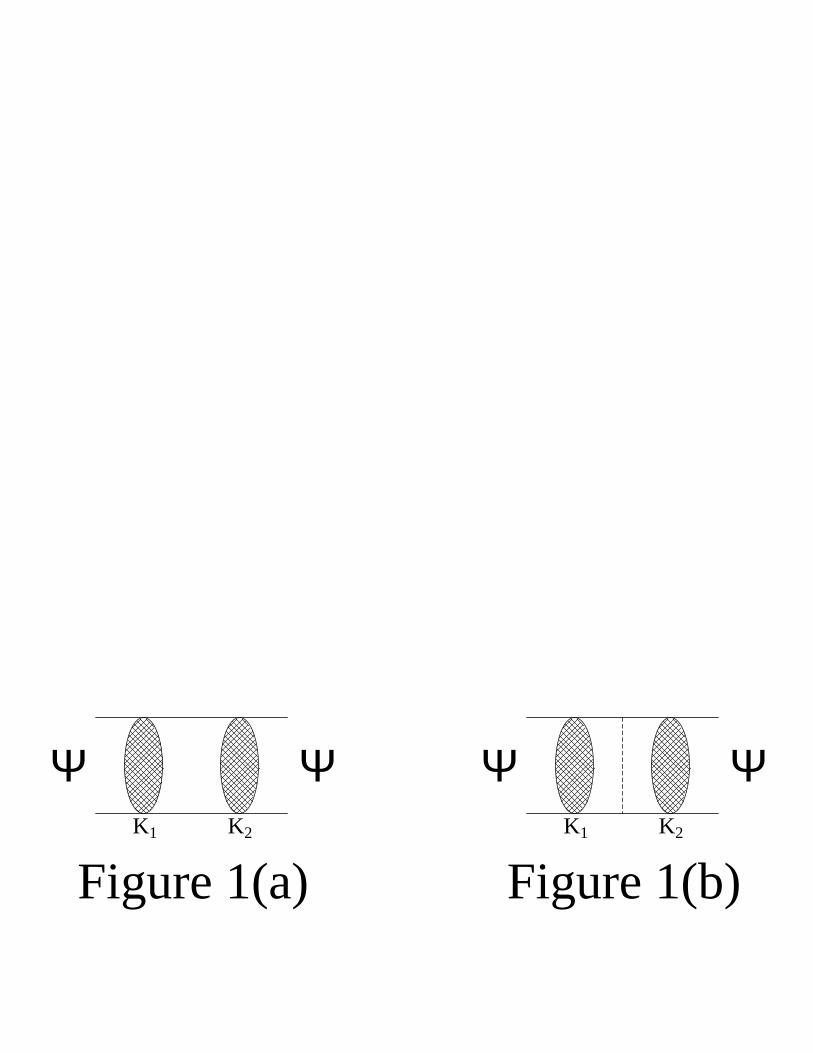
The reason why at least an infinite number of Coulomb kernels must betaken into account in the wavefunction can be easily understood by con-sidering fig.[1a], where a generic bound state diagram is shown. K1 andK2 represent some unspecified kernels. We can schematically represent thisdiagram by

∫

d3k

(2π)3F (k;k) (6)

where F (p1;p2) is a function including the bound state wavefunctions, theinteractions present in the kernels K1 and K2, and the propagator of theelectron-positron pair between these two kernels. The arguments p1 andp2 represent the three-momenta flowing out of the first kernel and into thesecond one. In figure [1a], p1 = p2 = k. As explained above, working withthe effective field theory means that the electron mass no longer appears as adynamical energy scale in the NRQED diagrams; this means that m can onlyappear as an overall factor of the form 1/mn in figure [1a]3. The function F istherefore independent of the electron mass; the only energy scale it depends

3In the language of effective field theories (EFT’s), NRQED is a decoupling EFT withcutoff scale Λ = m. The heavy particle being decoupled is the electron’s antiparticle so

7

on is the typical bound state momentum γ, and the ultraviolet cutoff (whenit is divergent)4.

Let us now consider adding a Coulomb interaction between the two ker-nels, as in fig.[1b]. In conventional scattering theory, one would concludethat this diagram is of higher order than diagram [1a] because of the fac-tor α coming from the vertices. However, this argument does not hold in abound state, because the typical momentum flowing through the Coulombinteraction is of order γ. Indeed, consider how the integral Eq.[6] is modifiedwhen one adds the Coulomb interaction. It must now be written

∫

d3k d3l

(2π)6

ie2

|k − l|2i

(−γ2 − k2)/mF (k; l)

= 4πmα∫ d3k d3l

(2π)6

1

(γ2 + k2)(|k − l|2)F (k; l) (7)

where i/|k − l|2 is the Coulomb propagator and im/(−γ2 − k2) is the non-relativistic propagator for the e−e+ pair.

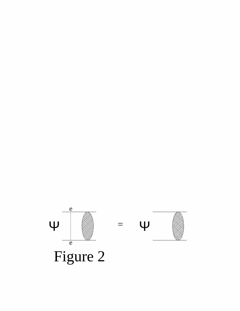
We see that the mass factors out (more about this later!), leaving γ as theonly energy scale in the integral. By dimensional analysis, the final result willbe of order ≃ mα (the overall factor) divided by /γ (from the integral) ≃ 1.This shows that in a bound state, adding a Coulomb interaction does not,in fact, lead to a diagram of higher order. This is why one must sum up allCoulomb interactions in the wavefunctions right from the start. This impliesthe relation expressed in fig.[2] which is nothing else than a diagrammaticrepresentation of the Schrodinger equation.

4.1 Counting rules

The argument we used to show that adding a Coulomb interaction does notincrease the order of a bound state diagram is an example of a NRQED

that Lorentz invariance is broken (as expected in a nonrelativistic theory). Of course,there is a positron in NRQED, but it is here an independent particle; it never appearsas the negative energy pole of the electron propagator (in the language of time-orderedperturbation theory, there are no Z graphs). Consequently, one can apply the decouplingtheorem [5] to NRQED, with the consequence that the heavy scale m will only appear asan overall factor 1/mn in the interactions. One also expects m to enter in the running ofthe low energy coefficients through logarithms, but this dependence on m will only comefrom the QED scattering diagrams, through the matching (see section [5.3].

4We will deal with the infrared divergences separately.

8

counting rule. These rules are extremely important since they permit one toestimate the order of contribution of a diagram without calculating it. Let usfirst consider non-recoil diagrams5. In that approximation, the counting rulesare based on the observation that the mass m of the electron always factorsout of the integrals so that it no longer represents a relevant energy scale.This is clear since m factors out of the nonrelativistic fermion propagators,as we saw in Eq.[7], and it enters the rules of the NRQED vertices only asan overall factor. We therefore see that the use of NRQED eliminates therelativistic energy scale of the system, which, in the light of the discussionin the introduction, greatly simplifies the analysis.

Starting from this observation, we can recast the discussion of the Coulombinteraction in the following manner: adding a Coulomb interaction betweentwo kernels as in fig.[1] leads to an additional factor of α coming from thevertices and a factor of m coming from the additional fermion propagator.The corresponding overall factor of mα must be canceled by a factor havingthe dimensions of energy in order to keep the dimensions straight, but sincethe only energy scale left in the problem is γ, we finally obtain a correctionof order mα/γ ≃ 1. It now becomes obvious that the Coulomb interactionis the only kernel having the property of not increasing the order of a boundstate diagram since all the other interactions contain additional factors of1/m. Each of these 1/m factors will have to be canceled by a correspondingfactor of γ, leading therefore to a result of higher order in α.

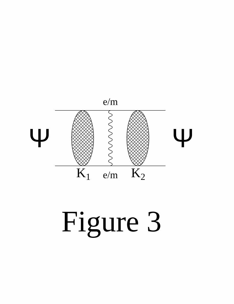
With these rules, it becomes extremely simple to evaluate the order of thecontribution of a given bound state diagram. All we need to know is that theexternal wavefunctions contribute a factor m3α3. To obtain the contributionof a given kernel, one has simply to count the number of explicit factors of α(coming from the vertices) and inverse factors of m (coming from the verticesand the e−e+ propagators) this diagram contains. After canceling the 1/m’swith factors of γ, the number of α’s left over give the order of the contribu-tion of the diagram. Consider, for example, inserting a transverse photon (inthe non-recoil limit) between two wavefunctions as in fig.[3]. The transverse

5In the case of a bound state having equal mass constituents, as positronium, thereis no distinction possible between “recoil effects” and the so-called “retardation effects”.This is not, for example, the case in muonium or hydrogen where (sometimes confusing)distinctions are made between non-recoil and non-retardation approximations. What wemean here by the non-recoil approximation is the limit in which the transverse photondoes not carry any energy.

9

photon vertex has one power of e and one power of 1/m. Taking the twovertices into account, we can conclude that this diagram will contribute toorder m3α3 × α/m2 ≃ mα4 (it is not necessary to multiply by any factor ofγ here). The same is true of the annihilation diagram and of the spin-spininteraction as they also contain a factor of 1/m2 relative to the Coulombinteraction. Another important observation is that these diagrams will con-tribute to only one order6 in α, in contradistinction with Feynman diagramsin conventional Bethe-Salpeter analysis. It is important to understand thatthese rules give the order of contribution of a diagram after the renormal-ization of the effective theory has been performed. Indeed, many NRQEDbound state diagrams are actually badly divergent in the ultraviolet. Therules give us the order of the finite contributions left over after the NRQEDbare coefficients have been renormalized (or, in other words, after matchingwith QED has been performed).

The situation is only slightly more complicated when one takes into ac-count recoil effects. We will not dwell on this issue here, but let us justmention that they make the kinetic energies K enter as a mass scale andthat they are at the origin of the appearance of log’s of α which are charac-teristic of bound states7.

Now that we have a way to estimate the order (in powers of α) of theNRQED diagrams contributions, we can go back to the matching of the ef-fective Lagrangian (Eq.[3]) coefficients with QED. As mentioned earlier, thismatching is done by evaluating scattering amplitudes evaluated in both the-ories. There are two expansions involved in this matching: an expansion innumber of loops in both QED and NRQED, and an expansion in p/m inNRQED. The number of loops n required is found by simply setting mα3+n

equal to the precision desired in the final result (a factor of m3α3 comes fromthe wavefunctions and a factor of 1/m2 comes from the nonrelativistic nor-malization of the Feynman amplitudes). For a given number of loops, thereis an infinite number of nonrelativistic interactions in the effective theory

6We are still limiting ourselves to the non-recoil limit.7To be more precise, the logarithms involve the bound state typical energy scale γ ≃ mα

and the heavy scale Λ = m, leading to a result of the form ln(mα/m) = lnα. This logof m is the one we mentioned earlier when talking about the running of the low energycoefficients. Notice that the infrared cutoff λ always gets canceled while performing thematching because, by construction, the infrared behavior of the effective theory is thesame as the one of the full theory.

10

but, using the counting rules described above, only a finite number must bekept for a given accuracy in the final result. Even if the rules were derivedfor bound state diagrams, they can be directly applied to the NRQED scat-tering diagrams i.e., one imagines sandwiching them between wavefunctionsand one performs the same power counting. Once again there are strongultraviolet divergences but let us repeat that the counting rules give us theorder at which the diagrams will contribute once the matching of the NRQEDcoefficients will have been performed (in other words, once the countertermswill have been included).

There is only one exception to the counting rules, and it occurs whena NRQED scattering diagram contains a power-law infrared divergence. Inthat case, the counting rules must be modified to take into account the pres-ence of a new scale, the infrared cutoff. Take, for example, a scatteringdiagram which has an overall factor of m2α5 times an integral

∫

d3kf(k, γ).The counting rules would suggest that this diagram will contribute by a termof order m2α5/γ = mα4 to the bound state calculation but, if it is linearlyinfrared divergent, it can actually contribute to order m2α5/λ = mα5 (m/λ).Let us mention that this type of diagrams always contain Coulomb interac-tions on external legs and the corresponding integrals are trivial to evaluate.All dependence on the infrared cutoff are due to the sensitivity of theory tolow momenta. Since, in that region, the effective theory is “engineered” toreproduce the full theory (here, QED), these singularities are always presentin the scattering diagrams of both theories so that the renormalized effectivecouplings are always λ independent.

The use of these rules is better explained with the help of a concreteexample. This is what we do in the next section, where we perform anexplicit calculation.

5 Positronium hyperfine splitting

5.1 Order mα4

In this section, we will apply NRQED to a specific calculation, namely thehyperfine splitting8 (E (triplet state) - E (singlet state)) of ground statepositronium. To lowest order, one has the energy levels of the Bohr theory

8Which we will denote by “hfs” in the following.

11

and there is therefore no hfs. To obtain the first non-zero contribution to thesplitting, one has to apply first order perturbation theory to the interactionspresent in the Lagrangian, Eq.[3]. The only interactions that will contributeto the order of interest and that are spin-dependent are

c1e

2mσ · B, (8)

which couples to the transverse photon, and the spin-dependent contact in-teraction involving the electron and positron degrees of freedom (or “annihi-lation” diagram)

d3e2

m2χ†

σψ · ψ†σχ. (9)

All the other interactions, because of the presence of additional powers of1/m, will not contribute to this order.

Now we must fix the coefficients c1 and d3 before computing the hfs.The first coefficient, c1, can be determined by evaluating the spin-flippingscattering of an electron from an external field, in the extreme nonrelativisticlimit. Or one can also simply look up the Pauli Hamiltonian, which the firstfew terms of Eq.[3], at tree level, must reproduce. The end result is thatc1 = 1. The corresponding Feynman rule, in momentum space, is

± e(p′ − p) × σ)

2m(10)

where ± correspond to the electron and the positron, respectively, and p′, p

are the fermion three-momenta after and before the interaction, respectively.The corresponding contribution to the hfs is

−i∫

d3pd3q

(2π)6

(8π1/2γ5/2)2

(p2 + γ2)2(q2 + γ2)2

ψ†[e

2m(q − p) × σ]iψ χ†[−

e

2m(−q + p) × σ]jχ

−i

(p− q)2(δij −

(p − q)i(p− q)j

(p− q)2) (11)

where we have approximated the transverse photon propagator i/(p− q)2 ≃−i/(p − q)2. Physically, this corresponds to neglecting the recoil since onlymomentum, and no energy, is transferred. The corrections to this approxi-mation are of higher order in α.

12

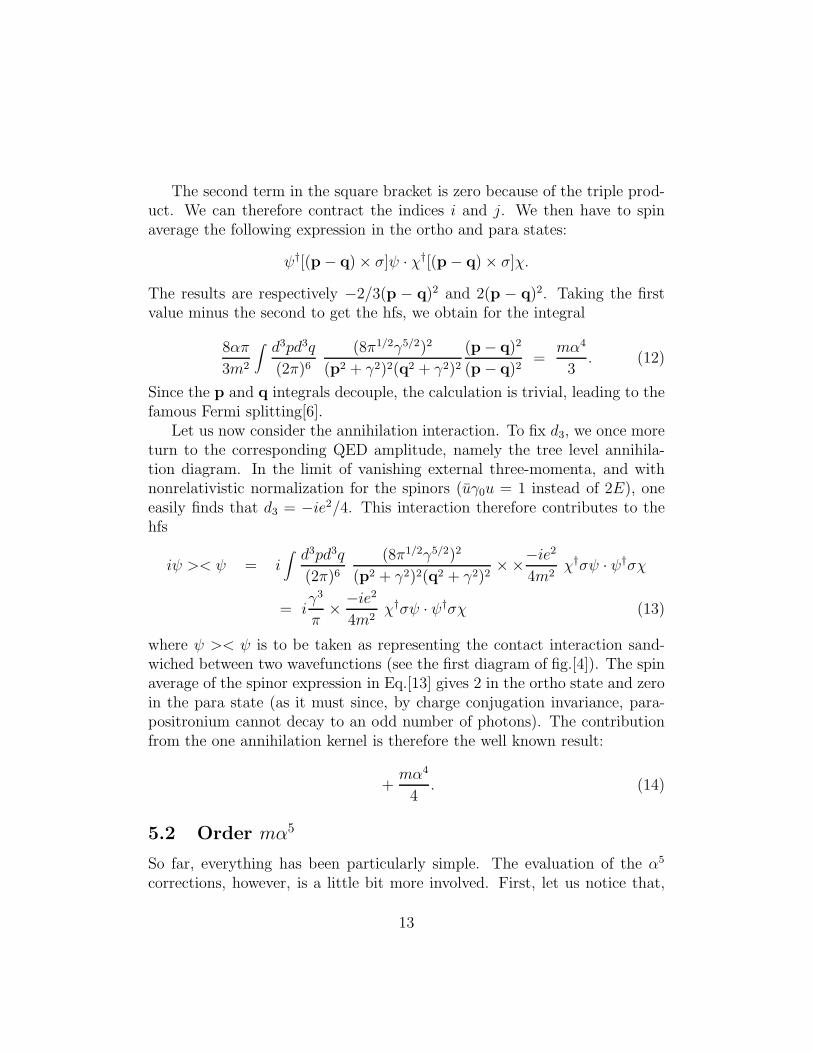
The second term in the square bracket is zero because of the triple prod-uct. We can therefore contract the indices i and j. We then have to spinaverage the following expression in the ortho and para states:

ψ†[(p − q) × σ]ψ · χ†[(p− q) × σ]χ.

The results are respectively −2/3(p − q)2 and 2(p − q)2. Taking the firstvalue minus the second to get the hfs, we obtain for the integral

8απ

3m2

∫

d3pd3q

(2π)6

(8π1/2γ5/2)2

(p2 + γ2)2(q2 + γ2)2

(p − q)2

(p − q)2=

mα4

3. (12)

Since the p and q integrals decouple, the calculation is trivial, leading to thefamous Fermi splitting[6].

Let us now consider the annihilation interaction. To fix d3, we once moreturn to the corresponding QED amplitude, namely the tree level annihila-tion diagram. In the limit of vanishing external three-momenta, and withnonrelativistic normalization for the spinors (uγ0u = 1 instead of 2E), oneeasily finds that d3 = −ie2/4. This interaction therefore contributes to thehfs

iψ >< ψ = i∫

d3pd3q

(2π)6

(8π1/2γ5/2)2

(p2 + γ2)2(q2 + γ2)2××

−ie2

4m2χ†σψ · ψ†σχ

= iγ3

π×

−ie2

4m2χ†σψ · ψ†σχ (13)

where ψ >< ψ is to be taken as representing the contact interaction sand-wiched between two wavefunctions (see the first diagram of fig.[4]). The spinaverage of the spinor expression in Eq.[13] gives 2 in the ortho state and zeroin the para state (as it must since, by charge conjugation invariance, para-positronium cannot decay to an odd number of photons). The contributionfrom the one annihilation kernel is therefore the well known result:

+mα4

4. (14)

5.2 Order mα5

So far, everything has been particularly simple. The evaluation of the α5

corrections, however, is a little bit more involved. First, let us notice that,

13

according to the counting rules given above, it is not possible to identify anydiagram, either in first or second order perturbation theory, that would leadto a contribution of order mα5. As an example, consider the annihilationinteraction in second order perturbation theory (i.e two of these interactionssewn together). The wavefunctions would decouple from the inner loop andlead to a factor of |Ψ(0)|2 = (mα)3/8π. There would be a factor of (e2/m2)2

coming from the two contact interactions, and a factor of m from the nonrel-ativistic propagator. In all we obtain an overall factor of α5 times an integralin which the only energy scale left is µα. The final result will therefore beof order mα6. One can convince oneself that no other diagram can lead to acontribution of order mα5.

Another problem that arises is that, as is well-known from nonrelativisticquantum mechanics, divergences arise when we apply second order pertur-bation theory to the Lagrangian, Eq.[3].

These two difficulties are closely related since they have their origins inthe fact that we have so far entirely neglected relativistic momenta in ouranalysis. This cannot be correct when one goes beyond first order perturba-tion theory since loop momenta are allowed to become arbitrarily high. Asexplained above, the correct way to handle this is to renormalize the “bare”coefficients of NRQED by matching scattering amplitudes in the effectivetheory with QED diagrams.

We will now illustrate this procedure in more details with the contributionfrom the annihilation channel, which is represented by Eq.[13] in NRQED.Renormalizing the coefficient of the contact interaction to one loop meansthat we impose the sum of all one-loop NRQED diagrams involving thisinteraction to be equal to the corresponding one-loop QED diagrams, asshown in fig.[4]. As explained above, the counting rules tell us that there areno NRQED bound state diagrams contributing to order mα6. We know thatthe same must hold true for the NRQED scattering diagrams except if thereare infrared divergent amplitudes. It turns out that there is indeed such anamplitude here, given by the annihilation interaction followed by a Coulombexchange. The corresponding integral is equal to

∫

d3k1

k2

1

k2 + λ2

which can easily be seen to be linearly infrared divergent. It will thereforecontribute to order m2α5/λ and must be included in our calculation.

14

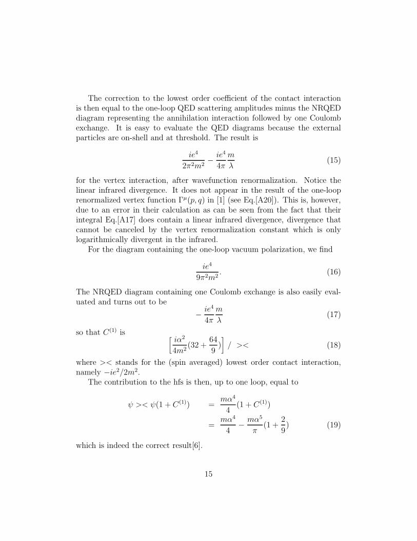
The correction to the lowest order coefficient of the contact interactionis then equal to the one-loop QED scattering amplitudes minus the NRQEDdiagram representing the annihilation interaction followed by one Coulombexchange. It is easy to evaluate the QED diagrams because the externalparticles are on-shell and at threshold. The result is

ie4

2π2m2−ie4

4π

m

λ(15)

for the vertex interaction, after wavefunction renormalization. Notice thelinear infrared divergence. It does not appear in the result of the one-looprenormalized vertex function Γµ(p, q) in [1] (see Eq.[A20]). This is, however,due to an error in their calculation as can be seen from the fact that theirintegral Eq.[A17] does contain a linear infrared divergence, divergence thatcannot be canceled by the vertex renormalization constant which is onlylogarithmically divergent in the infrared.

For the diagram containing the one-loop vacuum polarization, we find

ie4

9π2m2. (16)

The NRQED diagram containing one Coulomb exchange is also easily eval-uated and turns out to be

−ie4

4π

m

λ(17)

so that C(1) is[

iα2

4m2(32 +

64

9)]

/ >< (18)

where >< stands for the (spin averaged) lowest order contact interaction,namely −ie2/2m2.

The contribution to the hfs is then, up to one loop, equal to

ψ >< ψ(1 + C(1)) =mα4

4(1 + C(1))

=mα4

4−mα5

π(1 +

2

9) (19)

which is indeed the correct result[6].

15

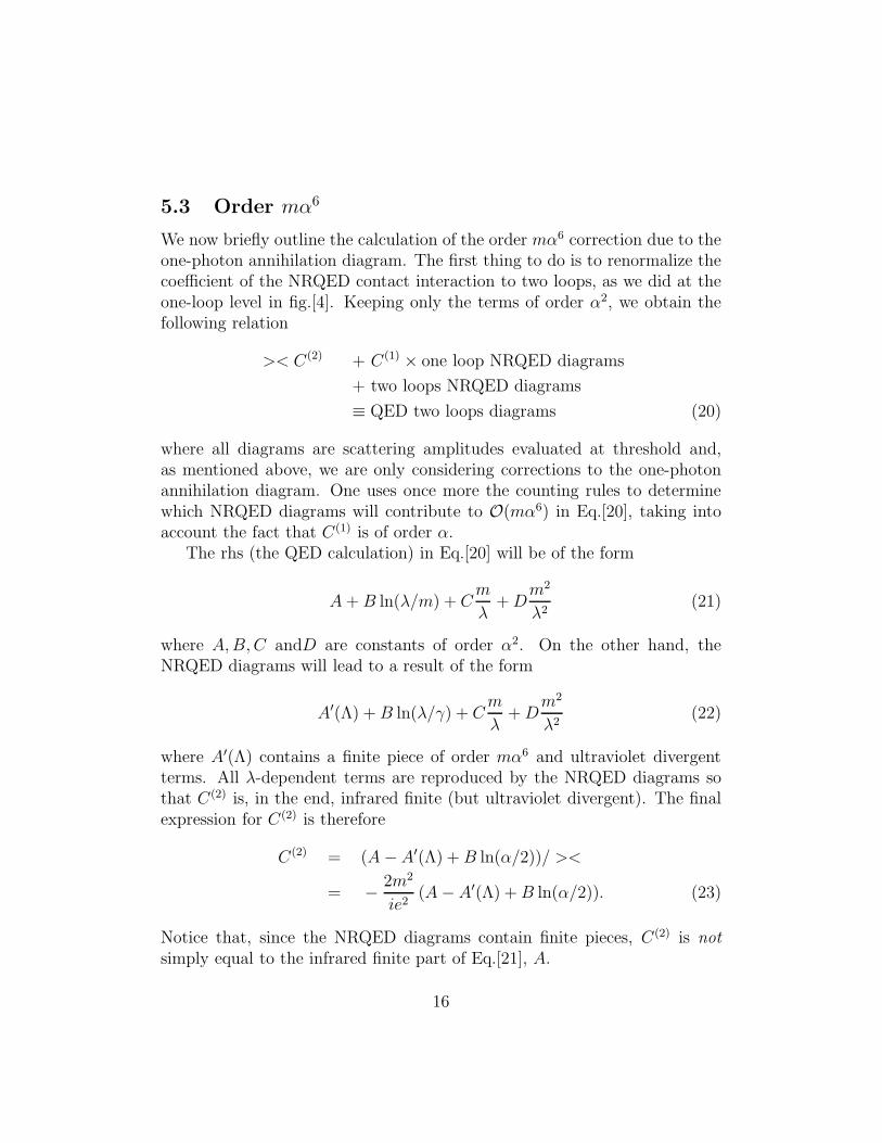
5.3 Order mα6

We now briefly outline the calculation of the order mα6 correction due to theone-photon annihilation diagram. The first thing to do is to renormalize thecoefficient of the NRQED contact interaction to two loops, as we did at theone-loop level in fig.[4]. Keeping only the terms of order α2, we obtain thefollowing relation

>< C(2) + C(1) × one loop NRQED diagrams

+ two loops NRQED diagrams

≡ QED two loops diagrams (20)

where all diagrams are scattering amplitudes evaluated at threshold and,as mentioned above, we are only considering corrections to the one-photonannihilation diagram. One uses once more the counting rules to determinewhich NRQED diagrams will contribute to O(mα6) in Eq.[20], taking intoaccount the fact that C(1) is of order α.

The rhs (the QED calculation) in Eq.[20] will be of the form

A+B ln(λ/m) + Cm

λ+D

m2

λ2(21)

where A,B,C andD are constants of order α2. On the other hand, theNRQED diagrams will lead to a result of the form

A′(Λ) +B ln(λ/γ) + Cm

λ+D

m2

λ2(22)

where A′(Λ) contains a finite piece of order mα6 and ultraviolet divergentterms. All λ-dependent terms are reproduced by the NRQED diagrams sothat C(2) is, in the end, infrared finite (but ultraviolet divergent). The finalexpression for C(2) is therefore

C(2) = (A−A′(Λ) +B ln(α/2))/ ><

= −2m2

ie2(A−A′(Λ) +B ln(α/2)). (23)

Notice that, since the NRQED diagrams contain finite pieces, C(2) is not

simply equal to the infrared finite part of Eq.[21], A.

16

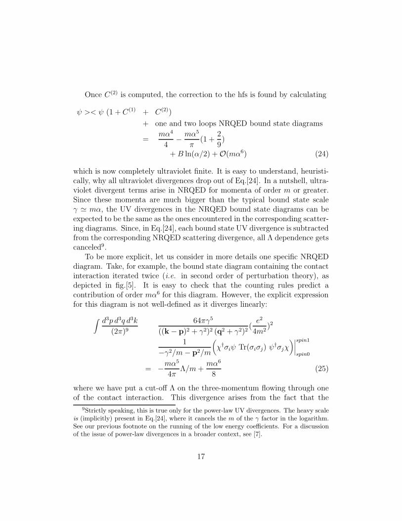
Once C(2) is computed, the correction to the hfs is found by calculating

ψ >< ψ (1 + C(1) + C(2))

+ one and two loops NRQED bound state diagrams

=mα4

4−mα5

π(1 +

2

9)

+B ln(α/2) + O(mα6) (24)

which is now completely ultraviolet finite. It is easy to understand, heuristi-cally, why all ultraviolet divergences drop out of Eq.[24]. In a nutshell, ultra-violet divergent terms arise in NRQED for momenta of order m or greater.Since these momenta are much bigger than the typical bound state scaleγ ≃ mα, the UV divergences in the NRQED bound state diagrams can beexpected to be the same as the ones encountered in the corresponding scatter-ing diagrams. Since, in Eq.[24], each bound state UV divergence is subtractedfrom the corresponding NRQED scattering divergence, all Λ dependence getscanceled9.

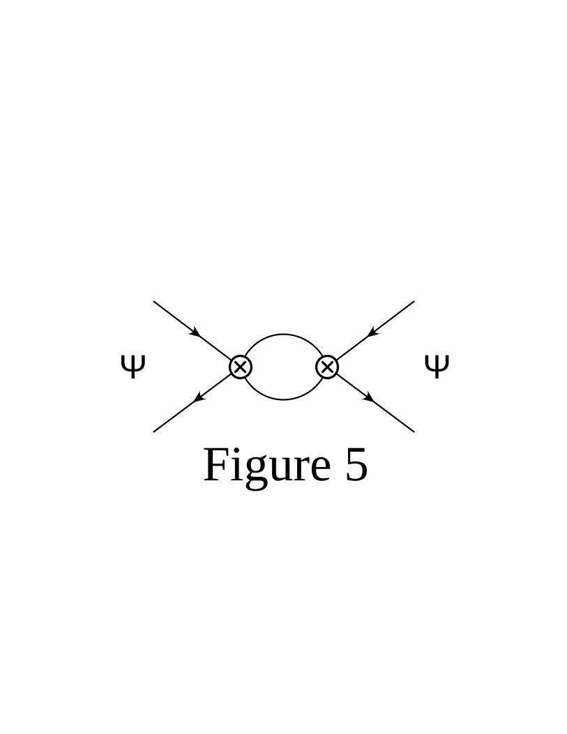
To be more explicit, let us consider in more details one specific NRQEDdiagram. Take, for example, the bound state diagram containing the contactinteraction iterated twice (i.e. in second order of perturbation theory), asdepicted in fig.[5]. It is easy to check that the counting rules predict acontribution of order mα6 for this diagram. However, the explicit expressionfor this diagram is not well-defined as it diverges linearly:

∫ d3p d3q d3k

(2π)9

64πγ5

((k − p)2 + γ2)2 (q2 + γ2)2(e2

4m2)2

1

−γ2/m− p2/m

(

χ†σiψ Tr(σiσj) ψ†σjχ

)∣

∣

∣

∣

spin1

spin0

= −mα5

4πΛ/m+

mα6

8(25)

where we have put a cut-off Λ on the three-momentum flowing through oneof the contact interaction. This divergence arises from the fact that the

9Strictly speaking, this is true only for the power-law UV divergences. The heavy scaleis (implicitly) present in Eq.[24], where it cancels the m of the γ factor in the logarithm.See our previous footnote on the running of the low energy coefficients. For a discussionof the issue of power-law divergences in a broader context, see [7].

17

Lagrangian Eq.[3] is defined for momenta much smaller than the electronmass whereas the momentum in a loop is allowed to become relativistic.However, for p ≥ m, one expects the intermediate state loop to shrink toa point (in coordinate space), as far as the low energy theory is concerned.This means that the divergent contributions to the NRQED bound statediagrams can be canceled by a renormalization of the tree level coefficients.In fact, the necessary counterterms are already present in the coefficientsC(1) and C(2). To see this, let us go back to the definition of C(1), fig.[4].When we calculated the mα5 correction, the only one-loop NRQED diagramwe kept in this equation was the contact interaction followed by a Coulombexchange. Now, however, in order to be consistent in our calculation of ordermα6, we must go back to that equation and include all necessary NRQEDone-loop diagrams. One of those diagrams turns out to be the scatteringdiagram containing the contact interaction iterated twice (i.e fig.[5] with freespinors on the external legs instead of wavefunctions), which has the simpleFeynman rule

−∫ d3k

(2π)3

m

k2(e2

4m2)2 = − 2

α2

m2

Λ

m. (26)

This leads to a new contribution to C(1) and, consequently, to a correctionto bound state energy equal to (see Eq.[24])

− |Ψ(0)|2 ×−2α2

m2

Λ

m=

mα5

4π

Λ

m. (27)

Combining this with Eq.[25] yields a finite correction to the hyperfine split-ting equal to mα6/8.

Before wrapping up this section, we would like to mention that there isyet another new ingredient appearing at order mα6. It has to do with thefact that, as we saw earlier, the Coulomb interaction does not increase theorder (in powers of α) of the bound state diagrams. Although, in first orderperturbation theory this is taken care of by the Schrodinger wavefunctions,in second order one must also sum up the Coulomb interactions in the inter-

mediate state. In practice, this is done by using a closed form expression forthe full Coulomb propagator which has been derived in both coordinate andmomentum space [8].

18

6 Discussion

We have seen that there are two classes of contributions to bound stateproperties, one being characterized by the typical bound state momentump ≈ mα and one characterized by relativistic momenta p ≈ m. Such asituation is ideal for the use of an effective field theory (in the decouplingscenario). NRQED is such a theory, with heavy scale Λ equal to the electronmass m. The use of NRQED greatly simplifies bound state calculations sinceit involves only nonrelativistic interactions in the bound state diagrams andincorporates the relativistic physics via the matching of conventional scat-

tering amplitudes. The relative simplicity of the nonrelativistic interactionsmakes the bound state diagrams easy to evaluate whereas the QED inter-actions appear only in scattering amplitudes, which can be evaluated usingconventional methods. This is to be contrasted with traditional approaches,the Bethe-Salpeter equation for example, which involve the fully relativistictheory in the bound state diagrams, leading to the difficulties discussed inSection 2.

We are finally able to understand in what way the order mα4 and mα5

corrections have a special status: the mα4 corrections come exclusively fromnonrelativistic momenta (i.e. from NRQED diagrams) whereas the mα5

corrections come practically exclusively from relativistic momenta (i.e. fromQED scattering diagrams). We say “practically” because, as we saw in theexample derived above, there is a linear infrared divergence in the QEDdiagrams, showing that they are in fact sensitive to very low momenta. Infact this divergence is a pure threshold singularity, which is due to tha factthat the diagrams are evaluated with external three-momenta set to zero.However, being a low-energy phenomenon, one expects this divergence to bereproduced by NRQED and we saw that this is exactly what happens, inthe form of the Coulomb exchange diagram. But aside from this singularity,which gets canceled when matching QED and NRQED, the mα5 contributionoriginates entirely from QED scattering diagrams10 11.

10Although we have explicitly shown this only for the annihilation diagram, this alsoholds for the p · A interaction; therefore all O(mα5) contributions to the hfs are purelyrelativistic.

11It is in that sense that we call these contributions “purely” relativistic. Maybe amore appropriate terminology would be “bound state independent”. Notice that what wecall “relativistic contributions” are sometimes referred to as “radiative corrections” in the

19

Let us now compare to the technique of Ref.[1]. For the O(mα4) cor-rection, they consider the QED one-photon exchange in the scattering andannihilation channels, expanded them to lowest order in p/m, and obtainedthe expressions Eq.[11] and Eq.[13]. At this order, this is exactly equivalentto using NRQED. In the language of NRQED, these interactions are foundin the effective Lagrangian Eq.[3], which is obtained by taking the nonrel-ativistic limit of the QED Lagrangian. It is in that sense that we call theO(mα4) “purely” nonrelativistic; they are found directly from the effectiveLagrangian.

Now consider the O(mα5) corrections. Once again, we restrict ourselvesto the one-photon annihilation corrections for the sake of simplicity. In ref.[1],these corrections are obtained by sandwiching QED one-loop diagrams be-tween wavefunctions, and taking the limit p → 0 in the QED spinors (thresh-old limit). In that limit, their calculation reduces to multiplying the one-loopthreshold QED diagrams by the square of the wavefunctions evaluated atthe origin. This is almost exactly what we find using NRQED. Indeed the(mα5) term comes uniquely from the renormalization of the NRQED “bare”parameters, as we demonstrated explicitly in this paper. However, there is animportant distinction between the two calculations. In [1], the photon massdependence was discarded, with no further justification. But in NRQED, theλ dependence gets canceled, order by order in the matching procedure. Also,it is now easy to understand why the O(mα5) result for the ground statecan be trivially generalized to ( l = 0) states of arbitrary principal quantumnumber. Indeed, since the only effect of the bound state is to provide anoverall normalization equal to the square of the wavefunction at the origin,the O(mα5) will carry the same dependence on n as |Ψ(0)|2, namely it isproportional to 1/n3.

We are now in position to understand how the two approaches would dif-fer at O(mα6), not only in the handling of the infrared divergences but also inthe prediction of the finite term. We saw in Eq.[24] that, in contradistinctionto the O(mα4) and O(mα5) corrections, the mα6 term contains finite con-tributions from both relativistic and nonrelativistic momenta. Notice thatthis is not simply a consequence of the presence of loops since the O(mα5)term already included integration over internal momenta. It has for origina subtle interplay between relativistic and nonrelativistic flow of momenta

literature.

20

through the Feynman diagrams, interplay which is brought in evidence by theuse of NRQED and its counting rules. Using the rules of [1] would yield therelativistic finite contribution only (in addition to infrared divergent termswhich would have to be discarded without further justification).

The fact that nonrelativistic momenta play an important role at this or-der also has for consequence that it is no longer possible to consider Feynmandiagrams containing only a fixed number of loops, as done in [1]. Indeed, asalready mentioned in Section 5.3, at this order one must consider bound statediagrams with an infinite number of Coulomb interactions in the intermedi-ate states. For example, were we to complete our calculation of the O(mα6)contribution due to the annihilation interaction in second order of perturba-tion theory, we would have to sum up the same diagram with any numberof Coulomb vertices between the two contact interactions. This complica-tion is directly at the origin of the issue of reducible vs irreducible Feynmandiagrams in the Bethe-Salpeter approach. In NRQED, with the help of theCoulomb gauge, this problem is reduced to its most simple form since it isconfined to the Coulomb interaction and the infinite sum can be performedusing the expressions of [8].

Addendum

While writing this paper we became aware of [9], in which one contribution ofO(mα6) is calculated. This contribution corresponds to the one-loop vacuumpolarization correction to the exchange of two photons.

These diagrams, however, lead to purely relativistic corrections or, inother words, they contribute only to the coefficient A in Eq.[23]. This isbecause vacuum polarization is a highly virtual effect (notice that there isno vacuum polarization per se in NRQED; it only enters through the renor-malization of the low energy theory’s coefficients). This can be seen directlyfrom the fact that the corresponding correction to the bound state energy isproportional to the square of the wavefunction at the origin (see Eqs[14-15]in [9]; notice that K is independent of the bound state momenta p and q). Inthat respect, the corrections due to these diagrams are similar to the O(mα5)terms; they are insensitive to bound state physics and can be treated usingthe formalism of [1] (especially since they are infrared finite). An example ofa diagram contributing to O(mα6) that would be sensitive to low momentawould be, for example, the three photon exchange diagrams.

21

Acknowledgments

It is a pleasure to thank G. Peter Lepage for teaching me NRQED and SimonDube for many useful discussions concerning effective field theories. Thiswork has been supported by the Natural Sciences and Engineering ResearchCouncil of Canada.

References

[1] T. Zhang, L. Xiao and R. Koniuk, Can. J. Phys. 70, 670 (1992).

[2] NRQED was introduced in:

W. E. Caswell and G. P. Lepage, Phys. Lett. 167B , 437 (1986).

For pedagogical introductions, see:

“What is renormalization?”, G.P. Lepage, invited lectures given atthe TASI-89 Summer School, Boulder, Colorado; “Quantum Electro-dynamics for Nonrelativistic Systems and High Precision Determina-tions of α”, G.P. Lepage and T. Kinoshita, in Quantum Electrodynam-

ics, T.Kinoshita ed. (World Scientific, Singapore, 1990); “NRQED inbound states: applying renormalization to an effective field theory”, P.Labelle, XIV MRST Proceedings (1992).

[3] E.E. Salpeter and H.A. Bethe, Phys. Rev. 84, 1232 (1951); see alsoreview by S.J. Brodsky, in Atomic Physics and Astrophysics, edited byM. Chretien and E. Lipworth (Gordon and Breach, New York, 1969),Vol. I.

[4] See for example: G.P.Lepage and B.A.Thacker, Nucl.Phys.B (Proc.Suppl.) 4 (1988), 199; B.A. Thacker and G.P.Lepage, Phys. Rev. D

43 (1991), 196; C.T.H. Davies and B.A.Thacker, Ohio State Univer-sity preprint DOE-ER-01545-554, May 1991.; G.P.Lepage et al, CLNSpreprint 92/1136.

[5] T. Appelquist and J. Carazzone, Phys. Rev. D 11, 2856 (1975).

[6] To see the one-photon annihilation mα4 and mα5 contributions to thehfs in positronium, consult

22

Itzykson and Zuber, Quantum Field Theory, McGraw-Hill, 1980, section10.3.

[7] C.P. Burgess and David London, McGill preprint 92/05, hep-ph preprint9203216.

[8] E.H. Wichmann and C.H. Woo, J. Math. Phys. 2, 178 (1961); L. Hostler,J. Math. Phys. 5, 591 (1961); J. Schwinger, J. Math. Phys. 5, 1601(1964).

[9] Tao Zhang and Lixin Xiao, Phys. Rev. A49, 2411 (1994).

23

Ψ ΨK1 K2

Figure 1(a)

Ψ ΨK1 K2

Figure 1(b)

This figure "fig1-1.png" is available in "png" format from:

http://arxiv.org/ps/hep-ph/9407233v1

Ψe

e

Figure 2

= Ψ

This figure "fig1-2.png" is available in "png" format from:

http://arxiv.org/ps/hep-ph/9407233v1

Ψ ΨK1 K2

e/m

e/m

Figure 3

This figure "fig1-3.png" is available in "png" format from:

http://arxiv.org/ps/hep-ph/9407233v1

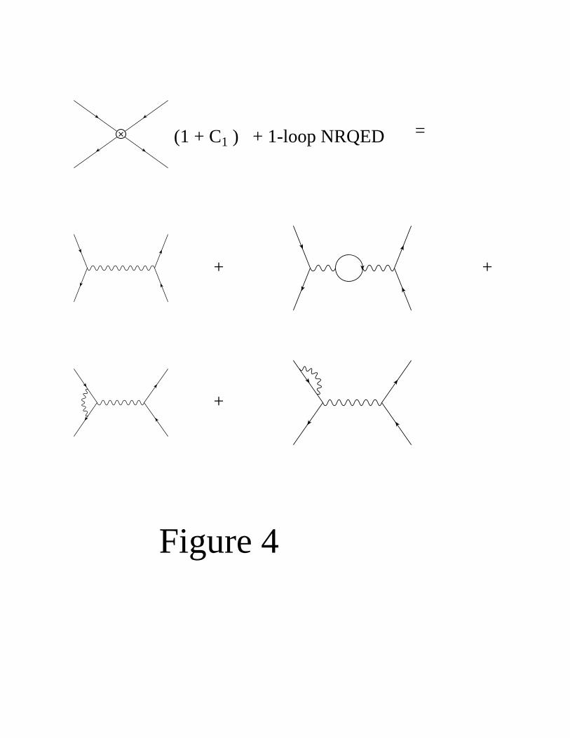
=(1 + C1 ) + 1-loop NRQED

+ +

+

Figure 4

This figure "fig1-4.png" is available in "png" format from:

http://arxiv.org/ps/hep-ph/9407233v1

Ψ Ψ

Figure 5

This figure "fig1-5.png" is available in "png" format from:

http://arxiv.org/ps/hep-ph/9407233v1